Discrete approximation of risk-based prices under volatility uncertainty

Abstract.

We discuss the asymptotic behaviour of risk-based indifference prices of European contingent claims in discrete-time financial markets under volatility uncertainty as the number of intermediate trading periods tends to infinity. The asymptotic risk-based prices form a strongly continuous convex monotone semigroup which is uniquely determined by its infinitesimal generator and therefore only depends on the covariance of the random factors but not on the particular choice of the model. We further compare the risk-based prices with the worst-case prices given by the $G$-expectation and investigate their asymptotic behaviour as the risk aversion of the agent tends to infinity. The theoretical results are illustrated with several examples and numerical simulations showing, in particular, that the risk-based prices lead to a significant reduction of the bid-ask spread compared to the worst-case prices.

Key words: risk-based pricing, indifference pricing, volatility uncertainty, nonlinear semigroup, Chernoff approximation.

MSC 2020 Classification: Primary 91G20, 47H20; Secondary 91G70, 91G60, 47J25.

1. Introduction

Computing the prices of financial derivatives strongly depends on the choice of the underlying model and the associated probability distributions. Since these distributions are, in general, not precisely known, robust finance takes into account model uncertainty by considering sets of possible transition probabilities. In this article, we start with a simple asset model in discrete time for which derivative prices can easily be computed by backward recursion and analyze the asymptotic behaviour of derivative prices as the number of intermediate trading periods tends to infinity. A classical example of this is the convergence of derivative prices in the binomial model to the Bachelier or Black–Scholes prices, see e.g. [43, Section 5.7]. Discrete financial models are generally straightforward from a modeling perspective and arise naturally since trading typically occurs at discrete time points. Nonetheless, continuous-time models are very popular since they allow for the use of stochastic calculus and PDE methods. Furthermore, it has recently been shown in [32] that superhedging prices of discrete-time models with uncertain Markovian transition kernels converge to superhedging prices of continuous-time models with drift and volatility uncertainty. Superhedging prices correspond to intervals of plausible prices which do not generate arbitrage opportunities, see for example [34]. Although such intervals can naturally be associated with an arbitrage-free bid-ask spread, these bounds are, in general, too wide to be informative about the prices of a contingent claim in incomplete markets. In fact, each agent operating in the market assigns a different subjective value to the same contingent claim which can violate the bounds prescribed by the superhedging or subhedging prices.

A classical approach to reduce the bid-ask spread observable in incomplete markets consists of taking the preferences of an agent into account by associating a utility function or a risk measure to the agent. A strand of literature has developed in this direction introducing so-called good deals bounds. Good deals bounds aim to reduce the no-arbitrage bounds by ruling out prices that can be hedged by strategies leading to a high expected utility, i.e., prices that represent a deal which is too good. Good deals have been measured by means of Sharpe ratios [31], gain-loss ratios [12] or utility functions [27, 15, 28]. Moreover, the setting in [42] allows for imperfect hedges as long as their level of risk is acceptable. Closely related to good deal prices are indifference prices which make the agent indifferent regarding her utility or risk between selling or keeping the derivative, see [82, 76, 55, 13, 14]. A connection between the two concepts was first established in [54], where it is shown that indifference prices based on coherent risk measures are equivalent to the good deal prices in [28]. Furthermore, every convex risk measure representing good deal prices is given by an indifference price, see [2]. An extensive collection of the literature on good deal and indifference prices can be found in [26]. So far, explicit solutions have only been given in dominated settings, where the asset process is given with respect to a physical measure $\mathbb{P}$ and the absence of good deals translates into restrictions on the set of equivalent local martingale measures $\{\mathbb{Q}\}_{\mathbb{Q}\sim\mathbb{P}}$. However, since incompleteness in a market is naturally connected with model uncertainty and the inability to precisely estimate the distribution of the assets, a more general framework taking model uncertainty into account seems to be necessary. In addition, as pointed out in [79], classical indifference pricing often has the flavour of a one-period model.

In this article, we work in a non-dominated setting, where the uncertain distribution of the increments of the asset process is determined by a sublinear expectation $\mathcal{E}[\,\cdot\,]$. Moreover, we consider an agent who measures the risk associated to a random loss $Y$ by means of a robust entropic risk measure

$$\rho[Y]:=\frac{1}{\alpha}\log\big{(}\mathcal{E}\big{[}e^{\alpha Y}\big{]}\big{)},$$

where $\alpha>0$ is a risk aversion parameter. Since the entropic risk measure is the certainty equivalent of the exponential utility, our agent can also be seen as a robust exponential utility maximizer whose preferences belong to the class of multiple priors preferences which have been introduced and characterized in [46]. The term robust refers to the consideration of several plausible models which can be derived from the dual representation

$$\mathcal{E}[Y]=\sup_{\mathbb{Q}\in\mathcal{Q}}\mathbb{E}_{\mathbb{Q}}[Y]$$

of the sublinear expectation. For a brief introduction to sublinear expectations, we refer to Subsection 2.1 and the references therein. Following the previously mentioned work [46] and its extension [59], the problem of robust pricing has gained a great deal of attention. In particular, we refer to [10, 38, 23, 1, 11, 24] for arbitrage theory and superhedging dualities under model uncertainty and to [39, 30, 40] for similar results in the presence of transaction costs and trading constraints. The multiple priors problem has also been tackled in the context of utility maximization in dominated settings, see [73, 48, 67, 5] and in non-dominated settings, see [36, 66, 64, 65]. In the specific context of exponential utility, the authors of [44, 33] prove duality in a continuous-time non-robust setting. Furthermore, in [75, 51] the value function of the utility maximization problem is characterized via a quadratic BSDE and several properties of the pricing functional such as monotonicity and the asymptotic behaviour w.r.t. the risk aversion parameter are derived. These results have been extended in [60] and, for a non-dominated setting, in [61]. For unbounded claims, duality and the existence of maximizers have been established in [6] and, under the presence of transaction costs, in [35].

Starting from a $d$-dimensional discrete-time market, we assume that the asset process $X$ has independent increments which are determined by the equation

$$X_{(k+1)h}-X_{kh}=h\mu+\sqrt{h}\zeta\quad\mbox{for all }k\in\mathbb{N},$$

where $h>0$ is a fixed step-size, $\mu\in{\mathbb{R}^{d}}$ is a deterministic drift and $\zeta$ is a $d$-dimensional random vector with mean zero. Given a claim with payoff function $f$ and maturity $T=Nh$, the indifference ask price $a_{T}(f)\in\mathbb{R}$ is uniquely determined by the relation

$$\inf_{\theta=(\theta_{1},\dots,\theta_{N})}\rho\big{[}f(X_{T})-a_{T}(f)-(\theta\cdot X)_{T}\big{]}=\inf_{\theta=(\theta_{1},\dots,\theta_{N})}\rho[-(\theta\cdot X)_{T}],$$

where the random variables $\theta_{1},\dots,\theta_{N}\colon\Omega\to\Theta$ take values in a set of available strategies $\Theta\subset{\mathbb{R}^{d}}$ such that $\theta_{k}$ is $X_{(k-1)h}$-measurable for all $k=1,\ldots,N$ and

$$(\theta\cdot X)_{T}:=\sum_{k=1}^{N}\theta_{k}(X_{kh}-X_{(k-1)h}).$$

Under suitable conditions, one can show that $a_{T}\colon{\rm C}_{\rm b}\to{\rm C}_{\rm b}$, where ${\rm C}_{\rm b}$ consists of all bounded continuous functions $f\colon{\mathbb{R}^{d}}\to\mathbb{R}$. Hence, if we require the indifference ask prices to be time consistent, they are completely determined by the one-step pricing operator $I(h)f:=a_{h}(f)$ and the equation

$$a_{T}(f)=I(h)^{N}f\quad\mbox{for all }T=Nh\mbox{ and }f\in{\rm C}_{\rm b}.$$ (1.1)

Dynamic consistency has previously been imposed in [31] to solve the multi-period pricing problem by iterating the solution of the one-period model. Furthermore, in a continuous-time setting, the authors of [56] show that local conditions on the pricing kernels guarantee nice global properties of the pricing operator, included time-consistency. In Subsection 2.3, dynamically consistent pricing operators are discussed in more detail. We are now interested in the limit behaviour of the multi-step prices as the number of intermediate trading periods tends to infinity. For that purpose, let $t\geq 0$ be a maturity and $h_{n}:=t/n$ be a sequence of decreasing step-sizes. Then, if the limit

$$a_{t}^{\infty}(f):=\lim_{n\to\infty}a_{t}^{(n)}(f)$$ (1.2)

of the multi-step indifference prices exists, it defines the asymptotic risk-based price of a claim with payoff function $f$ and maturity $t$. In order to prove that the previous limit exists and to uniquely characterize the global dynamics of the asymptotic risk-based prices by means of their infinitesimal bevahiour, we reformulate equation (1.2) as an approximation result of a nonlinear semigroup. This view point is motivated by the fact that the time consistency of the multi-period prices transfers to the limit, i.e.,

$$a_{s+t}^{\infty}(f)=a_{s}^{\infty}(a_{t}^{\infty}(f))\quad\mbox{for all }s,t\geq 0.$$ (1.3)

Equation (1.1) guarantees that the right-hand side of equation (1.2) is given by

$$a_{t}^{(n)}(f)=I\big{(}\tfrac{t}{n}\big{)}^{n}f\quad\mbox{for all }t\geq 0,f\in{\rm C}_{\rm b}\mbox{ and }n\in\mathbb{N},$$

where $I(h)\colon{\rm C}_{\rm b}\to{\rm C}_{\rm b}$ denotes the pricing operator for one period with step size $h\geq 0$. Furthermore, these operators have desirable properties such as convexity and monotonicity. The question whether a sequence of iterated operators $(I(\tfrac{t}{n})^{n})_{n\in\mathbb{N}}$ on ${\rm C}_{\rm b}$ converges to a limit operator $S(t)\colon{\rm C}_{\rm b}\to{\rm C}_{\rm b}$ such that $(S(t))_{t\geq 0}$ is a strongly continuous convex monotone semigroup has systematically been addressed in a series of recent articles, see [18, 21, 20, 22]. Applying these results to the present setting shows that the limit

$$S(t)f:=\lim_{n\to\infty}I\big{(}\tfrac{t}{n}\big{)}^{n}f$$

exists for all $t\geq 0$ and $f\in{\rm C}_{\rm b}$. Moreover, the family $(S(t))_{t\geq 0}$ is a strongly continuous convex monotone semigroup which is uniquely determined by its infinitesimal generator

$$Af:=\lim_{h\downarrow 0}\frac{S(h)f-f}{h}.$$

The asymptotic risk-based prices are then defined by

$$a_{t}^{\infty}(f):=S(t)f\quad\mbox{for all }t\geq 0\mbox{ and }f\in{\rm C}_{\rm b}.$$

Note that, by equation (1.2) and (1.3), these prices are time consistent and given as the limit of multi-period prices in a discrete model. In addition, the prices have desirable properties such as convexity and monotonicity w.r.t. the payoff function. So far, we did not address the question whether the asymptotic risk-based prices depend on the particular choice of the discrete model. In case of the previously mentioned approximation of the Bachelier prices, the central limit theorem guarantees that the Bachelier prices only depend on the covariance of the discrete model but not on the particular choice of its distribution. This observation is a particular case of the more general statement that strongly continuous semigroups are uniquely determined by their generators. For linear semigroups the uniqueness is classical result and for convex monotone semigroups it has been proven in [18, 20]. In the present article, the generator can explicitly be computed as

$$Af=\inf_{\theta\in\Theta}\Big{(}G\big{(}D^{2}f+\alpha(Df-\theta)(Df-\theta)^{T}\big{)}+(Df-\theta)^{T}\mu\Big{)}-\inf_{\theta\in\Theta}\Big{(}G\big{(}\alpha\theta\theta^{T}\big{)}-\theta^{T}\mu\Big{)},$$

for sufficiently smooth functions $f$, where $\Theta\subset{\mathbb{R}^{d}}$ is a set of available trading strategies and the function

$$G\colon\mathbb{R}^{d\times d}\to\mathbb{R},\;a\mapsto\frac{1}{2}\mathcal{E}\big{[}\zeta^{T}a\zeta\big{]}$$

describes the covariance of the random factors. In particular, the asymptotic risk-based prices only depend on the covariance of the discrete model but not on the particular choice of its distribution. In Subsection 2.2, we explain the semigroup approach in more detail and fix the precise terminology used throughout the rest of this article. Furthermore, at the beginning of Section 5, we recall the precise statements from [18] on which the proofs of the main results in this article are based.

In the following, the main results of this article are described in more detail. In order to guarantee the well-posedness of the one-step pricing operators and to exlcude doubling strategies as the number of intermediate trading periods tends to infinity, we first impose a volume constraint on the set of available trading strategies, see Theorem 3.2. Since the asymptotic risk-based prices are uniquely determined by the covariance of the random factors, a non-degeneracy condition guarantees that the volume constraint can be arbitrarily large, see Theorem 3.3. This way, we can define asymptotic risk-based prices involving unbounded sets of trading strategies as limits of volume constrained prices. Modeling the set $\Theta$ allows to impose constraints on the available trading strategies such as volume or short-selling constraints, non-tradable assets, etc. However, in the absence of trading constraints, the generator does not depended on the gradient and is given by

$$Af=\inf_{\theta\in{\mathbb{R}^{d}}}\Big{(}G\big{(}D^{2}f+\alpha\theta\theta^{T}\big{)}-\theta^{T}\mu\Big{)}-\inf_{\theta\in{\mathbb{R}^{d}}}\Big{(}G\big{(}\alpha\theta\theta^{T}\big{)}-\theta^{T}\mu\Big{)}.$$

In particular, the risk-based prices taking into account the attitude of the agent towards risk are always dominated by the worst-case prices associated to the $G$-expectation, see Corollary 3.4. So far, in the absence of trading constraints, we did not define the asymptotic risk-based prices as the limit of multi-step prices, but as the limit of volume constrained asymptotic prices. However, under additional conditions on the distribution, the asymptotic prices can be obtained as the limit of the unconstrained multi-step prices, see Theorem 3.5. Finally, we are interested in the asymptotic behaviour of the prices as the risk aversion of the agent tends to infinity. For a dominated continuous-time framework, it has been shown in [75, 60] that the value of the utility maximization problem converges to the superhedging price as the risk aversion tends to infinity. In a non-dominated discrete-time setting, the same result has later been obtained in [6, 35], see also [25, 16] for similar results. Moreover, for finite state spaces and for downside-sensitive preferences, it has been shown in [28] that the risk-based price bounds approach the no-arbitrage ones as the set of desirable claims gets smaller. In this article, we impose a uniform ellipticity condition on the covariance of the random factors to show that the asymptotic risk-based prices converge to the worst-case prices associated to the $G$-expectation as the risk aversion tends to infinity, see Theorem 3.6.

Apart from the novel theoretical insights regarding the converge of the multi-step prices to the asymptotic risk-based prices, Chernoff-type approximations also provide a tool for numerical approximations which is illustrated in Section 4. For instance, since the asymptotic risk-based prices only depend on the covariance structure of the model but not on the particular choice of the distribution, it is sufficient to recursively compute the indifference prices in the binomial model for every trading period. This also works well in the presence of model uncertainty, see Subsection 4.2 and Subsection 4.4. Furthermore, the numerical simulations in Subsection 4.3 confirm that the asymptotic prices only depends on the covariance of the increments although the precise bounds for the difference between the multi-step prices and the asymptotic prices might depend on the choice of the model. Convergence rates for Chernoff-type approximations have been investigated in [19] but addressing this question in the present context is beyond the scope of this article. So far, we focused on ask prices derived from the view point of the seller. Similarly, from the perspective of the buyer, one can derive the corresponding bid prices $b_{t}^{\infty}(f)$ which are related to the ask prices via the equation $b_{t}^{\infty}(f)=-a_{t}^{\infty}(-f)$. In particular, the bid-ask spread for the risk-based prices is always smaller than the the bid-ask spread for the worst-case prices associated to the $G$-expectation, see Subsection 4.5.

The rest of this article is organized as follows: in Section 2, we introduce the market model, the asset distribution given by a sublinear expectation, dynamically consistent pricing operators and the necessary terminology regarding strongly continuous convex monotone semigroups. Section 3 first introduces the agent’s preferences and indifference pricing relations before stating the main results. Section 4 contains several examples in order to illustrate the abstract results including numerical simulations. The proofs of the main results are given in Section 5. Finally, Appendix A contains a basic convexity estimates and elementary properties of sublinear expectations while Appendix B contains some exponential moment estimates.

2. Market model and pricing operators

We consider $d\in\mathbb{N}$ financial assets $X=(X^{1},\dots,X^{d})^{T}$ which are traded at discounted prices $X_{kh}$ at discrete time-points $\mathcal{T}(h):=\{kh\colon k\in\mathbb{N}_{0}\}$ for some trading period $h>0$. All prices/payoffs are discounted by expressing them in terms of a numéraire $S^{0}$ which is strictly positive in all possible states at all considered trading times, i.e., the discounted value of a random payoff $Z$ at time $t\in\mathcal{T}(h)$ is given by $Z/S^{0}_{t}$. Furthermore, the asset prices start at $X_{0}^{x}:=x\in\mathbb{R}^{d}$ and follow the dynamics

$$X_{(k+1)h}^{x}:=X_{kh}^{x}+h\mu+\sqrt{h}\zeta_{k+1}\quad\mbox{for all }k\in\mathbb{N},$$ (2.1)

where $\mu\in\mathbb{R}^{d}$ is a deterministic drift and $(\zeta_{k})_{k\in\mathbb{N}}$ are i.i.d. random vectors $\zeta_{k}\colon\Omega\to\mathbb{R}^{d}$ on a sublinear expectation space $(\Omega,\mathcal{H},\mathcal{E})$ which will be specified in the following subsection.

2.1. Asset distribution and sublinear expectations

A sublinear expectation space $(\Omega,\mathcal{H},\mathcal{E})$ consists of a set $\Omega$, a pointwise ordered linear space $\mathcal{H}$ of random variables $Y\colon\Omega\to\mathbb{R}$ with $c\mathds{1}_{\Omega}\in\mathcal{H}$ and $|Y|\in\mathcal{H}$ for all $c\in\mathbb{R}$ and $Y\in\mathcal{H}$ and a sublinear expectation $\mathcal{E}\colon\mathcal{H}\to\mathbb{R}$ satisfying

1. $\mathcal{E}[c\mathds{1}_{\Omega}]=c$ for all $c\in\mathbb{R}$,

2. $\mathcal{E}[Y]\leq\mathcal{E}[Z]$ for all $Y,Z\in\mathcal{H}$ with $Y\leq Z$,

3. $\mathcal{E}[Y+Z]\leq\mathcal{E}[Y]+\mathcal{E}[Z]$ for all $Y,Z\in\mathcal{H}$,

4. $\mathcal{E}[\lambda Y]=\lambda\mathcal{E}[Y]$ for all $Y\in\mathcal{H}$ and $\lambda\geq 0$.

The sublinear expectation is called continuous from above if $\mathcal{E}[X_{n}]\downarrow 0$ for all sequences $(X_{n})_{n\in\mathbb{N}}$ with $X_{n}\downarrow 0$. Note that the properties (i) an (iii) imply cash invariance, i.e., it holds $\mathcal{E}[Y+c]=\mathcal{E}[Y]+c$ for all $Y\in\mathcal{H}$ and $c\in\mathbb{R}$. Sublinear expectations were introduced by Peng to incorporate model uncertainty of the asset distribution, see [71] for a detailed discussion. Indeed, the formula

$$\mathcal{E}[Y]:=\sup_{\mathbb{Q}\in\mathcal{Q}}\mathbb{E}_{\mathbb{Q}}[Y]\quad\text{for all }Y\in\mathcal{H}$$ (2.2)

defines a sublinear expectation, where the supremum is taken over an uncertainty set $\mathcal{Q}$ of probability measures on $(\Omega,\sigma(\mathcal{H}))$. On the other hand, every sublinear expectation which is continuous from above admits such a representation, see [71, Theorem 1.2.2]. Sublinear expectations are also closely related to several other concepts such as coherent risk measures in mathematical finance [3], upper expectations in robust statistics [53] and upper coherent previsions in the theory of imprecise probabilities [80]. In a dynamic setting sublinear expectations are linked to BSDEs [41, 74, 77]. Instead of specifying the space $\mathcal{H}$, we rather assume that it is rich enough to guarantee that $(\zeta_{k})_{k\in\mathbb{N}}\subset\mathcal{H}^{d}$ and that all the terms appearing in the following are again elements of $\mathcal{H}$. In particular, we assume that $f(\zeta_{1},\ldots,\zeta_{n})\in\mathcal{H}$ for all $n\in\mathbb{N}$ and $f\in{\rm Lip}_{\rm b}((\mathbb{R}^{d})^{n})$, where ${\rm Lip}_{\rm b}((\mathbb{R}^{d})^{n})$ denotes the space of all bounded Lipschitz-continuous functions $f\colon(\mathbb{R}^{d})^{n}\to\mathbb{R}$. The random vectors $(\zeta_{k})_{k\in\mathbb{N}}$ are supposed to be independent and identically distributed (i.i.d.) meaning that

$$\mathcal{E}[f(\zeta_{m})]=\mathcal{E}[f(\zeta_{n})]\quad\mbox{for all }f\in{\rm Lip}_{\rm b}(\mathbb{R}^{d})\mbox{ and }m,n\in\mathbb{N}$$

and that $\zeta_{n+1}$ is independent of $\zeta_{1},\dots,\zeta_{n}$ for all $n\in\mathbb{N}$, i.e.,

$$\mathcal{E}\left[f(\zeta_{1},\dots,\zeta_{n},\zeta_{n+1})\right]=\mathcal{E}\left[\mathcal{E}[f(z,\zeta_{n+1})]\big{|}_{z=(\zeta_{1},\dots,\zeta_{n})}\right]\quad\mbox{for all }f\in{\rm Lip}_{\rm b}((\mathbb{R}^{d})^{n}\times\mathbb{R}^{d}).$$

Furthermore, the random vectors have no mean uncertainty, i.e.,

$$\mathcal{E}[a^{T}\zeta_{1}]=0\quad\mbox{for all }a\in\mathbb{R}^{d}.$$ (2.3)

For the sake of illustration, we provide several examples for the uncertain asset distribution given by the functional ${\rm C}_{\rm b}\to\mathbb{R},\;f\mapsto\mathcal{E}[f(\zeta_{1})]$, where the space ${\rm C}_{\rm b}:={\rm C}_{\rm b}({\mathbb{R}^{d}})$ consists of all bounded continuous functions $f\colon{\mathbb{R}^{d}}\to\mathbb{R}$. Since we have already assumed that $f(\zeta_{1})\in\mathcal{H}$ for all $f\in{\rm Lip}_{\rm b}:={\rm Lip}_{\rm b}({\mathbb{R}^{d}})$, the term $\mathcal{E}[f(\zeta_{1})]$ is also well-defined for all $f\in{\rm C}_{\rm b}$ if the sublinear expectation $\mathcal{E}$ is continuous from above. The latter is valid if the supremum in equation (2.2) is taken over a tight set of probability measures.

Example 2.1.

1. Without uncertainty, the measure $\nu:=\mathbb{P}\circ\zeta_{1}^{-1}$ determines the linear expectation

   $$\mathcal{E}[f(\zeta_{1})]:=\mathbb{E}_{\mathbb{P}}[f(\zeta_{1})]=\int_{{\mathbb{R}^{d}}}f\,{\rm d}\nu\quad\text{for all }f\in{\rm C}_{\rm b}$$

   and condition (2.3) reduces to $\int_{\mathbb{R}^{d}}x\,\nu({\rm d}x)=0$.

2. Let $\nu$ be a probability measure on $({\mathbb{R}^{d}},\mathcal{B}({\mathbb{R}^{d}}))$ and $\Lambda\subset{\mathbb{R}^{d}}$ be a bounded set. Perturbing the values of $\zeta_{1}$ by $\pm\lambda$ leads to a sublinear distribution incorporating parametric uncertainty given by

   $$\mathcal{E}[f(\zeta_{1})]:=\sup_{\lambda\in\Lambda}\frac{1}{2}\int_{{\mathbb{R}^{d}}}f(x+\lambda)+f(x-\lambda)\,\nu({\rm d}x)\quad\text{for all }f\in{\rm C}_{\rm b}.$$

   Condition (2.3) is satisfied if $\int_{\mathbb{R}^{d}}x\,\nu({\rm d}x)=0$ and for $\Lambda=\{0\}$ we recover the linear case without uncertainty. As a particular one-dimensional example of this parametrization, we choose the Dirac measure $\nu:=\delta_{0}$ and $\Lambda:=[\sigma_{0}-u,\sigma_{0}+u]$, where $\sigma_{0}>0$ is a reference volatility and $u\in[0,\sigma_{0}]$ is the level of uncertainty. Then, the sublinear expectation

   $$\mathcal{E}[f(\zeta_{1})]:=\sup_{\sigma\in[\sigma_{0}-u,\sigma_{0}+u]}\frac{1}{2}\big{(}f(\sigma)+f(-\sigma)\big{)}\quad\text{for all }f\in{\rm C}_{\rm b}$$

   describes a binomial model with uncertain volatility. We also want to mention that, for every $\lambda\in\Lambda$, the distribution $\nu$ is transformed to the distribution

   $$\nu\kappa_{\lambda}(B):=\int_{\mathbb{R}^{d}}\kappa_{\lambda}(x,B)\,\nu({\rm d}x)\quad\text{for all }B\in\mathcal{B}({\mathbb{R}^{d}})$$

   through the weak transport plan $\kappa_{\lambda}(x,B):=\frac{1}{2}\delta_{x+\lambda}(B)+\frac{1}{2}\delta_{x-\lambda}(B)$. For uncertainty sets based on weak optimal transport, we refer to [58] and the references therein.

3. In recent years, non-parametric uncertainty has been becoming increasingly popular and has been explored extensively, for instance, in the field of distributionally robust optimization, see, e.g, [8, 17, 45, 62, 72, 81, 83]. The analytical tractability of transport distances such as the Wasserstein distance allows for dual representations and explicit sensitivity analysis, see [7, 9]. Let $\nu$ be a reference distribution with $\int_{\mathbb{R}^{d}}x\,\nu({\rm d}x)=0$ and $\int_{\mathbb{R}^{d}}|x|^{p}\,\nu({\rm d}x)<\infty$ for some $p>2$. We define

   $$\mathcal{E}[f(\zeta_{1})]:=\sup_{\mathcal{W}_{0}(\nu,\tilde{\nu})\leq u}\int_{{\mathbb{R}^{d}}}f\,{\rm d}\tilde{\nu}\quad\text{for all }f\in{\rm C}_{\rm b},$$

   where $u\geq 0$ is the level of uncertainty and the transport distance $\mathcal{W}_{0}$ is given by

   $$\mathcal{W}_{0}(\nu,\tilde{\nu}):=\left(\inf_{\pi\in\Pi_{0}(\nu,\tilde{\nu})}\int_{\mathbb{R}^{d}\times\mathbb{R}^{d}}|x-y|^{p}\,\pi({\rm d}x,{\rm d}y)\right)^{\frac{1}{p}}$$

   with the infimum being taken over the set $\Pi_{0}(\nu,\tilde{\nu})$ of all couplings between $\nu$ and $\tilde{\nu}$ satisfying $\int_{\mathbb{R}^{d}\times\mathbb{R}^{d}}x^{T}a(y-x)\,\pi({\rm d}x,{\rm d}y)=0$ for all symmetric $d\times d$-matrices $a$. Alternatively, the set $\Pi_{0}(\nu,\tilde{\nu})$ can be replaced by the set of all martingale couplings. For details, we refer to [21, Section 4.2].

2.2. Continuous time limits and Chernoff-type approximations

So far, we considered asset prices following the dynamics given by equation (2.1) in a discrete-time framework with fixed step-size $h>0$. Now, we are interested in the limit behaviour of the asset dynamics as the number of intermediate trading periods tends to infinity. Let $t\geq 0$, $x\in{\mathbb{R}^{d}}$ and $h_{n}:=t/n$ for all $n\in\mathbb{N}$. We define $X_{0}^{n,x}:=x$ and

$$X_{(k+1)h_{n}}^{n,x}:=X_{kh}^{n,x}+h_{n}\mu+\sqrt{h_{n}}\zeta_{k+1}\quad\mbox{for all }k,n\in\mathbb{N}.$$ (2.4)

It follows from Peng’s central limit theorem for sublinear expectations, see [50, 68, 69, 70], that

$$\mathcal{E}\big{[}f\big{(}X_{t}^{n,x}\big{)}\big{]}=\mathcal{E}\left[f\Big{(}x+t\mu+\sqrt{\frac{t}{n}}\zeta_{1}+\cdots+\sqrt{\frac{t}{n}}\zeta_{n}\Big{)}\right]\to\mathcal{E}[f(B_{t}^{x})]$$ (2.5)

for all $f\in{\rm C}_{\rm b}$, where $B_{t}^{x}$ is $G$-normally distributed with $G(a,b):=\frac{t}{2}\mathcal{E}[\zeta_{1}^{T}a\zeta_{1}]+(x+tb^{T})\mu$ for all $a\in\mathbb{R}^{d\times d}$ and $b\in{\mathbb{R}^{d}}$. In the linear case $\mathcal{E}[\cdot]=\mathbb{E}_{\mathbb{P}}[\cdot]$, we simply obtain $B_{t}^{x}=x+t\mu+\sqrt{t}\xi$, where $\xi\sim\mathcal{N}(0,\Sigma)$ is normally distributed with covariance matrix $\Sigma:=\mathbb{E}_{\mathbb{P}}[\zeta_{1}\zeta_{1}^{T}]$. While Peng’s definition of the $G$-normal distribution relies on the existence and uniqueness of viscosity solutions for the fully nonlinear PDE

$$\partial_{t}u(t,x)=G(D^{2}u(t,x),Du(t,x)),\quad u(0,x)=f(x)$$ (2.6)

by setting $\mathcal{E}[f(B_{t}^{x})]:=u(t,x)$, in this article, we will take an equivalent semigroup perspective. In the linear case, the family $(B_{t}^{x})_{t\geq 0}$ is a Brownian motion whose linear transition semigroup is given by the heat semigroup

$$(S(t)f)(x):=\mathbb{E}_{\mathbb{P}}[f(B_{t}^{x})]=\lim_{n\to\infty}\mathbb{E}_{\mathbb{P}}[f(X^{n,x}_{t})]$$

for all $t\geq 0$, $f\in{\rm C}_{\rm b}$ and $x\in{\mathbb{R}^{d}}$. The semigroup is uniquely determined by its generator

$$(Af)(x)=\frac{1}{2}\operatorname{Tr}(\Sigma D^{2}f(x))+Df(x)^{T}\mu$$

for all $f\in{\rm C}_{\rm b}^{2}$ and $x\in{\mathbb{R}^{d}}$, where the space ${\rm C}_{\rm b}^{2}$ consists of all bounded twice continuously differentiable functions $f\colon{\mathbb{R}^{d}}\to\mathbb{R}$ with bounded first and second derivative. In the sublinear case, the operators

$$(S(t)f)(x):=\lim_{n\to\infty}\mathcal{E}[f(X^{n,x}_{t})]$$

form a semigroup of sublinear operators $S(t)\colon{\rm C}_{\rm b}\to{\rm C}_{\rm b}$ which is uniquely determined by its generator

$$(Af)(x)=G(D^{2}f(x),Df(x))=\frac{1}{2}\mathcal{E}[\zeta_{1}^{T}D^{2}f(x)\zeta_{1}]+Df(x)^{T}\mu$$

for all $f\in{\rm C}_{\rm b}^{2}$ and $x\in{\mathbb{R}^{d}}$, see [21, Theorem 4.1]. Furthermore, the unique viscosity solution of equation (2.6) is given by $u(t,x):=(S(t)f)(x)$, see [47, Theorem 6.2]. Subsequently, we explain the semigroup approach in more detail.

Throughout this article, the space ${\rm C}_{\rm b}$ is endowed with the mixed topology between the supremum norm $\|\cdot\|_{\infty}$ and the topology of uniform convergence on compact sets, i.e., the strongest locally convex topology on ${\rm C}_{\rm b}$ which coincides on $\|\cdot\|_{\infty}$-bounded sets with the topology of uniform convergence on compact sets. In particular, for every sequence $(f_{n})_{n\in\mathbb{N}}\subset{\rm C}_{\rm b}$ and $f\in{\rm C}_{\rm b}$, it holds $f_{n}\to f$ if and only if

$$\sup_{n\in\mathbb{N}}\|f_{n}\|_{\infty}<\infty\quad\mbox{and}\quad\lim_{n\to\infty}\|f-f_{n}\|_{\infty,K}=0$$

for all compact subsets $K\subset{\mathbb{R}^{d}}$ and $\|f\|_{\infty,K}:=\sup_{x\in K}|f(x)|$, see [47, Proposition B.2]. In the following, if not stated otherwise, all limits in ${\rm C}_{\rm b}$ are taken w.r.t. the mixed topology and compact subsets are denoted by $K\Subset{\mathbb{R}^{d}}$. Although the mixed topology is not metrizable, it has been observed in [63] that, for monotone operators $S\colon{\rm C}_{\rm b}\to{\rm C}_{\rm b}$, sequential continuity is equivalent to continuity which is further equivalent to continuity on norm-bounded sets. For more details on the mixed topology, we refer to [47, Appendix B] and the references therein. Since functions are ordered pointwise here, an operator $S\colon{\rm C}_{\rm b}\to{\rm C}_{\rm b}$ is called monotone if $(Sf)(x)\leq(Sg)(x)$ for all $x\in{\mathbb{R}^{d}}$ and $f,g\in{\rm C}_{\rm b}$ with $f(y)\leq g(y)$ for all $y\in{\mathbb{R}^{d}}$ and convex if $(S(\lambda f+(1-\lambda)g))(x)\leq\lambda(Sf)(x)+(1-\lambda)(Sg)(x)$ for all $f,g\in{\rm C}_{\rm b}$, $\lambda\in[0,1]$ and $x\in{\mathbb{R}^{d}}$. The following definition characterizes the semigroups which will be studied in this article.

Definition 2.2.

A family $(S(t))_{t\geq 0}$ of operators $S(t)\colon{\rm C}_{\rm b}\to{\rm C}_{\rm b}$ is called strongly continuous convex monotone semigroup on ${\rm C}_{\rm b}$ if the following conditions are satisfied:

1. $S(t)$ is convex and monotone with $S(t)f_{n}\downarrow 0$ for all $t\geq 0$ and $f_{n}\downarrow 0$,

2. $S(0)f=f$ and $S(s+t)f=S(s)S(t)f$ for all $s,t\geq 0$ and $f\in{\rm C}_{\rm b}$,

3. $\sup_{t\in[0,T]}\|S(t)r\|_{\infty}<\infty$ for all $r,T\geq 0$,

4. $f=\lim_{t\downarrow 0}S(t)f$ for all $f\in{\rm C}_{\rm b}$.

Furthermore, the generator of the semigroup is defined by

$$A\colon D(A)\to{\rm C}_{\rm b},\;f\mapsto\lim_{h\downarrow 0}\frac{S(h)f-f}{h},$$

where the domain consists of all $f\in{\rm C}_{\rm b}$ such that the previous limit exists.

It has recently been shown by Blessing et al., see [18], that strongly continuous convex monotone semigroups are uniquely determined by their so-called upper $\Gamma$-generators defined on their upper Lipschitz sets. While this result is convincing due to its generality, in many applications, the generator $Af$ can only be determined for sufficiently smooth functions $f$. However, under additional conditions, the semigroup is already uniquely determined by the evaluation of its generator at smooth functions or even only smooth functions with compact support, see [18, 21, 22]. A precise statement which is sufficient for the applications presented in this article is given in Theorem 5.4. The second main result about strongly continuous convex monotone semigroups is that they allow for Chernoff-type approximations of the form

$$S(t)f=\lim_{n\to\infty}\big{(}I\big{(}\tfrac{t}{n}\big{)}^{n}f\big{)}(x).$$ (2.7)

Here, the starting point is a family $(I(t))_{t\geq 0}$ of one-step operators $I(t)\colon{\rm C}_{\rm b}\to{\rm C}_{\rm b}$ from which we derive the iterated operators $I(t/n)^{n}:=I(t/n)\circ\ldots\circ I(t/n)$. Under suitable stability conditions, the limit in equation (2.7) exists and defines a strongly continuous semigroup $(S(t))_{t\geq 0}$ on ${\rm C}_{\rm b}$ which is uniquely determined by the infinitesimal behaviour of $(I(t))_{t\geq 0}$. To be precise, it holds

$$Af=I^{\prime}(0)f:=\lim_{h\downarrow 0}\frac{I(h)f-f}{h}$$

for smooth functions $f$ and the previously mentioned comparison principle can be applied. Chernoff-type approximations have been studied in [21, 20, 18, 22] and in Section 5 we recall the precise statement on which the proofs of the main results of this article are based.

Example 2.3.

Let $(I(t)f)(x):=\mathcal{E}[f(x+t\mu+\sqrt{t}\zeta_{1})]$ for all $t\geq 0$, $f\in{\rm C}_{\rm b}$ and $x\in{\mathbb{R}^{d}}$, where the constant drift $\mu\in{\mathbb{R}^{d}}$ and the random factors $(\zeta_{k})_{k\in\mathbb{N}}\subset\mathcal{H}$ are the same as before. It follows from Taylor’s formula that

$$(I^{\prime}(0)f)(x)=\frac{1}{2}\mathcal{E}[\zeta_{1}^{T}D^{2}f(x)\zeta_{1}]+Df(x)^{T}\mu$$

for all $f\in{\rm C}_{\rm b}^{2}$ and $x\in{\mathbb{R}^{d}}$. Furthermore, the stability conditions required for the Chernoff-type approximations are satisfied. Hence, for every $t\geq 0$ and $f\in{\rm C}_{\rm b}$, the limit

$$S(t)f:=\lim_{n\to\infty}I\big{(}\tfrac{t}{n}\big{)}^{n}f$$

exists and defines a strongly continuous convex monotone semigroup on ${\rm C}_{\rm b}$ which is uniquely determined by its generator

$$(Af)(x)=\frac{1}{2}\mathcal{E}[\zeta_{1}^{T}D^{2}f(x)\zeta_{1}]+Df(x)^{T}\mu$$

for all $f\in{\rm C}_{\rm b}^{2}$ and $x\in{\mathbb{R}^{d}}$. For details, we refer to [21, Theorem 4.1]. Moreover, by using that the random factors $(\zeta_{k})_{k\in\mathbb{N}}$ are i.i.d., one can show that

$$\big{(}I\big{(}\tfrac{t}{n}\big{)}f\big{)}(x)=\mathcal{E}\left[f\Big{(}x+t\mu+\sqrt{\frac{t}{n}}\zeta_{1}+\cdots+\sqrt{\frac{t}{n}}\zeta_{n}\Big{)}\right]$$ (2.8)

for all $t\geq 0$, $f\in{\rm C}_{\rm b}$, $x\in{\mathbb{R}^{d}}$ and $n\in\mathbb{N}$. Since [47, Theorem 6.2] guarantees that the unique viscosity solution of equation (2.6) is given by $u(t,x):=(S(t)f)(x)$, a random variable $Y\in\mathcal{H}$ is G-normally distributed with $G(a,b):=\frac{1}{2}\mathcal{E}[\zeta_{1}^{T}a\zeta_{1}]+b^{T}\mu$ if and only if $\mathcal{E}[f(Y)]=(S(1)f)(0)$ for all $f\in{\rm C}_{\rm b}$. In this way, we recover a variant of Peng’s central limit theorem as a particular case of a Chernoff-type approximation. In addition, the semigroup approach used in [21] allows to replace the sublinear expectation by a convex expectation without significantly changing the proof. In contrast, the earlier results in [50, 68, 69, 70] are only stated for the sublinear case. The same is true for the convergence rates in [19] based on the semigroup approach in comparison to the ones based on monotone schemes for viscosity solutions in [49, 52, 57, 78].

We conclude this brief illustration of the semigroup approach by picking up the two sublinear expectations from Example 2.1. In the sequel, we denote by $\mathcal{E}_{1}$ the sublinear expectation from Example 2.1(ii) describing parametric uncertainty with $\Lambda:=\{\lambda\in{\mathbb{R}^{d}}\colon|\lambda|\leq u\}$ and by $\mathcal{E}_{2}$ the sublinear expectation from Example 2.1(iii) describing non-parametric uncertainty with the same parameter $u\geq 0$. We define

$$(I(t)f)(x):=\mathcal{E}_{1}[f(x+t\mu+\sqrt{t}\zeta_{1})]\quad\mbox{and}\quad(J(t)f)(x):=\mathcal{E}_{2}[f(x+t\mu+\sqrt{t}\zeta_{1})]$$

and denote by $(S(t))_{t\geq 0}$ and $(T(t))_{t\geq 0}$ the corresponding semigroups with generators $A$ and $B$, respectively. An explicit computation shows that

$$(Af)(x)=(Bf)(x)=\frac{1}{2}\operatorname{Tr}(\Sigma D^{2}f(x))+Df(x)^{T}\mu+\sup_{|\lambda|\leq u}\frac{1}{2}\operatorname{Tr}(\lambda\lambda^{T}D^{2}f(x))$$

with $\Sigma:=\int_{{\mathbb{R}^{d}}}yy^{T}\,\nu({\rm d}y)$ for all $f\in{\rm C}_{\rm b}^{2}$ and $x\in{\mathbb{R}^{d}}$. The linear part on the right-hand side is the generator of the reference model, i.e., a Bachelier model with covariance matrix $\Sigma$ and drift $\mu$, whereas the supremum incorporates the model uncertainty. In particular, the generator does not depend on the specific type of uncertainty as long as the amount of uncertainty is the same. The comparison principle guarantees that this observation is also valid for the semigroups, i.e., it holds $S(t)f=T(t)f$ for all $t\geq 0$ and $f\in{\rm C}_{\rm b}$. For details, we refer to [21, Subsection 4.2].

2.3. Dynamically consistent pricing operators

In this subsection, we identify desirable properties for the pricing operators and focus on the pricing of European options with payoffs $f(X_{t})$. As before, we consider discrete trading times $\mathcal{T}(h)=\{kh\colon k\in\mathbb{N}_{0}\}$ for some trading period $h>0$ and recall that all prices are discounted. For every $s,t\in\mathcal{T}(h)$, we denote by $(p_{s,t}f)(X_{s})$ the price at time $s$ of the contingent claim $f(X_{t})$ in the state $X_{s}$. For every $s,t,u,v\in\mathcal{T}(h)$ with $s\leq u\leq t$ and $f,g\in{\rm C}_{\rm b}$, we assume that

• $p_{s,t}\colon{\rm C}_{\rm b}\to{\rm C}_{\rm b}$ with $p_{s,s}=\operatorname{id}_{{\rm C}_{\rm b}}$,

• $p_{s,t}0=0$ and $p_{s,t}(f+c\mathds{1}_{{\mathbb{R}^{d}}})=p_{s,t}f+c$ for all $c\in\mathbb{R}$,

• $f\leq\tilde{f}$ implies $p_{s,t}f\leq p_{s,t}\tilde{f}$,

• $p_{s,u}(p_{u,t}f)=p_{s,t}f$,

• $p_{s,s+v}f=p_{t,t+v}f$.

The conditions (p1)-(p3) have a clear interpretation and are desirable for any pricing operator. Since the underlying dynamics $(X_{t})_{t\in\mathcal{T}(h)}$ is a homogeneous Markov process, we require in condition (p5) that the pricing operators are also homogeneous, i.e., conditioned that the market is at time $s$ and $t$ in the same state, the prices of $f(X_{s+u})$ and $f(X_{t+u})$ coincide. In the sequel, the operator $p_{s,s+t}$ is therefore simply denoted by $p_{t}$. Furthermore, as we will discuss below, condition (p4) guarantees the consistency of the extended pricing operators which reduces to the semigroup property, i.e., $p_{s}(p_{t}f)=p_{s+t}f$ for all $s,t\in\mathcal{T}(h)$ and $f\in{\rm C}_{\rm b}$. In particular, the pricing operators $(p_{t})_{t\in\mathcal{T}(h)}$ are fully determined by the one-step pricing operators $I(h)f:=p_{h}f$ and by the equation

$$p_{kh}f=I(h)^{k}f\quad\mbox{for all }k\in\mathbb{N}.$$

We next discuss an extension of pricing operators to path-dependent options. To do so, let $\mathcal{X}:=\bigcup_{t\in\mathcal{T}(h)}\mathcal{X}_{t}$, where $\mathcal{X}_{kh}$ denotes the space of all bounded continuous functions $g\colon({\mathbb{R}^{d}})^{k+1}\to\mathbb{R}$. Then, $g\in\mathcal{X}$ represents a path-dependent option $g(X_{0},\ldots,X_{kh})$ for some $k\in\mathbb{N}_{0}$. Suppose that, for every $s\in\mathcal{T}(h)$, there exists $\hat{p}_{s}\colon\mathcal{X}\to\mathcal{X}_{s}$ with

$$\big{(}\hat{p}_{s}g\big{)}(x_{0},\dots,x_{s})=\big{(}p_{t-s}f\big{)}(x_{s})$$

for all $g\in\mathcal{X}$ of the form $g(x_{0},\ldots,x_{t},\dots,x_{u})=f(x_{t})$ for $t,u\in\mathcal{T}(h)$ with $s\leq t\leq u$ and $f\in{\rm C}_{\rm b}$. In addition, for every $s,t\in\mathcal{T}(h)$ with $s\leq t$ and $g,\tilde{g}\in\mathcal{X}$, we assume that

• $\hat{p}_{s}0=0$ and $\tilde{g}\in\mathcal{X}_{s}$ implies $\hat{p}_{s}(g+\tilde{g})=\hat{p}_{s}g+\tilde{g}$,

• $g\leq\tilde{g}$ implies $\hat{p}_{s}g\leq\hat{p}_{s}\tilde{g}$,

• $\hat{p}_{t}g\leq\hat{p}_{t}\tilde{g}$ implies $\hat{p}_{s}g\leq\hat{p}_{s}\tilde{g}$.

If condition ($\hat{\rm p}$3) were violated, there would exist a time and a state where $\tilde{g}$ is priced strictly higher than $g$, even though $\tilde{g}$ has a lower price than $g$ in all possible states at some future time. This would result in time inconsistencies in the prices. Moreover, it is well known that condition ($\hat{\rm p}$3) implies the dynamic programming principle or Bellman’s principle, see e.g. [29] and the respective references after Definition 2.2. In our context, the following statement holds.

Lemma 2.4.

Under the assumption that conditions ($\hat{\rm p}$1) and ($\hat{\rm p}$2) are satisfied, condition ($\hat{\rm p}$3) is equivalent to

• $\hat{p}_{s}(\hat{p}_{t}g)=\hat{p}_{s}g$ for all $s,t\in\mathcal{T}(h)$ with $s\leq t$ and $g\in\mathcal{X}$.

In particular, $p_{s}(p_{t}f)=p_{s+t}f$ for all $s,t\in\mathcal{T}(h)$ and $f\in{\rm C}_{\rm b}$.

Proof.

Suppose that condition ($\hat{\rm p}$3) is satisfied. Let $s,t\in\mathcal{T}(h)$ with $s\leq t$ and $g\in\mathcal{X}$. Since condition ($\hat{\rm p}$1) implies $\hat{p}_{t}g=\hat{p}_{t}(\hat{p}_{t}g)$, we obtain from ($\hat{\rm p}$3) that $\hat{p}_{s}(g)=\hat{p}_{s}(\hat{p}_{t}g)$.

Conversely, suppose that condition ($\hat{\rm p}$3’) holds. Let $s,t\in\mathcal{T}(h)$ with $s\leq t$ and $g,\tilde{g}\in\mathcal{X}$ with $\hat{p}_{t}g\leq\hat{p}_{t}\tilde{g}$. Using condition ($\hat{\rm p}$2), we obtain $\hat{p}_{s}g=\hat{p}_{s}(\hat{p}_{t}g)\leq\hat{p}_{s}(\hat{p}_{t}\tilde{g})=\hat{p}_{s}\tilde{g}$.

As for the second part, let $s,t\in\mathcal{T}(h)$ and $f\in{\rm C}_{\rm b}$. For $g(x_{0},\dots,x_{s+t}):=f(x_{s+t})$, we have $\tilde{f}(x_{s}):=(p_{t}f)(x_{s})=(\hat{p}_{s}g)(x_{0},\dots,x_{s})$. Hence, it follows from condition ($\hat{\rm p}$3’) that

$$p_{s}(p_{t}f)=p_{s}\tilde{f}=\hat{p}_{0}\tilde{g}=\hat{p}_{0}(\hat{p}_{s}(g)=\hat{p}_{0}g=p_{t+s}f,$$

where $\tilde{g}(x_{0},\dots,x_{s}):=\tilde{f}(x_{s})$ and therefore $\tilde{g}=\hat{p}_{s}g$. ∎

Remark 2.5.

Let $(\hat{p}_{s})_{s\in\mathcal{T}(h)}$ be a family of path-dependent pricing operators $\hat{p}_{s}\colon\mathcal{X}\to\mathcal{X}_{s}$ which satisfies ($\hat{\rm p}$1)-($\hat{\rm p}$3). Then, its restriction $p_{t}\colon{\rm C}_{\rm b}\to{\rm C}_{\rm b}$ given by

$$p_{t}f:=\hat{p}_{0}g\quad\mbox{where }g(x_{0},\dots,x_{t}):=f(x_{t})$$

of homogeneous pricing operators for options with payoff functions $f(X_{t})$, satisfy

• $p_{0}=\operatorname{id}_{{\rm C}_{\rm b}}$,

• $p_{t}0=0$ and $p_{t}(f+c\mathds{1}_{{\mathbb{R}^{d}}})=p_{t}f+c$ for all $c\in\mathbb{R}$,

• $f\leq\tilde{f}$ implies $p_{t}f\leq p_{t}\tilde{f}$,

• $p_{s}(p_{t}f)=p_{s+t}f$,

for all $s,t\in\mathcal{T}(h)$. Here, the conditions (p1’)-(p3’) follow directly from the definition, while (p4’) is a consequence of Lemma 2.4.

As a result of the previous discussion, we obtain that a homogeneous pricing operator $(p_{t})_{t\in\mathcal{T}(h)}$, which allows for an extension $(\hat{p}_{t})_{t\in\mathcal{T}(h)}$ of pricing operators for path-dependent options, necessarily has to satisfy the semigroup property (p4’). In this sense, the semigroup property is necessary to avoid time inconsistencies in the corresponding prices. In particular, the pricing operator is given by the one-step pricing operators $I(h)f:=p_{h}f$.

We finally remark that an extension to path-dependent pricing operators exists under rather mild conditions. For instance, if the mapping $(x_{0},\dots,x_{kh})\mapsto p_{h}(g(x_{0},\dots,x_{kh},\cdot))$ is continuous for all $k\in\mathbb{N}$ and any bounded continuous function $g\colon({\mathbb{R}^{d}})^{k+2}\to\mathbb{R}$, see e.g. [37, Proposition 5.5], then for every $g\in\mathcal{X}_{t}$ for some $t\in\mathcal{T}(h)$, it follows that the operators $(\hat{p}_{s})_{s\in\mathcal{T}(h)}$ given by the backward recursion

$$\begin{array}[]{cl}\hat{p}_{s}g:=g&\mbox{for }s\geq t\\ \hat{p}_{s}g:=p_{h}\big{(}\hat{p}_{s+h}g\big{)}&\mbox{for }s<t,\end{array}$$

have the desirable properties.

3. Agent’s preferences and indifference pricing

We now introduce agent’s preferences by considering an agent who measures her risk exposition by the entropic risk measure with risk aversion parameter $\alpha\in(0,\infty)$, i.e., the agent’s risk on the random loss $Y\in\mathcal{H}$ is given by

$$\rho[Y]:=\frac{1}{\alpha}\log\big{(}\mathcal{E}\big{[}e^{\alpha Y}\big{]}\big{)}\in(-\infty,\infty],$$

where $(\Omega,\mathcal{H},\mathcal{E})$ is a sublinear expectation space incorporating model uncertainty of the asset distribution. Here, we consider risk measures as functionals defined on losses rather than on positions, i.e., the risk of a position $Z$ is given by $\rho[-Z]$. In order to develop our indifference pricing framework, we first focus on ask pricing operators representing the seller’s price of European contingent claims and the corresponding bid prices will then be derived in Section 4.5. Recall that the asset dynamics $(X_{t}^{x})_{t\in\mathcal{T}(h)}$ with trading period $h>0$ have already been specified at the beginning of Section 2. Hence, the ask price $a_{h,X^{x}_{t}}(f)$ for the contingent claim $f(X^{x}_{t+h})$ given the asset price $X^{x}_{t}$ at time $t\in\mathcal{T}(h)$ is determined by the indifference pricing relation

$$\inf_{\theta\in\Theta}\rho\left[f(X^{x}_{t+h})-a_{h,X^{x}_{t}}(f)-\theta^{T}\left(X^{x}_{t+h}-X^{x}_{t}\right)\right]=\inf_{\theta\in\Theta}\rho\left[-\theta^{T}\left(X^{x}_{t+h}-X^{x}_{t}\right)\right],$$

where $\Theta\subset{\mathbb{R}^{d}}$ contains all available trading strategies. This relation should be read in the following way: assuming that the agent can always trade on the market to reduce her risk exposure, the quantity $a_{h,X^{x}_{t}}(f)$ makes the agent indifferent between selling the derivative at this price or keeping it. Furthermore, the set $\Theta$ of available trading strategies can a priori model any type of constraint. For example, we could consider $\Theta:={\mathbb{R}^{d}}$ if the agent can trade without constraints all assets in the market or $\Theta:=\mathbb{R}^{m}$ for some $m<d$ if, for any reason, the agent cannot trade some of the assets. The set $\Theta$ could also be bounded if volume constraints are imposed. Note that, in principle, by modelling $\Theta$ in a suitable way, not all the components of the asset process need to be assets on the market so that the derivative could also depend on some external factors.

Since the factors $(\zeta_{k})_{k\in\mathbb{N}}$ are i.i.d., we obtain that the ask prices $a_{h,x}(f)$ for one trading period are fully determined by the equation

$$\tilde{\rho}_{h,x}[f-a_{h,x}(f)]=\tilde{\rho}_{h,x}[0],$$

where the trading adjusted risk functional is given by

$$\tilde{\rho}_{h,x}[f]:=\inf_{\theta\in\Theta}\rho\left[f(x+h\mu+\sqrt{h}\zeta_{1})-\theta^{T}(h\mu+\sqrt{h}\zeta_{1})\right].$$ (3.1)

Furthermore, by applying the cash invariance on the deterministic number $a_{h,x}(f)\in\mathbb{R}$, it follows that the one-step pricing operator is given by

$$(I(h)f)(x):=a_{h,x}(f)=\tilde{\rho}_{h,x}[f]-\tilde{\rho}_{h,x}[0]$$ (3.2)

for all $f\in{\rm C}_{\rm b}$ and $x\in{\mathbb{R}^{d}}$. Under reasonable assumptions specified in Section 3.1, one can show that $I(h)\colon{\rm C}_{\rm b}\to{\rm C}_{\rm b}$ and therefore, as discussed in Subsection 2.3, the time consistent multi-step pricing operators are given by

$$a^{k}_{kh,x}(f):=(I(h)^{k}f)(x)\quad\mbox{for all }k\in\mathbb{N}.$$ (3.3)

Similar to the worst-case asset dynamics in Subsection 2.2, we are now interested in the limit behaviour of the ask prices as the number of intermediate trading periods tends to infinity. Let $t\geq 0$ and $h_{n}:=t/n$ for all $n\in\mathbb{N}$. Then, the limit

$$a_{t,x}^{\infty}(f):=\lim_{n\to\infty}a^{n}_{nh_{n},x}(f)=\lim_{n\to\infty}\big{(}I\big{(}\tfrac{t}{n}\big{)}^{n}f\big{)}(x)$$ (3.4)

defines the time-consistent asymptotic risk-based price of a claim with payoff function $f$.

Before stating the main results, we want to explain the relation between local and global indifference pricing in the present framework. Our formalization of the indifference pricing relation might appear slightly different from classical indifference pricing because one usually starts from a risk measure that is defined globally on the entire path of the asset process and the hedging strategy. However, although the pricing operator here is defined locally by a one-step indifference pricing principle, its concatenation in equation (3.3) again satisfies an indifference pricing relation. Indeed, since the entropic risk measure is time-consistent, we obtain

$$I\big{(}\tfrac{t}{n}\big{)}^{n}f=\tilde{I}\big{(}\tfrac{t}{n}\big{)}^{n}f-nc\big{(}\tfrac{t}{n}\big{)}=\tilde{I}\big{(}\tfrac{t}{n}\big{)}^{n}f-\tilde{I}\big{(}\tfrac{t}{n}\big{)}^{n}0,$$

where $(\tilde{I}(t)f)(x):=\tilde{\rho}_{t,x}[f]$. Hence, equation (3.3) and the cash invariance of $\tilde{I}(\frac{t}{n})^{n}$ yield

$$\Big{(}\tilde{I}\big{(}\tfrac{t}{n}\big{)}^{n}\big{(}f-a^{n}_{t,x}(f)\big{)}\Big{)}(x)=\big{(}\tilde{I}\big{(}\tfrac{t}{n}\big{)}0\big{)}(x).$$ (3.5)

Using that the random factors $(\zeta_{k})_{k\in\mathbb{N}}$ are i.i.d., we obtain the global indifference relation

$$\inf_{\theta}\rho\left[f(X^{x}_{t})-a^{n}_{t,x}(f)-(\theta\cdot X^{x})_{t}\right]=\inf_{\theta}\rho\left[-(\theta\cdot X^{x})_{t}\right],$$

where $(\theta\cdot X^{x})_{t}:=\sum_{k=1}^{n}\theta_{k}(X^{x}_{kh_{n}}-X^{x}_{(k-1)h_{n}})$ with $h_{n}:=t/n$ and the infima are taken over all $\Theta$-valued processes $\theta=(\theta_{1},\dots,\theta_{n})$ such that $\theta_{k}$ is $X^{x}_{k-1}$-measurable for all $k=1,\dots,n$.

3.1. Main results

Recall that $\mu\in{\mathbb{R}^{d}}$ is a constant drift and that $(\zeta_{k})_{k\in\mathbb{N}}\subset\mathcal{H}^{d}$ is an i.i.d. sequence of random variables defined on a sublinear expectation space $(\Omega,\mathcal{H},\mathcal{E})$. So far, we did not specify the space $\mathcal{H}$ but assumed it to be rich enough to guarantee that all the appearing expectations are well defined. In order to state and prove the results in this section, we define $\zeta:=\zeta_{1}$ and impose the following conditions.

Assumption 3.1.

Let $\Theta\subset{\mathbb{R}^{d}}$ be a closed convex set including zero. Suppose that $\mathcal{H}$ contains all $\zeta$-measurable functions $X\colon\Omega\to\mathbb{R}$ satisfying $|X|\leq ae^{b|\zeta|}$ for some $a,b\geq 0$, where $|\cdot|$ denotes the Euclidean norm. In addition, for every $a\in{\mathbb{R}^{d}}$ and $b\geq 0$,

$$\mathcal{E}[a^{T}\zeta]=0\quad\mbox{and}\quad\lim_{c\to\infty}\mathcal{E}\big{[}e^{b|\zeta|}\mathds{1}_{\{|\zeta|\geq c\}}\big{]}=0.$$

If the expectation $\mathcal{E}[\,\cdot\,]=\mathbb{E}_{\mathbb{P}}[\,\cdot\,]$ is linear, one can choose $\mathcal{H}=L^{1}(\mathbb{P})$ and the previous conditions reduce to $\mathbb{E}_{\mathbb{P}}[\zeta]=0$ and $\mathbb{E}_{\mathbb{P}}[e^{b|\zeta|}]<\infty$ for all $b\geq 0$. Furthermore, the condition $\mathcal{E}[a^{T}\zeta]=0$ states that the mean is not uncertain. When passing from the multi-step prices to the asymptotic risk-based prices the number of intermediate trading times tends to infinity. Hence, in order to exclude doubling strategies, we impose a volume constraint on the trading sets by considering $\Theta_{R}:=\Theta\cap B_{R}(0)$, where $B_{R}(x):=\{y\in{\mathbb{R}^{d}}\colon|x-y|\leq R\}$ for all $R\geq 0$ and $x\in{\mathbb{R}^{d}}$. This constraint also guarantees that the one-step pricing operators

$$(I_{R}(t)f)(x):=\inf_{\theta\in\Theta_{R}}\rho[f(x+t\mu+\sqrt{t}\zeta)-\theta^{T}(t\mu+\sqrt{t}\zeta)]-\inf_{\theta\in\Theta_{R}}\rho[-\theta^{T}(t\mu+\sqrt{t}\zeta)].$$

are well defined for all $R,t\geq 0$, $f\in{\rm C}_{\rm b}$ and $x\in{\mathbb{R}^{d}}$. The next theorem shows that the asymptotic risk-based prices are well defined and fully determined by the covariance

$$G\colon\mathbb{R}^{d\times d}\to\mathbb{R},\;a\mapsto\frac{1}{2}\mathcal{E}[\zeta^{T}a\zeta]$$

of the random factors and the deterministic drift. We define

$$G_{\theta}(a,b) :=\frac{1}{2}\mathcal{E}\left[\zeta^{T}a\zeta+\alpha|(b-\theta)^{T}\zeta|^{2}\right]+(b-\theta)^{T}\mu$$ (3.6)

$$=G\left(a+\alpha(b-\theta)(b-\theta)^{T}\right)+(b-\theta)^{T}\mu$$

for all $a\in\mathbb{R}^{d\times d}$, $b\in{\mathbb{R}^{d}}$ and $\theta\in\Theta$. Moreover, we recall that ${\rm C}_{\rm b}^{2}$ contains all bounded twice continuously differentiable functions $f\colon{\mathbb{R}^{d}}\to\mathbb{R}$ with bounded first and second derivative and that all limits in ${\rm C}_{\rm b}$ are taken w.r.t. the mixed topology.

Theorem 3.2.

Suppose that Assumption 3.1 is satisfied. Then, for every $R\geq 0$, the limit

$$S_{R}(t)f:=\lim_{n\to\infty}I_{R}\big{(}\tfrac{t}{n}\big{)}^{n}f$$

of the volume constrained multi-step ask pricing operators exists for all $t\geq 0$ and $f\in{\rm C}_{\rm b}$. Furthermore, the family $(S_{R}(t))_{t\geq 0}$ is a strongly continuous convex monotone semigroup on ${\rm C}_{\rm b}$ which is uniquely determined by its generator satisfying ${\rm C}_{\rm b}^{2}\subset D(A_{R})$ and

$$(A_{R}f)(x) =\inf_{\theta\in\Theta_{R}}G_{\theta}(D^{2}f(x),Df(x))-\inf_{\theta\in\Theta_{R}}G_{\theta}(0,0)$$

$$=\inf_{\theta\in\Theta_{R}}\Big{(}\frac{1}{2}\mathcal{E}\big{[}\zeta^{T}D^{2}f(x)\zeta+\alpha|(Df(x)-\theta)^{T}\zeta|^{2}\big{]}+(Df(x)-\theta)^{T}\mu\Big{)}$$

$$\quad\;-\inf_{\theta\in\Theta_{R}}\Big{(}\frac{\alpha}{2}\mathcal{E}\big{[}|\theta^{T}\zeta|^{2}\big{]}-\theta^{T}\mu\Big{)}$$ (3.7)

for all $f\in{\rm C}_{\rm b}^{2}$ and $x\in{\mathbb{R}^{d}}$.

The proof is given in Subsection 5.1. Without additional conditions, the volume constraint is necessary to prevent the two infima in equation (3.7) from taking the value $-\infty$. However, in case that there exists $\delta>0$ with

$$\mathcal{E}\big{[}|\theta^{T}\zeta|^{2}\big{]}\geq\delta|\theta|^{2}\quad\mbox{for all }\theta\in\Theta,$$ (3.8)

one can always restrict the infima to a bounded set which might depend on $f$. This allows to take the limit $R\to\infty$ in equation (3.7) and the next theorem shows that this transfers to the semigroups $(S_{R}(t))_{t\geq 0}$. Hence, we can define asymptotic risk-based prices involving unbounded sets of trading strategies as limits of volume constraint prices. Moreover, for $\Theta={\mathbb{R}^{d}}$ it is sufficient to require that there exists $\delta>0$ with

$$\mathcal{E}\big{[}|\theta^{T}\zeta|^{2}\big{]}\geq\delta|\theta|^{2}\quad\mbox{for all }\theta\in{\mathbb{R}^{d}}\mbox{ with }\theta^{T}\mu\neq 0.$$ (3.9)

Theorem 3.3.

Suppose that Assumption 3.1 and condition (3.8) are valid. Then, the limit

$$S(t)f:=\lim_{R\to\infty}S_{R}(t)f$$

of the volume constrained prices exists for all $t\geq 0$ and $f\in{\rm C}_{\rm b}$. Furthermore, the family $(S(t))_{t\geq 0}$ is a strongly continuous convex monotone semigroup on ${\rm C}_{\rm b}$ which is uniquely determined by its generator satisfying ${\rm C}_{\rm b}^{2}\subset D(A)$ and

$$(Af)(x)=\inf_{\theta\in\Theta}G_{\theta}(D^{2}f(x),Df(x))-\inf_{\theta\in\Theta}G_{\theta}(0,0)\quad\mbox{for all }f\in{\rm C}_{\rm b}^{2}\mbox{ and }x\in{\mathbb{R}^{d}}.$$

Moreover, for $\Theta:={\mathbb{R}^{d}}$, it is sufficient to require condition (3.9) instead of condition (3.8).

The proof is given in Subsection 5.2. In the case $\Theta={\mathbb{R}^{d}}$, the asymptotic prices do not dependent on the first derivative $Df$ and are dominated by the $G$-expectation which has previously been introduced in Subsection 2.2. Hence, while pricing with a $G$-expectation corresponds to pricing according the worst-case measure in the ambiguity set, the risk-based framework leads to a mitigation of the worst-case bounds by taking into account the attitude of the agent towards risk.

Corollary 3.4.

Let $\Theta:={\mathbb{R}^{d}}$ and suppose that Assumption 3.1 and condition (3.9) are satisfied. Then, denoting by $(S(t))_{t\geq 0}$ the semigroup from Theorem 3.3, we obtain

$$(Af)(x) =\inf_{\theta\in{\mathbb{R}^{d}}}\bigg{(}\frac{1}{2}\mathcal{E}\big{[}\zeta^{T}D^{2}f(x)\zeta+\alpha|\theta^{T}\zeta|^{2}\big{]}-\theta^{T}\mu\bigg{)}-\inf_{\theta\in{\mathbb{R}^{d}}}\bigg{(}\frac{\alpha}{2}\mathcal{E}\big{[}|\theta^{T}\zeta|^{2}\big{]}-\theta^{T}\mu\bigg{)}$$

$$\leq\frac{1}{2}\mathcal{E}[\zeta^{T}D^{2}f(x)\zeta]$$

for all $f\in{\rm C}_{\rm b}^{2}$ and $x\in{\mathbb{R}^{d}}$. Hence, it holds $S(t)f\leq T(t)f$ for all $t\geq 0$ and $f\in{\rm C}_{\rm b}$, where the strongly continuous convex monotone semigroup $(T(t))_{t\geq 0}$ on ${\rm C}_{\rm b}$ is given by

$$T(t)f:=\lim_{n\to\infty}J\big{(}\tfrac{t}{n}\big{)}f\quad\mbox{with}\quad(J(t)f)(x):=\mathcal{E}[f(x+\sqrt{t}\zeta)].$$

Proof.

Let $f\in{\rm C}_{\rm b}^{2}$ and $x\in{\mathbb{R}^{d}}$. Since $\Theta={\mathbb{R}^{d}}$, we can substitute $\theta$ by $Df(x)+\theta$ to obtain

$$\inf_{\theta\in{\mathbb{R}^{d}}}G_{\theta}\left(D^{2}f(x),Df(x)\right)=\inf_{\theta\in{\mathbb{R}^{d}}}G_{\theta}\big{(}D^{2}f(x),0\big{)}.$$

In addition, for every $\theta\in{\mathbb{R}^{d}}$, the sublinearity of $\mathcal{E}[\,\cdot\,]$ implies

$$\frac{1}{2}\mathcal{E}\big{[}\zeta^{T}D^{2}f(x)\zeta+\alpha|\theta^{T}\zeta|^{2}\big{]}-\theta^{T}\mu\leq\frac{1}{2}\mathcal{E}\big{[}\zeta^{T}D^{2}f(x)\zeta\big{]}+\frac{\alpha}{2}\mathcal{E}\big{[}|\theta^{T}\zeta|^{2}\big{]}-\theta^{T}\mu$$

and therefore $(Af)(x)\leq\frac{1}{2}\mathcal{E}[\zeta^{T}D^{2}f(x)\zeta]$. Since the family $(T(t))_{t\geq 0}$ is a strongly continuous convex monotone semigroup on ${\rm C}_{\rm b}$ with generator

$$(Bf)(x)=\frac{1}{2}\mathcal{E}[\zeta^{T}D^{2}f(x)\zeta]\quad\mbox{for all }f\in{\rm C}_{\rm b}^{2}\mbox{ and }x\in{\mathbb{R}^{d}},$$

it follows from Theorem 5.4 that $S(t)f\leq T(t)f$ for all $t\geq 0$ and $f\in{\rm C}_{\rm b}$. ∎

In one dimension, condition (3.8) is valid if and only if $\mu=\zeta=0$ or $\Theta=0$ or $\mathcal{E}[|\zeta|^{2}]>0$. The first case is trivial and the second case corresponds to the $G$-expectation. Moreover, writing $\mathcal{E}[\,\cdot\,]=\sup_{\mathbb{Q}\in\mathcal{Q}}\mathbb{E}_{\mathbb{Q}}[\,\cdot\,]$, the third case occurs if there exists $\mathbb{Q}\in\mathcal{Q}$ with $\mathbb{Q}(\zeta\neq 0)>0$. Hence, in one dimension, condition (3.8) is satisfied in all relevant examples. Furthermore, in multi dimensions, condition (3.9) means that the variance of the increment $\theta^{T}\zeta$ is non zero for any strategy which also non trivially invests in the drift. Since $\zeta$ has mean zero and thus the chance of loosing the investment exists, this means that the agent can not use the drift in order to reduce her risk infinitely.

So far, we defined the asymptotic risk-based prices corresponding to the case that no trading constraints are imposed as the limit of asymptotic risk-based prices corresponding to the case that the trading strategies are restricted to a bounded set. The question arises whether, in the absence of trading constraints, the asymptotic risk-based prices can also be obtained directly as the limit of unconstrained multi-step indifference prices. In order to achieve this approximation, we assume that there exist $M\geq 0$ and $t_{1}>0$ with

$$\log\big{(}\mathcal{E}[e^{t|\zeta|^{2}}]\big{)}\leq Mt\quad\mbox{for all }t\in[0,t_{1}].$$ (3.10)

In addition, for every $C\geq 0$, there exist $t_{2}>0$ and $R\geq 0$ with

$$\log\big{(}\mathcal{E}[e^{\sqrt{t}\theta^{T}\zeta-t|\zeta|^{2}}]\big{)}\geq C|\theta|t\quad\mbox{for all }t\in[0,t_{2}]\mbox{ and }|\theta|\geq R.$$ (3.11)

In particular, applying condition (3.11) with $C:=|\mu|$ yields $t_{0}>0$ such that

$$(I(t)f)(x):=\inf_{\theta\in\Theta}\rho[f(x+t\mu+\sqrt{t}\zeta)-\theta^{T}(t\mu+\sqrt{t}\zeta)]-\inf_{\theta\in\Theta}\rho[-\theta^{T}(t\mu+\sqrt{t}\zeta)]$$

is well-defined for all $t\in[0,t_{0}]$, $f\in{\rm C}_{\rm b}$ and $x\in{\mathbb{R}^{d}}$. Previously, we only imposed conditions on the first and second moments of $\zeta$ which uniquely determine the asymptotic risk-based prices. This is due to the fact that strongly continuous convex monotone semigroups are uniquely determined by their generators. In particular, the convergence in Theorem 3.3 is derived from the convergence of the generators which only depend on the covariance of $\zeta$ but not on further information about its distribution. In contrast to the asymptotic prices, the one-step prices depend on the particular distribution of $\zeta$ which explains the necessity of imposing additional conditions on the exponential moments.

Theorem 3.5.

Let $\Theta:={\mathbb{R}^{d}}$ and let Assumption 3.1 and the conditions (3.10) and (3.11) be satisfied. Then, denoting by $(S(t))_{t\geq 0}$ the semigroup from Theorem 3.3, we obtain

$$S(t)f=\lim_{n\to\infty}I\big{(}\tfrac{t}{n}\big{)}^{n}f\quad\mbox{for all }t\geq 0\mbox{ and }f\in{\rm C}_{\rm b}.$$

The proof is given in Subsection 5.3 and it relies on the fact that doubling strategies are automatically excluded by the additional conditions on the risk measure. Furthermore, we show in Appendix B that the conditions (3.10) and (3.11) are satisfied for bounded symmetric distributions and for families of normal distributions. These distributions naturally appear in numerical implementations of the iterative scheme, see Section 4.

So far, the risk aversion of the agent has been described by a fixed parameter $\alpha>0$ which did not appear in the notation. However, the generator and thus the corresponding semigroup clearly depend on the choice of this parameter. Subsequently, we denote by $(S_{\alpha}(t))_{t\geq 0}$ the semigroup from Theorem 3.3 previously denoted by $(S(t))_{t\geq 0}$ and by $A_{\alpha}f$ its generator previously denoted by $Af$. Corollary 3.4 states that, in the absence of trading constraints and for any $\alpha>0$, the asymptotic risk-based prices are dominated by the worst-case prices corresponding to the $G$-expectation. We now show that this upper bound is achieved as the risk aversion of the agent tends to infinity if there exists $\delta>0$ with

$$-\mathcal{E}\big{[}-|\theta^{T}\zeta|^{2}\big{]}\geq\delta|\theta|^{2}\quad\mbox{for all }\theta\in{\mathbb{R}^{d}}\mbox{ with }\theta^{T}\mu\neq 0.$$ (3.12)

Condition (3.12) guarantees that condition (3.8) is also valid since Lemma A.2(iv) implies

$$\mathcal{E}[|\theta^{T}\zeta|^{2}]\geq-\mathcal{E}[-|\theta^{T}\zeta|^{2}]\quad\mbox{for all }\theta\in{\mathbb{R}^{d}}.$$

In particular, Theorem 3.3 and Corollary 3.4 can be applied. For a linear expectation both conditions are clearly equivalent but the same is not true in the sublinear case.

Theorem 3.6.

Let $\Theta:={\mathbb{R}^{d}}$ and suppose that Assumption 3.1 and condition (3.12) are satisfied. Then, as the risk aversion of the agent tends to infinity, the limit

$$S(t)f:=\lim_{\alpha\to\infty}S_{\alpha}(t)f$$

of the unconstrained asymptotic risk-based prices exists for all $t\geq 0$ and $f\in{\rm C}_{\rm b}$. Moreover, the family $(S(t)_{t\geq 0}$ is a strongly continuous convex monotone semigroup on ${\rm C}_{\rm b}$ which is uniquely determined by its generator satisfying ${\rm C}_{\rm b}^{2}\subset D(A)$ and

$$(Af)(x)=\frac{1}{2}\mathcal{E}\big{[}\zeta^{T}D^{2}f(x)\zeta\Big{]}\quad\mbox{for all }f\in{\rm C}_{\rm b}^{2}\mbox{ and }x\in{\mathbb{R}^{d}}.$$

In particular, the limit of the risk-based prices coincides with the worst-case prices, i.e.,

$$S(t)f=T(t)f\quad\mbox{for all }t\geq 0\mbox{ and }f\in{\rm C}_{\rm b},$$

where the strongly continuous convex monotone semigroup $(T(t))_{t\geq 0}$ on ${\rm C}_{\rm b}$ is given by

$$T(t)f:=\lim_{n\to\infty}J\big{(}\tfrac{t}{n}\big{)}f\quad\mbox{with}\quad(J(t)f)(x):=\mathcal{E}[f(x+\sqrt{t}\zeta)].$$

The proof is given in Subsection 5.4. We conclude this section with a brief discussion of the difference between the conditions (3.8) and (3.12) using the binomial model and the normal distribution as illustrative examples.

Remark 3.7.

First, we consider a one-dimensional uncertain binomial model

$$\mathcal{E}[f(\zeta)]:=\sup_{\sigma\in[\underline{\sigma},\overline{\sigma}]}\frac{1}{2}\big{(}f(\sigma)+f(-\sigma)\big{)}\quad\mbox{for all }f\in{\rm C}_{\rm b},$$

where $0\leq\underline{\sigma}\leq\overline{\sigma}$ are fixed parameters. Condition (3.8) is equivalent to $\overline{\sigma}>0$ meaning that the ambiguity set contains at least one non deterministic model and condition (3.12) is equivalent to $\underline{\sigma}>0$ meaning that all the models are non deterministic and their volatility is uniformly bounded from below.

Second, let $\Lambda$ be a bounded set of positive semi-definite symmetric $d\times d$-matrices and

$$\mathcal{E}[f(\zeta)]:=\sup_{\Sigma\in\Lambda}\int_{{\mathbb{R}^{d}}}f(\sigma y)\,\mathcal{N}(0,\mathds{1})({\rm d}y)\quad\mbox{for all }f\in{\rm C}_{\rm b},$$

where $\mathcal{N}(0,\mathds{1})$ denotes the $d$-dimensional standard normal distribution and $\sigma\in\mathbb{R}^{d\times d}$ is any matrix with $\sigma\sigma^{T}=\Sigma$. For every $\theta\in{\mathbb{R}^{d}}$,

$$\mathcal{E}[|\theta^{T}\zeta|^{2}]=\sup_{\Sigma\in\Lambda}\int_{{\mathbb{R}^{d}}}\bigg{(}\sum_{i,j=1}^{d}\sigma_{i,j}\theta_{i}y_{j}\bigg{)}^{2}\,\mathcal{N}(0,\mathds{1})({\rm d}y)=\sup_{\Sigma\in\Lambda}|\sigma^{T}\theta|^{2}=\sup_{\Sigma\in\Lambda}\theta^{T}\Sigma\theta.$$

Hence, condition (3.8) means that, for every $\theta\in{\mathbb{R}^{d}}$, there exists $\Sigma\in\Lambda$ with $\theta^{T}\Sigma\theta\geq\delta|\theta|^{2}$. However, none of the matrices has to be positive definite, i.e., none of the linear models has to satisfy condition (3.8). On the other hand, condition (3.12) is satisfied if and only if $\Lambda$ is a set of uniformly positive definite matrices, i.e., it holds $\inf_{|\theta|=1}\inf_{\Sigma\in\Lambda}\theta^{T}\Sigma\theta>0$. Hence, all the linear models have to satisfy condition (3.12) with a uniform parameter.

4. Examples and numerical illustrations

In this section, we illustrate the application of our pricing model to different market dynamics. Since the continuous-time pricing dynamics does not depend on the choice of the particular model apart from its covariance structure, we can use simple models for the approximation. For instance, the Bachelier model (or the Black-Scholes model in the geometric case), is obtained as scaling limit of the binomial model. Similarly, we can start from indifference prices defined in a binomial model with or without volatility uncertainty and recursively solve the optimal investing problem for every trading period. We further illustrate the dependence of the pricing dynamics on both the level of risk aversion and of uncertainty as well as the convergence of the risk-based prices to the worst-case prices as the risk aversion tends to infinity. We also compare different linear models with the same covariance structures leading to the same continuous-time pricing dynamics although the error bounds might be different. Finally, we observe that the bid-ask spread for the risk-based prices is clearly smaller the one for the worst-case ones.

Throughout this section, we focus on pricing a butterfly option written on a single asset. Recall that a butterfly option with lower strike $K_{\rm L}$, middle strike $K_{\rm M}$ and upper strike $K_{\rm U}>0$ gives the holder of the contract the right to obtain at maturity the payoff

$$f(x)=(x-K_{\rm L})^{+}-2(x-K_{\rm M})^{+}+(x-K_{\rm U})^{+}.$$

Usually, one requires $K_{\rm U}-K_{\rm M}=K_{\rm M}-K_{\rm L}$.

In order to produce the numerical illustrations, we always implement the discrete-time approximation given by equation (3.4). Note that one could also exploit the characterization of the pricing dynamics as a non-linear PDE but working on the level of the generator poses additional difficulties when dealing with non smooth functions as it is mostly the case in financial contracts. Hence, we directly instead compute at each step of the iteration the trading strategy that optimally reduces the risk for the seller of the contract in the next trading period. We will only consider models satisfying the conditions (3.9)-(3.12) which allows us to choose $\Theta:={\mathbb{R}^{d}}$ and to consider the limit $\alpha\to\infty$. In particular, we can perform an unconstrained optimization.

4.1. Implementation

For the iteration of the one-step operators, we have to find a suitable numerical representation of the resulting functions. Starting with a payoff function $f$, which is known on its entire domain, we numerically compute the quantity $(I(t/n)f)(x_{i})$ on a finite set $\{x_{i}\}_{i=1,\dots,N}$. In order to extend $I(t/n)f$ to its entire domain we then have to prescribe an interpolation method. The available possibilities include the following:

• directly interpolate $I(t/n)f$, e.g., linearly, using splines, etc,

• save the optimizers corresponding to the points $\{x_{i}\}_{i=1,\dots,N}$ and interpolate them when computing $I(t/n)f$ on new points.

When testing these methods, the first one does not seem feasible: in order to obtain a good approximation of the value $I(t/n)f$, which is then used for the next step of the iteration, one has to start from a very fine spatial grid. This is computationally expensive and becomes even more challenging in higher dimensions. We therefore choose the second option: first, we compute $I(t/n)f$ on a set of points covering the region of the domain we are interested in. The resulting optimizers are then interpolated to obtain a better approximation of $I(t/n)f$ on a finer grid. Furthermore, when the increments of the model are bounded, we can explicitly choose the bounds of the grid to guarantee that errors coming from the part of the domain that we disregard are avoided. For the sake of illustration, we consider a one-dimensional binomial model with volatility $\sigma>0$ and suppose that we are interested in approximating the value $S(t)f$ on the interval $[\underline{x},\overline{x}]$ by an $n$-step iteration with step-size $h:=t/n$. Then, for the last step, the function $I(h)^{n-1}f$ coming from the $(n-1)$-th step, will be evaluated on the region $[\underline{x}-|\mu|h-\sigma\sqrt{h},\overline{x}+|\mu|h+\sigma\sqrt{h}]$. Proceeding backwards, we obtain that it is sufficient to start the iteration with a grid contained in the interval

$$[\underline{x}-|\mu|t-\sigma\sqrt{nt},\overline{x}+|\mu|t+\sigma\sqrt{nt}]$$

in order to avoid errors that might otherwise propagate to the interval $[\underline{x},\overline{x}]$. This also shows that a finer time discretization comes at the cost of enlarging the spatial grid.

4.2. Binomial model

We consider a one-dimensional binomial model with drift $\mu\in\mathbb{R}$ and volatility $\sigma>0$, i.e., the distribution of $\zeta$ under the market expectation is given by

$$\mathcal{E}[f(\zeta)]:=\mathbb{E}_{\mathbb{P}}[f(\zeta)]=\frac{1}{2}\big{(}f(\sigma)+f(-\sigma)\big{)}\quad\mbox{for all }f\in{\rm C}_{\rm b},$$

where $\mathbb{P}\circ\zeta^{-1}:=\frac{1}{2}(\delta_{\sigma}+\delta_{-\sigma})$. Assumption 3.1 and condition (3.12) are clearly satisfied. Hence, for $\Theta:={\mathbb{R}^{d}}$ and any risk aversion $\alpha>0$, Theorem 3.3 yields a strongly continuous convex monotone semigroup $(S(t))_{t\geq 0}$ on ${\rm C}_{\rm b}$ which is uniquely determined by its generator satisfying ${\rm C}_{\rm b}^{2}\subset D(A)$ and

$$(Af)(x)=\inf_{\theta\in\mathbb{R}}\bigg{(}\frac{1}{2}\mathbb{E}_{\mathbb{P}}\big{[}f^{\prime\prime}(x)\zeta^{2}+\alpha\theta^{2}\zeta^{2}\big{]}-\theta\mu\bigg{)}-\inf_{\theta\in\mathbb{R}}\bigg{(}\frac{\alpha}{2}\mathbb{E}_{\mathbb{P}}\big{[}\theta^{2}\zeta^{2}\big{]}-\theta\mu\bigg{)}=\frac{1}{2}\sigma^{2}f^{\prime\prime}(x)$$

for all $f\in{\rm C}_{\rm b}^{2}$ and $x\in{\mathbb{R}^{d}}$. Due to Theorem 5.4, the semigroup $(S(t))_{t\geq 0}$ coincides with the linear heat semigroup corresponding to the pricing dynamics under the Bachelier model [4]. The risk aversion parameter $\alpha>0$ does not appear in the generator of $(S(t))_{t\geq 0}$ which is not surprising since the binomial model is complete. Hence, there is no reason for the prices to be sensitive to the risk aversion of an agent if the agent can replicate any payoff.

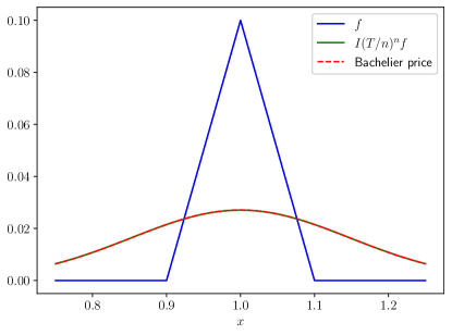
Figure 1. Convergence of the binomial model to the Bachelier model for a butterfly option⁵. Maturity: $T=0.5$; number of time steps: $n=200$; parameters of the process: $\sigma=20\%$, $\mu=5\%$; risk aversion: $\alpha=1$.

Figure 1 shows the convergence of the binomial models to the Bachelier model for a butterfly option with maturity $T=0.5$ (6 months) starting from a binomial model with volatility $\sigma=20\%$ and drift $\mu=5\%$.

4.3. Several linear models

The observation that the risk aversion parameter does not affect the pricing dynamics extends to any linear model. Indeed, for $\Theta:={\mathbb{R}^{d}}$ and any linear expectation $\mathcal{E}[\cdot]:=\mathbb{E}_{\mathbb{P}}[\cdot]$, Corollary 3.4 guarantees that the generator is given by

$$(Af)(x)=\frac{1}{2}\mathbb{E}_{\mathbb{P}}\big{[}\zeta^{T}D^{2}f(x)\zeta\big{]}\quad\mbox{for all }f\in{\rm C}_{\rm b}^{2}\mbox{ and }x\in{\mathbb{R}^{d}}.$$

Furthermore, as long as the models share the same covariance structure given by the function $G(a):=\mathbb{E}[\zeta^{T}a\zeta]$ for all $a\in\mathbb{R}^{d\times d}$, the semigroup $(S(t))_{t\geq 0}$ does not depend on the particular choice of the distribution $\mathbb{P}\circ\zeta^{-1}$.

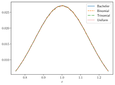
(a) Pricing dynamics

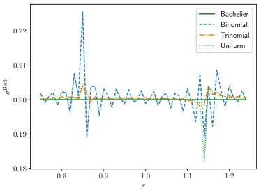
(b) Implied Bachelier volatilities

Figure 2. Convergence of several linear models to the Bachelier model for a butterfly option⁵; Parameters: $n=100$, $\sigma=20\%$, $\mu=5\%$, $\alpha=1$. Figure (a) displays the pricing functional for the maturity $T=0.5$; figure (b) shows the corresponding Bachelier implied volatilities.

Figure 2 shows the approximation of the same risk-based prices with different linear models having the same volatility ($\sigma=20\%$). We compare the following models:

(Binomial) $$\qquad\mathbb{E}_{\mathbb{P}}[f(\zeta)]=\frac{1}{2}\big{(}f(\sigma)+f(-\sigma)\big{)},$$

(Trinomial) $$\qquad\mathbb{E}_{\mathbb{P}}[f(\zeta)]=\frac{1}{3}\big{(}f(\sqrt{3/2}\sigma)+f(0)+f(-\sqrt{3/2}\sigma)\big{)},$$

(Uniform) $$\qquad\mathbb{E}_{\mathbb{P}}[f(\zeta)]=\frac{1}{2\sigma\sqrt{3}}\int_{-\sigma\sqrt{3}}^{\sigma\sqrt{3}}f(x)\,{\rm d}x.$$

While all these models converge to the same Bachelier price, it seems that richer models convergence faster when using the same number of steps in the time discretization. This is particularly evident from the plot of the Bachelier implied volatilities.

4.4. Uncertain binomial model

We consider a one-dimensional binomial model with drift $\mu\in\mathbb{R}$ and volatility uncertainty. Using the parametrization from Example 2.1(ii), we choose $\nu:=\delta_{0}$ and $\Lambda:=[\sigma_{0}-u,\sigma_{0}+u]$, where $\sigma_{0}>0$ is a reference volatility and $u\in[0,\sigma_{0}]$ is the level of uncertainty. This yields the sublinear expectation

$$\mathcal{E}[f(\zeta)]:=\sup_{\sigma\in[\sigma_{0}-u,\sigma_{0}+u]}\frac{1}{2}\big{(}f(\sigma)+f(-\sigma)\big{)}\quad\mbox{for all }f\in{\rm C}_{\rm b}.$$

Here, the risk averse agent fears the worst-case and increases the price as it can be seen in Figure 3.

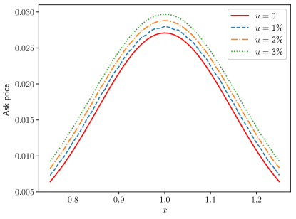
Figure 3. Impact of the level of uncertainty on the risk-based ask price for a butterfly option⁵. Parameters: $T=0.5$, $n=100$, $\mu=5\%$, $\sigma_{0}=20\%$, $\alpha=1$.

Moreover, condition (3.12) is satisfied for any $u\in[0,\sigma_{0})$ in which case Theorem 3.6 implies that the risk-based prices convergence to the $G$-expectation as $\alpha\to\infty$. Figure 4a displays the worst-case bound given by the $G$-expectation and the risk-based prices for different levels of risk aversion. As shown in Corollary 3.4, the risk-based prices are always lower than the worst-case ones. Figure 4b shows more in detail how the risk-based prices approach the $G$-expectation as the risk aversion parameter increases. Recall from Subsection 2.2 that the $G$-expectation is obtained by a Chernoff-type approximation with one-step operator $(J(t)f)(x):=\mathcal{E}[f(x+\sqrt{t}\zeta)]$.

(a) Payoff and ask prices

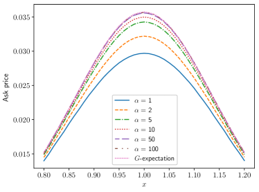
(b) Focus on the risk aversion

Figure 4. Impact of the risk aversion parameter on the risk-based ask price for a butterfly option⁵ and comparison with the worst-case bound. Parameters: $T=0.5$, $n=100$, $\mu=5\%$, $\sigma_{0}=20\%$, $u=3\%$. Figure (a) also displays the payoff function while figure (b) shows more levels of risk aversion.

4.5. Bid-ask spread

Using the same arguments as in Section 3, we can additionally define bid pricing operators. Indeed, switching to the buyer position, we obtain that the one-step bid prices $b_{h,X_{t}^{h}}(f)$ have to satisfy the indifference pricing relation

$$\inf_{\theta\in\Theta}\rho\big{[}b_{h,X_{t}^{h}}(f)-f(X_{t+h}^{x})-\theta^{T}\big{(}X_{t+h}^{x}-X_{t}^{x}\big{)}\big{]}=\inf_{\theta\in\Theta}\rho\big{[}-\theta^{T}\big{(}X_{t+h}^{x}-X_{t}^{x}\big{)}\big{]}.$$

Hence, similarly to equation (3.2), we can define the one-step pricing operators

$$(J(t)f)(x):=b_{t,x}(f)=\tilde{\rho}_{t,x}[0]-\tilde{\rho}_{t,x}[-f]=-\big{(}I(t)(-f)\big{)}(x)$$

and the corresponding time consistent multi-step pricing operators

$$b_{kh,x}^{k}:=(J(h)^{k}f)(x)=-\big{(}I(h)^{k}(-f)\big{)}(x)=-a_{kh,x}^{k}(-f)$$

for all $f\in{\rm C}_{\rm b}$, $x\in{\mathbb{R}^{d}}$ and $k\in\mathbb{N}$. Consequently, for every $t\geq 0$ and $h_{n}:=t/n$, the limit

$$b_{t,x}^{\infty}(f):=\lim_{n\to\infty}b_{nh_{n},x}^{n}(f)=\lim_{n\to\infty}-a_{nh_{n},x}^{n}(-f)=-a_{t,x}^{\infty}(-f)$$

exists and satisfies $b_{t,x}^{\infty}(f)\leq a_{t,x}^{\infty}(f)$ for all $f\in{\rm C}_{\rm b}$ and $x\in{\mathbb{R}^{d}}$. Hence, in the absence of trading constraints, Corollary 3.4 implies that the bid-ask spread for the risk-based prices is smaller than the bid-ask spread for the worst-case prices associated to the $G$-expectation. We now consider again the uncertain binomial model from Subsection 4.4 with reference volatility $\sigma_{0}=20\%$ and uncertainty level $u=3\%$.

(a) Payoff and bid prices

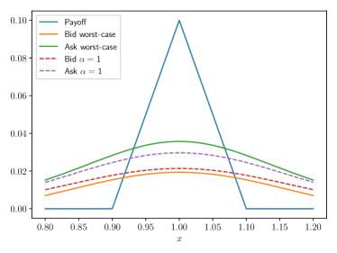
(b) Risk-based bounds vs worst-case bounds

Figure 5. (a) Impact of the risk aversion on the risk-based bid price for a butterfly option⁵. (b) Comparison of the risk-based bid-ask bounds with the worst-case bid-ask bounds. Parameters: $T=0.5$, $n=100$, $\mu=5\%$, $\sigma_{0}=20\%$, $u=3\%$.

Figure 5a shows the bid prices at different levels of risk aversion for a butterfly option⁵ while Figure 5b compares the risk-based bid-ask bounds with the worst-case ones corresponding to pricing with a $G$-expectation. The risk-based approach, which considers the attitude of the agent towards uncertainty, clearly leads to a reduction of the bid-ask spread.

5. Proof of the main results

In order to prove Theorem 3.2 and Theorem 3.3, we rely on the following results from [18].

Definition 5.1.

Let $(I(t))_{t\geq 0}$ be a family of operators $I(t)\colon{\rm C}_{\rm b}\to{\rm C}_{\rm b}$. The Lipschitz set $\mathcal{L}_{I}$ consists of all $f\in{\rm C}_{\rm b}$ such that there exist $c\geq 0$ and $t_{0}>0$ with

$$\|I(t)f-f\|_{\infty}\leq ct\quad\mbox{for all }t\in[0,t_{0}].$$

Moreover, for every $f\in{\rm C}_{\rm b}$ such that the following limit exists, we define

$$I^{\prime}(0)f:=\lim_{h\downarrow 0}\frac{I(h)f-f}{h}\in{\rm C}_{\rm b}.$$

Recall that all limits in ${\rm C}_{\rm b}$ are taken w.r.t. the mixed topology.

Assumption 5.2.

Let $(I(t))_{t\geq 0}$ be a family of operators $I(t)\colon{\rm C}_{\rm b}\to{\rm C}_{\rm b}$ satisfying the following conditions:

1. $I(0)=\operatorname{id}_{{\rm C}_{\rm b}}$.

2. $I(t)$ is convex and monotone with $I(t)0=0$ for all $t\geq 0$.

3. There exists $\omega\geq 0$ with

   $$\|I(t)f-I(t)g\|_{\infty}\leq e^{\omega t}\|f-g\|_{\infty}\quad\mbox{for all }t\in[0,1]\mbox{ and }f,g\in{\rm C}_{\rm b}.$$

4. For every $\varepsilon>0$, there exist $t_{0}>0$ and $\delta>0$ with

   $$I(t)(\tau_{x}f)\leq\tau_{x}I(t)f+r\varepsilon t$$

   for all $t\in[0,t_{0}]$, $x\in B_{{\mathbb{R}^{d}}}(\delta)$, $r\geq 0$ and $f\in{\rm Lip}_{\rm b}(r)$.

5. The limit $I^{\prime}(0)f\in{\rm C}_{\rm b}$ exists for all $f\in{\rm C}_{\rm b}^{\infty}$.

6. For every $T\geq 0$, $K\Subset{\mathbb{R}^{d}}$ and $(f_{k})_{k\in\mathbb{N}}\subset{\rm C}_{\rm b}$ with $f_{k}\downarrow 0$,

   $$\sup_{(t,x)\in[0,T]\times K}\sup_{n\in\mathbb{N}}\big{(}I\big{(}\tfrac{t}{n}\big{)}^{n}f_{k}\big{)}(x)\downarrow 0\quad\mbox{as }k\to\infty.$$

7. It holds $I(t)\colon{\rm Lip}_{\rm b}(r)\to{\rm Lip}_{\rm b}(e^{\omega t}r)$ for all $r,t\geq 0$.

The previous conditions guarantee that [18, Assumption 5.7] is satisfied since condition (vi) is equivalent to [18, Assumption 5.7(vi)], see [18, Lemma C.2]. Hence, the next theorem follows immediately from [18, Theorem 5.4, Theorem 5.9 and Corollary 5.11].

Theorem 5.3.

Let $(I(t))_{t\geq 0}$ be a family of operators $I(t)\colon{\rm C}_{\rm b}\to{\rm C}_{\rm b}$ satisfying Assumption 5.2. Then, there exists a strongly continuous convex monotone semigroup $(S(t))_{t\geq 0}$ on ${\rm C}_{\rm b}$ which is given by

$$S(t)f:=\lim_{n\to\infty}I\big{(}\tfrac{t}{n}\big{)}^{n}f\quad\mbox{for all }t\geq 0\mbox{ and }f\in{\rm C}_{\rm b}.$$ (5.1)

In addition, the following statements are valid:

1. It holds $f\in D(A)$ and $Af=I^{\prime}(0)f$ for all $f\in{\rm C}_{\rm b}$ such that $I^{\prime}(0)f\in{\rm C}_{\rm b}$ exists. In particular, this is valid for all $f\in{\rm C}_{\rm b}^{\infty}$.

2. It holds $\|S(t)f-S(t)g\|_{\infty}\leq e^{\omega t}\|f-g\|_{\infty}$ for all $t\geq 0$ and $f,g\in{\rm C}_{\rm b}$.

3. For every $\varepsilon>0$, $r,T\geq 0$ and $K\Subset\mathbb{R}^{d}$, there exist $K^{\prime}\Subset\mathbb{R}^{d}$ and $c\geq 0$ with

   $$\|S(t)f-S(t)g\|_{\infty,K}\leq c\|f-g\|_{\infty,K^{\prime}}+\varepsilon$$

   for all $t\in[0,T]$ and $f,g\in B_{{\rm C}_{\rm b}}(r)$.

4. It holds $\mathcal{L}_{I}\subset\mathcal{L}_{S}$ and $S(t)\colon\mathcal{L}_{S}\to\mathcal{L}_{S}$ for all $t\geq 0$.

5. For every $\varepsilon>0$, there exists $\delta>0$ with

   $$S(t)(\tau_{x}f)\leq\tau_{x}S(t)f+e^{\omega t}r\varepsilon t$$

   for all $r,t\geq 0$, $f\in{\rm Lip}_{\rm b}(r)$ and $x\in B_{\mathbb{R}^{d}}(\delta)$.

6. It holds $S(t)\colon{\rm Lip}_{\rm b}(r)\to{\rm Lip}_{\rm b}(e^{\omega t}r)$ for all $r,t\geq 0$.

It follows from [18, Theorem 4.7] that semigroups which have been constructed this way are uniquely determined by their generators evaluated at smooth functions.

Theorem 5.4.

Let $(S(t))_{t\geq 0}$ and $(T(t))_{t\geq 0}$ be two strongly continuous convex monotone semigroups on ${\rm C}_{\rm b}$ with generators $A$ and $B$, respectively, which satisfy the conditions (v) and (vi) of Theorem 5.3. Furthermore, we assume that ${\rm C}_{\rm b}^{\infty}\subset D(A)\cap D(B)$ and

$$Af\leq Bf\quad\mbox{for all }f\in{\rm C}_{\rm b}^{\infty}.$$

Then, it holds $S(t)f\leq T(t)f$ for all $t\geq 0$ and $f\in{\rm C}_{\rm b}$.

5.1. Proof of Theorem 3.2

Recall that

$$(I_{R}(t)f)(x):=\inf_{\theta\in\Theta_{R}}\rho[f(x+\zeta_{t})-\theta^{T}\zeta_{t}]-c_{R}(t),$$

for all $R,t\geq 0$, $f\in{\rm C}_{\rm b}$ and $x\in{\mathbb{R}^{d}}$, where $\zeta_{t}:=t\mu+\sqrt{t}\zeta$ and $c_{R}(t):=\inf_{\theta\in\Theta_{R}}\rho[-\theta^{T}\zeta_{t}]$. In the sequel, we fix $R\geq 0$ and therefore simply write $I(t)f:=I_{R}(t)f$, $S(t)f:=S_{R}(t)f$, $Af:=A_{R}f$, $\Theta:=\Theta_{R}$ and $c(t):=c_{R}(t)$.

Proof of Theorem 3.2.

In order to apply Theorem 5.3, we have to verify Assumption 5.2. Furthermore, we have to show that

$$(I^{\prime}(0)f)(x)=\inf_{\theta\in\Theta}G_{\theta}(D^{2}f(x),Df(x))-\inf_{\theta\in\Theta}G_{\theta}(0,0)\quad\mbox{for all }f\in{\rm C}_{\rm b}^{2}\mbox{ and }x\in{\mathbb{R}^{d}},$$

where $G_{\theta}$ is defined by equation (3.6). First, we verify Assumption 5.2(i)-(iv) and (vii). Condition (i) follows from $\zeta_{0}\equiv 0$. Regarding condition (ii), the monotonicity of $\rho$ yields the monotonicity of $I(t)$ and $I(t)0=0$ holds by definition. Let $\lambda\in[0,1]$, $f_{1},f_{2}\in{\rm C}_{\rm b}$, $x\in{\mathbb{R}^{d}}$ and $\varepsilon>0$. Let $\theta_{1},\theta_{2}\in\Theta$ be $\varepsilon$-optimizers of $(I(t)f_{1})(x)$ and $(I(t)f_{2})(x)$, respectively, and define $\tilde{f}=\lambda f_{1}+(1-\lambda)f_{2}\in{\rm C}_{\rm b}$ and $\tilde{\theta}=\lambda\theta_{1}+(1-\lambda)\theta_{2}\in\Theta$. Then, by convexity of $\rho$,

$$\big{(}I(t)\tilde{f}\big{)}(x) \leq\rho\big{[}\tilde{f}(x+\zeta_{t})+\tilde{\theta}^{T}\zeta_{t}\big{]}-c(t)$$

$$\leq\lambda\big{(}\rho\big{[}f_{1}(x+\zeta_{t})+\theta_{1}^{T}\zeta_{t}\big{]}-c(t)\big{)}+(1-\lambda)\big{(}\rho\big{[}f_{2}(x+\zeta_{t})+\theta_{2}^{T}\zeta_{t}\big{]}-c(t)\big{)}$$

$$=\lambda(I(t)f_{1})(x)+(1-\lambda)(I(t)f_{2})(x)+\varepsilon.$$

Letting $\varepsilon\downarrow 0$ shows that $I(t)$ is convex. For every $t\geq 0$, $f,g\in{\rm C}_{\rm b}$, $x\in{\mathbb{R}^{d}}$ and $\theta\in\Theta$, the monotonicity and cash invariance of $\rho$ imply

$$(I(t)f)(x)\leq\rho\big{[}f(x+\zeta_{t})+\theta^{T}\zeta_{t}\big{]}-c(t)\leq\rho\big{[}g(x+\zeta_{t})+\theta^{T}\zeta_{t}\big{]}-c(t)+\|f-g\|_{\infty}.$$

Taking the infimum over $\theta\in\Theta$ and changing the roles of $f$ and $g$ yields

$$\|I(t)f-I(t)g\|_{\infty}\leq\|f-g\|_{\infty}\quad\mbox{for all }t\geq 0$$

which shows that condition (iii) is satisfied with $\omega:=0$. Condition (iv) follows from

$$I(t)(\tau_{x}f)=\tau_{x}I(t)f\quad\mbox{for all }t\geq 0,f\in{\rm C}_{\rm b}\mbox{ and }x\in{\mathbb{R}^{d}}.$$

In order to verify condition (vii) with $\omega:=0$, we observe that

$$|(I(t)f)(x)-(I(t)f)(y)| =|(\tau_{x}I(t)f)(0)-(\tau_{y}I(t)f)(0)|=|(I(t)\tau_{x}f)(0)-(I(t)\tau_{y}f)(0)|$$

$$\leq\|\tau_{x}f-\tau_{y}f\|_{\infty}\leq r|x-y|$$

for all $r,t\geq 0$, $f\in{\rm Lip}_{b}(r)$ and $x\in{\mathbb{R}^{d}}$.

Second, we show that ${\rm C}_{\rm b}^{2}\subset\mathcal{L}_{I}$. Let $f\in{\rm C}_{\rm b}^{2}$. For every $t\in[0,1]$, $x\in{\mathbb{R}^{d}}$ and $\theta\in\Theta$, applying Taylor’s formula on the function $g(y):=\exp(\alpha(f(x+y)-f(x))-\alpha\theta^{T}y)$ yields

$$\exp\big{(}\alpha(f(x+\zeta_{t})-f(x))-\alpha\theta^{T}\zeta_{t}\big{)}=1+\alpha(Df(x)-\theta)^{T}\zeta_{t}$$

$$\quad\;+\int_{0}^{1}\big{(}\alpha^{2}|(Df(x+s\zeta_{t})-\theta)^{T}\zeta_{t}|^{2}+\alpha\zeta_{t}^{T}D^{2}f(x+s\zeta_{t})\zeta_{t}\big{)}g(s\zeta_{t})(1-s)\,{\rm d}s.$$ (5.2)

It follows from Assumption 3.1 and Lemma A.2(vi) that

$$\big{|}\mathcal{E}\big{[}\exp(\alpha(f(x+\zeta_{t})-f(x))-\alpha\theta^{T}\zeta_{t})\big{]}-1\big{|}$$

$$\leq\alpha(\|Df\|_{\infty}+R)|\mu|t+\frac{\alpha}{2}\mathcal{E}\left[\big{(}\alpha(\|Df\|_{\infty}+R)^{2}+\|D^{2}f\|_{\infty}\big{)}|\zeta_{t}|^{2}e^{2\alpha\|f\|_{\infty}+\alpha R|\zeta_{t}|}\right]$$

$$\leq\alpha(\|Df\|_{\infty}+R)|\mu|t$$

$$\quad\;+\frac{\alpha}{2}\mathcal{E}\left[\big{(}\alpha(\|Df\|_{\infty}+R)^{2}+\|D^{2}f\|_{\infty}\big{)}\big{(}|\mu|^{2}+2|\mu|\cdot|\zeta|+|\zeta|^{2}\big{)}e^{\alpha(2\|f\|_{\infty}+R(|\mu|+|\zeta|))}\right]t$$

for all $t\in[0,1]$, $x\in{\mathbb{R}^{d}}$ and $\theta\in\Theta$. Hence, there exist $c_{1},c_{2}\geq 0$ and $t_{0}>$ with

$$-c_{2}t\leq\log(1-c_{1}t)\leq\log\big{(}\mathcal{E}\big{[}\exp(\alpha f(x+\zeta_{t})-\alpha\theta^{T}\zeta_{t}\big{]}\big{)}-f(x)\leq\log(1+c_{1}t)\leq c_{2}t$$

for all $t\in[0,t_{0}]$, $x\in{\mathbb{R}^{d}}$ and $\theta\in\Theta$. Dividing by $\alpha>0$, taking the supremum over $\theta\in\Theta$ and applying the previous estimate with $f\equiv 0$ shows that

$$\|I(t)f-f\|_{\infty}\leq\sup_{\theta\in\Theta}\big{\|}\rho\big{[}f(\,\cdot\,+\zeta_{t})-\theta^{T}\zeta_{t}\big{]}-f\big{\|}_{\infty}+\sup_{\theta\in\Theta}\big{|}\rho\big{[}-\theta^{T}\zeta_{t}\big{]}\big{|}\leq 2c_{2}t\quad\mbox{for all }t\in[0,t_{0}].$$

Third, we verify condition (vi). Several sufficient conditions which guarantee that condition (vi) is valid have been systemically explored in [22, Subsection 2.5]. Here, we show that, for every $r\geq 0$, there exists $c\geq 0$ with

$$\|I(t)f-f\|_{\infty}\leq c\big{(}\|Df\|_{\infty}+\|D^{2}f\|_{\infty}\big{)}t$$ (5.3)

for all $t\in[0,1]$ and $f\in{\rm C}_{\rm b}^{2}$ with $\|f\|_{\infty}\leq r$ and $\|Df\|_{\infty}+\|D^{2}f\|_{\infty}\leq 1$. Let $r\geq 0$, $t\in[0,1]$ and $f\in{\rm C}_{\rm b}^{2}$ with $\|f\|_{\infty}\leq r$ and $0<\|Df\|_{\infty}+\|D^{2}f\|_{\infty}\leq 1$. For every $\lambda\in(0,1)$, $x\in{\mathbb{R}^{d}}$ and $\theta\in\Theta$, applying equation (5.2) with $\frac{1}{\lambda}f$ yields

$$\mathcal{E}\left[\exp\left(\frac{\alpha(f(x+\zeta_{t})-f(x))}{\lambda}-\alpha\theta^{T}\zeta_{t}\right)\right]$$

$$\leq 1+\alpha\big{(}\tfrac{1}{\lambda}\|Df\|_{\infty}+R\big{)}|\mu|t$$

$$\quad\;+\alpha\mathcal{E}\left[\int_{0}^{1}\Big{(}\tfrac{\alpha}{\lambda^{2}}\|Df\|_{\infty}^{2}+\tfrac{\alpha}{\lambda}\|Df\|_{\infty}R+\alpha R^{2}+\tfrac{1}{\lambda}\|D^{2}f\|_{\infty}\Big{)}|\zeta_{t}|^{2}g(sX_{s})(1-s)\,{\rm d}s\right].$$

We apply Lemma A.1 with $\lambda:=\|Df\|_{\infty}+\|D^{2}f\|_{\infty}\in(0,1]$ to obtain

$$\rho\big{[}f(x+\zeta_{t})-f(x)-\theta^{T}\zeta_{t}\big{]}-\rho\big{[}-\theta^{T}\zeta_{t}\big{]}\leq\lambda\rho\left[\frac{f(x+\zeta_{t})-f(x)}{\lambda}-\theta^{T}\zeta_{t}\right]-\lambda\rho\big{[}-\theta^{T}\zeta_{t}\big{]}$$

$$\leq\frac{\lambda}{\alpha}\log\left(1+\alpha(1+R)|\mu|t+\frac{\alpha^{2}(1+R+R^{2})+\alpha)}{2}\mathcal{E}\left[|\zeta_{t}|^{2}e^{\alpha(2r+R|\zeta_{t}|)}\right]\right)$$

$$\quad\;+\frac{\lambda}{\alpha}\log\left(1+\alpha R|\mu|t+\frac{\alpha^{2}R^{2}}{2}\mathcal{E}\left[|\zeta_{t}|^{2}e^{\alpha R|\zeta_{t}|}\right]\right)$$

$$\leq\frac{\lambda}{\alpha}\log\big{(}1+\alpha(1+R)|\mu|t+\mathcal{E}[Y]t\big{)}+\frac{\lambda}{\alpha}\log\big{(}1+\alpha R|\mu|t+\mathcal{E}[Z]t\big{)}$$

for all $x\in{\mathbb{R}^{d}}$ and $\theta\in\Theta$, where

$$Y :=\tfrac{1}{2}\big{(}\alpha^{2}(1+R+R^{2})+\alpha\big{)}\big{(}|\mu|^{2}+2|\mu|\cdot|\zeta|+|\zeta|^{2}\big{)}e^{\alpha(2r+R(|\mu|+|\zeta|))},$$

$$Z :=\tfrac{1}{2}\alpha^{2}R^{2}\big{(}|\mu|^{2}+2|\mu|\cdot|\zeta|+|\zeta|^{2}\big{)}e^{\alpha R(|\mu|+|\zeta|)}.$$

The lower bound follows similarly and therefore taking the supremum over $\theta\in\Theta$ shows that, for every $r\geq 0$, there exists $c\geq 0$ with

$$|(I(t)f-f)(x)| =\Big{|}\inf_{\theta\in\Theta}\rho[f(x+\zeta_{t})-\theta^{T}\zeta_{t}]-\inf_{\theta\in\Theta}\rho[-\theta^{T}\zeta_{t}]\Big{|}$$

$$\leq\sup_{\theta\in\Theta}\big{|}\rho\big{[}f(x+\zeta_{t})-f(x)-\theta^{T}\zeta_{t}\big{]}-\rho\big{[}-\theta^{T}\zeta_{t}\big{]}\big{|}\leq c\big{(}\|Df\|_{\infty}+\|D^{2}f\|_{\infty}\big{)}t$$

for all $t\in[0,1]$, $f\in{\rm C}_{\rm b}^{2}$ with $\|f\|_{\infty}\leq r$ and $0<\|Df\|_{\infty}+\|D^{2}f\|_{\infty}\leq 1$ and $x\in{\mathbb{R}^{d}}$. Hence, we can apply [22, Corollary 2.14] with $S_{n}(t)f:=I(\frac{t}{n})^{n}f$, $\mathcal{T}_{n}:=\mathbb{R}_{+}$ and $X_{n}:={\mathbb{R}^{d}}$ for all $t\geq 0$, $f\in{\rm C}_{\rm b}$ and $n\in\mathbb{N}$ to obtain that condition (vi) is satisfied.

Fourth, for every $f\in{\rm C}_{\rm b}^{2}$, we show that the limit $I^{\prime}(0)f\in{\rm C}_{\rm b}$ exists and is given by

$$(I^{\prime}(0)f)(x)=\inf_{\theta\in\Theta}G_{\theta}(D^{2}f(x),Df(x))-\inf_{\theta\in\Theta}G_{\theta}(0,0)\quad\mbox{for all }x\in{\mathbb{R}^{d}},$$

where $G_{\theta}(a,b)=\frac{1}{2}\mathcal{E}[\zeta^{T}a\zeta+\alpha|(b-\theta)^{T}\zeta|^{2}]+(b-\theta)^{T}\mu$ for all $a\in\mathbb{R}^{d\times d}$, $b\in{\mathbb{R}^{d}}$ and $\theta\in\Theta$. Let $f\in{\rm C}_{\rm b}^{2}$. Equation (5.2), Assumption 3.1 and Lemma A.2(i) and (vi) imply

$$\frac{1}{\alpha t}\log\big{(}\mathcal{E}\big{[}\exp\big{(}\alpha(f(x+\zeta_{t})-f(x))-\alpha\theta^{T}\zeta_{t}\big{)}\big{]}\big{)}-G_{\theta}(D^{2}f(x),Df(x))$$

$$=\frac{1}{\alpha t}\log\big{(}1+\alpha(Df(x)-\theta)^{T}\mu t+\mathcal{E}[Y_{t}^{\theta,x}]\big{)}-(Df(x)-\theta)^{T}\mu$$

$$\quad\;-\frac{1}{2}\mathcal{E}\left[\alpha|(Df(x)-\theta)^{T}\zeta|^{2}+\zeta^{T}D^{2}f(x)\zeta\big{)}\right]$$

$$=\frac{1}{\alpha t}\mathcal{E}[Y_{t}^{\theta,x}]-\mathcal{E}[Z^{\theta,x}]+r_{t}^{\theta,x}$$ (5.4)

for all $t>0$, $x\in{\mathbb{R}^{d}}$ and $\theta\in\Theta$, where

$$Y_{t}^{\theta,x} :=\int_{0}^{1}\big{(}\alpha^{2}|(Df(x+s\zeta_{t})-\theta)^{T}\zeta_{t}|^{2}+\alpha\zeta_{t}^{T}D^{2}f(x+s\zeta_{t})\zeta_{t}\big{)}g^{\theta,x}(s\zeta_{t})(1-s)\,{\rm d}s,$$

$$Z^{\theta,x} :=\frac{1}{2}\alpha|(Df(x)-\theta)^{T}\zeta|^{2}+\frac{1}{2}\zeta^{T}D^{2}f(x)\zeta,$$

$$r_{t}^{\theta,x} :=\frac{1}{\alpha t}\log\big{(}1+\alpha(Df(x)-\theta)^{T}\mu t+\mathcal{E}[Y_{t}^{\theta,x}]\big{)}-\Big{(}(Df(x)-\theta)^{T}\mu+\frac{1}{\alpha t}\mathcal{E}[Y_{t}^{\theta,x}]\big{)}\Big{)}$$

and $g^{\theta,x}\colon{\mathbb{R}^{d}}\to\mathbb{R},\;y\mapsto\exp(\alpha(f(x+y)-f(x))-\alpha\theta^{T}y)$. For every $t\in(0,1]$, $x\in{\mathbb{R}^{d}}$ and $\theta\in\Theta$, we can estimate

$$|\alpha(Df(x)-\theta)^{T}\mu t|\leq\alpha(\|Df\|_{\infty}+R)|\mu|t$$

and, by defining $c_{f}:=\alpha^{2}(\|Df\|_{\infty}+R)^{2}+\alpha\|D^{2}f\|_{\infty}$,

$$\mathcal{E}[|Y_{t}^{\theta,x}|] \leq\mathcal{E}\left[\frac{1}{2}\big{(}\alpha^{2}(\|Df\|_{\infty}+R)^{2}+\alpha\|D^{2}f\|_{\infty}\big{)}|\zeta_{t}|^{2}e^{\alpha(2\|f\|_{\infty}+R|\zeta_{t}|)}\right]$$

$$\leq\mathcal{E}\left[\frac{\alpha}{2}c_{f}\big{(}|\mu|^{2}+2|\mu|\cdot|\zeta|+|\zeta|^{2}\big{)}e^{\alpha(2\|f\|_{\infty}+R(|\mu|+|\zeta|))}\right]t.$$ (5.5)

Since $\log(1+z)=z+o(|z|)$ for $z\to 0$, we obtain

$$\sup_{x\in{\mathbb{R}^{d}}}\sup_{\theta\in\Theta}|r_{t}^{\theta,x}|\to 0\quad\mbox{as }t\downarrow 0.$$ (5.6)

It remains to show that, for every $K\Subset{\mathbb{R}^{d}}$,

$$\sup_{x\in K}\sup_{\theta\in\Theta}\left|\frac{1}{\alpha t}\mathcal{E}[Y_{t}^{\theta,x}]-\mathcal{E}[Z^{\theta,x}]\right|\to 0\quad\mbox{as }t\downarrow 0.$$ (5.7)

For every $t\in(0,1]$, $x\in{\mathbb{R}^{d}}$ and $\theta\in\Theta$, Lemma A.2(viii) implies

$$\left|\frac{1}{\alpha t}\mathcal{E}[Y_{t}^{\theta,x}]-\mathcal{E}[Z^{\theta,x}]\right|\leq\mathcal{E}\left[\left|\frac{1}{\alpha t}Y_{t}^{\theta,x}-Z^{\theta,x}\right|\right].$$

Moreover, for every $\varepsilon>0$, by inequality (5.1) and Assumption 3.1, there exists $c\geq 0$ with

$$\mathcal{E}\left[\left|\frac{1}{\alpha t}Y_{t}^{\theta,x}-Z^{\theta,x}\right|\mathds{1}_{\{|\zeta|>c\}}\right]\leq\varepsilon\quad\mbox{for all }t\in(0,1],x\in{\mathbb{R}^{d}}\mbox{ and }\theta\in\Theta.$$ (5.8)

Let $\varepsilon>0$ and choose $c\geq 0$ such that the previous inequality is valid. It follows from

$$|\zeta_{t}|^{2}=(t|\mu|^{2}+2\sqrt{t}\mu^{T}\zeta+|\zeta|^{2})t$$

that there exists $C\geq 0$ with

$$\mathcal{E}\left[\left|\frac{1}{\alpha t}Y_{t}^{\theta,x}-Z^{\theta,x}\right|\mathds{1}_{\{|\zeta|\leq c\}}\right]$$

$$\leq\alpha\mathcal{E}\left[\int_{0}^{1}\big{(}|(Df(x+s\zeta_{t})-\theta)^{T}\zeta|^{2}-|(Df(x)-\theta)^{T}\zeta|^{2}\big{)}\mathds{1}_{\{\zeta|\leq c\}}(1-s)\,{\rm d}s\right]$$

$$\quad\;+\mathcal{E}\left[\int_{0}^{1}\big{(}|\zeta^{T}D^{2}f(x+s\zeta_{t})\zeta g^{\theta,x}(s\zeta_{t})-\zeta^{T}D^{2}f(x)\zeta\big{)}\mathds{1}_{\{\zeta|\leq c\}}(1-s)\,{\rm d}s\right]+C\sqrt{t}$$

for all $t\in(0,1]$, $x\in{\mathbb{R}^{d}}$ and $\theta\in\Theta$. Let $K\Subset{\mathbb{R}^{d}}$. Since the functions $\{g^{\theta,x}\colon\theta\in\Theta,x\in K\}$ are equicontinuous with $g^{\theta,x}(0)=1$ and $\zeta_{t}\mathds{1}_{\{|\zeta|\leq c\}}$ converges uniformly to zero as $t\downarrow 0$, there exists $t_{0}\in(0,1]$ with

$$\mathcal{E}\left[\left|\frac{1}{\alpha t}Y_{t}^{\theta,x}-Z^{\theta,x}\right|\mathds{1}_{\{|\zeta|\leq c\}}\right]\leq\varepsilon\quad\mbox{for all }t\in(0,t_{0}],x\in K\mbox{ and }\theta\in\Theta.$$ (5.9)

Combining the inequalities (5.8) and (5.9) shows that equation (5.7) is valid. Hence, it follows from equation (5.4) that

$$\sup_{x\in K}\left|\frac{1}{t}\Big{(}\inf_{\theta\in\Theta}\rho[f(x+\zeta_{t})-\theta^{T}\zeta_{t}]-f(x)\Big{)}-\inf_{\theta\in\Theta}G_{\theta}(D^{2}f(x),Df(x))\right|$$

$$\leq\sup_{x\in K}\sup_{\theta\in\Theta}\frac{1}{\alpha t}\big{|}\log\big{(}\mathcal{E}\big{[}\exp\big{(}\alpha(f(x+\zeta_{t})-f(x))-\alpha\theta^{T}\zeta_{t}\big{)}\big{]}\big{)}-G_{\theta}(D^{2}f(x),Df(x))\big{|}$$

$$\leq\sup_{x\in K}\sup_{\theta\in\Theta}\left|\frac{1}{\alpha t}\mathcal{E}[Y_{t}^{\theta,x}]-\mathcal{E}[Z^{\theta,x}]+r_{t}^{\theta,x}\right|\to 0\quad\mbox{as }t\downarrow 0.$$

By additionally applying this result on the constant function $f\equiv 0$, we obtain that the limit $I^{\prime}(0)f\in{\rm C}_{\rm b}$ exists and is given by

$$(I^{\prime}(0)f)(x)=\inf_{\theta\in\Theta}G_{\theta}(D^{2}f(x),Df(x))-\inf_{\theta\in\Theta}G_{\theta}(0,0)\quad\mbox{for all }f\in{\rm C}_{\rm b}^{2}\mbox{ and }x\in{\mathbb{R}^{d}}.$$

Now, the claim follows from Theorem 5.3 and Theorem 5.4. ∎

5.2. Proof of Theorem 3.3

The proof is based on the stability results for strongly continuous convex monotone semigroups in [22]. The basic idea is that, for a sequence of semigroups satisfying certain stability conditions, convergence of the generators implies convergence of the corresponding semigroups. In many applications, the generators can be determined explicitly for smooth functions and the same applies to their convergence. In contrast, showing the convergence of the semigroups directly is often not feasible.

Proof of Theorem 3.3.

In order to apply [22, Theorem 2.3], we have to verify [22, Assumption 2.2]. The conditions (i), (iii) and (iv) follow from Theorem 5.3 and the corresponding estimates in the proof of Theorem 3.2. In order to verify the conditions (ii) and (v), we show that, for every $c\geq 0$, there exist $R\geq 0$ and $t_{0}>0$ with

$$\inf_{\theta\in\Theta}G_{\theta}(D^{2}f(x),Df(x))=\inf_{\theta\in\Theta_{R}}G_{\theta}(D^{2}f(x),Df(x))$$ (5.10)

for all $t\in[0,t_{0}]$, $f\in{\rm C}_{\rm b}^{2}$ with $\|Df\|_{\infty}+\|D^{2}f\|_{\infty}\leq c$ and $x\in{\mathbb{R}^{d}}$. Choose $\delta>0$ such that condition (3.8) is satisfied. For every $f\in{\rm C}_{\rm b}^{2}$, $x\in{\mathbb{R}^{d}}$ and $\theta\in\Theta$, Lemma A.2(vii) implies

$$G_{\theta}(D^{2}f(x),Df(x)) =\frac{1}{2}\mathcal{E}\big{[}\alpha|(Df(x)-\theta)^{T}\zeta|^{2}+\zeta^{T}D^{2}f(x)\zeta\big{]}+(Df(x)-\theta)^{T}\mu$$

$$=\frac{1}{2}\mathcal{E}\big{[}\alpha|\theta^{T}\zeta|^{2}-2\alpha Df(x)^{T}\zeta\theta^{T}\zeta+\alpha|Df(x)^{T}\zeta|^{2}+\zeta^{T}D^{2}f(x)\zeta\big{]}$$

$$\quad+(Df(x)-\theta)^{T}\mu$$

$$\geq\frac{\alpha\delta}{2}|\theta|^{2}-c_{1}|\theta|-c_{2},$$

where $c_{1}:=\alpha\|Df\|_{\infty}\mathcal{E}[|\zeta|^{2}]+|\mu|$ and $c_{2}:=\frac{1}{2}(\alpha\|Df\|_{\infty}^{2}+\|D^{2}f\|_{\infty})\mathcal{E}[|\zeta|^{2}]+\|Df\|_{\infty}|\mu|$. This shows that equation (5.10) is valid and condition (v) follows immediately. For $\Theta={\mathbb{R}^{d}}$, we observe that, for every $\theta\in{\mathbb{R}^{d}}$ with $(Df(x)-\theta)^{T}\mu=0$,

$$G_{\theta}(D^{2}f(x),Df(x))\geq\frac{1}{2}\mathcal{E}[\zeta^{T}D^{2}f(x)\zeta]$$

with equality for $\theta=Df(x)$. Moreover, for every $\theta\in{\mathbb{R}^{d}}$ with $(Df(x)-\theta)^{T}\mu\neq 0$, one can use condition (3.9) to estimate

$$G_{\theta}(D^{2}f(x),Df(x))\geq\frac{\alpha\delta}{2}|Df(x)-\theta|^{2}-c_{1}|Df(x)-\theta|-c_{2}$$

for suitable constants $c_{1},c_{2}\geq 0$. Hence, equation (5.10) is still valid for some $R\geq\|Df\|_{\infty}$. In order to verify condition (iii), we further show that there exists $c\geq 0$ with

$$\|A_{R}f\|_{\infty}\leq c\big{(}\|Df\|_{\infty}+\|D^{2}f\|_{\infty}\big{)}$$ (5.11)

for all $f\in{\rm C}_{\rm b}^{2}$ with $\|Df\|_{\infty}+\|D^{2}f\|_{\infty}\leq 1$. By equation (5.10), there exists $R_{0}\geq 0$ with

$$|(A_{R}f)(x)|\leq\sup_{\theta\in\Theta_{R_{0}}}\big{|}G_{\theta}(D^{2}f(x),Df(x))-G_{\theta}(0,0)\big{|}$$

for all $R\geq 0$, $f\in{\rm C}_{\rm b}^{2}$ with $\|Df\|_{\infty}+\|D^{2}f\|_{\infty}\leq 1$ and $x\in{\mathbb{R}^{d}}$. For every $f\in{\rm C}_{\rm b}^{2}$ with $\|Df\|_{\infty}+\|D^{2}f\|_{\infty}\leq 1$, $x\in{\mathbb{R}^{d}}$ and $\theta\in\Theta_{R_{0}}$, it follows from Lemma A.2(viii) that

$$\big{|}G_{\theta}(D^{2}f(x),Df(x))-G_{\theta}(0,0)\big{|}$$

$$=\left|\frac{1}{2}\mathcal{E}\big{[}\zeta^{T}D^{2}f(x)\zeta+\alpha|(Df(x)+\theta)^{T}\zeta|^{2}\big{]}+Df(x)^{T}\mu-\frac{\alpha}{2}\mathcal{E}\left[|\theta^{T}\zeta|^{2}\right]\right|$$

$$\leq\frac{1}{2}\mathcal{E}\big{[}\zeta^{T}D^{2}f(x)\zeta+\alpha|Df(x)^{T}\zeta|^{2}+2\alpha|Df(x)|\cdot|\theta|\cdot|\zeta|^{2}\big{]}+|Df(x)^{T}\mu|$$

$$\leq\frac{1}{2}\big{(}\|D^{2}f\|_{\infty}+\alpha(\|Df\|_{\infty}^{2}+2\|Df\|_{\infty}|\theta|)\big{)}\mathcal{E}[|\zeta|^{2}]+\|Df\|_{\infty}|\mu|$$

$$\leq\left(\frac{1}{2}(1\vee\alpha)(1+2R_{0})\mathcal{E}[|\zeta|^{2}]+|\mu|\right)\big{(}\|Df\|_{\infty}+\|D^{2}f\|_{\infty}\big{)}.$$

This shows that inequality (5.11) is satisfied. Furthermore, it holds

$$\lim_{h\downarrow 0}\left\|\frac{S_{R}(h)f-f}{h}-A_{R}f\right\|_{\infty}=0\quad\mbox{for all }R\geq 0\mbox{ and }f\in\rm BUC^{2},$$

where $\rm BUC^{2}$ denotes the space of all bounded twice differentiable functions $f\colon{\mathbb{R}^{d}}\to\mathbb{R}$ such that the first and second are bounded and uniformly continuous. Indeed, for every $R\geq 0$ and $f\in\rm BUC^{2}$, the supremum in inequality (5.9) and therefore in inequality (5.7) can be taken over $x\in{\mathbb{R}^{d}}$ instead of $x\in K$. We obtain

$$\lim_{h\downarrow 0}\left\|\frac{I_{R}(h)f-f}{h}-I^{\prime}(0)f\right\|_{\infty}=0$$

and [20, Theorem 4.3] transfers the previous statement to the semigroup $(S_{R}(t))_{t\geq 0}$. It follows from [22, Corollary 2.16] that condition (iii) is satisfied for any sequence $R_{n}\to\infty$. The claim now follows from [22, Theorem 2.5] since Theorem 5.4 guarantees that the limit does not depend on the choice of the sequence $R_{n}\to\infty$. ∎

5.3. Proof of Theorem 3.5

The proof is similar to the one of Theorem 3.2 as soon as we can constrain the trading strategies to a bounded set.

Proof.

By condition (3.11), there exists $t_{0}>0$ such that $I(t)$ is well-defined for all $t\in[0,t_{0}]$. Hence, since we are only interested in the limit behaviour of the iterated operators, we can replace $I(t)$ by $I(t_{0})$ for all $t>t_{0}$ without affecting the result. We subsequently show that Assumption 5.2 is satisfied. The conditions (i)-(iv) and (vii) can be verified exactly as in the proof of Theorem 3.2, where we did not use that the set $\Theta=\Theta_{R}$ was bounded. In order to verify condition (v), let $f\in{\rm C}_{\rm b}^{2}$. We show that there exist $R\geq 0$ and $t_{0}>0$ with

$$\inf_{\theta\in{\mathbb{R}^{d}}}\rho[f(x+\zeta_{t})-\theta^{T}\zeta_{t}]=\inf_{|\theta|\leq R}\rho[f(x+\zeta_{t})-\theta^{T}\zeta_{t}]$$ (5.12)

for all $t\in[0,t_{0}]$ and $x\in{\mathbb{R}^{d}}$. For every $t\geq 0$, $x\in{\mathbb{R}^{d}}$ and $\theta\in\Theta$, Taylor’s formula implies

$$f(x+\zeta_{t})=f(x)+Df(x)^{T}\zeta_{t}+\int_{0}^{1}\zeta_{t}^{T}D^{2}f(x+\zeta_{t})\zeta_{t}(1-s)\,{\rm d}s.$$

We choose $\theta=Df(x)$ and apply condition (3.10) to obtain $M\geq 0$ and $t_{1}\in(0,1]$ with

$$\rho[f(x+\zeta_{t})-\theta^{T}\zeta_{t}] =\frac{1}{\alpha}\log\left(\mathcal{E}\left[\exp\left(\alpha f(x)+\alpha\int_{0}^{1}\zeta_{t}^{T}D^{2}f(x+s\zeta_{t})\zeta_{t}(1-s)\,{\rm d}s\right)\right]\right)$$

$$\leq f(x)+\frac{1}{\alpha}\log\big{(}\mathcal{E}\big{[}[e^{2\alpha\|D^{2}f\|_{\infty}(|\mu|^{2}t^{2}+|\zeta|^{2}t)}\big{]}\big{)}$$

$$=f(x)+2(|\mu|^{2}+M)\|D^{2}f\|_{\infty}t$$

for all $t\in[0,t_{1}]$ and $x\in{\mathbb{R}^{d}}$. Furthermore, we apply condition (3.11) with

$$C:=\frac{(4|\mu|^{2}+2M)\|D^{2}f\|_{\infty}+|\mu|}{\sqrt{2\alpha\|D^{2}f\|_{\infty}}}$$

to obtain $R\geq 1$ and $t_{2}\in(0,1]$ with

$$\rho[f(x+\zeta_{t})-\theta^{T}\zeta_{t}]$$

$$=f(x)+(Df(x)-\theta)^{T}\mu t$$

$$\quad\>+\frac{1}{\alpha}\log\left(\mathcal{E}\left[\exp\left(\alpha\sqrt{t}(Df(x)-\theta)^{T}\zeta+\alpha\int_{0}^{1}\zeta_{t}^{T}D^{2}f(x+s\zeta_{t})\zeta_{t}(1-s)\,{\rm d}s\right)\right]\right)$$

$$\geq f(x)+(Df(x)-\theta)^{T}\mu t-2|\mu|^{2}\|D^{2}f\|_{\infty}t^{2}+\frac{1}{\alpha}\log\big{(}\mathcal{E}\big{[}e^{\sqrt{t}\alpha(Df(x)-\theta)^{T}\zeta-2t\alpha\|D^{2}f\|_{\infty}|\zeta|^{2}}\big{]}\big{)}$$

$$\geq f(x)+(Df(x)-\theta)^{T}\mu t-2|\mu|^{2}\|D^{2}f\|_{\infty}t^{2}+C\sqrt{2\alpha\|D^{2}f\|_{\infty}}|Df(x)-\theta|t$$

$$\geq f(x)+|Df(x)-\theta|\big{(}C\sqrt{2\alpha\|D^{2}f\|_{\infty}}-|\mu|\big{)}t-2|\mu|^{2}\|D^{2}f\|_{\infty}t$$

$$\geq f(x)+2(|\mu|^{2}+M)\|D^{2}f\|_{\infty}t$$

for all $t\in[0,t_{2}]$, $\theta\in{\mathbb{R}^{d}}$ with $|Df(x)-\theta|\geq R$ and $x\in{\mathbb{R}^{d}}$. Since $Df$ is bounded, we have therefore verified equation (5.12). Now, one can proceed line by line as in the proof of Theorem 3.2 to show that the limit $I^{\prime}(0)f\in{\rm C}_{\rm b}$ exists and is given by

$$(I^{\prime}(0)f)(x)=\inf_{|\theta|\leq R}G_{\theta}(D^{2}f(x),Df(x))-\inf_{|\theta|\leq R}G_{\theta}(0,0)\quad\mbox{for all }x\in{\mathbb{R}^{d}},$$

where $R\geq 0$ satisfies equation (5.12). Since the left-hand side does not depend on the particular choice of $R$, we obtain

$$(I^{\prime}(0)f)(x)=\inf_{\theta\in{\mathbb{R}^{d}}}G_{\theta}(D^{2}f(x),Df(x))-\inf_{\theta\in{\mathbb{R}^{d}}}G_{\theta}(0,0)\quad\mbox{for all }x\in{\mathbb{R}^{d}}.$$

Finally, we observe that the choice of $R\geq 0$ and $t_{0}>0$ in equation (5.12) only depends on $\|Df\|_{\infty}$ and $\|D^{2}f\|_{\infty}$. Hence, again line by line as in the proof of Theorem 3.2, one can show that, for every $r\geq 0$, there exist $c\geq 0$ and $t_{0}>0$ with

$$\|I(t)f-f\|_{\infty}\leq c\big{(}\|Df\|_{\infty}+\|D^{2}f\|_{\infty}\big{)}t$$

for all $t\in[0,t_{0}]$ and $f\in{\rm C}_{\rm b}^{2}$ with $\|f\|_{\infty}\leq r$ and $0<\|Df\|_{\infty}+\|D^{2}f\|_{\infty}\leq 1$. It follows from [22, Corollary 2.14] that condition (vi) is satisfied. Theorem 5.3 and Theorem 5.4 yield the claim. ∎

5.4. Proof of Theorem 3.6

This proof of also based on the stability results in [22] and thus very similar to the proof of Theorem 3.3. Recall that, for every $\alpha>0$, we now denote by $(S_{\alpha}(t))_{t\geq 0}$ the semigroup from Theorem 3.3 previously denoted by $(S(t))_{t\geq 0}$ and by $A_{\alpha}f$ its generator previously denoted by $Af$.

Proof of Theorem 3.6.

In order to apply [22, Theorem 2.3], we have to verify [22, Assumption 2.2]. The conditions (i), (iii) and (iv) follow from Theorem 5.3 and the corresponding estimates in the proof of Theorem 3.2. In order to verify condition (v), we show that, for every $\varepsilon>0$, there exists $\alpha_{0}>0$ with

$$\left|\inf_{\theta\in{\mathbb{R}^{d}}}G_{\alpha,\theta}(D^{2}f(x),0)-\frac{1}{2}\mathcal{E}[\zeta^{T}D^{2}f(x)\zeta]\right|\leq\varepsilon$$ (5.13)

for all $\alpha\geq\alpha_{0}$, $f\in{\rm C}_{\rm b}^{2}$ and $x\in{\mathbb{R}^{d}}$, where

$$G_{\alpha,\theta}(a,b):=\frac{1}{2}\mathcal{E}[\zeta^{T}a\zeta+\alpha|(b-\theta)^{T}\zeta|^{2}]+(b-\theta)^{T}\mu$$

for all $a\in\mathbb{R}^{d\times d}$ and $b\in{\mathbb{R}^{d}}$. Let $\alpha>0$, $f\in{\rm C}_{\rm b}^{2}$ and $x\in{\mathbb{R}^{d}}$. Choosing $\theta=0$ yields

$$\inf_{\theta\in{\mathbb{R}^{d}}}G_{\alpha,\theta}(D^{2}f(x),0)\leq\frac{1}{2}\mathcal{E}[\zeta^{T}D^{2}f(x)\zeta].$$

Furthermore, by condition (3.12) and Lemma A.2(ix), there exists $\delta>0$ with

$$G_{\alpha,\theta}(D^{2}f(x),0) =\frac{1}{2}\mathcal{E}\big{[}\zeta^{T}D^{2}f(x)\zeta+\alpha|\theta^{T}\zeta|^{2}\big{]}-\theta^{T}\mu$$

$$\geq\frac{1}{2}\mathcal{E}[\zeta^{T}D^{2}f(x)\zeta]-\frac{1}{2}\alpha\mathcal{E}[-|\theta^{T}\zeta|^{2}]-\theta^{T}\mu$$

$$\geq\frac{1}{2}\mathcal{E}[\zeta^{T}D^{2}f(x)\zeta]+\frac{1}{2}\alpha\delta|\theta|^{2}-\theta^{T}\mu,$$

for all $\theta\in{\mathbb{R}^{d}}$ with $\theta^{T}\mu\neq 0$. Hence, for $c_{\alpha}:=\frac{2|\mu|}{\alpha\delta}$, we obtain

$$\inf_{\theta\in{\mathbb{R}^{d}}}G_{\alpha,\theta}(D^{2}f(x),0)=\inf_{|\theta|\leq c_{\alpha}}G_{\alpha,\theta}(D^{2}f(x),0)$$

and Lemma A.2(viii) implies

$$\left|\inf_{\theta\in{\mathbb{R}^{d}}}G_{\theta}(D^{2}f(x),0)-\frac{1}{2}\mathcal{E}[\zeta^{T}D^{2}f(x)\zeta]\right|$$

$$\leq\sup_{|\theta|\leq c_{\alpha}}\left|\frac{1}{2}\mathcal{E}\big{[}\zeta^{T}D^{2}f(x)\zeta+\alpha|\theta^{T}\zeta|^{2}\big{]}-\theta^{T}\mu-\frac{1}{2}\mathcal{E}[\zeta^{T}D^{2}f(x)\zeta]\right|$$

$$\leq\sup_{|\theta|\leq c_{\alpha}}\Big{(}\frac{1}{2}\mathcal{E}[\alpha|\theta^{T}\zeta|^{2}]+|\theta||\mu|\Big{)}\leq c_{\alpha}\Big{(}\frac{|\mu|}{\delta}\mathcal{E}[|\zeta|^{2}]+|\mu|\Big{)}.$$

It follows from $c_{\alpha}\to 0$ as $\alpha\to\infty$ that inequality (5.13) is valid. Since Corollary 3.4 yields

$$(A_{\alpha}f)(x)=\inf_{\theta\in{\mathbb{R}^{d}}}G_{\alpha,\theta}(D^{2}f(x),0)-\inf_{\theta\in{\mathbb{R}^{d}}}G_{\alpha,\theta}(0,0)$$

and inequality (5.13) can also be applied on the constant function $f\equiv 0$, we obtain

$$\lim_{\alpha\to\infty}\sup_{x\in{\mathbb{R}^{d}}}\left|\frac{1}{2}\mathcal{E}[\zeta^{T}D^{2}f(x)\zeta]-(A_{\alpha}f)(x)\right|=0\quad\mbox{for all }f\in{\rm C}_{\rm b}^{2}.$$

This shows that condition (v) is satisfied. It remains to verify condition (ii). For every risk aversion parameter $\alpha>0$ and volume constraint $R\geq 0$, we denote by $(S_{\alpha,R}(t))_{t\geq 0}$ the semigroup from Theorem 3.2 corresponding to $\Theta:={\mathbb{R}^{d}}$ and by $A_{\alpha,R}f$ its generator. We show that there exists $R_{0}\geq 0$ with

$$\|A_{\alpha,R}f\|_{\infty}\leq\frac{1}{2}\mathcal{E}[|\zeta|^{2}]\cdot\|D^{2}f\|_{\infty}$$ (5.14)

for all $\alpha\geq 1$, $R\geq R_{0}$ and $f\in{\rm C}_{\rm b}^{2}$ with $\|Df\|_{\infty}+\|D^{2}f\|_{\infty}\leq 1$. It follows from the proof of Theorem 3.3 that there exist $\delta>0$ and $c_{1},c_{2}\geq 0$ with

$$G_{\theta}(D^{2}f(x),Df(x))\geq\alpha\big{(}\delta|\theta|^{2}-c_{1}|\theta|-c_{2}\big{)}$$

for all $\alpha\geq 1$, $f\in{\rm C}_{\rm b}^{2}$ with $\|Df\|_{\infty}+\|D^{2}f\|_{\infty}\leq 1$ and $\theta,x\in{\mathbb{R}^{d}}$. Hence, there exists $R_{0}\geq 0$ with $A_{\alpha,R}f=A_{\alpha}f$ for all $\alpha\geq 1$, $R\geq R_{0}$ and $f\in{\rm C}_{\rm b}^{2}$ with $\|Df\|_{\infty}+\|D^{2}f\|_{\infty}\leq 1$. Corollary 3.4 and Lemma A.2(viii) now imply that inequality (5.14) is valid. Furthermore, we obtain from [22, Corollary 2.16] that, for every $T\geq 0$ and $(f_{n})_{n\in\mathbb{N}}\subset{\rm C}_{\rm b}$ with $f_{n}\downarrow 0$,

$$\sup_{\alpha\geq 1}\sup_{R\geq R_{0}}\sup_{t\in[0,T]}S_{\alpha,R}(t)f_{n}\downarrow 0.$$

The uniform continuity from above w.r.t. $\alpha\geq 1$ is preserved in the limit $R\to\infty$, i.e., condition (ii) is satisfied. The first part of the claim follows from [22, Theorem 2.5] since Theorem 5.4 guarantees that the limit does not depend on the choice of the sequence $\alpha_{n}\to\infty$. Furthermore, as discussed in Subsection 2.2, the family $(T(t))_{t\geq 0}$ is a strongly continuous convex monotone semigroup on ${\rm C}_{\rm b}$ with generator

$$(Bf)(x)=\frac{1}{2}\mathcal{E}[\zeta^{T}D^{2}f(x)\zeta]\quad\mbox{for all }f\in{\rm C}_{\rm b}^{2}\mbox{ and }x\in{\mathbb{R}^{d}}.$$

Hence, the second part of the claim also follows from Theorem 5.4. ∎

Appendix A Basic convexity estimates

Lemma A.1.

Let $X$ be a vector space and $\Phi\colon X\to\mathbb{R}$ be a convex functional. Then,

$$\Phi(x)-\Phi(y)\leq\lambda\left(\Phi\left(\frac{x-y}{\lambda}+y\right)-\Phi(y)\right)\quad\mbox{for all }x,y\in X\mbox{ and }\lambda\in(0,1].$$

Proof.

For every $x,y\in X$ and $\lambda\in(0,1]$,

$$\Phi(x)-\Phi(y) =\Phi\left(\lambda\left(\frac{x-y}{\lambda}+y\right)+(1-\lambda)y\right)-\Phi(y)$$

$$\leq\lambda\Phi\left(\frac{x-y}{\lambda}+y\right)+(1-\lambda)\Phi(y)-\Phi(y)$$

$$=\lambda\left(\Phi\left(\frac{x-y}{\lambda}+y\right)-\Phi(y)\right).\qed$$

The next lemma states some basic properties of convex and sublinear expectations. Convex expectations generalize sublinear expectations by relaxing the conditions (iii) and (iv) in the definition of a sublinear expectation to

$$\mathcal{E}[\lambda X+(1-\lambda)Y]\leq\lambda\mathcal{E}[X]+(1-\lambda)\mathcal{E}[Y]\quad\mbox{for all }\lambda\in[0,1]\mbox{ and }X,Y\in\mathcal{H}.$$

Furthermore, convex expectations correspond to convex risk measures which are defined on losses rather than positions.

Lemma A.2.

For a convex expectation space $(\Omega,\mathcal{H},\mathcal{E})$ the following statements are valid:

1. $\mathcal{E}[X+c]=\mathcal{E}[X]+c$ for all $X\in\mathcal{H}$ and $c\in\mathbb{R}$.

2. $|\mathcal{E}[X]-\mathcal{E}[Y]|\leq\|X-Y\|_{\infty}$ for all bounded $X,Y\in\mathcal{H}$.

3. $\mathcal{E}[\lambda X]\leq\lambda\mathcal{E}[X]$ for all $\lambda\in[0,1]$ and $X\in\mathcal{H}$.

4. $-\mathcal{E}[-X]\leq\mathcal{E}[X]$ for all $X\in\mathcal{H}$.

5. $|\mathcal{E}[X]|\leq\mathcal{E}[|X|]$ for all $X\in\mathcal{H}$.

6. Let $X\in\mathcal{H}$ with $\mathcal{E}[aX]=0$ for all $a\in\mathbb{R}$. Then, it holds

   $$\mathcal{E}[X+Y]=\mathcal{E}[Y]\quad\mbox{for all }Y\in\mathcal{H}.$$

Moreover, if $\mathcal{E}$ is sublinear, then the following statements are valid:

1. $\mathcal{E}[X]-\mathcal{E}[Y]\leq\mathcal{E}[X-Y]$ for all $X,Y\in\mathcal{H}$.

2. $|\mathcal{E}[X]-\mathcal{E}[Y]|\leq\mathcal{E}[|X-Y|]$ for all $X,Y\in\mathcal{H}$.

3. $\mathcal{E}[X+Y]\geq\mathcal{E}[X]-\mathcal{E}[-Y]$ for all $X,Y\in\mathcal{H}$.

Proof.

The properties (i)-(vi) coincide with [21, Lemma B.2]. Using the sublinearity of $\mathcal{E}$, property (vii) is obtained by rearranging the inequality

$$\mathcal{E}[X]=\mathcal{E}[X-Y+Y]\leq\mathcal{E}[X-Y]+\mathcal{E}[Y].$$

Property (viii) follows from property (vii) by changing the roles of $X$ and $Y$. Finally, the sublinearity of $\mathcal{E}$ implies $\mathcal{E}[X]\leq\mathcal{E}[X+Y]+\mathcal{E}[-Y]$ showing that property (ix) is valid. ∎

Appendix B Exponential moment estimates

Lemma B.1.

Let $\zeta$ be bounded and write $\mathcal{E}[\,\cdot\,]=\sup_{\mathbb{Q}\in\mathcal{Q}}\mathbb{E}_{\mathbb{Q}}[\,\cdot\,]$. Assume that

$$\mathbb{E}_{\mathbb{Q}}\big{[}(\theta^{T}\zeta)^{2k-1}\big{]}=0\quad\mbox{for all }\theta\in{\mathbb{R}^{d}}\mbox{ and }k\in\mathbb{N}$$

and that there exists $\delta>0$ with $\mathcal{E}[|\theta^{T}\zeta|^{2}]\geq\delta|\theta|^{2}$ for all $\theta\in{\mathbb{R}^{d}}$. Then, the conditions (3.10) and (3.11) are satisfied.

Proof.

Let $M:=\sup_{\omega\in\Omega}|\zeta(\omega)|^{2}$. Regarding condition (3.10), we observe that

$$\log(\mathcal{E}[e^{t|\zeta|^{2}}])\leq Mt\quad\mbox{for all }t\geq 0.$$

In order to verify condition (3.11), let $t\geq 0$ and $\theta\in{\mathbb{R}^{d}}$. For every $\mathbb{Q}\in\mathcal{Q}$, the dominated convergence theorem and Jensen’s inequality imply

$$\mathcal{E}\big{[}e^{\sqrt{t}\theta^{T}\zeta}\big{]} \geq\mathbb{E}_{\mathbb{Q}}\big{[}e^{\sqrt{t}\theta^{T}\zeta}\big{]}=\sum_{k=0}^{\infty}\frac{\mathbb{E}_{\mathbb{Q}}[(\sqrt{t}\theta^{T}\zeta)^{k}]}{k!}=1+\sum_{k=1}^{\infty}\frac{\mathbb{E}_{\mathbb{Q}}[(\sqrt{t}\theta^{T}\zeta)^{2k}]}{(2k)!}$$

$$\geq 1+\sum_{k=1}^{\infty}\frac{\mathbb{E}_{\mathbb{Q}}[(\sqrt{t}\theta^{T}\zeta)^{2}]^{k}}{(2k)!}=\cosh\big{(}\mathbb{E}_{\mathbb{Q}}[(\sqrt{t}\theta^{T}\zeta)^{2}]^{1/2}\big{)}.$$

Since hyperbolic cosine is a continuous function, we can choose a sequence $(\mathbb{Q}_{n})_{n\in\mathbb{N}}\subset\mathcal{Q}$ with $\mathbb{E}_{\mathbb{Q}_{n}}[(\sqrt{t}\theta^{T}\zeta)^{2}]\to\mathcal{E}[(\sqrt{t}\theta^{T}\zeta)^{2}]$ to obtain

$$\mathcal{E}\big{[}e^{\sqrt{t}\theta^{T}\zeta}\big{]}\geq\cosh\big{(}\mathcal{E}[(\sqrt{t}(\theta^{T}\zeta)^{2}]^{1/2}\big{)}\geq\cosh(\sqrt{t}\sqrt{\delta}|\theta|).$$ (B.1)

It remains to show that, for every $C\geq 0$, there exist $t_{0}>0$ and $R\geq 0$ with

$$\log(\cosh(\sqrt{t}x))\geq Ctx\quad\mbox{for all }t\in[0,t_{0}]\mbox{ and }x\geq R.$$ (B.2)

For every $t\geq 0$, we consider the function $\psi_{t}\colon\mathbb{R}\to\mathbb{R},\;x\mapsto\log(\cosh(\sqrt{t}x))-Ctx$. It holds

$$\psi_{t}^{\prime}(x)=\sqrt{t}\tanh(\sqrt{t}x)-Ct\geq\sqrt{t}\tanh(\sqrt{t}2C)-Ct\quad\mbox{for all }x\geq 2C.$$

Since $\tanh(z)=z+o(z)$ for $z\to 0$, there exists $t_{1}>0$ with

$$\psi_{t}^{\prime}(\sqrt{t}x)\geq\frac{\sqrt{t}\sqrt{t}2C}{2}-Ct=0\quad\mbox{for all }t\in[0,t_{1}]\mbox{ and }x\geq 2C.$$

In addition, since $\log(\cosh(z))=\frac{z^{2}}{2}+o(z^{2})$, there exists $t_{2}>0$ with

$$\psi_{t}(3C)\geq\frac{(3C\sqrt{t})^{2}}{3}-3C^{2}t=0\quad\mbox{for all }t\in[0,t_{2}].$$

This shows that inequality (B.2) is valid with $t_{0}:=t_{1}\wedge t_{2}$ and $R:=3C$. Hence, for every $C\geq 0$, it follows from inequality (B.1) and (B.2) that there exists $t_{0}>0$ and $R\geq 1$ with

$$\log\big{(}\mathcal{E}\big{[}e^{\sqrt{t}\theta^{T}\zeta-t|\zeta|^{2}}\big{]}\big{)}\geq\log\big{(}e^{-Mt}\cosh(\sqrt{t}\sqrt{\delta}|\theta|)\big{)}\geq C|\theta|t$$

for all $t\in[0,t_{0}]$ and $|\theta|\geq R$. This shows that condition (3.11) is valid. ∎

Lemma B.2.

Let $\Lambda$ be a bounded set of positive semi-definite symmetric $d\times d$ matrices and define

$$\mathcal{E}[f(\zeta)]:=\sup_{\Sigma\in\Lambda}\int_{{\mathbb{R}^{d}}}f(y)\,\mathcal{N}(0,\Sigma)({\rm d}y)\quad\mbox{for all }f\in{\rm C}_{\rm b},$$

where $\mathcal{N}(0,\Sigma)$ denotes the normal distribution with mean zero and covariance matrix $\Sigma$. Then, condition (3.10) is satisfied. Furthermore, if there exists $\delta>0$ with

$$\sup_{\Sigma\in\Lambda}\theta^{T}\Sigma\theta\geq\delta|\theta|^{2}\quad\mbox{for all }\theta\in{\mathbb{R}^{d}},$$

then condition (3.11) is satisfied as well.

Proof.

Denote by $M:=\sup_{\Sigma\in\Lambda}\sup_{|x|=1}x^{T}\Sigma x$ the largest eigenvalue among all covariance matrices and choose $t_{0}\in(0,1/(2M))$. In particular, for every $t\in[0,t_{0}]$ and $\Sigma\in\Lambda$, the matrix $\mathds{1}-2t\Sigma$ is invertible and satisfies $\det(\mathds{1}-2t\Sigma)\geq(1-2Mt)^{d}$. We obtain

$$\int_{{\mathbb{R}^{d}}}e^{t|x|^{2}}\,\mathcal{N}(0,\Sigma)({\rm d}x) =\frac{1}{(2\pi)^{d/2}}\int_{{\mathbb{R}^{d}}}e^{t|\sigma x|^{2}}e^{-\frac{|x|^{2}}{2}}\,{\rm d}x$$

$$=\frac{\det(\tilde{\Sigma})^{1/2}}{(2\pi)^{d/2}\det(\tilde{\Sigma})^{1/2}}\int_{{\mathbb{R}^{d}}}e^{-\frac{x^{T}(\tilde{\Sigma}^{-1})x}{2}}\,{\rm d}x$$

$$=\det(\tilde{\Sigma})^{1/2}\leq\frac{1}{(1-2Mt)^{d/2}}\leq e^{Mdt}$$

for all $t\in[0,t_{0}]$ and $\Sigma\in\Lambda$, where $\tilde{\Sigma}:=(\mathds{1}-2t\Sigma)^{-1}$ and $\sigma\in\mathbb{R}^{d\times d}$ is a symmetric matrix with $\sigma^{2}=\Sigma$. This shows that condition (3.10) is valid.

In order to verify condition (3.11), let $\theta\in{\mathbb{R}^{d}}$ and $\Sigma\in\Lambda$. For every $t\in[0,t_{0}]$, we use that $\mathds{1}+2t\Sigma$ is invertible and $\det(\mathds{1}+2t\Sigma)\leq(1+2Mt)^{d}$ to obtain

$$\mathcal{E}\big{[}e^{\sqrt{t}\theta^{T}\zeta-t|\zeta|^{2}}\big{]} \geq\frac{1}{(2\pi)^{d/2}}\int_{{\mathbb{R}^{d}}}e^{\sqrt{t}\theta^{T}\sigma x-t|\sigma x|^{2}}e^{-\frac{|x|^{2}}{2}}\,{\rm d}x$$

$$=\frac{\det(\tilde{\Sigma})^{1/2}}{(2\pi)^{d/2}\det(\tilde{\Sigma}))^{1/2}}\int_{{\mathbb{R}^{d}}}e^{\sqrt{t}\theta^{T}\sigma x}e^{-\frac{1}{2}x^{T}\tilde{\Sigma}^{-1}x}\,{\rm d}x$$

$$=\det(\tilde{\Sigma}^{-1})^{-1/2}e^{\frac{1}{2}t(\sigma\theta)^{T}\tilde{\Sigma}\sigma\theta}$$

$$\geq(1+Mt)^{-d/2}e^{\frac{1}{2}t(\sigma\theta)^{T}\tilde{\Sigma}\sigma\theta}\geq e^{-Mdt}e^{\frac{1}{2}t(\sigma\theta)^{T}\tilde{\Sigma}\sigma\theta},$$

where $\tilde{\Sigma}:=(\mathds{1}+2t\Sigma)^{-1}$ and $\sigma\in\mathbb{R}^{d\times d}$ is a symmetric matrix with $\sigma^{2}=\Sigma$. Moreover,

$$\sup_{\Sigma\in\Lambda}(\sigma\theta)^{T}\tilde{\Sigma}\sigma\theta\geq\sup_{\Sigma\in\Lambda}\frac{|\sigma^{T}\theta|^{2}}{1+2Mt}=\sup_{\Sigma\in\Lambda}\frac{\theta^{T}\Sigma\theta}{1+2Mt}\geq\frac{\delta|\theta|^{2}}{1+2Mt_{0}}\quad\mbox{for all }t\in[0,t_{0}].$$

Hence, for every $C\geq 0$, there exists $R\geq 0$ with

$$\log\big{(}\mathcal{E}\big{[}e^{\sqrt{t}\theta^{T}\zeta-t|\zeta|^{2}}\big{]}\big{)}\geq\frac{\delta|\theta|^{2}t}{2+4Mt_{0}}-Mdt\geq C|\theta|t$$

for all $t\in[0,t_{0}]$ and $|\theta|\geq R$. This shows that condition (3.11) is satisfied. ∎

References

- [1] B. Acciaio, M. Beiglböck, F. Penkner, and W. Schachermayer. A model-free version of the fundamental theorem of asset pricing and the super-replication theorem. Math. Finance, 26(2):233–251, 2016.
- [2] T. Arai and M. Fukasawa. Convex risk measures for good deal bounds. Math. Finance, 24(3):464–484, 2014.
- [3] P. Artzner, F. Delbaen, J.-M. Eber, and D. Heath. Coherent measures of risk. Math. Finance, 9(3):203–228, 1999.
- [4] L. Bachelier. Théorie de la spéculation. Les Grands Classiques Gauthier-Villars. [Gauthier-Villars Great Classics]. Éditions Jacques Gabay, Sceaux, 1995. Théorie mathématique du jeu. [Mathematical theory of games], Reprint of the 1900 original.
- [5] J. D. Backhoff Veraguas and J. Fontbona. Robust utility maximization without model compactness. SIAM J. Financial Math., 7(1):70–103, 2016.
- [6] D. Bartl. Exponential utility maximization under model uncertainty for unbounded endowments. Ann. Appl. Probab., 29(1):577–612, 2019.
- [7] D. Bartl, S. Drapeau, J. Obłój, and J. Wiesel. Sensitivity analysis of Wasserstein distributionally robust optimization problems. Proc. R. Soc. A., 477(2256):Paper No. 20210176, 19, 2021.
- [8] D. Bartl, S. Drapeau, and L. Tangpi. Computational aspects of robust optimized certainty equivalents and option pricing. Math. Finance, 30(1):287–309, 2020.
- [9] D. Bartl and J. Wiesel. Sensitivity of multiperiod optimization problems with respect to the adapted Wasserstein distance. SIAM J. Financial Math., 14(2):704–720, 2023.
- [10] M. Beiglböck, P. Henry-Labordère, and F. Penkner. Model-independent bounds for option prices—a mass transport approach. Finance Stoch., 17(3):477–501, 2013.
- [11] M. Beiglböck, M. Nutz, and N. Touzi. Complete duality for martingale optimal transport on the line. Ann. Probab., 45(5):3038–3074, 2017.
- [12] A. E. Bernardo and O. Ledoit. Gain, loss, and asset pricing. Journal of Political Economy, 108(1):144–172, 2000.
- [13] S. Biagini, M. Frittelli, and M. Grasselli. Indifference price with general semimartingales. Math. Finance, 21(3):423–446, 2011.
- [14] J. Bion-Nadal and G. Di Nunno. Fully-dynamic risk-indifference pricing and no-good-deal bounds. SIAM J. Financial Math., 11(2):620–658, 2020.
- [15] T. Björk and I. Slinko. Towards a General Theory of Good-Deal Bounds*. Review of Finance, 10(2):221–260, 01 2006.
- [16] R. Blanchard and L. Carassus. Convergence of utility indifference prices to the superreplication price in a multiple-priors framework. Math. Finance, 31(1):366–398, 2021.
- [17] J. Blanchet and K. Murthy. Quantifying distributional model risk via optimal transport. Math. Oper. Res., 44(2):565–600, 2019.
- [18] J. Blessing, R. Denk, M. Kupper, and M. Nendel. Convex monotone semigroups and their generators with respect to -convergence. Preprint arXiv:2202.08653, 2022.
- [19] J. Blessing, L. Jiang, M. Kupper, and G. Liang. Convergence rates for Chernoff-type approximations of convex monotone semigroups. Preprint arXiv:2310.09830, 2023.
- [20] J. Blessing and M. Kupper. Nonlinear Semigroups Built on Generating Families and their Lipschitz Sets. Potential Anal., 59(3):857–895, 2023.
- [21] J. Blessing and M. Kupper. Nonlinear semigroups and limit theorems for convex expectations. To appear in Ann. Appl. Probab., 2024+.
- [22] J. Blessing, M. Kupper, and M. Nendel. Convergence of infinitesimal generators and stability of convex monotone semigroups. Preprint arXiv:2305.18981, 2023.
- [23] B. Bouchard and M. Nutz. Arbitrage and duality in nondominated discrete-time models. Ann. Appl. Probab., 25(2):823–859, 2015.
- [24] M. Burzoni, M. Frittelli, Z. Hou, M. Maggis, and J. Obłój. Pointwise arbitrage pricing theory in discrete time. Math. Oper. Res., 44(3):1034–1057, 2019.
- [25] L. Carassus and M. Rásonyi. Optimal strategies and utility-based prices converge when agents’ preferences do. Math. Oper. Res., 32(1):102–117, 2007.
- [26] R. Carmona, editor. Indifference pricing. Princeton Series in Financial Engineering. Princeton University Press, Princeton, NJ, 2009. Theory and applications.
- [27] P. Carr, H. Geman, and D. B. Madan. Pricing and hedging in incomplete markets. Journal of Financial Economics, 62(1):131–167, 2001.
- [28] A. Cerný and S. Hodges. The theory of good-deal pricing in financial markets. In Mathematical finance—Bachelier Congress, 2000 (Paris), Springer Finance, pages 175–202. Springer, Berlin, 2002.
- [29] P. Cheridito and M. Kupper. Composition of time-consistent dynamic monetary risk measures in discrete time. Int. J. Theor. Appl. Finance, 14(1):137–162, 2011.
- [30] P. Cheridito, M. Kupper, and L. Tangpi. Duality formulas for robust pricing and hedging in discrete time. SIAM J. Financial Math., 8(1):738–765, 2017.
- [31] J. H. Cochrane and J. Saa-Requejo. Beyond arbitrage: Good-deal asset price bounds in incomplete markets. Journal of Political Economy, 108(1):79–119, 2000.
- [32] D. Criens. Robust Market Approximations: From Discrete to Continuous Time. Preprint, arXiv:2402.16108 [math.PR] (2024), 2024.
- [33] F. Delbaen, P. Grandits, T. Rheinländer, D. Samperi, M. Schweizer, and C. Stricker. Exponential hedging and entropic penalties. Math. Finance, 12(2):99–123, 2002.
- [34] F. Delbaen and W. Schachermayer. The mathematics of arbitrage. Springer Finance. Springer-Verlag, Berlin, 2006.
- [35] S. Deng, X. Tan, and X. Yu. Utility maximization with proportional transaction costs under model uncertainty. Math. Oper. Res., 45(4):1210–1236, 2020.
- [36] L. Denis and M. Kervarec. Optimal investment under model uncertainty in nondominated models. SIAM J. Control Optim., 51(3):1803–1822, 2013.
- [37] R. Denk, M. Kupper, and M. Nendel. Kolmogorov-type and general extension results for nonlinear expectations. Banach J. Math. Anal., 12(3):515–540, 2018.
- [38] Y. Dolinsky and H. M. Soner. Martingale optimal transport and robust hedging in continuous time. Probab. Theory Related Fields, 160(1-2):391–427, 2014.
- [39] Y. Dolinsky and H. M. Soner. Robust hedging with proportional transaction costs. Finance Stoch., 18(2):327–347, 2014.
- [40] Y. Dolinsky and H. M. Soner. Convex duality with transaction costs. Math. Oper. Res., 42(2):448–471, 2017.
- [41] N. El Karoui, S. Peng, and M. C. Quenez. Backward stochastic differential equations in finance. Math. Finance, 7(1):1–71, 1997.
- [42] H. Föllmer and P. Leukert. Quantile hedging. Finance Stoch., 3(3):251–273, 1999.
- [43] H. Föllmer and A. Schied. Stochastic finance. De Gruyter Graduate. De Gruyter, Berlin, 2016. An introduction in discrete time, Fourth revised and extended edition.
- [44] M. Frittelli. The minimal entropy martingale measure and the valuation problem in incomplete markets. Math. Finance, 10(1):39–52, 2000.
- [45] R. Gao and A. Kleywegt. Distributionally robust stochastic optimization with Wasserstein distance. Math. Oper. Res., 48(2):603–655, 2023.
- [46] I. Gilboa and D. Schmeidler. Maxmin expected utility with nonunique prior. J. Math. Econom., 18(2):141–153, 1989.
- [47] B. Goldys, M. Nendel, and M. Röckner. Operator semigroups in the mixed topology and the infinitesimal description of Markov processes. J. Differential Equations, 412:23–86, 2024.
- [48] A. Gundel. Robust utility maximization for complete and incomplete market models. Finance Stoch., 9(2):151–176, 2005.
- [49] M. Hu, L. Jiang, and G. Liang. On the rate of convergence for an -stable central limit theorem under sublinear expectation. To appear in J. Appl. Probab., 2024+.
- [50] M. Hu, L. Jiang, G. Liang, and S. Peng. A universal robust limit theorem for nonlinear Lévy processes under sublinear expectation. Probab. Uncertain. Quant. Risk, 8(1):1–32, 2023.
- [51] Y. Hu, P. Imkeller, and M. Müller. Utility maximization in incomplete markets. Ann. Appl. Probab., 15(3):1691–1712, 2005.
- [52] S. Huang and G. Liang. A monotone scheme for G-equations with application to the explicit convergence rate of robust central limit theorem. J. Differential Equations, 398:1–37, 2024.
- [53] P. J. Huber. Robust statistics. Wiley Series in Probability and Mathematical Statistics. John Wiley & Sons, Inc., New York, 1981.
- [54] S. Jaschke and U. Küchler. Coherent risk measures and good-deal bounds. Finance Stoch., 5(2):181–200, 2001.
- [55] S. Klöppel and M. Schweizer. Dynamic indifference valuation via convex risk measures. Math. Finance, 17(4):599–627, 2007.
- [56] S. Klöppel and M. Schweizer. Dynamic utility-based good deal bounds. Statist. Decisions, 25(4):285–309, 2007.
- [57] N. V. Krylov. On Shige Peng’s central limit theorem. Stochastic Process. Appl., 130(3):1426–1434, 2020.
- [58] M. Kupper, M. Nendel, and A. Sgarabottolo. Risk measures based on weak optimal transport. arXiv preprint arXiv:2312.05973, 2023.
- [59] F. Maccheroni, M. Marinacci, and A. Rustichini. Ambiguity aversion, robustness, and the variational representation of preferences. Econometrica, 74(6):1447–1498, 2006.
- [60] M. Mania and M. Schweizer. Dynamic exponential utility indifference valuation. Ann. Appl. Probab., 15(3):2113–2143, 2005.
- [61] A. Matoussi, D. Possamaï, and C. Zhou. Robust utility maximization in nondominated models with 2BSDE: the uncertain volatility model. Math. Finance, 25(2):258–287, 2015.
- [62] P. Mohajerin Esfahani and D. Kuhn. Data-driven distributionally robust optimization using the Wasserstein metric: performance guarantees and tractable reformulations. Math. Program., 171(1-2, Ser. A):115–166, 2018.
- [63] M. Nendel. Lower semicontinuity of monotone functionals in the mixed topology on . To appear in Finance Stoch., 2024+.
- [64] A. Neufeld and M. Nutz. Robust utility maximization with Lévy processes. Math. Finance, 28(1):82–105, 2018.
- [65] A. Neufeld and M. Šikić. Nonconcave robust optimization with discrete strategies under Knightian uncertainty. Math. Methods Oper. Res., 90(2):229–253, 2019.
- [66] M. Nutz. Utility maximization under model uncertainty in discrete time. Math. Finance, 26(2):252–268, 2016.
- [67] K. Owari. Robust utility maximization with unbounded random endowment. In Advances in mathematical economics. Vol. 14, volume 14 of Adv. Math. Econ., pages 147–181. Springer, Tokyo, 2011.
- [68] S. Peng. -expectation, -Brownian motion and related stochastic calculus of Itô type. In Stochastic analysis and applications, volume 2 of Abel Symp., pages 541–567. Springer, Berlin, 2007.
- [69] S. Peng. Multi-dimensional -Brownian motion and related stochastic calculus under -expectation. Stochastic Process. Appl., 118(12):2223–2253, 2008.
- [70] S. Peng. A new central limit theorem under sublinear expectations. Preprint arXiv:0803.2656, 2008.
- [71] S. Peng. Nonlinear expectations and stochastic calculus under uncertainty, volume 95 of Probability Theory and Stochastic Modelling. Springer, Berlin, 2019. With robust CLT and G-Brownian motion.
- [72] G. Pflug and D. Wozabal. Ambiguity in portfolio selection. Quant. Finance, 7(4):435–442, 2007.
- [73] M.-C. Quenez. Optimal portfolio in a multiple-priors model. In Seminar on Stochastic Analysis, Random Fields and Applications IV, volume 58 of Progr. Probab., pages 291–321. Birkhäuser, Basel, 2004.
- [74] E. Rosazza Gianin. Risk measures via -expectations. Insurance Math. Econom., 39(1):19–34, 2006.
- [75] R. Rouge and N. El Karoui. Pricing via utility maximization and entropy. Mathematical Finance, 10(2):259–276, 2000.
- [76] A. Schied. Risk measures and robust optimization problems. Stoch. Models, 22(4):753–831, 2006.
- [77] H. M. Soner, N. Touzi, and J. Zhang. Wellposedness of second order backward SDEs. Probab. Theory Related Fields, 153(1-2):149–190, 2012.
- [78] Y. Song. Normal approximation by Stein’s method under sublinear expectations. Stochastic Process. Appl., 130(5):2838–2850, 2020.
- [79] J. Staum. Fundamental theorems of asset pricing for good deal bounds. Math. Finance, 14(2):141–161, 2004.
- [80] P. Walley. Statistical reasoning with imprecise probabilities, volume 42 of Monographs on Statistics and Applied Probability. Chapman and Hall, Ltd., London, 1991.
- [81] D. Wozabal. A framework for optimization under ambiguity. Ann. Oper. Res., 193:21–47, 2012.
- [82] M. Xu. Risk measure pricing and hedging in incomplete markets. Annals of Finance, 2(1):51–71, 2006.
- [83] C. Zhao and Y. Guan. Data-driven risk-averse stochastic optimization with Wasserstein metric. Oper. Res. Lett., 46(2):262–267, 2018.