A Practical Guide to Statistical Techniques in Particle Physics
Department of Physics
University of Los Andes
Bogotá, PA 111711
ma.segura10@uniandes.edu.co
&
Department of Physics
University of Los Andes
Bogotá, PA 111711
a.parrao@uniandes.edu.co
Abstract
In high-energy physics (HEP), both the exclusion and discovery of new theories depend not only on the acquisition of high-quality experimental data but also on the rigorous application of statistical methods. These methods provide probabilistic criteria (such as p-values) to compare experimental data with theoretical models, aiming to describe the data as accurately as possible. Hypothesis testing plays a central role in this process, as it enables comparisons between established theories and potential new explanations for the observed data. This report reviews key statistical methods currently employed in particle physics, using synthetic data and numerical comparisons to illustrate the concepts in a clear and accessible way. Our results highlight the practical significance of these statistical tools in enhancing the experimental sensitivity and model exclusion capabilities in HEP. All numerical results are estimated using Python and RooFit, a high-level statistical modeling package used by the ATLAS and CMS collaborations at CERN to model and report results from experimental data.
Keywords Statistical models, P-value, Hypothesis testing, Exclusion models, Physical models, Experimental sensitivity
1 Introduction
In a particle accelerator, fundamental physical processes unfold, producing a variety of particles that characterize the final state of each event. These particles are reconstructed through detectors, which assign kinematic and dynamic variables to each event, such as the particle’s position, energy deposition, and transverse momentum. These physical observables are typically defined by counting events in various observation channels Read (2002); Cowan (2014). For example, measuring the invariant mass of a system within the 100-300 GeV range, with a 10 GeV resolution, yields 20 observation channels, each characterized by its event count.
From a physical perspective, various processes can contribute to the event count in any given observation channel. These processes may include known phenomena, as predicted by the Standard Model, or new physical processes beyond the model’s current scope Feldman and Cousins (1998); Lista (2016). A central aspect of experimental physics analysis is determining which known processes contribute to a specific observable and identifying potential new processes to explain any deviations from established theories.
To evaluate whether reconstructed events align with existing theories or if they indicate the need for alternative explanations, inferential statistical tools, such as parameter estimation and hypothesis testing, are employed Cowan (2014); Cranmer (2015); Barlow (2019). In this report, we describe and implement, using Python and RooFit Verkerke and Kirkby (2006); Schott (2012), a range of statistical methods used in high-energy physics to estimate the sensitivity of new models and to define exclusion limits for these models.
The development of particle physics has led to three main fields: theory, phenomenology, which links theory to experiments, and experimental work. A primary goal of phenomenology is to guide and optimize experimental searches for new particles based on theoretical models Conway et al. (2005); Cranmer (2015). This strategy generally involves evaluating a model’s sensitivity, identifying a kinematic region (signal region) with the highest potential for discovering new physics. Additionally, exclusion limits are established, defining the parameter space where the model is ruled out based on the expected event counts, typically at a 95% confidence level () Cowan (2014).
In the experimental phase, the upper limit is calculated based on observed event counts rather than expected ones. After observation, two outcomes are possible: (1) the data conform to the established model, or (2) the data exhibit a discrepancy that cannot be explained by statistical fluctuations alone. In the first scenario, where data align with existing theories Cowan (2014); Casadei (2011), the observed and expected limits are similar, providing no substantial evidence to support new theories, thus excluding them within a specific parameter region.
In the second scenario, any significant discrepancy between data and theory is evaluated using the threshold (corresponding to a -value of ) Cowan (2014); JME (2010), which measures the probability of observing such data (or more extreme results) under the assumption that the current theory is correct. If this threshold is exceeded, a discovery can be claimed. Figure[1] illustrates the general research framework in high-energy physics, highlighting the role of statistical tools in excluding models or detecting new physics.

In the statistical modeling of new physical theories and their observations, a key source of uncertainty arises from systematic errors. These errors encompass factors related to the characteristics of the accelerator, particle detectors, and intrinsic model parameters, such as parton distribution functions (PDFs) Junk (1999); Cranmer (2015). Systematic uncertainties typically reduce the ability to exclude models and to detect new physics. Therefore, incorporating systematic effects is essential for achieving more accurate estimatesBarlow (2002); Read (2002); Lista (2016).
This document presents various models for estimating upper limits and significance, organized into two conceptual categories: single-channel and multichannel experiments, both with and without sources of systematic uncertainty. First, for single-channel experiments without systematic effects, we describe the frequentist and Bayesian approaches traditionally applied in experiments such as the former LEP collider and, more recently, the Large Hadron Collider (LHC) Read (2002); Collaboration et al. (2012a). Next, we extend these methods to multichannel experiments, where the increase in dimensionality necessitates optimization strategies and Monte Carlo methods. Finally, we examine systematic effects that require a Bayesian approach, as well as the derivation of profile likelihoods through optimization processesConway et al. (2005).
2 Upper Limits for one channel experiment
In scientific research, experiments are designed to collect data, and theories or models are developed to explain those observations. In general, the falsification of theories is based on hypothesis testing. Hypothesis tests determine, with a given confidence level (), whether the observed data provide sufficient evidence to reject an initial hypothesis, called the null hypothesis (), in favor of an alternative hypothesis (). The null hypothesis () is considered true until observations indicate otherwise; in such a case, the initial explanation is rejected, and the new theory () is accepted Sinervo (2002). Both the frequentist and Bayesian approaches applied here yield robust upper limit estimations, adaptable to various experimental setups, making them vital tools for model testing and exclusion.
In high-energy physics (HEP), the null hypothesis () refers to all known physical processes, which are summarized in what is known as the Standard Model. The alternative hypothesis () represents potential models that could explain new observations that the accepted model cannot account for, such as supersymmetry, extra dimensions, among others Cowan et al. (2011); Flórez et al. (2016).
Additionally, hypothesis testing requires the selection of a confidence level in terms of statistical significance ().
| (1) |
Where (type I error) is the probability of rejecting the null hypothesis when it is true. By convention, model exclusion in particle physics is done for a value of , which corresponds to a confidence level () of . This definition is commonly interpreted in terms of the cumulative distribution of the standard normal , as follows:
| (2) |
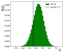
Where is the percentile of the distribution, for which the type I error is . Figure [2] shows the standard normal distribution; the shaded area represents the type I error for the percentile , which corresponds to the model exclusion condition at the level.
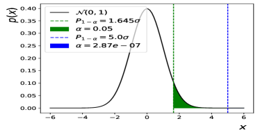
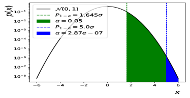
The confidence level for an observation is significantly higher. In general, the discovery threshold is set at , where the type I error is . Table [1] summarizes different confidence levels and their interpretation in high-energy physics (HEP) Lista (2016); Cranmer (2015); Cowan et al. (2011).
| Gaussian percentile | Interpretation | ||
|---|---|---|---|
| no excluded | |||
| excluded (Model exclusion) | |||
| excluded | |||
| excluded | |||
| excluded | |||
| excluded (Observation) |
2.1 Frequentist upper limit
In practical terms, the simplest approach for making estimates is to consider single-channel experiments, where we have an observed value (), an expected number of background events (), and an expected number of signal events (). Since the measurement process involves counting events in the channel, we will model it using a Poisson distribution.
For , the mean of the distribution will be , meaning that the observation is explained solely by background events. For , the mean is given by , where is known as the signal strength and measures the agreement between and the observation. In this way, to find the confidence level of both hypotheses with respect to the observation, we use the cumulative Poisson distribution, which is given by:
| (3) |
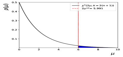
Where for and for . This cumulative distribution has a direct relation with the cumulative distribution, with degrees of freedom and (see Appendix 11). Therefore, the confidence level is given by Lista (2016):
| (4) |
The signal strength allows us to statistically assess the degree of agreement between the alternative hypothesis and the observation. In general, we can find the upper limit of the signal strength, i.e., the point at which the alternative hypothesis can no longer explain the observation. This means excluding all models with at a confidence level. By inverting the relation (4), it is possible to calculate the upper limit for all new theories, given the observation , an expected number of background events , and new physics events . Thus, we obtain:
| (5) |
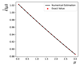
Where is the upper limit at CL, normalized to the number of signal events. For a channel with no event observation, where , the upper limit for a new model is at CL. This means that all physical theories predicting more than 3 events in that channel are excluded 111Source code. Figure [3] shows the distribution, where the shaded area represents the statistical significance , with a value of .
In the general case, when the number of observations is different from 0, the upper bounds of the model are determined by varying both the observations and the expected background Lista (2016); Cranmer (2015). Figure [4] illustrates the behavior of the upper bound for a given , as a function of the expected nuisance level 222Source code.
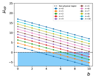
It is important to note that as the number of observations decreases, the upper bound value as a function of the background component tends to negative values. A value of implies the exclusion of the null hypothesis in the absence of signal events . This scenario presents a contradiction, as it represents a non-physical condition known as the coverage problem of the statistical estimator. To address this issue, variants of the frequentist method have been proposed that correct the coverage problem while adhering to solid probabilistic principles. These approaches include Bayesian methods and a modified version of the frequentist method Lista (2016); Cranmer (2015); Conway et al. (2005).
2.2 Bayesian upper limits
Since the upper limits obtained through the frequentist approach can lead to non-physical statistical boundaries, alternative approaches can improve the results. One of the most promising strategies is based on Bayes’ theorem:
| (6) |
Where represents the probability that the hypothesis parameterized by is true given the set of observations , and is known as the posterior distribution. , known as the likelihood function, describes the probability of observing given that the hypothesis parameterized by is true. On the other hand, is the prior distribution, which reflects the probability that the hypothesis is true before the observations are made, and is the total probability of observing across all hypotheses. In optimization processes, this latter distribution is considered a normalization factor for the posterior distribution Wang et al. (2023). From a parameter estimation perspective, sampling from the posterior distribution generally requires robust methods, such as the Metropolis-Hastings algorithm Chib and Greenberg (1995).
By incorporating an appropriate prior distribution, such as one with a minimum at , the coverage problem present in the frequentist approach is corrected. This implies that, for no value of the parameter of interest , is the null hypothesis excluded. An unbiased distribution is given by:
| (7) |
The value of is chosen to obtain p-values consistent with the critical region (i.e., ). However, the degree of subjectivity in selecting the prior distribution introduces ambiguity in the calculation of credible confidence intervals, as well as in the upper limits. In general, it has been observed that Bayesian parameter estimation leads to less restrictive upper limits, which are dependent on the choice of the prior distribution. This characteristic has limited the use of Bayesian upper limits in physics analyses with real observations Collaboration et al. (2012b, a).
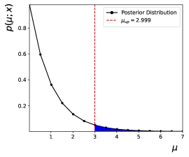
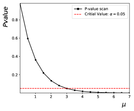
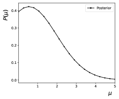
Returning to the simplified model with no observation, , and , the Bayesian upper limit for this new model is at CL. This means that, similar to the frequentist limit, all models predicting more than 3 events in this channel are excluded. Figure [5] shows the posterior distribution for the signal strength and the upper limit indicated by the red dashed line, as well as the p-value scan as a function of , with the critical value defined by the type-I error of the test 333Source Code. It is worth noting that the posterior distribution is normalized using the Gaussian quadrature technique, which offers high precision in this type of calculation when the function depends on a single parameter Golub and Welsch (1969). The normalization is defined by:
| (8) |
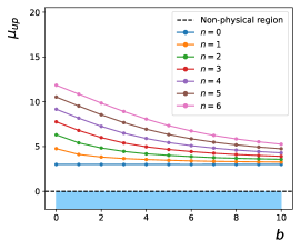
Although both methods seem to lead to the same results for the estimation of upper limits, varying the background component and the number of observed events reveals an adjustment in the upper limits that corrects the coverage issue in the estimation. Figure [6] shows the behavior of the upper limit as a function of the background component and the number of observations. Note how the null hypothesis is not excluded when the prior distribution is correctly chosen. However, manipulating the prior distribution can result in a significant shift in the upper limit value. For this reason, the Bayesian method is not widely used in the analysis of real data.
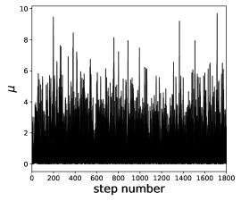
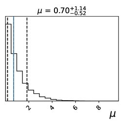
Additionally, it is possible to estimate the upper limit using the Markov Chain Monte Carlo (MCMC) technique 444Source Code. This method allows sampling from the posterior distribution based on Markov processes, as described in various sources Chib and Greenberg (1995); Raftery and Lewis (1992). In general, this approach enables the construction of the marginal posterior function for the calculation of upper limits, the estimation of standard errors (), and the necessary parameter estimation in methods such as the profile of maximum likelihood, discussed later. Figure [7] shows the sampling of the posterior distribution for the toy model, leading to an approximation of the upper limit using the percentile.
The MCMC algorithm is widely used for estimation in real multichannel experiments and incorporates systematic effects. The development of these ideas requires non-Bayesian approaches that do not depend on the choice of the prior distribution. An initial non-Bayesian approach that protects the null hypothesis is known as the modified frequentist method Read (2002); collaboration (2022a).
2.3 Modified frequentist method
In general, the construction of frequentist estimators is based on determining the confidence level associated with a statistical estimator. For a statistic , the confidence level of the hypothesis considering only the background component is given by the probability that takes a value less than or equal to the observed value Lista (2016); Barlow (2019); Read (2002).
| (9) |
where depends on the observed values: , , and . Similarly, the confidence level for the signal + background hypothesis is defined by the probability that is less than or equal to , thus:
| (10) |
The modification of the frequentist method involves the renormalization of the confidence level for the alternative hypothesis:
| (11) |
The purpose of this definition is to maintain the coverage of the estimator to protect the null hypothesis . In other words, the exclusion values of are positive. In particular, for event counting is given by:
| (12) |
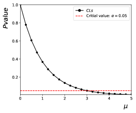
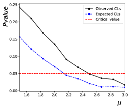
Using the expression for the cumulative Poisson distribution (Appendix 11), it is possible to find the value of for different values of the signal strength . Figure [8] shows the exploration of the p-value as a function of the signal strength for and . The upper limit is consistent with values obtained using previous methods.
In the previous sections, estimations were made for a specific point defined by , , and . Table [2] summarizes the calculation of upper limits for the three methods discussed above, evaluated for different values of and while keeping constant 555Source code.
| Observation () | Expected background () | Frequentist | Bayesian | Modified frequentist |
|---|---|---|---|---|
| 0 | 0 | 2.99 | 3.00 | 2.99 |
| 1 | 1.99 | 3.00 | 2.99 | |
| 2 | 0.99 | 3.00 | 2.99 | |
| 3 | 0.00 | 3.00 | 2.99 | |
| 1 | 0 | 4.74 | 4.76 | 4.75 |
| 1 | 3.74 | 4.11 | 4.12 | |
| 2 | 2.74 | 3.82 | 3.82 | |
| 3 | 1.74 | 3.65 | 3.65 | |
| 2 | 0 | 6.29 | 6.30 | 6.29 |
| 1 | 5.29 | 5.41 | 5.42 | |
| 2 | 4.29 | 4.83 | 4.83 | |
| 3 | 3.29 | 4.45 | 4.45 | |
The development of the concept of confidence level and the application of the Neyman-Pearson Lemma for the signal hypothesis have facilitated the creation of frequentist statistical estimators that are unbiased by prior distributions. At the LEP collider, a parameter-independent estimator was developed collaboration (2022a); Cranmer (2015). More recently, at the LHC, the estimator has been employed, which is based on the profile likelihood Lista (2016); JME (2010). This estimator maximizes the parameters for statistical and systematic uncertainty within the likelihood function to incorporate these effects in the calculation of upper limits, experimental sensitivity, or the potential observation of new physics.
2.4 Non-profile frequentist estimator
The modified frequentist method is generalized through the Neyman-Pearson Lemma, a fundamental statistical result stating that the most powerful test for hypothesis comparison is based on minimizing the Type II error. This error occurs when the null hypothesis (), which assumes only background, is not rejected despite being false. The Neyman-Pearson Lemma indicates that, given a significance level, the most efficient statistical test to discriminate between two hypotheses is based on the likelihood ratio Cranmer (2015); Lista (2016); Cowan et al. (2011).
| (13) |
The formula has an asymptotic approximation to a distribution when expressed in terms of logarithms Lista (2016). Generally, this formula is expressed as follows:
| (14) |
This expression is known as the log-likelihood ratio, and it allows for generalization to experiments with multiple channels. Consider, for example, a single-channel experiment measuring the mass of a hypothetical particle within the range of 100 to 200 GeV. Suppose the observation is , the expected number of background events is , and the model for this new particle predicts . The statistical estimator based on this distribution model is expressed as follows:
| (15) | |||||
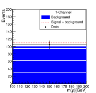
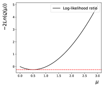
Figure [9] shows the single-channel experiment, where the error bars represent the Poisson uncertainty, , associated with the observed number of events. Additionally, it describes the behavior of the estimator as a function of the signal strength, . This reveals that the likelihood ratio defines a convex optimization problem with a unique global minimum, corresponding to the best fit of the model under the null hypothesis to describe the observation. Notably, both hypotheses can fit the observed data, making it essential to determine the set of theories that can be excluded based on the measurement of or to assess whether there is sufficient evidence to claim the discovery of the particle in question Collaboration et al. (2012b); collaboration (2022b).
The best-fit value is obtained by differentiating the log-likelihood function with respect to the parameter of interest and evaluating the result at zero. In this case, the minimum can be calculated exactly using elementary methods.
| (16) |
Estimating the best model is fundamental in current statistical estimators. In general, obtaining the best fit in experiments with multiple channels and systematic uncertainties requires advanced optimization processes and sampling techniques, which will be described later. Moreover, calculating upper limits involves sampling the distributions of the estimator under both the null and alternative hypotheses. The next section will address the sampling of the estimator and the definition of the confidence level for the signal, known as .
2.4.1 Sampling of the log-likelihood estimator
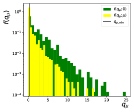
To obtain the upper limit using the estimator , the estimator can be sampled under both the null and alternative hypotheses; these distributions are labeled and , respectively. To calculate , a random number is generated following a Poisson distribution with , representing the number of observed events under the null hypothesis. Similarly, the distribution is obtained using a specific value of Lista (2016); Cranmer (2015). Figure [10] shows a schematic of the shapes of the distributions of the estimator . The value corresponds to the estimator for the observed number of events . Typically, the background-only distribution is found to the right of , while the signal + background distribution is found to the left of . The degree of agreement between the observation and the models is evaluated through the confidence level, represented by the shaded areas in the plot Cowan (2014).
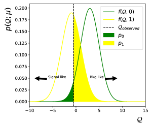
The green shaded area represents the p-value of the observation under the background-only hypothesis () and is expressed as:
| (17) |
The p-value of the null hypothesis is related to the well-known power of the test, which is the confidence level, denoted as :
| (18) |
On the other hand, the p-value for the signal + background hypothesis () is represented by the yellow shaded area, which directly corresponds to the confidence level of the hypothesis:
| (19) |
Thus, the statistical significance is a particular case of the p-value of the observation under the null hypothesis () and constitutes evidence in favor of against . Consequently, maximizing the significance is a tool for optimizing the search window. In various statistical studies, it is suggested that stronger evidence in favor of over is reflected in Lista (2016); collaboration (2022a, b):
| (20) |
This completely defines the confidence level of the signal. Using these definitions, the upper limit of the signal strength is obtained through the following strategy: 1) vary the signal strength , 2) sample the distributions and , 3) calculate the p-values corresponding to the observed estimator, and 4) determine the confidence level . In this way, the upper limit for exclusion is given by:
| (21) |
This process is typically computationally expensive due to the sampling of distributions for each value of . In the case of multiple channels and nuisance parameter estimation, parallelization is required to obtain results efficiently. This is crucial, as optimizing the search window at the phenomenological level necessitates maximizing statistical significance or other statistical metrics Flórez et al. (2016); Allahverdi et al. (2016).
In the experiment related to the invariant mass channel , we have two key estimates. The first is the expected upper limit, which is assumed under the hypothesis that the observation consists of background nuisance only. In this case, the expected upper limit is . This implies that any theory predicting more than events would be excluded, provided that events are measured. In the second case, the observed upper limit corresponds to the actual data observation. This observed upper limit is estimated as , meaning that any theory predicting more than events would be excluded based on the observation. Figure [11] shows the search for the confidence level for both the expected and observed limits 666Source code. Additionally, the distribution of the statistical estimator for is presented as an illustrative example. Finally, results obtained using the professional RooFit package, used by the CMS and ATLAS collaborations for upper limit estimation, are included Verkerke and Kirkby (2006); Schott (2012).
An important feature in this type of analysis is that when the upper limits are statistically consistent, as in this case, there is insufficient evidence to claim a discovery. In this scenario, we would accept that the null hypothesis (background-only hypothesis) adequately describes the observation. The first sign of tension between the observed data and the background-only hypothesis arises when the expected and observed upper limits differ significantly. From a statistical perspective, this discrepancy must be evaluated, and to consider the observation of a new phenomenon, the difference must exceed the threshold Lista (2016); Cranmer (2015); Collaboration et al. (2012b).
3 Experimental sensitivity using the estimator
The experimental sensitivity to detect a new physics signal depends on multiple factors, including the accelerator’s integrated luminosity, data quality, detector triggers, simulations, and accurate estimation of events associated with known physics (background) Barlow (2002). Given the vast parameter space and variety of theories, there arises a need to identify a specific search region to efficiently focus experimental efforts towards generating new discoveries Casadei (2011).
Phenomenology in high-energy physics (HEP) defines this search region as the signal region, determined by the expected number of new physics events for certain observables, such as invariant mass, transverse mass, etc. A common strategy to identify this region involves maximizing the statistical significance of observing , with events consistent with the new theory, assuming the background-only hypothesis () is true. This expected number of events is referred to as Asimov data Lista (2016); Cowan et al. (2011), and it is used to determine the parameter space window of the theory measurable in the experiment with a specific luminosity. The statistical estimator , with expected value , is given by:
| (22) |
From this value, is calculated, which allows estimating the significance in the context of a distribution corresponding to background-only hypothesis:
| (23) |
The optimal signal region for the experimental search is determined by finding the expected number of new physics events that maximizes the statistical significance. Thus:
| (24) |
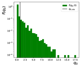
This value of is converted into units of standard deviations from a distribution. For now, this estimate assumes that the number of background events is well-determined, with no associated statistical or systematic error. Systematic effects on the background can modify both the signal region and the upper limits of theoretical predictions, and must be taken into account in phenomenological studies. Figure [12] illustrates the distribution with , which is used to estimate the significance of the new physics model with and background events. The value of is , which corresponds to standard deviations. This result can also be approximated using the estimator Flórez et al. (2016); collaboration (2022a, b):
| (25) |
This estimator is considered an approximate estimation of the signal significance and is valid when (Appendix 12). It is worth noting that this estimator has been widely used in optimizing search regions beyond the Standard Model in the context of phenomenology and experimental analysis Flórez et al. (2016); Allahverdi et al. (2016); Collaboration et al. (2012b, a).
4 Profile frequentist estimator
The estimator has been used in calculating upper limits for the mass of the Higgs boson. However, incorporating systematic effects is complex. Including these effects requires randomly varying the central values to obtain , which increases the variance and thus expands the upper limits. This phenomenon will be analyzed in detail in the section dedicated to systematic effects Barlow (2002). Currently, phenomenology and experimental analyses employ a statistical estimator, , which combines the unbiased frequentist approach with the incorporation of systematic effects through the profile likelihood. This estimator requires maximizing the likelihood function with respect to signal strength, and for single-channel experiments, it is given by Lista (2016); Cranmer (2015):
| (26) |
Where is the maximum likelihood estimator of the observation . By appropriately applying the logarithmic function, the estimator can be reformulated as a minimization problem. The hypothesis test without considering systematic effects is expressed as follows:
| (27) |
Finally, to quantify the degree of disagreement between the observation and the hypothesis, the p-value of the observation is calculated:
| (28) |
Where is the observed value of the estimator in the data, and represents the distribution of the estimator for a specific value of . Generally, this is an optimization problem to obtain the best fit of the model, followed by a sampling problem to determine . Specifically, in the case of upper limit searches, the statistical test simplifies to Lista (2016); Read (2002):
| (29) |
Where is adjusted to avoid excluding values smaller than the maximum likelihood estimator (i.e., in the non-physical case). With these definitions, the confidence level () associated with the observation under the background-only hypothesis is expressed as:
| (30) |
Therefore, the confidence level of the signal, , is defined as:
| (31) |
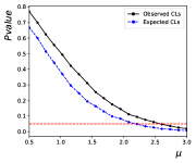
As in the case of the unprofiled estimator, the upper limit is defined by , which corresponds to the model exclusion criterion. For the single-channel experiment with , , and , a scan is performed by sampling the distribution for both hypotheses. Figure [13] shows the scan of the confidence level for the signal strength as a function of , as well as the distributions of and for 777Source code.
At each point, the maximum likelihood estimator is obtained using the specialized optimize package Virtanen et al. (2018). The expected upper limit is , and the observed upper limit is . These values are fully consistent with the upper limits obtained using the estimator .
5 Experimental sensitivity using the estimator
The statistical significance is calculated using a strategy similar to that illustrated for the estimator . First, the value is obtained using the statistical test:
| (32) |
where for signal sensitivity. The significance is obtained by finding the p-value of the possible observation using the background-only distribution :
| (33) |
In the asymptotic limit, the significance can be approximated as Lista (2016); Cowan (2014). As mentioned previously, the signal region is obtained by finding the event window that maximizes the statistical significance, Equation (24). In the single-channel case, a statistical significance of is obtained, which translates to standard deviations, consistent with the significance calculation using the estimator . Figure [14] shows the background-only distribution and the observed value in the Asimov data. The area under the distribution for positive values of represents the statistical significance of the expected new physics events Cranmer (2015).
6 Upper Limits for multi-channel experiments
In the multi-channel case, the likelihood associated with the signal strength for the complete observation is determined by the joint likelihood of all channels Wang et al. (2023):
| (34) |
Where it is assumed that the information in each channel is independently and identically distributed. The definitions of the estimators and for a single channel naturally extend to the multi-channel case using the properties of logarithms. Thus, the statistical estimators are fully defined as follows, respectively:
| (35) |
| (36) |
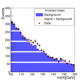
As an example, synthetic data associated with a resonance near the measured mass of the Higgs boson were simulated, with an exponential background component characteristic of the invariant mass of a diphoton system. A total of 30 channels were simulated to numerically illustrate the discovery reported by the CMS collaboration in 2012 Collaboration et al. (2012b). Figure [15] shows the resonance data with a mass similar to the measured Higgs boson mass under an exponential background component (blue shaded area). Additionally, the alternative signal + background hypothesis is shown, which could be consistent with the observation.
As in the 2012 search, several signal models with masses ranging from 100 to 160 GeV in steps of 6 GeV will be assumed. For each signal point, the expected upper limit (), representing a measurement compatible with the background-only hypothesis, and the observed upper limit using the synthetic data will be calculated. Given the data observation, the upper limits allow for excluding the Higgs model at a specific mass or rejecting the background-only hypothesis in favor of the model with this new particle. Typically, this discrepancy is indicated by the difference between the expected and observed upper limits; when this difference is large, it must be quantified in terms of the criterion to report a discovery Lista (2016).
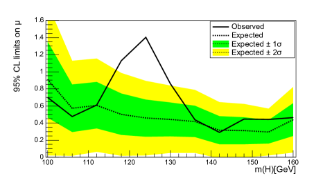
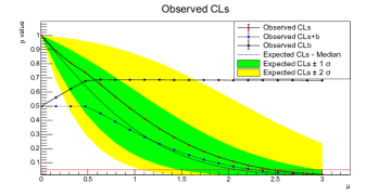
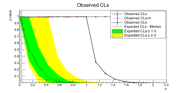
Figure [16] shows the upper limit values as a function of the hypothetical particle mass using the estimator . The error bands at and are calculated using Wald’s asymptotic approximation Conway et al. (2005). Note that low- and high-mass models are excluded at a confidence level, while for there is a discrepancy between upper limits. In HEP, this indicates that the observation significantly deviates from the background-only hypothesis. This discrepancy allows for reporting a discovery if it surpasses the criterion; otherwise, it is considered merely as evidence of a potential unknown process 888Source code.
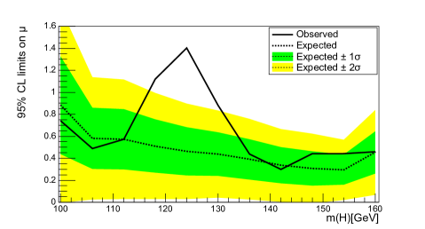
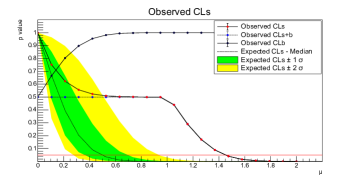
On the other hand, Figure [17] shows the upper limit values as a function of the hypothetical particle mass using the estimator. In the generation of each random experiment, is found using the Scipy.optimize package. The error bands at and are estimated using Wald’s asymptotic approximation . Note the consistency of the results using both estimators. The primary difference lies in the approach to incorporating systematic uncertainties in the estimation of upper limits, significance, and tension, which is why the profile likelihood is currently used by the CMS and ATLAS collaborations for these estimations Collaboration et al. (2012b, a). Finally, to estimate the discrepancy between the observation and the expected number of events, the p-value of the observation is calculated under the assumption that the background-only hypothesis is correct.
| (37) |
where is the number of observed events.
| (38) |
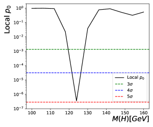
Figure [18] shows the local p-value as a function of the particle mass. The dashed lines indicate the evidence region and the discovery region. This graph illustrates the statistical behavior of the p-value in the search for the Higgs boson in 2012 Collaboration et al. (2012b).
7 Upper Limits including systematic uncertainties, Bayesian approach
The inclusion of systematic effects in the calculation of upper limits, experimental sensitivity, and observation requires a Bayesian approach. This strategy extends the likelihood function by including typically Gaussian distributions to model effects such as efficiency, luminosity, Monte Carlo event estimation, and others Lista (2016); Cranmer (2015); Junk (1999). In particular, to establish the reconstruction efficiency of background events, a nuisance parameter () centered on the expected value of can be included. Thus, the parameter of the Poisson distribution is defined by:
| (39) |
where the efficiency follows a binomial distribution . The standard deviation of the likelihood adjusts the uncertainty of the number of background events across the observable spectrum, typically ranging from 5 to 20% in analyses Collaboration et al. (2012b); Flórez et al. (2016). Thus, the extended likelihood function is given by:
| (40) |
The non-informative prior distribution naturally extends to:
| (41) |
Using Bayes’ theorem, the posterior distribution is obtained.
| (42) |
This means that to establish the upper limits of or the experimental sensitivity, the posterior must be marginalized to find the profile . This is a standard probability calculation and requires numerical integration or sampling of the posterior distribution using, for example, the Markov Chain Monte Carlo (MCMC) algorithm Raftery and Lewis (1992); Wang et al. (2023). In any case, the probability profile is given by:
| (43) |
The marginalization process correctly propagates the effect of systematic uncertainty in the upper limits. In general, the correlation shifts the limit values to higher values, thereby restricting the sensitivity of a model in the experiment or the exclusion power in an experimental study Conway et al. (2005). As mentioned previously, the expected and observed upper limits are defined over the marginal distribution:
| (44) |
Figure [19] shows the posterior distribution as a function of the signal strength and the efficiency in estimating background events (), for the channel with , , , and a systematic uncertainty of for the background events 999Source code. Similarly, Figure [20] shows the marginal distribution obtained using the double Gaussian quadrature method Golub and Welsch (1969).
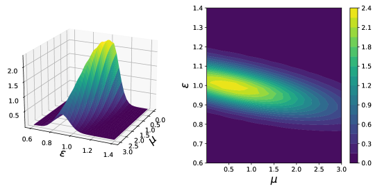
By varying the systematic uncertainty, it is possible to find the observed upper limits and the correlation effect between parameters. Table [3] shows the behavior of the observed upper limit as a function of for the numerical approximation (Gaussian quadrature) and for the sampling generated by the Metropolis algorithm, as well as the correlation coefficient indicating how uncertainty limits the exclusion power of the model. It is important to note that for high-dimensional posterior distributions, there are no quadrature rules that allow for accurately estimating the marginal distribution. In such cases, the Metropolis algorithms and optimization methods have been widely applied Collaboration et al. (2012a, b).
| Gaussian quadrature | MCMC algorithm | Correlation coef | |
|---|---|---|---|
| 0.05 | 2.80 | 2.71 | -0.32 |
| 0.10 | 3.34 | 3.31 | -0.54 |
| 0.15 | 4.09 | 4.13 | -0.68 |
| 0.20 | 4.91 | 4.66 | -0.77 |
| 0.25 | 5.79 | 5.80 | -0.88 |
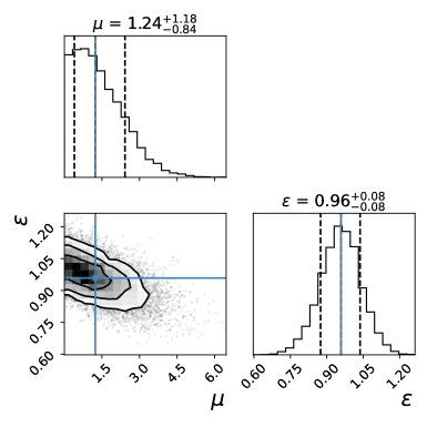
In particular, the emcee package was used for sampling the extended posterior distribution shown above Foreman-Mackey et al. (2013); Bocklund et al. (2019). Figure [21] shows the corner plot of the posterior distribution along with the marginal distributions associated with the signal strength and the reconstruction efficiency 101010Source code. Additionally, the maximum likelihood estimators of the posterior are shown; these parameters are required for the profile likelihood method presented in the following section.
8 Upper Limits using the profile binned likelihood
The profile binned likelihood method is chosen by particle physics collaborations to present phenomenology studies and experimental analyses. As shown above, this method is based on estimating the signal confidence level through a fully frequentist approach focused on parameter estimation Lista (2016); Barlow (2002). To include systematic effects, the likelihood function is extended with appropriate distribution functions to describe efficiency effects with a given width . This methodology requires maximizing the likelihood function and obtaining the background profile as a function of the signal strength . The improvement lies in replacing the normalization of the posterior distribution with a multivariable optimization problem, which is computationally less costly and leads to limits that allow for better model exclusion. The statistical estimator is given by Conway et al. (2005); Collaboration et al. (2012b, a):
| (45) |
where and are the unconditional maximum likelihood estimators, and is the conditional maximum likelihood estimator. Frequentist limits are generally less restrictive and allow for exploring regions of significance while adequately accounting for systematic effects. Similar to the Bayesian approach, maximizing the likelihood as a function of enables finding the profile likelihood that propagates the effect of the background parameters .
Systematic effects lead to higher upper limits, which restrict the model exclusion power and experimental sensitivity. For example, in a single-channel experiment with , , and , the optimize package is used to find the best-fit parameters, and Monte Carlo methods are applied to sample the estimator . The extended likelihood function is given by:
| (46) |
where maximizing the likelihood function for the efficiency yields the conditional nuisance estimator :
| (47) |
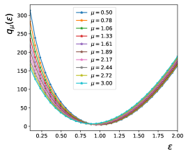
For the single-channel experiment, Figure [22] shows the profile of the nuisance parameter for various values of . The maximum value of the likelihood function shifts depending on the signal strength 111111Source code. The right plot shows the maximum likelihood estimate using both Equation (47) and the optimization package. This result indicates the maximal behavior of the uncertainty for each value of the signal strength , ensuring model exclusion as restrictive as allowed by the uncertainty . More generally, the multi-channel case requires a fully numerical procedure to find the profiles of the nuisance parameters and Lista (2016); Cranmer (2015).
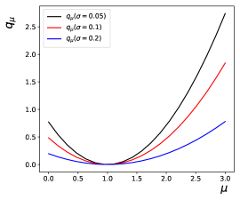
To illustrate the behavior of the estimator as a function of the systematic uncertainty , a sweep over the signal strength is performed while optimizing the estimator for the current values of the observation, background component, and signal events. Figure [23] shows the profile binned likelihood for the single-channel experiment as a function of the width of the systematic uncertainty. A larger uncertainty leads to a higher upper limit, which can be quantified using Wald’s approximation Cowan et al. (2011).
The green dashed line represents the observed upper limit for each profile likelihood. For example, for , the observed upper limit is , which contrasts with the value obtained from the Bayesian approach (Table [3], ), a smaller value. The right plot represents the search for the p-value while fixing the value of the systematic uncertainty. Obtaining the pseudo-data requires generating an observation consistent with the background-only hypothesis with , and for the signal + background hypothesis with in each observable channel. For each generated value of across all channels, the optimization of is performed.
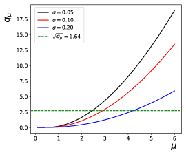
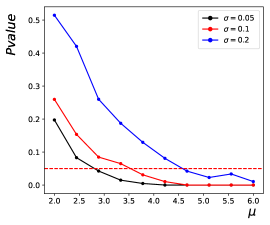
Table [4] shows the upper limit values using the grouped profile likelihood method for several values of . In comparison with the upper limits obtained by the Bayesian method, consistency is observed within the statistical confidence levels inherent to the sampling.
| Profile likelihood Ratio | MCMC algorithm | |
|---|---|---|
| 0.05 | 2.80 | 2.71 |
| 0.10 | 3.52 | 3.31 |
| 0.20 | 4.57 | 4.66 |
For the multi-channel case, results are very close between the upper limits without uncertainty and those found using the profile likelihood method. This behavior is attributed to the combined uncertainty of the background across the 30 channels, which does not significantly affect the confidence in the signal strength, especially in the resonance region collaboration (2022a); Collaboration et al. (2012a); Cowan et al. (2011). Table [5] shows the upper limit values for several mass points and uncertainty .
| Mass()[GeV] | Method: Profile likelihood ratio | |
|---|---|---|
| 110 | 0.1 | 0.43 |
| 110 | 0.2 | 0.45 |
| 124 | 0.1 | 1.45 |
| 124 | 0.2 | 1.46 |
| 142 | 0.1 | 0.29 |
| 142 | 0.2 | 0.31 |
8.1 Experimental sensitivity with systematic effects
In the case of determining the experimental sensitivity for a specific model , the Asimov data are used, and a modification is applied to the statistical estimator Lista (2016).
| (48) |
In the Wald approximation, the significance is approximately given by:
| (49) |
Figure [24] shows the profile likelihood for various values of the systematic uncertainty . It demonstrates how statistical significance is impacted by uncertainty. In general, greater uncertainty in the estimation of background events leads to a loss of sensitivity in a potential experimental analysis aiming to validate a new hypothetical model.
There are alternative methods to establish statistical significance Cowan et al. (2011), such as:
| (50) |
However, in general, experimental sensitivity is overestimated because the maximal information of is not fully captured in the profile likelihood. Table [6] shows the statistical significance for various values of systematic uncertainty . This effect reduces experimental sensitivity and should be calculated using the profile binned likelihood method. Note that the approximation is no longer valid due to the convolution effect of counting and efficiency distributions.
| 0.05 | 0.878 | 0.932 | 0.931 |
| 0.1 | 0.695 | 0.932 | 0.912 |
| 0.2 | 0.443 | 0.932 | 0.877 |
As shown in Table [6], when there is a 20% uncertainty in the background component, the sensitivity is overestimated by nearly a factor of two. Furthermore, if the effects of luminosity and signal Monte Carlo efficiency are included, the significance becomes misestimated. All these effects should be taken into account in phenomenological studies to consider potential experimental and simulation impacts in the search for new physics Barlow (2002).
9 Upper Limits with RooFit
Due to the computational complexity of calculating upper limits and experimental sensitivity, high-level statistical packages have been developed for the accurate definition of distribution functions, integration methods, and Monte Carlo generation. Among these, RooFit, developed by Stanford University, stands out for its application in the CMS and ATLAS collaborations Verkerke and Kirkby (2006); Schott (2012). Extensive documentation of these implementations can be found in the RooFit Workbook. This document provides access to the creation of the RooFit workspace, as well as the code to obtain upper limits using the profile binned likelihood method and the asymptotic approximation 121212Source code. The asymptotic approximation is widely discussed in other sources Cowan (2014); Cowan et al. (2011), so the conceptual part was omitted in this report. Figure [25] shows the upper limits for the mass point using the profile likelihood method and the asymptotic approximation. Note the agreement in the values of both methods, demonstrating a significant discrepancy between observation and the background-only hypothesis 131313Source code.
10 Discussion
The findings of this study underscore the fundamental importance of statistical inference methods in particle physics, not only for validating experimental results but also for setting precise exclusion limits that enhance our understanding of physical models. The implementation of the proposed code provides a robust framework for conducting rapid computations, a critical requirement for real-time data analysis in high-stakes experiments like those conducted at the LHC. These computational tools empower researchers to swiftly assess the significance of potential new models, supporting confident hypothesis exclusion and, ultimately, the announcement of discoveries.
A notable strength of this study is the combined use of frequentist and Bayesian approaches, which enables adaptability across various experimental scenarios and enhances the accuracy of results in the presence of systematic uncertainties. This dual approach ensures that researchers can effectively manage complex collider data, addressing both expected behaviors and unexpected fluctuations with statistical rigor.
Moreover, by making the source code publicly available, this work provides a valuable resource for the scientific community, allowing researchers to perform similar calculations on models of their interest. This accessibility fosters reproducibility and further innovation, supporting the exploration of physics beyond the Standard Model. Future developments could focus on optimizing the computational efficiency of these methods and integrating machine learning techniques to enhance model evaluation in multi-dimensional parameter spaces, thereby expanding the applicability of these tools to even more challenging experimental conditions.
In summary, the methodologies and tools presented here offer a comprehensive resource for high-energy physics research, serving both as a practical aid for immediate analysis and as a foundation for advancing the field toward new discoveries.
References
- Read [2002] Alexander L Read. Presentation of search results: the cls technique. Journal of Physics G: Nuclear and Particle Physics, 28(10):2693, 2002.
- Cowan [2014] Glen Cowan. Statistics for searches at the lhc. In LHC Phenomenology, pages 321–355. Springer, 2014.
- Feldman and Cousins [1998] Gary J Feldman and Robert D Cousins. Unified approach to the classical statistical analysis of small signals. Physical review D, 57(7):3873, 1998.
- Lista [2016] Luca Lista. Practical statistics for particle physicists. arXiv preprint arXiv:1609.04150, 2016.
- Cranmer [2015] Kyle Cranmer. Practical statistics for the lhc. arXiv preprint arXiv:1503.07622, 2015.
- Barlow [2019] Roger John Barlow. Practical statistics for particle physics. arXiv preprint arXiv:1905.12362, 2019.
- Verkerke and Kirkby [2006] Wouter Verkerke and David Kirkby. The roofit toolkit for data modeling. In Statistical Problems in Particle Physics, Astrophysics and Cosmology, pages 186–189. World Scientific, 2006.
- Schott [2012] Grégory Schott. Roostats for searches. arXiv preprint arXiv:1203.1547, 2012.
- Conway et al. [2005] John Conway, CDF Collaboration, et al. Calculation of cross section upper limits combining channels incorporating correlated and uncorrelated systematic uncertainties. Collider Detector at Fermilab collaboration note, 6428, 2005.
- Casadei [2011] Diego Casadei. Statistical methods used in atlas for exclusion and discovery. arXiv preprint arXiv:1108.2288, 2011.
- JME [2010] CMSPAS JME. Cms physics analysis summary. CMS - internal note, 2010.
- Junk [1999] Thomas Junk. Confidence level computation for combining searches with small statistics. Nuclear Instruments and Methods in Physics Research Section A: Accelerators, Spectrometers, Detectors and Associated Equipment, 434(2-3):435–443, 1999.
- Barlow [2002] Roger Barlow. Systematic errors: facts and fictions. arXiv preprint hep-ex/0207026, 2002.
- Collaboration et al. [2012a] Atlas Collaboration et al. Observation of a new particle in the search for the standard model higgs boson with the atlas detector at the lhc. arXiv preprint arXiv:1207.7214, 2012a.
- Sinervo [2002] Pekka K Sinervo. Signal significance in particle physics. arXiv preprint hep-ex/0208005, 2002.
- Cowan et al. [2011] Glen Cowan, Kyle Cranmer, Eilam Gross, and Ofer Vitells. Asymptotic formulae for likelihood-based tests of new physics. The European Physical Journal C, 71:1–19, 2011.
- Flórez et al. [2016] Andrés Flórez, Luis Bravo, Alfredo Gurrola, Carlos Ávila, Manuel Segura, Paul Sheldon, and Will Johns. Probing the stau-neutralino coannihilation region at the lhc with a soft tau lepton and a jet from initial state radiation. Physical Review D, 94(7):073007, 2016.
- Wang et al. [2023] Xilu Wang, Yaochu Jin, Sebastian Schmitt, and Markus Olhofer. Recent advances in bayesian optimization. ACM Computing Surveys, 55(13s):1–36, 2023.
- Chib and Greenberg [1995] Siddhartha Chib and Edward Greenberg. Understanding the metropolis-hastings algorithm. The american statistician, 49(4):327–335, 1995.
- Collaboration et al. [2012b] Cms Collaboration et al. Observation of a new boson at a mass of 125 gev with the cms experiment at the lhc. arXiv preprint arXiv:1207.7235, 2012b.
- Golub and Welsch [1969] Gene H Golub and John H Welsch. Calculation of gauss quadrature rules. Mathematics of computation, 23(106):221–230, 1969.
- Raftery and Lewis [1992] Adrian E Raftery and Steven M Lewis. [practical markov chain monte carlo]: comment: one long run with diagnostics: implementation strategies for markov chain monte carlo. Statistical science, 7(4):493–497, 1992.
- collaboration [2022a] CMS collaboration. A portrait of the higgs boson by the cms experiment ten years after the discovery. Nature, 607(7917):60–68, 2022a.
- collaboration [2022b] ATLAS collaboration. A detailed map of higgs boson interactions by the atlas experiment ten years after the discovery. Nature, 607(7917):52–59, 2022b.
- Allahverdi et al. [2016] Rouzbeh Allahverdi, Mykhailo Dalchenko, Bhaskar Dutta, Andrés Flórez, Yu Gao, Teruki Kamon, Nikolay Kolev, Ryan Mueller, and Manuel Segura. Distinguishing standard model extensions using monotop chirality at the lhc. Journal of High Energy Physics, 2016(12):1–13, 2016.
- Virtanen et al. [2018] Pauli Virtanen, Ralf Gommers, Evgeni Burovski, Travis E Oliphant, David Cournapeau, Warren Weckesser, Pearu Peterson, Stefan van der Walt, Josh Wilson, Nikolay Mayorov, et al. Scipy/scipy: Scipy 1.1. 0. Zenodo, 2018.
- Foreman-Mackey et al. [2013] Daniel Foreman-Mackey, David W Hogg, Dustin Lang, and Jonathan Goodman. emcee: the mcmc hammer. Publications of the Astronomical Society of the Pacific, 125(925):306, 2013.
- Bocklund et al. [2019] Brandon Bocklund, Richard Otis, Aleksei Egorov, Abdulmonem Obaied, Irina Roslyakova, and Zi-Kui Liu. ESPEI for efficient thermodynamic database development, modification, and uncertainty quantification: application to Cu–Mg. MRS Communications, pages 1–10, jun 2019. ISSN 2159-6859. doi:10.1557/mrc.2019.59.
11 Appendix A: Poisson cumulative distribution
The confidence level associated with a specific signal strength is determined by the cumulative distribution function (CDF). There is a relation that links the CDF of the Poisson distribution to that of the distribution. By applying the definition of the confidence level, we obtain:
| (51) |
By applying integration by parts, where , , , and , we obtained the following result:
| (52) |
By once again applying integration by parts, with , , , and , the following expression is obtained:
| (53) |
Finally, by integrating once more by parts, with , , , and , we obtain:
| (54) |
| (55) |
At this stage, a pattern can be discerned in the results obtained after repeatedly applying integration by parts. Specifically, the evaluation of the integral as equal zero, while for , a term of the following form is obtained:
| (56) |
Thus, after performing integration by parts, the following result is obtained:
| (57) |
| (58) |
| (59) |
This result corresponds to the cumulative distribution function (CDF) of the Poisson distribution. This distribution would then be related to the cumulative distribution () as follows:
| (60) |
12 Appendix B: Statistical significance for small values of signal
There are two approaches to assess the significance of a potential new physics signal: using the estimator or through the test statistic . In the first approach, a Gaussian approximation is obtained by evaluating the statistical estimator at its central values.
| (61) |
By defining , we can calculate the expected value for the distributions of kackground only () and signal + background (), respectively.
| (62) |
In this way, we can quantify the number of standard deviations between the expected number of background events and signal + background events across all channels.
| (63) | |||||
Where the standard error of the distribution is calculated as:
| (64) | |||||
With , which follows a Poisson distribution. Similarly, the number of standard deviations for the signal + background distribution is:
| (65) | |||||
The standard error of the distribution is calculated in a similar way:
| (66) |
On the other hand, in the second scenario, the test statistic , in the context of single-channel counting experiments, is defined from the Poisson likelihood function:
| (67) |
The profile likelihood for the null hypothesis is given by:
| (68) |
In this case, the maximum likelihood parameter is . Using the Asimov data, where , and Wilks’ approximation Conway et al. [2005], we have:
| (69) |
Finally, by expanding the logarithmic function under the condition , we obtain the Gaussian approximation of the significance:
| (70) |