ReMatching Dynamic Reconstruction Flow

Abstract

Reconstructing dynamic scenes from image inputs is a fundamental computer vision task with many downstream applications. Despite recent advancements, existing approaches still struggle to achieve high-quality reconstructions from unseen viewpoints and timestamps. This work introduces the ReMatching framework, designed to improve generalization quality by incorporating deformation priors into dynamic reconstruction models. Our approach advocates for velocity-field-based priors, for which we suggest a matching procedure that can seamlessly supplement existing dynamic reconstruction pipelines. The framework is highly adaptable and can be applied to various dynamic representations. Moreover, it supports integrating multiple types of model priors and enables combining simpler ones to create more complex classes. Our evaluations on popular benchmarks involving both synthetic and real-world dynamic scenes demonstrate a clear improvement in reconstruction accuracy of current state-of-the-art models.

1 Introduction

This work addresses the challenging task of novel-view dynamic reconstruction. That is, given a set of images of a dynamic scene evolving over time, the task objective is to render images from any novel view or intermediate point in time. Despite significant progress in dynamic reconstruction (Lombardi et al., 2021; Fridovich-Keil et al., 2023; Yunus et al., 2024), effectively learning dynamic scenes still remains an open challenge. The main hurdle arises from the typically sparse nature of multi-view inputs, both temporally and spatially. While tackling sparsity often involves incorporating some form of prior knowledge into the dynamic reconstruction model - either from a physical prior such as rigidity (Sorkine & Alexa, 2007), or learnable priors derived from large foundation models (Ling et al., 2024; Wang et al., 2024) - the optimal scheme for integrating these priors without compromising the fidelity of model reconstructions remains unclear.

To address this issue, this paper presents the ReMatching framework, a novel approach for designing and integrating deformation priors into dynamic reconstruction models. The ReMatching framework has three core goals: i) suggest an optimization objective that aims at achieving a reconstruction solution that is closest to satisfying the prior regularization; ii) ensure applicability to various model functions, including time-dependent rendered pixels or particles representing scene geometry; and, iii) provide a flexible design of deformation prior classes, allowing more complex classes to be built from simpler ones.

To support the usage of rich deformation prior classes, we advocate for priors expressed through velocity fields. A velocity field is a mathematical object that describes the instantaneous change in time the deformation induces. As such, a velocity field can potentially provide a simpler characterization of the underlying flow deformation. For example, the complex class of volume-preserving flow deformations is characterized by the condition of being generated by divergence-free velocity fields (Eisenberger et al., 2019). However, representing a deformation through its generating velocity field typically necessitates numerical simulation for integration, leading to training instability and expressivity challenges. Nevertheless, recent progress in flow-based generative models (Ben-Hamu et al., 2022; Lipman et al., 2022; Albergo et al., 2023) supports simulation-free flow training, inspiring this work to explore simulation-free training for flow-based dynamic reconstruction models. Therefore, our framework is specifically designed to integrate with dynamic reconstruction models that represent dynamic scenes directly through time-dependent reconstruction functions (Pumarola et al., 2021; Yang et al., 2023).

Exploiting the simplicity offered by velocity-field-based deformation prior classes, we observe that the projection of a time-dependent reconstruction function onto a velocity-field prior class can be framed as a flow-matching problem, solvable analytically. The opportunity to access the projected flow is reminiscent of the Alternating Projections Method (APM) (Deutsch, 1992), a greedy algorithm guaranteed in finding the closest points between two sets. Therefore, we suggest an optimization objective aimed at re-projecting back onto the set of reconstruction flows. This corresponds to a flow-matching loss that we term the ReMatching loss. Our hypothesis is that by mimicking the APM, this optimization would converge to solutions that not only meet the reconstruction objective, but also reach the closest possible alignment to the required prior class. By doing so, we achieve the desired goal of improving generalization without compromising solutions’ fidelity levels.

We instantiate our framework with a dynamic model based on the popular Gaussian Splats (Kerbl et al., 2023) rendering model. We explore several constructions for deformation prior classes including piece-wise rigid and volume-preserving deformations. Additionally, we demonstrate our framework’s usability for two different types of time-dependent functions: rendered image intensity values, and particle positions representing scene geometry. Lastly, we evaluate our framework on standard dynamic reconstruction benchmarks, involving both synthetic and real-world scenes, and showcase clear improvement in generalization quality.

2 Related Work

Flow-based 3D dynamics.

There is an extensive body of works utilizing flow-based deformations for 3D related problems. For shape interpolation, (Eisenberger et al., 2019) considers volume-preserving flows. For dynamic geometry reconstruction, (Niemeyer et al., 2019) suggests learning neural parametrizations of velocity fields. This representation is further improved by augmenting it with a canonicalized object space parameterization (Rempe et al., 2020) or by simultaneously optimizing for 3D reconstruction and motion flow estimation (Vu et al., 2022). Similarly to (Niemeyer et al., 2019), (Du et al., 2021) suggests flow-based representation of dynamic rendering model based on a neural radiance field (Mildenhall et al., 2020). More recently, (Chu et al., 2022; Yu et al., 2023) explores combining a time-aware neural radiance field with a velocity field for modelling fluid dynamics. In contrast to our framework they focus exclusively on recovering the deformation of specific fluids i.e. smoke and not on reconstructing generic non-rigid objects.

Dynamic novel-view rendering models.

Neural Radiance Fields (NeRF) (Mildenhall et al., 2020) is a popular image rendering model combining an implicit neural network with volumetric rendering. Several follow-up works (Pumarola et al., 2021; Park et al., 2021a; Tretschk et al., 2021) explore using NeRF for non-rigid reconstruction, by optimizing for time-dependent deformations. More recently, several works (Fridovich-Keil et al., 2023; Cao & Johnson, 2023; Wu et al., 2023; Song et al., 2023; Guo et al., 2023) try to address the training and inference inefficiencies of continuous volumetric representations by incorporating planes and grids into a spatio-temporal NeRF. An alternative to NeRF, suggesting an explicit scene representation, is the Gaussian Splatting (Kerbl et al., 2023) rendering model. Several works incorporate dynamics with Gaussian Splatting. (Yang et al., 2023) introduce a time-conditioned local deformation network. Similarly, (Wu et al., 2023) also relies on a canonical representation of a scene but further improves efficiency by considering a deformation model based on on $k$-planes (Fridovich-Keil et al., 2023). (Lu et al., 2024) propose the integration of a global deformation model.

3 Method

Given a collection of multi-view images, $\displaystyle F_{t}=\left\{I_{i}^{t}\right\}_{i=1}^{M}$, captured at $T$ time steps, from $M$ viewing directions, we seek to develop an image-based model for novel-view synthesis that can effectively render new images from unseen viewpoints in any direction ${\bm{d}}\in\mathcal{S}^{2}$ and any time $t\in\left[t_{1},t_{T}\right]$. Since we aim to support several time-dependent elements in a dynamic reconstruction model, we employ a general notation for a dynamic image model. That is,

$$t\mapsto\Psi_{t}=\left\{\psi(t)\,|\,\psi:\mathbb{R}_{+}\rightarrow V\right\},$$ (1)

with $\Psi_{t}$ representing the evaluation at time $t$ of all of the model components. Each element function $\psi:\mathbb{R}_{+}\rightarrow V$, where $V$ is a vector space, can specify any time-dependent quantity specified by the model. $V$ denotes a different vector space depending on the definition of $\psi$. For instance, if $\psi$ models time-dependent image intensity values, $V=C^{1}(\mathbb{R}^{d})=\left\{f|f:\mathbb{R}^{d}\rightarrow\mathbb{R},\nabla{f}\textrm{ exists and continuous}\right\}$ with $d=2$. Whereas, if $\psi$ models the time-dependent position of $n$ particles representing the underlying scene geometry, $V=\mathbb{R}^{n\times d}$ with $d=3$. Lastly, in what follows, we interchangeably switch between the notations $\psi(t)$ and $\psi_{t}$.

We defer the specific details of the time-dependent reconstruction function $\Psi_{t}$ to Section 5 and begin by describing our proposed framework for incorporating priors via velocity fields.

3.1 Velocity fields

We consider a velocity field to be a time-dependent function of the form:

$$v:\mathbb{R}^{d}\times\mathbb{R}_{+}\rightarrow\mathbb{R}^{d},$$ (2)

where usually $d=3$ or $d=2$. A velocity field defines a time-dependent deformation in space $\phi_{t}:\mathbb{R}^{d}\rightarrow\mathbb{R}^{d}$, also known as a flow, via an Ordinary Differential Equation (ODE):

$$\begin{dcases}\frac{\partial}{\partial t}\phi_{t}({\bm{x}})=v(\phi_{t}({\bm{x}}),t)\\ \phi_{0}({\bm{x}})={\bm{x}}.\end{dcases}$$ (3)

Flow-based deformations are an ubiquitous modeling tool (Rezende & Mohamed, 2015; Chen et al., 2018) that has been extensively used in various dynamic reconstruction tasks (Niemeyer et al., 2019; Du et al., 2021). In a dynamic reconstruction model, a flow deformation can be incorporated by defining a time-dependent function $\psi_{t}:\mathbb{R}^{d}\rightarrow\mathbb{R}$ as a push-forward of some reference function $\psi_{0}$, i.e., $\psi_{t}=\phi_{t*}\psi_{0}$. One key advantage of flow-based deformations is that they enable simple parametrizations for the velocity field, in turn facilitating the integration of priors into the model. For example, restricting $\phi_{t}$ to be volume-preserving can be achieved by imposing the condition $\operatorname{div}(v)=0$ (Eisenberger et al., 2019).

However, recovering $\psi_{t}$ values in the case $\psi_{t}=\phi_{t*}\psi_{0}$ is not explicit. Typically, this is achieved by solving the continuity equation

$$\frac{\partial}{\partial{t}}\psi_{t}({\bm{x}})+\operatorname{div}{\left(\psi_{t}({\bm{x}})v_{t}\left({\bm{x}}\right)\right)}=0,\forall{\bm{x}}\in\mathbb{R}^{d},$$ (4)

which necessitates a numerical simulation. This introduces challenges for training flow-based models, as errors in the numerical simulation can destabilize the optimization process. Therefore, to overcome this hurdle, our framework assumes a reconstruction model consisting of functions $\psi_{t}$ that are simulation-free, i.e., each evaluation of $\psi_{t}$ requires only a single step. Coupling $\psi_{t}$ to a prior class stemming from velocity-field-based formulation is the core issue our framework aims to address, described in the following section.

3.2 Flow ReMatching

We assume that for a time-dependent reconstruction function, $\psi_{t}\in\Psi_{t}$, there exists an underlying flow $\phi_{t}$ such that $\psi_{t}$ can be described as a push-forward by $\phi_{t}$. We refer to such $\phi_{t}$ as reconstruction flow and denote its velocity field by $v_{t}$. Under our assumption that $\psi_{t}$ is simulation-free, neither $\phi_{t}$ nor $v_{t}$ is directly accessible. Nevertheless, let us assume that we can work with an element $v_{t}\in\mathcal{V}$, where $\mathcal{V}$ represents the set of all the possible reconstruction generating velocity fields. Let $\mathcal{P}\subset\left\{u_{t}\,|\,u:\mathbb{R}^{d}\times R_{+}\rightarrow\mathbb{R}^{d}\right\}$ be a prior class of velocity fields to which $v$ should belong. In Section 4, we discuss different choices for a class $\mathcal{P}$.

In some of the choices for $\mathcal{P}$, requiring $v\in\mathcal{P}$ could be over-restrictive, conflicting with the fact that $v$ also adheres to generate the reconstruction flow. Hence, an appealing objective would be to optimize $v$ so that it is the closest element to $\mathcal{P}$ out of the set $\mathcal{V}$. We suggest an optimization procedure mimicking the alternating projections method (APM) (Deutsch, 1992). The APM is an iterative procedure where alternating orthogonal projections are performed between two closed Hilbert sub-spaces $V$ and $P$. Specifically, $v_{k+1}=\operatorname{proj}_{V}\left(\operatorname{proj}_{P}(v_{k})\right)$ guarantees the convergence of $v_{k}$ to $\mathrm{dist}(V,P)$. Following this concept, our next step is to find a suitable notion for defining the projection operator for reconstruction generating velocity fields.

Since $v$ is unknown, in our case, we utilize the continuity equation (4), which provides both a sufficient and a necessary condition for the generating velocity field of $\phi_{t}$ in terms of $\psi_{t}$ and its partial derivatives. In particular, we propose a projection procedure corresponding to the following matching optimization problem on the reconstruction flow:

$$u(\cdot,t)=\operatorname*{arg\,min}_{u_{t}\in\mathcal{P}}\rho(u_{t},\psi_{t}),$$ (5)

where,

$$\rho(u_{t},\psi_{t})=\int\left|\frac{\partial}{\partial{t}}\psi_{t}({\bm{x}})+\operatorname{div}{\left(\psi_{t}({\bm{x}})u_{t}({\bm{x}})\right)}\right|^{2}\,d{\bm{x}}.$$ (6)

This procedure is illustrated in the right inset, where $u_{t}$ (red dot) is the closest point to $v_{t}$ on $\mathcal{P}$.

Following the alternating projections concept, the matched $u_{t}$ should be projected back onto $\mathcal{V}$ to propose a better candidate for $v$. This corresponds to a flow matching problem in $u_{t}$. We refer to this procedure as ReMatching and introduce the flow ReMatching loss, $L_{\textrm{RM}}$, a matching loss striving for the reconstruction flow to match $u_{t}$. That is,

$$L_{\textrm{RM}}({\bm{\theta}})=\mathbb{E}_{t\sim U[0,1]}\rho(u_{t},\psi_{t})$$ (7)

where ${\bm{\theta}}$ denotes solely the parameters of $\psi_{t}$.

Algorithm 1 ReMatching loss

Require: Solver for 5, times $\left\{t_{l}\right\}$

$L_{\textrm{RM}}$ = 0

for $t\in\left\{t_{l}\right\}$ do

     $u_{t}(\cdot)\leftarrow\texttt{solve}(\rho,\psi_{t}(\cdot))$

     $L_{\textrm{RM}}\leftarrow L_{\textrm{RM}}+\rho(u_{t}(\cdot),\psi)$

end for

Return: $L_{\textrm{RM}}$

The ReMatching loss is designed to supplement a reconstruction loss $L_{\textrm{REC}}$ on $\psi$ parameters ${\bm{\theta}}$. Thus, our framework’s final loss for dynamic reconstruction training is

$$L({\bm{\theta}})=L_{\textrm{REC}}({\bm{\theta}})+\lambda L_{\textrm{RM}}({\bm{\theta}})$$ (8)

where $\lambda>0$ is a hyper-parameter. In practice, for the ReMatching procedure to be seamlessly incorporated into a reconstruction training process, it is essential that 5 can be solved efficiently. Additionally, the integral in equation 7 is approximated by a sum using random samples $\left\{t_{l}\right\}\sim U[0,1]$. Algorithm 1 summarises the details of computing 7. Note that calculating $\nabla_{{\bm{\theta}}}L_{\textrm{RM}}$ does not necessarily require the cumbersome calculation of $\nabla_{{\bm{\theta}}}\operatorname*{arg\,min}_{u_{t}\in\mathcal{P}}\rho(u(\cdot,t),\psi_{t})$, since according to Danskin’s theorem (Madry, 2017), $\nabla_{{\bm{\theta}}}\rho(u_{t},\psi_{t})=\nabla_{{\bm{\theta}}}\min_{u_{t}\in\mathcal{P}}\rho(u_{t},\psi_{t})$. Additional implementation details regarding the losses can be found in the Appendix.

4 Framework instances

This section presents several instances of the ReMatching framework discussed in this work. One notable setting is when $V=\mathbb{R}^{n}$, i.e., $\psi_{t}=(\gamma_{t}^{1},\cdots,\gamma_{t}^{n})^{T}$, where each $\gamma^{i}:\mathbb{R}_{+}\rightarrow\mathbb{R}^{d}$. In this case, equation 6 becomes:

$$\rho(u_{t},\psi_{t})=\sum_{i=1}^{n}\left\|u_{t}(\gamma^{i}_{t})-\frac{d}{dt}\gamma^{i}_{t}\right\|^{2}.$$ (9)

For the settings where $V=C^{1}(\mathbb{R}^{d})$, equation 6 involves the computation of a spatial integral, which can be approximated by sampling a set of points $\left\{{\bm{x}}_{i}\right\}_{i=1}^{n}$. Moreover, taking into account that that all prior classes incorporated in this work are divergence-free, 6 becomes:

$$\rho(u_{t},\psi_{t})=\sum_{i=1}^{n}\left|\frac{\partial}{\partial{t}}\psi_{t}({\bm{x}}_{i})+\left\langle\nabla\psi_{t}({\bm{x}}_{i}),u_{t}({\bm{x}}_{i})\right\rangle\right|^{2},$$ (10)

since $\operatorname{div}{\left(\psi_{t}({\bm{x}})u_{t}({\bm{x}}))\right)}=\left\langle\nabla_{x}{\psi_{t}({\bm{x}})},u_{t}({\bm{x}})\right\rangle+\psi_{t}({\bm{x}})\operatorname{div}{u_{t}({\bm{x}})}$.

We now formulate several useful prior classes of velocity fields $\mathcal{P}$. Note that, to enable efficient computation of 5, we assume that all constructions for $\mathcal{P}$ are linear subspaces. This allows for fast solvers of 5 with a run time of at most $O(n)$.

4.1 Prior design

Directional restricted deformation.

In certain scenarios, it is safe to assume that the reconstruction flow can only deform along specific directions. For example, in an indoor scene, where furniture is placed on the floor, deformations would typically occur only in directions parallel to the floor plane. Let ${\bm{v}}\in\operatorname{span}\left\{{\bm{v}}_{1},\cdots,{\bm{v}}_{l}\right\}$, $1\leq l\leq d$ and $\left\{{\bm{v}}_{1},\cdots,{\bm{v}}_{l}\right\}$ is a predefined orthonormal basis in which the flow remains static. Then, the prior class becomes:

$$\mathcal{P}_{\@slowromancap i@}=\left\{u_{t}|\left\langle u({\bm{x}},t),{\bm{v}}_{m}\right\rangle=0,\forall m\in[l]\right\}.$$ (11)

When considering the matching minimization problem from 5 with 9, we get:

$$\min_{u\in\mathcal{P}_{\@slowromancap i@}}\sum_{i=1}^{n}\left\|u_{t}(\gamma_{t}^{i})-\frac{d}{dt}\gamma_{t}^{i}\right\|^{2}=\sum_{i=1}^{n}\left\|{\bm{V}}^{T}\frac{d}{dt}\gamma_{t}^{i}\right\|^{2},$$ (12)

where ${\bm{V}}=[{\bm{v}}_{1},\cdots.{\bm{v}}_{l}]$. For settings involving equation 10, the matching minimization problem is solved by:

$$\min_{u_{t}\in\mathcal{P}_{\@slowromancap i@}}\sum_{i=1}^{n}\left|\frac{\partial}{\partial{t}}\psi_{t}({\bm{x}}_{i})+\left\langle\nabla\psi_{t}({\bm{x}}_{i}),u_{t}({\bm{x}}_{i})\right\rangle\right|^{2}=\sum_{i=1}^{n}\frac{\partial}{\partial{t}}\psi_{t}({\bm{x}}_{i})^{2}\left(1-\frac{\left\langle\nabla\psi_{t}({\bm{x}}_{i}),{\bm{V}}_{*}\nabla\psi_{t}({\bm{x}}_{i})\right\rangle}{\left\|\nabla\psi_{t}({\bm{x}}_{i})\right\|^{2}}\right)^{2},$$ (13)

where ${\bm{V}}_{*}=(I-{\bm{V}}{\bm{V}}^{T})$.

Rigid deformation.

One widely used prior in the dynamic reconstruction literature is rigidity, i.e., objects in a scene can only be deformed by a rigid transformation consisting of a translation and an orthogonal transformation. In a simple case, where it is assumed that the underlying dynamics consists of one rigid motion, the reconstruction flow would be of the form

$$\gamma(t)={\bm{R}}(t){\bm{x}}_{0}+{\bm{b}}(t)$$ (14)

with ${\bm{R}}(t)\in O(3)$ and ${\bm{b}}(t)\in\mathbb{R}^{3}$. Differentiating $\gamma$ and solving for ${\bm{x}}_{0}$ yields that

$$\frac{d}{dt}\gamma(t)=\dot{{\bm{R}}}(t){\bm{R}}^{T}(t)(\gamma(t)-{\bm{b}}(t))+\dot{{\bm{b}}}(t).$$ (15)

Since $\dot{{\bm{R}}}(t){\bm{R}}^{T}(t)$ is a skew-symmetric matrix, we suggest the following natural parameterization for the prior class

$$\mathcal{P}_{\@slowromancap ii@}=\left\{u_{t}|u({\bm{x}},t)={\bm{A}}_{t}{\bm{x}}+{\bm{b}}_{t},{\bm{A}}_{t}\in\mathbb{R}^{d\times d},{\bm{A}}_{t}=-{\bm{A}}_{t}^{T},{\bm{b}}_{t}\in\mathbb{R}^{d}\right\}.$$ (16)

Substituting $\mathcal{P}_{\@slowromancap ii@}$ in 5 with 9 yields the following minimization problem:

$$\min_{({\bm{A}}_{t},{\bm{b}}_{t})}\sum_{i=1}^{n}\left\|{\bm{A}}_{t}\gamma^{i}_{t}+{\bm{b}}_{t}-\frac{d}{dt}\gamma^{i}_{t}\right\|^{2}\text{ s.t. }{\bm{A}}_{t}=-{\bm{A}}_{t}^{T}.$$ (17)

For settings involving 10, the minimization problem 5 becomes:

$$\min_{({\bm{A}}_{t},{\bm{b}}_{t})}\sum_{i=1}^{n}\left|\frac{\partial}{\partial{t}}\psi_{t}({\bm{x}}_{i})+\left\langle\nabla\psi_{t}({\bm{x}}_{i}),{\bm{A}}_{t}{\bm{x}}_{i}+{\bm{b}}_{t}\right\rangle\right|^{2}\,\text{ s.t. }{\bm{A}}_{t}=-{\bm{A}}_{t}^{T}.$$ (18)

Importantly, both 17 and 18 are constrained least-squares problems. Thus, as detailed in Lemma 1, they enjoy an analytic solution that can be computed efficiently.

Volume-preserving deformation.

So far we have only covered prior classes that may be too simplistic for capturing complex real-world dynamics. To address this, a reasonable assumption would be to include deformations that preserve the volume of any subset of the space. Notably, the rigid deformations prior class discussed earlier strictly falls within this class as well. Interestingly, volume-preserving flows are characterized by being generated via a divergence-free velocity field, i.e., $\operatorname{div}{u}=0$. To this end, we propose the following prior class:

$$\mathcal{P}_{\@slowromancap iii@}=\left\{u_{t}|u_{t}({\bm{x}})=\sum_{j=1}^{k}\beta_{j}b_{j}({\bm{x}}),{\bm{\beta}}=\left[\beta_{1},\cdots,\beta_{k}\right]^{T}\in\mathbb{R}^{k}\right\},$$ (19)

where for each basis $b_{j}:\mathbb{R}^{d}\rightarrow\mathbb{R}^{d}$, we assume that $\operatorname{div}(b_{j})=0$. Clearly, $\operatorname{div}(u_{t})=0$ for any choice of ${\bm{\beta}}\in\mathbb{R}^{k}$. Taking into account that $\operatorname{div}{\operatorname{curl}{u}}=0$, we follow (Eisenberger et al., 2019), and incorporate the following basis functions:

$${\color[rgb]{0,0,0}b_{j}({\bm{x}})\in\left\{\operatorname{curl}\left(\phi_{j}({\bm{x}}){\bm{e}}_{1}^{T}\right),\cdots,\operatorname{curl}\left(\phi_{j}({\bm{x}}){\bm{e}}_{d}^{T}\right)\right\}},$$ (20)

where $\phi_{j}:\mathbb{R}^{d}\rightarrow\mathbb{R}$, $\phi_{j}({\bm{x}})=\prod_{l=1}^{d}\sin\left(j_{l}\pi{\bm{e}}_{l}^{T}{\bm{x}}\right)$ with $j_{l}\in\mathbb{N}$ denoting the frequency for the $l\textsuperscript{th}$ coordinate of the $j\textsuperscript{th}$ basis function. Combining this prior with 9, yields the following minimization problem:

$$\min_{{\bm{\beta}}}\sum_{i=1}^{n}\left\|\sum_{j=1}^{k}\beta_{j}b_{j}(\gamma_{t}^{i})-\frac{d}{dt}\gamma_{t}^{i}\right\|^{2}.$$ (21)

Similarly, for the case of equation 10, we get:

$$\min_{{\bm{\beta}}}\sum_{i=1}^{n}\left|\frac{\partial}{\partial{t}}\psi_{t}({\bm{x}}_{i})+\left\langle\nabla\psi_{t}({\bm{x}}_{i}),\sum_{j=1}^{k}\beta_{j}b_{j}({\bm{x}}_{i})\right\rangle\right|^{2}.$$ (22)

In particular, both minimization problems of 21 and 22 correspond to a standard least-squares problem and have an analytic solution.

A key decision involved in using the prior class $\mathcal{P}_{\@slowromancap iii@}$ is to select the number of basis functions $k$. However setting $k$ equal to a large value, would make $\mathcal{P}_{\@slowromancap iii@}$ overly permissive, effectively neutralizing the ReMatching loss. To address this, we propose an additional procedure for constructing more complex prior classes, based on an adaptive choice of complexity level.

Adaptive-combination of prior classes.

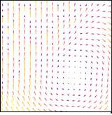
Figure 1: A vector field in $\mathcal{P}_{\@slowromancap v@}$.

To address the challenge of setting the complexity level of the prior class, we introduce an adaptive (learnable) construction scheme for a prior class. Let $w_{j}({\bm{x}},t):\mathbb{R}^{d}\times\mathbb{R}_{+}\rightarrow\mathbb{R}$, $1\leq j\leq k$, be learnable functions, which are part of the dynamic reconstruction model, i.e., $w_{j}(\cdot,t)\in\Psi_{t}$ and $w_{j}$ are normalized, i.e., $\sum_{j=1}^{k}w_{j}({\bm{x}},t)=1$. The details of $w_{j}$ architecture are left to Section 5. We can construct a complex prior class by assigning simpler prior classes to different parts of the space, according to the weights $w_{j}$. For example, let us consider a piece-wise rigid deformation prior class defined as:

$$\mathcal{P}_{\@slowromancap iv@}=\left\{u_{t}|u({\bm{x}},t)=\sum_{j=1}^{k}w_{j}({\bm{x}},t)u_{j}({\bm{x}},t),u_{j}\in\mathcal{P}_{\@slowromancap ii@}\text{ for }1\leq j\leq k,\sum_{j=1}^{k}w_{j}({\bm{x}},t)=1\right\}.$$ (23)

In a similar manner, we can also combine $\mathcal{P}_{\@slowromancap i@}$ with rigid deformations and derive a prior class defined as:

$$\mathcal{P}_{\@slowromancap v@}=\left\{u_{t}|u({\bm{x}},t)=\sum_{j=1}^{k}w_{j}({\bm{x}},t)u_{j}({\bm{x}},t),u_{1}\in\mathcal{P}_{\@slowromancap i@},u_{j}\in\mathcal{P}_{\@slowromancap ii@}\text{ for }2\leq j\leq k,\sum_{j=1}^{k}w_{j}({\bm{x}},t)=1\right\}.$$ (24)

Figure 1 illustrates an element in $\mathcal{P}_{\@slowromancap v@}$, with weights $w_{j}$ dividing the plane to a restricted up direction deformation above the diagonal, and a rigid deformation below the diagonal. Note that directly substituting an adaptive-combination prior class in 5 would no longer yield a linear problem. Therefore, we propose to use a linear problem that upper bounds the matching optimization problem of 5. For example, in the case of 9 with $\mathcal{P}_{\@slowromancap iv@}$, we can solve:

$$\min_{\left\{({\bm{A}}_{jt},{\bm{b}}_{jt})\right\}}\sum_{i=1}^{n}\sum_{j=1}^{k}w_{j}(\gamma_{t}^{i},t)\left\|{\bm{A}}_{jt}\gamma^{i}_{t}+{\bm{b}}_{jt}-\frac{d}{dt}\gamma^{i}_{t}\right\|^{2}\text{ s.t. }{\bm{A}}_{jt}=-{{\bm{A}}_{jt}}^{T}.$$ (25)

Using Jensen’s inequality, it can be seen that 25 upper bounds the matching optimization from 5. Again the minimization problem of 25 can be solved efficiently, as it corresponds to a weighted least squares problem that is solvable independently for each $j\in[k]$, similarly to 17.

Lastly, as incorporating $\mathcal{P}_{\@slowromancap ii@}$ in 5 involves a non standard least-squares problem which includes a constraint, we formulate the analytic solutions for $\mathcal{P}_{\@slowromancap iv@}$ in the next lemma, covering 17 and 18 as a special case.

Lemma 1.

For the prior class $\mathcal{P}_{\@slowromancap iv@}$, the solutions $({\bm{A}}_{jt},{\bm{b}}_{jt})$ to the minimization problem 25 are given by,

$$\left[\begin{array}[]{c}\mathrm{vech}({\bm{A}}_{jt})\\ {\bm{b}}_{jt}\end{array}\right]={\bm{P}}_{jt}^{-1}\left[\begin{array}[]{c}\mathrm{vec}(\dot{\bm{\Gamma}}_{t}^{T}{\bm{W}}_{jt}\bm{\Gamma}_{jt}-\bm{\Gamma}^{T}_{jt}{\bm{W}}_{jt}\dot{\bm{\Gamma}}_{t})\\ \frac{1}{{\bm{1}}^{T}{\bm{W}}_{jt}{\bm{1}}}{\bm{1}}^{T}{\bm{W}}_{jt}\dot{\bm{\Gamma}}_{t}\end{array}\right]$$

where $\bm{\Gamma}_{jt}=\left[\gamma^{1}_{t},\cdots,\gamma^{n}_{t}\right]^{T}\in\mathbb{R}^{n\times d}$, $\dot{\bm{\Gamma}}_{t}=\left[\frac{d}{dt}\gamma^{1}_{t},\cdots,\frac{d}{dt}\gamma^{n}_{t}\right]^{T}\in\mathbb{R}^{n\times d}$, ${\bm{W}}_{jt}=\sum_{i=1}^{n}w_{j}(\gamma^{i}_{t},t){\bm{e}}_{i}{\bm{e}}_{i}^{T}$ with $\left\{{\bm{e}}_{i}\right\}$ as the standard basis in $\mathbb{R}^{n}$, $\mathrm{vech}({\bm{A}}_{jt})\in\mathbb{R}^{\frac{d(d-1)}{2}}$ denotes the half-vectorization of the anti-symmetric matrix ${\bm{A}}_{jt}$, and the matrix ${\bm{P}}_{jt}^{-1}$ depends solely on $\bm{\Gamma}_{jt}$, $\dot{\bm{\Gamma}}_{t}$, and ${\bm{W}}_{jt}$.

The solutions $({\bm{A}}_{jt},{\bm{b}}_{jt})$ to the minimization problem 5 with 10 are given by,

$$\left[\begin{array}[]{c}\mathrm{vech}({\bm{A}}_{jt})\\ {\bm{b}}_{jt}\end{array}\right]={\bm{P}}_{jt}^{-1}\left[\begin{array}[]{c}\sum_{i=1}^{n}w_{j}({\bm{x}}_{i},t)\mathrm{vec}(s_{i}({\bm{x}}_{i}[{\bm{g}}_{t}^{i}]^{T}-{\bm{g}}_{t}^{i}{\bm{x}}_{i}^{T}))\\ {\bm{G}}_{t}^{T}{\bm{W}}_{jt}{\bm{s}}\end{array}\right]$$

where ${\bm{g}}_{t}^{i}=[\nabla\psi_{t}({\bm{x}}_{i})]^{T}$, $\bm{G}_{t}=\left[{\bm{g}}^{1}_{t},\cdots,{\bm{g}}^{n}_{t}\right]^{T}\in\mathbb{R}^{n\times d}$, $s_{i}=\frac{\partial}{\partial{t}}\psi_{t}({\bm{x}}_{i})$, ${\bm{s}}=\left[s^{1}_{t},\cdots,s^{n}_{t}\right]^{T}\in\mathbb{R}^{n}$.

For the proof of lemma 1, including the details of ${\bm{P}}_{jt}^{-1}$ computation, we refer the reader to the Appendix.

5 Implementation details

In this section, we provide additional details about the dynamic image model $\Psi_{t}$ employed in this work, based on Gaussian Splatting (Kerbl et al., 2023). We provide an overview of this image model, followed by details about the dynamic model used in the experiments.

Gaussian Splatting image model.

The Gaussian Splatting image model is parameterized by a collection of $n$ 3D Gaussians augmented with color and opacity parameters. That is, ${\bm{\theta}}=\left\{{\bm{\mu}}^{i},{\bm{\Sigma}}^{i},{\bm{c}}^{i},\alpha^{i}\right\}_{i=1}^{n}$ with ${\bm{\mu}}^{i}\in\mathbb{R}^{3}$ denoting the $i$^th Gaussian mean, ${\bm{\Sigma}}^{i}\in\mathbb{R}^{3\times 3}$ its covariance matrix, ${\bm{c}}^{i}\in\mathbb{R}^{3}$ its color, and $\alpha^{i}\in\mathbb{R}$ its opacity. To render an image, the 3D Gaussians are projected to the image plane to form a collection of 2D Gaussians parameterized by $\left\{{\bm{\mu}}^{i}_{\textrm{2D}},{\bm{\Sigma}}^{i}_{\textrm{2D}}\right\}$. Given $K,E$ denoting the intrinsic and extrinsic camera transformations, the image plane Gaussians parameters are calculated using the point rendering formula:

$$\mu^{i}_{\textrm{2D}}=K\frac{E\mu^{i}}{(E\mu^{i})_{{\bm{z}}}},$$ (26)

and,

$${\bm{\Sigma}}^{i}_{\textrm{2D}}=JE{\bm{\Sigma}}^{i}E^{T}J^{T},$$ (27)

where $J$ denotes the Jacobian of the affine transformation of 26. Lastly, an image pixel $I({\bm{p}})$ is obtained by alpha-blending the ordered by depth visible Gaussians:

$$I({\bm{p}})=\sum_{i=1}^{n}c^{i}\alpha^{i}\sigma^{i}\left({\bm{p}}\right)\prod_{j=1}^{i-1}\left(1-\alpha^{j}\sigma^{j}\left({\bm{p}}\right)\right),$$ (28)

where $\sigma^{i}({\bm{p}})=\exp{\left(-\frac{1}{2}\left({\bm{p}}-{\bm{\mu}}^{i}_{\textrm{2D}}\right)^{T}({\bm{\Sigma}}^{i}_{\textrm{2D}})^{-1}\left({\bm{p}}-{\bm{\mu}}^{i}_{\textrm{2D}}\right)\right)}$.

Dynamic image model.

We utilize the Gaussian Splatting image model to construct our dynamic model as:

$$\Psi_{t}=\left\{{\bm{\mu}}^{i}+{\bm{\mu}}^{i}(t),{\bm{\Sigma}}+{\bm{\Sigma}}^{i}(t),{\bm{c}}^{i},\alpha^{i},w_{ij}(t)\right\}_{i=1}^{n},$$ (29)

where ${\bm{\mu}}^{i}(t)=f_{{\bm{\mu}}}({\bm{\mu}}^{i},t)$, ${\bm{\Sigma}}^{i}(t)=f_{{\bm{\Sigma}}}({\bm{\mu}}^{i},t)$, $w_{ij}(t)={\bm{e}}_{j}^{T}\mathrm{softmax}(f_{w}({\bm{\mu}}^{i}+{\bm{\mu}}^{i}(t),{\bm{\mu}}^{i},t))$. We follow (Yang et al., 2023) and each of the functions: $f_{{\bm{\mu}}}:\mathbb{R}^{3}\times\mathbb{R}\rightarrow\mathbb{R}^{3}$, $f_{{\bm{\Sigma}}}:\mathbb{R}^{3}\times\mathbb{R}\rightarrow\mathbb{R}^{6}$, $f_{w}:\mathbb{R}^{3}\times\mathbb{R}^{3}\times\mathbb{R}\rightarrow\mathbb{R}^{k}$ is a Multilayer perceptron (MLP). For more details regarding the MLP architectures, we refer the reader to our Appendix. Note that the model element $w_{ij}(t)$ is only relevant to instances where the adaptive-combination prior class is assumed. Lastly, in our experiments we apply the ReMatching loss for ${\bm{\mu}}^{i}+{\bm{\mu}}^{i}(t)$, and for time-dependent rendered images $I_{t}$.

Training details.

We follow the training protocol of (Yang et al., 2023). We initialize the model using $n=100$K 3D Gaussians. Training is done for $40$K iterations, where for the first $3$K iterations, only $\left\{{\bm{\mu}}^{i},{\bm{\Sigma}}^{i},{\bm{c}}^{i},\alpha^{i}\right\}_{i=1}^{n}$ are optimized. In instances where the adaptive-combination prior class is applied, we supplement the ReMatching optimization objective with an entropy loss on the weights $w_{ij}$ as follows:

$$L_{\textrm{entropy}}=\frac{1}{k}\sum_{j=1}^{k}\frac{1}{n}\sum_{i=1}^{n}w_{ij}\log\left(\frac{1}{n}\sum_{i=1}^{n}w_{ij}\right).$$ (30)

Lastly, for all the experiments considered in this work, we set the ReMatching loss weight $\lambda=0.001$. Additional details are provided in the Appendix.

6 Experiments

		Bouncing Balls				Hell Warrior				Hook				JumpingJacks
Method		LPIPS $\downarrow$	PSNR $\uparrow$	SSIM $\uparrow$		LPIPS $\downarrow$	PSNR $\uparrow$	SSIM $\uparrow$		LPIPS $\downarrow$	PSNR $\uparrow$	SSIM $\uparrow$		LPIPS $\downarrow$	PSNR $\uparrow$	SSIM $\uparrow$
K-Planes (Fridovich-Keil et al., 2023)		0.0322	40.05	0.9934		0.0824	24.58	0.9520		0.0662	28.12	0.9489		0.0468	31.11	0.9708
D3G (Yang et al., 2023)		0.0089	41.52	0.9978		0.0261	41.28	0.9928		0.0165	37.03	0.9906		0.0137	37.59	0.9930
GA3D (Lu et al., 2024)		0.0093	40.76	0.9950		0.0210	41.30	0.9871		0.0124	37.78	0.9887		0.0121	37.00	0.9887
NPG (Das et al., 2024)						0.0537	38.68	0.9780		0.0460	33.39	0.9735		0.0345	33.97	0.9828
Ours - $\mathcal{P}_{\@slowromancap iii@}$		0.0087	41.84	0.9979		0.0244	41.59	0.9932		0.0161	37.19	0.9909		0.0134	37.72	0.9931
Ours - $\mathcal{P}_{\@slowromancap iv@}$ or $\mathcal{P}_{\@slowromancap v@}$		0.0089	41.61	0.9978		0.0245	41.69	0.9977		0.0158	37.39	0.9911		0.0131	38.01	0.9934
		Lego				Mutant				Stand Up				T-Rex
Method		LPIPS $\downarrow$	PSNR $\uparrow$	SSIM $\uparrow$		LPIPS $\downarrow$	PSNR $\uparrow$	SSIM $\uparrow$		LPIPS $\downarrow$	PSNR $\uparrow$	SSIM $\uparrow$		LPIPS $\downarrow$	PSNR $\uparrow$	SSIM $\uparrow$
K-Planes (Fridovich-Keil et al., 2023)		0.0331	25.48	0.9480		0.0362	32.50	0.9713		0.0310	33.10	0.9793		0.0343	30.43	0.9737
D3G (Yang et al., 2023)		0.0453	24.93	0.9537		0.0066	42.09	0.9966		0.0083	43.85	0.9970		0.0105	37.89	0.9956
GA3D (Lu et al., 2024)		0.0446	24.87	0.9420		0.0050	42.39	0.9951		0.0062	43.96	0.9948		0.0100	37.70	0.9929
NPG (Das et al., 2024)		0.0716	24.63	0.9312		0.0311	36.02	0.9840		0.0257	38.20	0.9889		0.0310	32.10	0.9959
Ours - $\mathcal{P}_{\@slowromancap iii@}$		0.0503	24.89	0.9522		0.0067	42.13	0.9966		0.0085	43.99	0.9969		0.0105	38.07	0.9958
Ours - $\mathcal{P}_{\@slowromancap iv@}$ or $\mathcal{P}_{\@slowromancap v@}$		0.0456	24.95	0.9537		0.0065	42.40	0.9968		0.0081	44.31	0.9971		0.0103	38.38	0.9961

Table 1: Image quality evaluation on unseen frames for the D-NeRF dataset (Pumarola et al., 2021).

We evaluate the ReMatching framework on benchmarks involving synthetic and real-world video captures of deforming scenes. For quantitative analysis in both cases, we report the PSNR, SSIM (Wang et al., 2004)and LPIPS (Zhang et al., 2018) metrics.

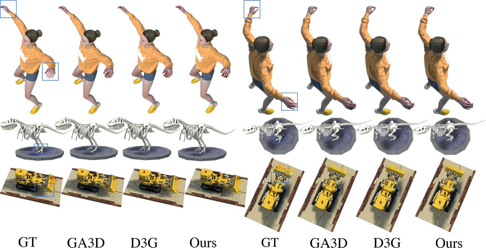
Figure 2: Qualitative comparison of baselines and our model on the D-NeRF dataset (Pumarola et al., 2021). We note that our framework consistently produces high fidelity reconstructions, accurately capturing fine-grained details, as highlighted in the blue boxes.

D-NeRF synthetic.

D-NeRF dataset (Pumarola et al., 2021) comprises of 8 scenes, each consisting from $100$ to $200$ frames, hence providing a dense multi-view coverage of the scene. We follow D-NeRF’s evaluation protocol and use the same train/validation/test split at $800\times 800$ image resolution with a black background. In terms of baseline methods, we consider recent state-of-the-art dynamic models, including Deformable3DGaussians (D3G) (Yang et al., 2023), 3D Geometry-aware Deformable Gaussians (DAG) (Lu et al., 2024), Neural Parametric Gaussians (NPA) (Das et al., 2024), and K-Planes (Fridovich-Keil et al., 2023). Note that some of these baselines incorporate prior regularization losses such as local rigidity and smoothness to their optimization procedure. Table 1 summarizes the average image quality results for unseen frames in each scene. We include two variants of our framework: i) Using the divergence-free prior $\mathcal{P}_{\@slowromancap iii@}$; and ii) Using the adaptive-combination prior class $\mathcal{P}_{\@slowromancap iv@}$ or the class $\mathcal{P}_{\@slowromancap v@}$ specifically for scenes that include a floor component. Figure 2 provides a qualitative comparison of rendered test frames, highlighting the improvements of our approach, which: i) produces plausible reconstructions that avoid unrealistic distortions, e.g., the human fingers in the jumping jacks scene; ii) reduces rendering artifacts of extraneous parts, especially in moving parts such as the leg in the T-Rex scene.

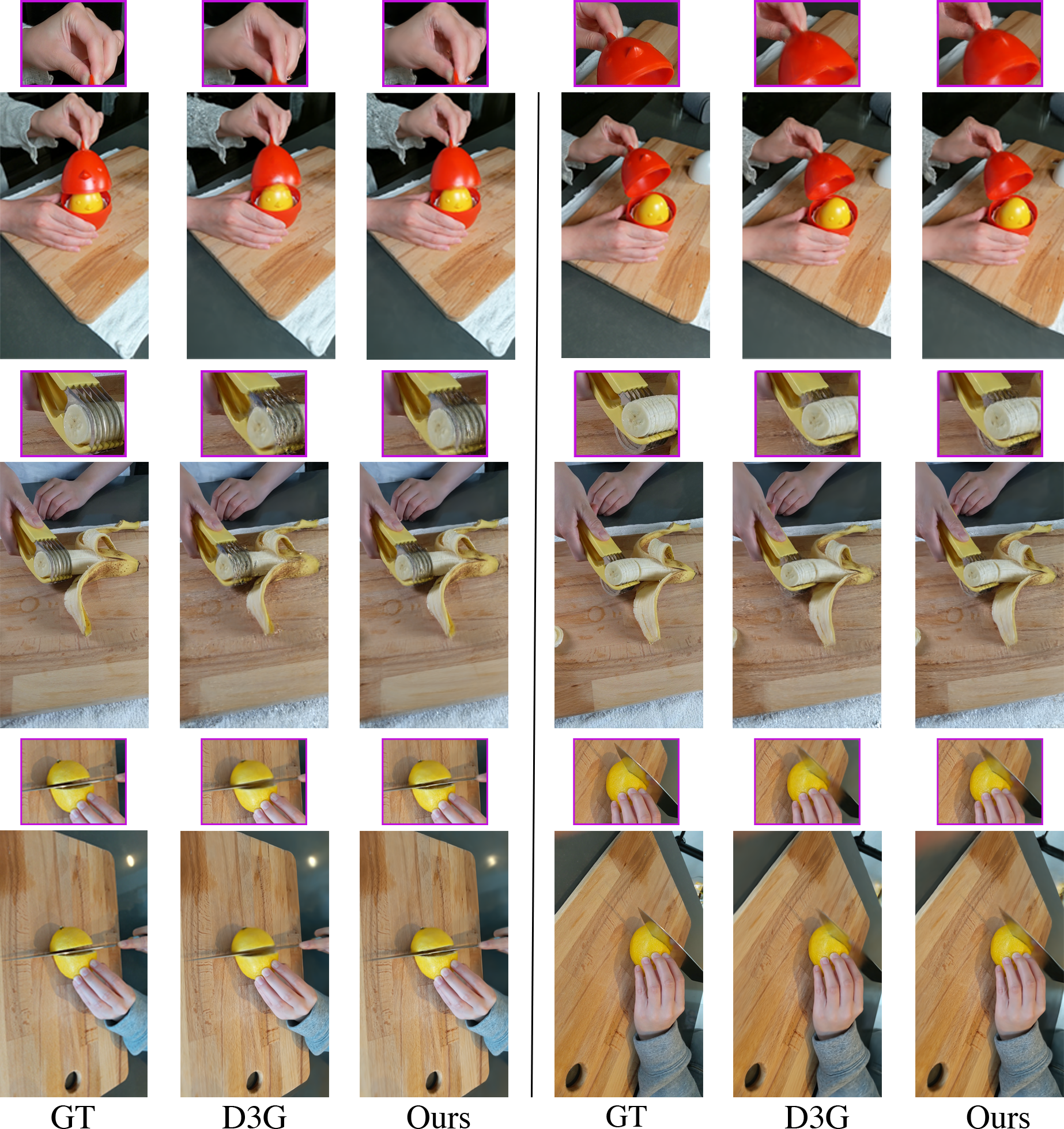
Figure 3: Qualitative comparison of our method to D3G (Yang et al., 2023) on the HyperNeRF dataset (Park et al., 2021b). Our framework yields more accurate reconstructions, in particular around moving parts.

HyperNeRF real-world.

Scene LPIPS $\downarrow$ PSNR $\uparrow$ SSIM $\uparrow$ Slice Banana D3G 0.3692 24.87 0.7935 Ours 0.3673 25.28 0.8025 Chicken D3G 0.3030 26.66 0.8813 Ours 0.3044 26.80 0.8835 Lemon D3G 0.2858 28.65 0.8873 Ours 0.2675 28.30 0.8883 Torch D3G 0.2340 25.41 0.9207 Ours 0.2260 25.62 0.9229 Split Cookie D3G 0.0971 32.61 0.9657 Ours 0.0937 32.67 0.9667

Table 2: Unseen frames evaluation for the HyperNeRF dataset (Park et al., 2021b).

The HyperNeRF dataset (Park et al., 2021b) consists of real-world videos capturing a diverse set of human activities involving interactions with common objects. We follow the evaluation protocol provided with the dataset, and use the same train/test split. In table 2 we report image quality results for unseen frames on 5 scenes from the dataset: Slice Banana, Chicken, Lemon, Torch, and Split Cookie. Figure 3 shows qualitative comparison to the baseline D3G (Yang et al., 2023). Our approach demonstrates similar types of improvements as noticed in the synthetic case providing more realistic reconstructions, especially in areas involving deforming parts.

Adaptive-combination prior class.

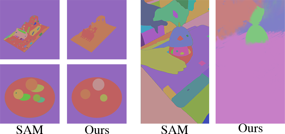
Figure 4: Part assignments for the adaptive-combination prior class.

Employing the adaptive-combination prior classes $\mathcal{P}_{\@slowromancap iv@}$ and $\mathcal{P}_{\@slowromancap v@}$ with learnable parts assignments $\left\{w_{ij}\right\}$ raises the question of whether the learning process successfully produced assignments $\left\{w_{ij}\right\}$ that align with the scene segmentation based on its deforming parts. Figure 4 shows our results for test frames from the Bouncing-Balls and Lego synthetic scenes (left), and the Chicken real-world scene (right). For comparison, we include the results of the Segment Anything Model (SAM) (Kirillov et al., 2023), which tends to over-segment the scene, mostly influenced by color variations and unable to capture the underlying geometry effectively.

ReMatching time-dependent image.

In this experiment we validate the applicability of the ReMatching loss for controlling model solutions via rendered images. To that end, we apply our framework with the $\mathcal{P}_{\@slowromancap iii@}$ prior class to the Jumping Jacks scene from D-NeRF on a single specific front view through time. The qualitative comparison to 3DG (Yang et al., 2023), as shown in the Appendix, supports the benefits of prior integration in this case as well, demonstrating more plausible reconstructions in areas involving moving parts.

7 Conclusions

We presented the ReMatching framework for integrating priors into dynamic reconstruction models. Our experimental results align with our hypothesis that the proposed ReMatching loss can induce solutions that match the required prior while achieving high fidelity reconstruction. We believe that the generality with which the framework was formulated would enable broader applicability to various dynamic reconstruction models. An interesting research venue is the construction of velocity-field-based prior classes emerging from video generative models, possibly utilizing our ReMatching formulation for time-dependent image intensity values. Another potential direction is the design of richer prior classes to handle more complex physical phenomena, such as ones including liquids and gases.

8 Appendix

8.1 Proofs

8.1.1 Proof of Lemma 1

Proof.

(Lemma 1)

Let $\bm{\Gamma}_{t}$, $\dot{\bm{\Gamma}}_{t}$, ${\bm{W}}_{jt}$ be given. Without loss of generality, we show the proof only for individuals $j\in[k]$ and $t$. So in order to ease the notation, in what follows we omit the subscripts $t$ and $j$. Let ${\bm{A}}\in\mathbb{R}^{d\times d}$ and ${\bm{b}}\in\mathbb{R}^{d}$, and define $[w_{1},\cdots,w_{n}]^{T}={\bm{W}}{\bm{1}}$. First, we show that $\sum_{i=1}^{n}w_{i}\left\|{\bm{A}}\gamma^{i}+{\bm{b}}-\dot{\gamma}^{i}\right\|^{2}$ can be reformulated as a weighted norm-squared minimization problem in ${\bm{A}}$ and ${\bm{b}}$. That is,

$$\sum_{i=1}^{n}w_{i}\left\|{\bm{A}}(\gamma^{i}-{\bm{c}})+{\bm{b}}-\dot{\gamma}^{i}\right\|^{2} =\sum_{i=1}^{n}\textrm{tr}{{\bm{A}}\sqrt{w_{i}}\gamma^{i}\sqrt{w_{i}}{\gamma{{}^{i}}}^{T}{\bm{A}}^{T}}-$$ (31)

$$2\textrm{tr}{\sqrt{w_{i}}(\dot{\gamma}^{i}-{\bm{b}})\sqrt{w_{i}}\gamma^{i}{\bm{A}}^{T}}+\textrm{tr}{\sqrt{w_{i}}(\dot{\gamma}^{i}-{\bm{b}})\sqrt{w_{i}}(\dot{\gamma}^{i}-{\bm{b}})^{T}}$$ (32)

$$=\textrm{tr}{{\bm{A}}\bm{\Gamma}^{T}{\bm{W}}\bm{\Gamma}{\bm{A}}^{T}}-2\textrm{tr}{(\dot{\bm{\Gamma}}-{\bm{1}}{\bm{b}}^{T})^{T}{\bm{W}}\bm{\Gamma}{\bm{A}}^{T}}+$$ (33)

$$\textrm{tr}{(\dot{\bm{\Gamma}}-{\bm{1}}{\bm{b}}^{T})^{T}{\bm{W}}(\dot{\bm{\Gamma}}-{\bm{1}}{\bm{b}}^{T})}$$ (34)

$$=\left\|\sqrt{{\bm{W}}}\left(\bm{\Gamma}{\bm{A}}^{T}-(\dot{\bm{\Gamma}}-{\bm{1}}{\bm{b}}^{T})\right)\right\|^{2}.$$ (35)

Next, we consider the following optimization problem:

$$\min_{{\bm{A}},{\bm{b}}}\left\|\sqrt{{\bm{W}}}\left(\bm{\Gamma}{\bm{A}}^{T}-(\dot{\bm{\Gamma}}-\mathbf{1}{\bm{b}}^{T})\right)\right\|^{2}\textrm{s.t. }{\bm{A}}=-{\bm{A}}^{T}.$$ (36)

Use the fact that ${\bm{A}}=-{\bm{A}}^{T}$ to define the following Lagrangian,

$$\mathcal{L}({\bm{A}},{\bm{b}},\Lambda)=\left\|\sqrt{{\bm{W}}}\left(\bm{\Gamma}{\bm{A}}-{\bm{1}}{\bm{b}}^{T}+\dot{\bm{\Gamma}}\right)\right\|^{2}+\textrm{tr}{\bm{\Lambda}^{T}({\bm{A}}+{\bm{A}}^{T})}$$ (37)

Then,

$$\frac{\partial{\mathcal{L}}}{\partial{A}}=2\bm{\Gamma}^{T}{\bm{W}}(\bm{\Gamma}{\bm{A}}-{\bm{1}}{\bm{b}}^{T}+\dot{\bm{\Gamma}})+\bm{\Lambda}+\bm{\Lambda}^{T}$$

Thus, $\frac{\partial{\mathcal{L}}}{\partial{{\bm{A}}}}=0$ yields that $\bm{\Gamma}^{T}{\bm{W}}(\bm{\Gamma}{\bm{A}}-{\bm{1}}{\bm{b}}^{T}+\dot{\bm{\Gamma}})$ is symmetric. Then, using again the fact that ${\bm{A}}=-{\bm{A}}^{T}$, we get that,

$$\bm{\Gamma}^{T}{\bm{W}}\bm{\Gamma}{\bm{A}}+{\bm{A}}\bm{\Gamma}^{T}{\bm{W}}\bm{\Gamma}+{\bm{b}}{\bm{1}}^{T}{\bm{W}}\bm{\Gamma}-\bm{\Gamma}^{T}{\bm{W}}{\bm{1}}{\bm{b}}^{T} =\dot{\bm{\Gamma}}^{T}{\bm{W}}\bm{\Gamma}-\bm{\Gamma}^{T}{\bm{W}}\dot{\bm{\Gamma}}.$$ (38)

Now, taking the derivative w.r.t. to ${\bm{b}}$ gives,

$$\frac{\partial{\mathcal{L}}}{\partial{{\bm{b}}}}=-2{\bm{1}}^{T}{\bm{W}}(\bm{\Gamma}{\bm{A}}-{\bm{1}}{\bm{b}}^{T}+\dot{\bm{\Gamma}})$$

and, $\frac{\partial{\mathcal{L}}}{\partial{{\bm{b}}}}=0$, yields that,

$$-\widehat{{\bm{w}}}^{T}\bm{\Gamma}{\bm{A}}+{\bm{b}}^{T}=\widehat{{\bm{w}}}^{T}\dot{\bm{\Gamma}},$$ (39)

where $\widehat{{\bm{w}}}=\frac{{\bm{W}}{\bm{1}}}{{\bm{1}}^{T}{\bm{W}}{\bm{1}}}$. Vectorizing the LHS of 38 gives,

$$\left(I_{d}\otimes\bm{\Gamma}^{T}{\bm{W}}\bm{\Gamma}+\bm{\Gamma}^{T}{\bm{W}}\bm{\Gamma}\otimes I_{d}\right)D_{d}\mathrm{vech}({\bm{A}})+\left(\bm{\Gamma}^{T}{\bm{W}}{\bm{1}}\otimes I_{d}-I_{d}\otimes\bm{\Gamma}^{T}{\bm{W}}{\bm{1}}\right){\bm{b}}$$ (40)

where $D_{d}$ is the duplication matrix transforming $\mathrm{vech}({\bm{A}})$ to $\mathrm{vec}({\bm{A}})$, with $\mathrm{vech}({\bm{A}})$ denoting the half-vectorization of the anti-symmetric matrix ${\bm{A}}$. Similarly, vectorizing the LHS of 39 yields,

$$-\frac{1}{{\bm{1}}^{T}{\bm{W}}{\bm{1}}}\left(I_{d}\otimes{\bm{1}}^{T}{\bm{W}}\bm{\Gamma}\right)D_{d}\mathrm{vech}(A)+{\bm{b}}.$$ (41)

Based on 40 and 41, we can define the following block matrix:

$${\bm{P}}=\left[\begin{array}[]{c|c}{\bm{Q}}={\bm{Q}}^{\prime}D_{d}&{\bm{R}}=\bm{\Gamma}^{T}{\bm{W}}{\bm{1}}\otimes I_{d}-I_{d}\otimes\bm{\Gamma}^{T}{\bm{W}}{\bm{1}}\\ \hline\cr{\bm{S}}={\bm{S}}^{\prime}D_{d}&{\bm{T}}=I_{d}\end{array}\right]$$ (42)

where ${\bm{Q}}^{\prime}=I_{d}\otimes\bm{\Gamma}^{T}{\bm{W}}\bm{\Gamma}+\bm{\Gamma}^{T}{\bm{W}}\bm{\Gamma}\otimes I_{d}$, and, ${\bm{S}}^{\prime}=-\frac{1}{{\bm{1}}^{T}{\bm{W}}{\bm{1}}}\left(I_{d}\otimes{\bm{1}}^{T}{\bm{W}}\bm{\Gamma}\right)$. Then, let,

$${\bm{U}} =({\bm{Q}}-{\bm{R}}{\bm{T}}^{-1}{\bm{S}})^{-1}=L_{d}\left({\bm{Q}}^{\prime}-{\bm{R}}{\bm{S}}^{\prime}\right)^{-1}$$ (43)

where $L_{d}$ is the matrix satisfying $D_{d}L_{d}=I_{d^{2}}$. Consequently,

$${\bm{P}}^{-1}=\left[\begin{array}[]{c|c}{\bm{U}}&-{\bm{U}}{\bm{R}}\\ \hline\cr-{\bm{S}}^{\prime}\left({\bm{Q}}^{\prime}-{\bm{R}}{\bm{S}}^{\prime}\right)^{-1}&I_{d}+{\bm{S}}^{\prime}\left({\bm{Q}}^{\prime}-{\bm{R}}{\bm{S}}^{\prime}\right)^{-1}{\bm{R}}\end{array}\right]$$ (44)

and,

$$\left[\begin{array}[]{c}\mathrm{vech}({\bm{A}})\\ {\bm{b}}\end{array}\right]={\bm{P}}^{-1}\left[\begin{array}[]{c}\mathrm{vec}(\dot{\bm{\Gamma}}^{T}{\bm{W}}\bm{\Gamma}-\bm{\Gamma}^{T}{\bm{W}}\dot{\bm{\Gamma}})\\ \widehat{{\bm{w}}}^{T}\dot{\bm{\Gamma}}\end{array}\right].$$ (45)

∎

Now, for the second part of the lemma. Let ${\bm{g}}_{i}=[\nabla\psi_{t}({\bm{x}}_{i})]^{T}$ , $s_{i}=\frac{\partial}{\partial{t}}\psi_{t}({\bm{x}}_{i})$. Consider the following energy,

$$L=\sum_{i=1}^{n}w_{i}\left({\bm{g}}_{i}^{T}\left(A{\bm{x}}_{i}+{\bm{b}}\right)+s_{i}\right)^{2}.$$ (46)

Note that,

$${\bm{g}}_{i}^{T}A{\bm{x}}_{i}={\bm{y}}_{i}^{T}{\bm{a}}$$ (47)

where ${\bm{a}}\coloneq\mathrm{vec}(A)$, and ${\bm{y}}_{i}\coloneq{\bm{x}}_{i}\otimes{\bm{g}}_{i}$. Then,

$$L =\sum_{i=1}^{n}w_{i}\left({\bm{a}}^{T}{\bm{y}}_{i}{\bm{y}}_{i}^{T}{\bm{a}}+{\bm{b}}^{T}{\bm{g}}_{i}{\bm{g}}_{i}^{T}{\bm{b}}+2{\bm{a}}^{T}{\bm{y}}_{i}{\bm{g}}_{i}^{T}{\bm{b}}+2{\bm{g}}_{i}^{T}s_{i}{\bm{b}}+2s_{i}{\bm{a}}^{T}{\bm{y}}_{i}+s_{i}^{2}\right).$$ (48)

Define the Lagrangian,

$$\mathcal{L}({\bm{a}},{\bm{b}},\lambda) ={\bm{a}}^{T}\sum_{i}{\bm{y}}_{i}w_{i}{\bm{y}}_{i}^{T}{\bm{a}}+{\bm{b}}^{T}{\bm{G}}^{T}{\bm{W}}{\bm{G}}{\bm{b}}+2{\bm{a}}^{T}\sum_{i}{\bm{y}}_{i}w_{i}{\bm{g}}_{i}^{T}{\bm{b}}+$$ (49)

$$2{\bm{s}}^{T}{\bm{W}}{\bm{G}}{\bm{b}}+2{\bm{a}}^{T}\sum_{i}w_{i}{\bm{y}}_{i}s_{i}+{\bm{t}}^{T}{\bm{W}}{\bm{t}}+\lambda^{T}({\bm{a}}+P{\bm{a}})$$ (50)

where $P$ is the permutation matrix s.t. $\mathrm{vec}(A^{T})=P{\bm{a}}$.

Then,

$$\frac{\partial{\mathcal{L}}}{\partial{{\bm{a}}}}=2\sum_{i}w_{i}{\bm{y}}_{i}{\bm{y}}_{i}^{T}{\bm{a}}+2\sum_{i}w_{i}{\bm{y}}_{i}{\bm{g}}_{i}^{T}{\bm{b}}+2\sum_{i}w_{i}{\bm{y}}_{i}s_{i}+\lambda+P\lambda$$ (51)

Equating the above to $0$ and unvectorizing it, yields the following matrix equation,

$$\sum_{i=1}^{n}w_{i}({\bm{g}}_{i}{\bm{g}}_{i}^{T}A{\bm{x}}_{i}{\bm{x}}_{i}^{T}+{\bm{g}}_{i}{\bm{g}}_{i}^{T}{\bm{b}}{\bm{x}}_{i}^{T}+s_{i}{\bm{g}}_{i}{\bm{x}}_{i}^{T})=\frac{1}{2}({\bm{\Lambda}}+{\bm{\Lambda}}^{T}),$$ (52)

yielding that the LHS is a symmetric matrix. Therefore,

$$\sum_{i=1}^{n}w_{i}({\bm{g}}_{i}{\bm{g}}_{i}^{T}A{\bm{x}}_{i}{\bm{x}}_{i}^{T}+{\bm{x}}_{i}{\bm{g}}_{i}^{T}{\bm{b}}{\bm{x}}_{i}^{T}+s_{i}{\bm{g}}_{i}{\bm{x}}_{i}^{T})=\sum_{i=1}^{n}w_{i}({\bm{x}}_{i}{\bm{x}}_{i}^{T}A^{T}{\bm{g}}_{i}{\bm{g}}_{i}^{T}+{\bm{x}}_{i}{\bm{b}}^{T}{\bm{g}}_{i}{\bm{g}}_{i}^{T}+s_{i}{\bm{x}}_{i}{\bm{g}}_{i}^{T}).$$ (53)

Rearranging the above and half-vectorizing both sides yields that,

$$\sum_{i=1}^{n}w_{i}({\bm{x}}_{i}{\bm{x}}_{i}^{T}\otimes{\bm{g}}_{i}{\bm{g}}_{i}^{T}+{\bm{g}}_{i}{\bm{g}}_{i}^{T}\otimes{\bm{x}}_{i}{\bm{x}}_{i}^{T})D_{d}\mathrm{vech}({\bm{A}})+w_{i}({\bm{x}}_{i}\otimes{\bm{g}}_{i}{\bm{g}}_{i}^{T}-{\bm{g}}_{i}{\bm{g}}_{i}^{T}\otimes{\bm{x}}_{i}){\bm{b}} =$$ (54)

$$\sum_{i=1}^{n}w_{i}\mathrm{vec}(s_{i}({\bm{x}}_{i}{\bm{g}}_{i}^{T}-{\bm{g}}_{i}{\bm{x}}_{i}^{T})).$$ (55)

Now,

$$\frac{\partial{\mathcal{L}}}{\partial{{\bm{b}}}}=0$$ (56)

yields that,

$${\bm{G}}^{T}{\bm{W}}{\bm{G}}{\bm{b}}+\sum_{i}w_{i}{\bm{g}}_{i}{\bm{y}}_{i}^{T}D_{d}\mathrm{vech}({\bm{A}})=-{\bm{G}}^{T}{\bm{W}}{\bm{s}}.$$ (57)

Therefore,

$${\bm{P}}=\left[\begin{array}[]{c|c}{\bm{Q}}={\bm{Q}}^{\prime}D_{d}&{\bm{R}}=\sum_{i=1}^{n}w_{i}({\bm{x}}_{i}\otimes{\bm{g}}_{i}{\bm{g}}_{i}^{T}-{\bm{g}}_{i}{\bm{g}}_{i}^{T}\otimes{\bm{x}}_{i})\\ \hline\cr{\bm{S}}={\bm{S}}^{\prime}D_{d}&{\bm{T}}={\bm{G}}^{T}{\bm{W}}{\bm{G}}\end{array}\right],$$ (58)

where ${\bm{S}}^{\prime}=\sum_{i=1}^{n}w_{i}{\bm{g}}_{i}{\bm{y}}_{i}^{T}$, and ${\bm{Q}}^{\prime}=\sum_{i=1}^{n}w_{i}({\bm{x}}_{i}{\bm{x}}_{i}^{T}\otimes{\bm{g}}_{i}{\bm{g}}_{i}^{T}+{\bm{g}}_{i}{\bm{g}}_{i}^{T}\otimes{\bm{x}}_{i}{\bm{x}}_{i}^{T})$. Then, let,

$${\bm{U}} =({\bm{Q}}-{\bm{R}}{\bm{T}}^{-1}{\bm{S}})^{-1}=L_{d}\left({\bm{Q}}^{\prime}-{\bm{R}}{\bm{T}}^{-1}{\bm{S}}^{\prime}\right)^{-1}$$ (59)

where $L_{d}$ is the matrix that satisfies $D_{d}L_{d}=I_{d^{2}}$. Consequently,

$${\bm{P}}^{-1}=\left[\begin{array}[]{c|c}{\bm{U}}&-{\bm{U}}{\bm{R}}{\bm{T}}^{-1}\\ \hline\cr-{\bm{T}}^{-1}{\bm{S}}^{\prime}\left({\bm{Q}}^{\prime}-{\bm{R}}{\bm{T}}^{-1}{\bm{S}}^{\prime}\right)^{-1}&{\bm{T}}^{-1}+{\bm{T}}^{-1}{\bm{S}}^{\prime}\left({\bm{Q}}^{\prime}-{\bm{R}}{\bm{T}}^{-1}{\bm{S}}^{\prime}\right)^{-1}{\bm{R}}{\bm{T}}^{-1}\end{array}\right].$$ (60)

8.2 Additional Implementation Details

8.2.1 Architecture

We first describe the construction of the Gaussian Splatting dynamic image model referenced in section 5. The time invariant base of the model is optimized throughout training and consists of the following set of parameters ${\bm{\theta}}=\left\{{\bm{\mu}}^{i},{\bm{S}}^{i},{\bm{R}}^{i},,{\bm{c}}^{i},\alpha^{i}\right\}_{i=1}^{n}$ with Gaussian mean ${\bm{\mu}}^{i}\in\mathbb{R}^{3}$, scaling ${\bm{S}}^{i}\in\mathbb{R}^{3}$, rotation quaternion ${\bm{R}}^{i}\in\mathbb{R}^{4}$, color ${\bm{c}}^{i}\in\mathbb{R}^{3}$ and opacity $\alpha^{i}\in\mathbb{R}$. The covariance matrix ${\bm{\Sigma}}^{i}$ is calculated during the rendering process from the temporally augmented scaling and rotation parameters.

The time dependent deformation model transforms the time invariant Gaussian mean ${\bm{\mu}}^{i}$ and selected time $t$ into the deformation of the mean, scaling, rotation and the model element $w$ in the case of the adaptive-combination prior.

We generate positional embeddings (Mildenhall et al., 2020) of the time and mean inputs, which we pass to the deformation model Multilayer perceptrons.

$$\mathrm{Emb_{time}}(t):\mathbb{R}\rightarrow\mathbb{R}^{d_{\text{time emb}}}$$

$$\mathrm{Emb_{mean}}(\mu^{i}):\mathbb{R}^{3}\rightarrow\mathbb{R}^{d_{\text{mean emb}}}$$

The deformation model is made up of layers of the form:

$$\mathrm{LIN}(n,d_{\text{in}},d_{\text{out}}):{\bm{X}} \mapsto\nu\left({\bm{X}}{\bm{W}}+\mathbf{1}{\bm{b}}^{T}\right)$$

where $\nu=\mathrm{Softplus}_{\beta}$, with $\beta=100$.

For the deformation of the mean, scaling and rotation, the model takes the same form with minor differences in the final layer depending on the deforming parameter.

$$\textrm{Emb}_{time}(t)\rightarrow\mathrm{LIN}(n,d_{\text{time emb}},256)\rightarrow\mathrm{LIN}(n,256,d_{\tau})\rightarrow\tau$$

$$[\tau,\textrm{Emb}_{mean}(\mu)]\rightarrow\mathrm{LIN}(n,{d_{\tau}}+{d_{\text{mean emb}}},256)\rightarrow\mathrm{LIN}(n,256,256)\rightarrow$$

$$\mathrm{LIN}(n,256,256)\rightarrow\mathrm{LIN}(n,256,256)\rightarrow[\tau,\textrm{Emb}_{mean}(\mu),\mathrm{LIN}(n,256,256)]\rightarrow$$

$$\mathrm{LIN}(n,{d_{\tau}}+{d_{\text{mean emb}}}+256,256)\rightarrow\mathrm{LIN}(n,256,256)]\rightarrow\mathrm{LIN}(n,256,256)]\rightarrow\omega$$

$$\textrm{Mean}:\omega\rightarrow\mathrm{LIN}(n,256,3)\rightarrow\mu(t)$$

$$\textrm{Scaling}:\omega\rightarrow\mathrm{LIN}(n,256,3)\rightarrow{\bm{S}}(t)$$

$$\textrm{Rotation}:\omega\rightarrow\mathrm{LIN}(n,256,4)\rightarrow{\bm{R}}(t)$$

For the prediction of the $w$ we use a shallower Multilayer perceptron.

$$[\tau,\textrm{Emb}_{mean}(\mu+\mu(t)),\textrm{Emb}_{mean}(\mu)]\rightarrow\mathrm{LIN}(n,{d_{\tau}}+2\cdot{d_{\text{mean emb}}},256)\rightarrow$$

$$\mathrm{LIN}(n,256,K)\rightarrow\mathrm{Softmax}\rightarrow w(t)$$

8.2.2 Hyperparameters and training details

We set $d_{\text{mean emb}}=63$, $d_{\text{time emb}}=13$ and $d_{\tau}=30$. For optimization we use an Adam optimizer with different learning rates for the network components, keeping the hyperparameters of the baseline model (Yang et al., 2023).

In the case of the adaptive-combination prior we select $k$ based on a hyperparameter search between 1 and 35. The optimal value for most scenes ranges between 5 and 15, though the number also depends on the selected composition of priors. For example, a single volume-preserving class can supervise multiple moving objects as opposed to a single rigid deformation class. We use the ReMatching loss weight $\lambda$ = 0.001. When supplementing the ReMatching loss with an additional entropy loss, we use 0.0001 as the entropy loss weight.

For derivative calculation we use the PyTorch Forward-mode Automatic Differentiation.

8.2.3 ReMatching rendered image

The reconstruction model architecture in the case of the image ReMatching is the same as for the other experiments. At initialization we select a fixed viewpoint for the evaluation of the image space loss, which is kept throughout training. At every iteration we sample a random time and evaluate the ReMatching loss from the fixed viewpoint.

For approximating equation 10, we calculate a sample by choosing points that their image value is close to $0$ after applying the following transformation:

$$f(x)=-0.1\cdot\ln(1-\left|x\right|)\cdot\operatorname{sign}(x)$$ (61)

on the image.

Next, we compute the image gradient using automatic differentiation and use our single class div-free solver to reconstruct the flow and calculate the loss. We apply the ReMatching loss with a weight of 0.0001.

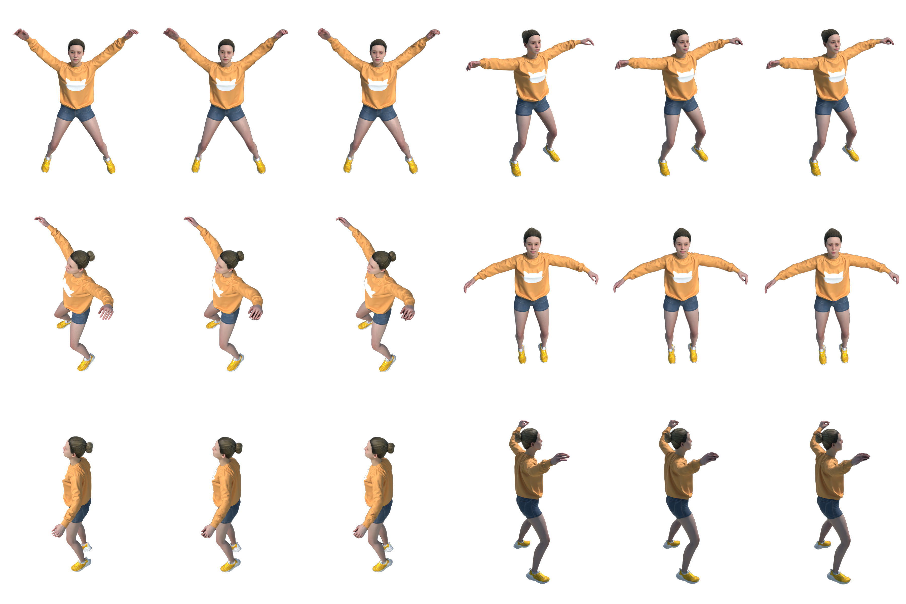
Figure 5: Qualitative comparison of the ReMatching loss applied in the image space. Each group of 3 is showing Ground-Truth (left), Ours (center), and 3DG (right).

References

- Albergo et al. (2023) Michael S. Albergo, Nicholas M. Boffi, and Eric Vanden-Eijnden. Stochastic interpolants: A unifying framework for flows and diffusions, 2023. URL https://arxiv.org/abs/2303.08797.
- Ben-Hamu et al. (2022) Heli Ben-Hamu, Samuel Cohen, Joey Bose, Brandon Amos, Aditya Grover, Maximilian Nickel, Ricky TQ Chen, and Yaron Lipman. Matching normalizing flows and probability paths on manifolds. arXiv preprint arXiv:2207.04711, 2022.
- Cao & Johnson (2023) Ang Cao and Justin Johnson. Hexplane: A fast representation for dynamic scenes. In Proceedings of the IEEE/CVF Conference on Computer Vision and Pattern Recognition, pp. 130–141, 2023.
- Chen et al. (2018) Ricky TQ Chen, Yulia Rubanova, Jesse Bettencourt, and David K Duvenaud. Neural ordinary differential equations. Advances in neural information processing systems, 31, 2018.
- Chu et al. (2022) Mengyu Chu, Lingjie Liu, Quan Zheng, Erik Franz, Hans-Peter Seidel, Christian Theobalt, and Rhaleb Zayer. Physics informed neural fields for smoke reconstruction with sparse data. ACM Trans. Graph., 2022.
- Das et al. (2024) Devikalyan Das, Christopher Wewer, Raza Yunus, Eddy Ilg, and Jan Eric Lenssen. Neural parametric gaussians for monocular non-rigid object reconstruction. In Proceedings of the IEEE/CVF Conference on Computer Vision and Pattern Recognition, pp. 10715–10725, 2024.
- Deutsch (1992) Frank Deutsch. The method of alternating orthogonal projections. In Approximation theory, spline functions and applications, pp. 105–121. Springer, 1992.
- Du et al. (2021) Yilun Du, Yinan Zhang, Hong-Xing Yu, Joshua B Tenenbaum, and Jiajun Wu. Neural radiance flow for 4d view synthesis and video processing. In 2021 IEEE/CVF International Conference on Computer Vision (ICCV), pp. 14304–14314. IEEE Computer Society, 2021.
- Eisenberger et al. (2019) Marvin Eisenberger, Zorah Lähner, and Daniel Cremers. Divergence-free shape correspondence by deformation. In Computer Graphics Forum, volume 38, pp. 1–12. Wiley Online Library, 2019.
- Fridovich-Keil et al. (2023) Sara Fridovich-Keil, Giacomo Meanti, Frederik Rahbæk Warburg, Benjamin Recht, and Angjoo Kanazawa. K-planes: Explicit radiance fields in space, time, and appearance. In IEEE/CVF Conference on Computer Vision and Pattern Recognition, CVPR 2023, Vancouver, BC, Canada, June 17-24, 2023, pp. 12479–12488. IEEE, 2023.
- Fridovich-Keil et al. (2023) Sara Fridovich-Keil, Giacomo Meanti, Frederik Rahbæk Warburg, Benjamin Recht, and Angjoo Kanazawa. K-planes: Explicit radiance fields in space, time, and appearance. In CVPR, 2023.
- Guo et al. (2023) Haoyu Guo, Sida Peng, Yunzhi Yan, Linzhan Mou, Yujun Shen, Hujun Bao, and Xiaowei Zhou. Compact neural volumetric video representations with dynamic codebooks. In Advances in Neural Information Processing Systems 36: Annual Conference on Neural Information Processing Systems 2023, NeurIPS 2023, New Orleans, LA, USA, December 10 - 16, 2023, 2023.
- Kerbl et al. (2023) Bernhard Kerbl, Georgios Kopanas, Thomas Leimkühler, and George Drettakis. 3d gaussian splatting for real-time radiance field rendering. ACM Transactions on Graphics, 42(4), July 2023. URL https://repo-sam.inria.fr/fungraph/3d-gaussian-splatting/.
- Kirillov et al. (2023) Alexander Kirillov, Eric Mintun, Nikhila Ravi, Hanzi Mao, Chloe Rolland, Laura Gustafson, Tete Xiao, Spencer Whitehead, Alexander C. Berg, Wan-Yen Lo, Piotr Dollár, and Ross Girshick. Segment anything. arXiv:2304.02643, 2023.
- Ling et al. (2024) Huan Ling, Seung Wook Kim, Antonio Torralba, Sanja Fidler, and Karsten Kreis. Align your gaussians: Text-to-4d with dynamic 3d gaussians and composed diffusion models. In IEEE/CVF Conference on Computer Vision and Pattern Recognition, CVPR 2023, Vancouver, BC, Canada, June 17-24, 2023. IEEE, 2024.
- Lipman et al. (2022) Yaron Lipman, Ricky TQ Chen, Heli Ben-Hamu, Maximilian Nickel, and Matt Le. Flow matching for generative modeling. arXiv preprint arXiv:2210.02747, 2022.
- Lombardi et al. (2021) Stephen Lombardi, Tomas Simon, Gabriel Schwartz, Michael Zollhöfer, Yaser Sheikh, and Jason M. Saragih. Mixture of volumetric primitives for efficient neural rendering. ACM Trans. Graph., 40(4):59:1–59:13, 2021.
- Lu et al. (2024) Zhicheng Lu, Xiang Guo, Le Hui, Tianrui Chen, Min Yang, Xiao Tang, Feng Zhu, and Yuchao Dai. 3d geometry-aware deformable gaussian splatting for dynamic view synthesis. arXiv preprint arXiv:2404.06270, 2024.
- Madry (2017) Aleksander Madry. Towards deep learning models resistant to adversarial attacks. arXiv preprint arXiv:1706.06083, 2017.
- Mildenhall et al. (2020) Ben Mildenhall, Pratul P. Srinivasan, Matthew Tancik, Jonathan T. Barron, Ravi Ramamoorthi, and Ren Ng. Nerf: Representing scenes as neural radiance fields for view synthesis. In ECCV, 2020.
- Niemeyer et al. (2019) Michael Niemeyer, Lars Mescheder, Michael Oechsle, and Andreas Geiger. Occupancy flow: 4d reconstruction by learning particle dynamics. In Proceedings of the IEEE/CVF International Conference on Computer Vision, pp. 5379–5389, 2019.
- Park et al. (2021a) Keunhong Park, Utkarsh Sinha, Jonathan T. Barron, Sofien Bouaziz, Dan B. Goldman, Steven M. Seitz, and Ricardo Martin-Brualla. Nerfies: Deformable neural radiance fields. In 2021 IEEE/CVF International Conference on Computer Vision, ICCV 2021, Montreal, QC, Canada, October 10-17, 2021, 2021a.
- Park et al. (2021b) Keunhong Park, Utkarsh Sinha, Peter Hedman, Jonathan T. Barron, Sofien Bouaziz, Dan B. Goldman, Ricardo Martin-Brualla, and Steven M. Seitz. Hypernerf: A higher-dimensional representation for topologically varying neural radiance fields. CoRR, abs/2106.13228, 2021b. URL https://arxiv.org/abs/2106.13228.
- Pumarola et al. (2021) Albert Pumarola, Enric Corona, Gerard Pons-Moll, and Francesc Moreno-Noguer. D-nerf: Neural radiance fields for dynamic scenes. In Proceedings of the IEEE/CVF Conference on Computer Vision and Pattern Recognition, pp. 10318–10327, 2021.
- Rempe et al. (2020) Davis Rempe, Tolga Birdal, Yongheng Zhao, Zan Gojcic, Srinath Sridhar, and Leonidas J. Guibas. Caspr: Learning canonical spatiotemporal point cloud representations. In Advances in Neural Information Processing Systems 33: Annual Conference on Neural Information Processing Systems 2020, NeurIPS 2020, December 6-12, 2020, virtual, 2020.
- Rezende & Mohamed (2015) Danilo Rezende and Shakir Mohamed. Variational inference with normalizing flows. In International conference on machine learning, pp. 1530–1538. PMLR, 2015.
- Song et al. (2023) Liangchen Song, Anpei Chen, Zhong Li, Zhang Chen, Lele Chen, Junsong Yuan, Yi Xu, and Andreas Geiger. Nerfplayer: A streamable dynamic scene representation with decomposed neural radiance fields. IEEE Transactions on Visualization and Computer Graphics, 29(5):2732–2742, 2023.
- Sorkine & Alexa (2007) Olga Sorkine and Marc Alexa. As-rigid-as-possible surface modeling. In Symposium on Geometry processing, volume 4, pp. 109–116. Citeseer, 2007.
- Tretschk et al. (2021) Edgar Tretschk, Ayush Tewari, Vladislav Golyanik, Michael Zollhöfer, Christoph Lassner, and Christian Theobalt. Non-rigid neural radiance fields: Reconstruction and novel view synthesis of a dynamic scene from monocular video. In 2021 IEEE/CVF International Conference on Computer Vision, ICCV 2021, Montreal, QC, Canada, October 10-17, 2021, 2021.
- Vu et al. (2022) Tuan-Anh Vu, Duc Thanh Nguyen, Binh-Son Hua, Quang-Hieu Pham, and Sai-Kit Yeung. Rfnet-4d: Joint object reconstruction and flow estimation from 4d point clouds. In Shai Avidan, Gabriel J. Brostow, Moustapha Cissé, Giovanni Maria Farinella, and Tal Hassner (eds.), Computer Vision - ECCV 2022 - 17th European Conference, Tel Aviv, Israel, October 23-27, 2022, Proceedings, Part XXIII, 2022.
- Wang et al. (2024) Chaoyang Wang, Peiye Zhuang, Aliaksandr Siarohin, Junli Cao, Guocheng Qian, Hsin-Ying Lee, and Sergey Tulyakov. Diffusion priors for dynamic view synthesis from monocular videos. CoRR, abs/2401.05583, 2024.
- Wang et al. (2004) Zhou Wang, Alan C Bovik, Hamid R Sheikh, and Eero P Simoncelli. Image quality assessment: from error visibility to structural similarity. IEEE transactions on image processing, 13(4):600–612, 2004.
- Wu et al. (2023) Guanjun Wu, Taoran Yi, Jiemin Fang, Lingxi Xie, Xiaopeng Zhang, Wei Wei, Wenyu Liu, Qi Tian, and Xinggang Wang. 4d gaussian splatting for real-time dynamic scene rendering. arXiv preprint arXiv:2310.08528, 2023.
- Yang et al. (2023) Ziyi Yang, Xinyu Gao, Wen Zhou, Shaohui Jiao, Yuqing Zhang, and Xiaogang Jin. Deformable 3d gaussians for high-fidelity monocular dynamic scene reconstruction. arXiv preprint arXiv:2309.13101, 2023.
- Yu et al. (2023) Hong-Xing Yu, Yang Zheng, Yuan Gao, Yitong Deng, Bo Zhu, and Jiajun Wu. Inferring hybrid neural fluid fields from videos. In Advances in Neural Information Processing Systems 36: Annual Conference on Neural Information Processing Systems 2023, NeurIPS 2023, New Orleans, LA, USA, December 10 - 16, 2023, 2023.
- Yunus et al. (2024) Raza Yunus, Jan Eric Lenssen, Michael Niemeyer, Yiyi Liao, Christian Rupprecht, Christian Theobalt, Gerard Pons-Moll, Jia-Bin Huang, Vladislav Golyanik, and Eddy Ilg. Recent trends in 3d reconstruction of general non-rigid scenes. In Computer Graphics Forum, pp. e15062. Wiley Online Library, 2024.
- Zhang et al. (2018) Richard Zhang, Phillip Isola, Alexei A Efros, Eli Shechtman, and Oliver Wang. The unreasonable effectiveness of deep features as a perceptual metric. In Proceedings of the IEEE conference on computer vision and pattern recognition, pp. 586–595, 2018.