A Massera-type Theorem on relative-periodic solutions for a second-order model of rectilinear locomotion
Abstract
We study the existence of a global periodic attractor for the reduced dynamics of a discrete toy model for rectilinear crawling locomotion, corresponding to a limit cycle in the shape and velocity variables. The body of the crawler consists of a chain of point masses, joined by active elastic links and subject to smooth friction forces, so that the dynamics is described by a system of second order differential equations. Our main result is of Massera-type, namely we show that the existence of a bounded solution implies the existence of the global periodic attractor for the reduced dynamics. In establishing this result, a contractive property of the dynamics of our model plays a central role. We then prove sufficient conditions on the friction forces for the existence of a bounded solution, and therefore of the attractor. We also provide an example showing that, if we consider more general friction forces, such as smooth approximations of dry friction, bounded solutions may not exist.
Mathematics Subject Classification (2020). Primary: 70K42; Secondary: 34D45, 37C60.
Keywords. Massera-type result, crawling locomotion, relative-periodic solution, gait, dissipative system, limit cycle
1 Introduction
Many mechanical systems are modeled by time-periodic ordinary differential equations in : consider, for instance, systems subject to a periodic forcing. Compared to autonomous systems, for which a qualitative analysis naturally starts from characterizing equilibria, in time-periodic systems a first fundamental step is often the more challenging search for periodic solutions and their stability properties.
A relevant contribution on this topic is due to Massera [26] in 1950. He proved that, in the scalar case , if there exists a solution of a -periodic equation which is well defined and bounded in an interval of the form , then such solution converges to a -periodic solution. In the same paper Massera proved that this result is valid also in the planar case under the mild (but sharp) additional assumption that all solutions are globally defined in future. For a nice recent presentation of Massera’s theorems see [29]. An analogous of Massera’s theorem was obtained for a special class of time periodic ordinary differential equations in for arbitrary in [37]. This class satisfies an additional assumption, expressed in terms of a suitable Lyapunov-like function.
Results that infer the existence of a periodic (or quasiperiodic) solution given the existence of a bounded one have been often referred to as Massera-type theorems. These theorems have been proposed in various settings, including functional functional differential equations [5, 38], generalized differential equation [11], PDEs [4, 25] and differential inclusions [16].
In this paper, we obtain a Massera-type result for the dynamics arising from a toy-model of crawling locomotion, namely Theorem 4.1. The model we consider, is illustrated in Figure 1 and consists of a chain of blocks on a line, with adjacent blocks being joined by elastic active (i.e changing rest length) links and friction forces opposing the motion of each block. The time-periodicity in the governing equations is associated with the gait adopted, i.e. the periodic pattern of “actions” performed by the crawler to move. More precisely, in our model, the gait consists of a periodic change in rest lengths of the links and possibly in the friction forces, which indirectly leads to a change in the shape of the crawler (which we will show to be only asymptotically periodic). Equivalently, each active link can be thought as an actuator with controlled periodic shape, connected to the blocks by an elastic element, acting analogously to a muscle-tendon system.
Simpler models without elasticity, so that each gait coincides with a prescribed periodic shape change of the crawler has also been considered [2, 10, 13]. We notice, however, that crawling animals, such as earthworms or inchworms, are generally soft bodied. Moreover, in recent years, the field of soft robotics has shown the most interest in these locomotion strategies (see [3] and the introduction in [12] for a quick discussion), where a deformable body is the principal component. Both these considerations make the elastic case worth to study.
The key feature of studying a locomotion model is that periodicity is not anymore what we expect asymptotically, since it would mean the inability of the gait to produce any advancement. A proper way to address this issue comes from geometrical mechanics, with the notion of relative-periodicity. The concept applies to flows on a manifold which are equivariant with respect to the action of a Lie Group , so that a reduced dynamics can be properly defined on the quotient . An orbit on is relative-periodic if its projection on is periodic. This means that a relative-periodic solution with initial state reaches, after a period, a state , where describes the action of an element .
This structure becomes simpler and intuitive in our basic model of crawling. The manifold is the phase space and the symmetry group consists of the rigid translations of the body along the line, since elastic forces depend only on the distances between the blocks and not on their absolute positions along the line. Relative-periodicity corresponds to periodicity for a reduced dynamics which describes the shape the crawler (i.e. relative distances between the blocks) and the velocity of each block. However, a relative-periodic motion of the crawler is not necessarily a periodic one when seen on the whole phase space : after a cycle the crawler might have advanced of a certain distance , so that the final state is a rigid translation by of the initial one, with which it shares shape and velocities.
The link between relative-periodicity and locomotion is well known [21]. The most famous examples, however, usually consider simplified models where, for any given time-periodic input, all solutions of the systems are relative-periodic: we mention, for instance, kinematic descriptions of wheeled robots or models for swimming at low Reynolds number [9, 21]. Yet, in most concrete situations relative-periodicity emerges only as an asymptotic behaviour of the system. Usually this relates with the relevance of inertia and/or elasticity in the equations governing locomotion, making an initial velocity and/or deformation incompatible with any relative-periodic solution of the system. In such situation what we might expect is a relative-periodic Massera type result: that is, every solution whose reduced dynamics on is bounded admits a limit cycle in . In our case, this will mean that every solution bounded in shape and velocity converges to a relative-periodic solution.
For crawling models analogous to the one of Figure 1, this type of asymptotic behaviour has been studied in [2, 10, 13, 40] assuming prescribed shape or in [6] at a quasistatic regime with dry friction. Both situations significantly reduce the dimension and the complexity of the system; in particular with prescribed shape the dynamics is described simply by a scalar first order differential equation.
In this paper we study instead the full system, where both elastic links and the inertia of the blocks are considered. The complication added by this framework lies not only in the higher dimensionality of the system, but also on the fact that, compared to the other cases, monotonicity properties of the friction forces are present only on a subspace, so they cannot be directly employed to obtain a contraction-type structure of the solutions.
Extending our view also to other locomotion models, the convergence to a limit relative-periodic behaviour has been observed for other models with prescribed shape, e.g. [32, 35], or for quasistatic models with an elastic body, studied only in a small-actuation limit perturbing the autonomous fully-passive system [1, 23, 28, 30, 39]. However, up to our knowledge, a full second-order dynamics with inertia and an elastic body has been considered until now only in [8], where a system of four masses in a tetrahedral structure with elastic links were studied, again with perturbative methods in the small-actuation limit. In this work, we prove instead our convergence results directly for the time-periodic system, allowing large deformations.
Massera-type results leave open two relevant questions, which we also address for our model: whether all bounded solutions converge to the same unique limit cycle and whether a bounded (on ) solution exists to start with.
The uniqueness of the limit cycle in models of crawling seems to be at least partially related to the strong monotonicity of the friction force-velocity laws [13]. In this paper, such a property is assumed in hypothesis (A4) and uniqueness of the limit behaviour is provided jointly with our Massera-type Theorem. However, strong monotonicity fails in some other relevant scenarios not considered here, e.g. for dry friction, and multiplicity of the limit behaviour has been observed in such a case for simplified versions of our model. Precisely, multiplicity of the limit velocity has been shown for a dynamic model with prescribed shape [13], whereas multiplicity of the limit cycle in the shape component can be found in a quasistatic setting [6].
Regarding the existence of a bounded solution, such property is often obtained by finding a suitable Lyapunov-like or guiding function which expresses some dissipation mechanism of the dynamical system. In these cases what is found is actually the existence of a bounded set in which all the solutions of our system eventually enter. This property of a dynamical system is called point dissipativity [19, 24]. Notice that when a contractive structure of solutions is present, as it is the case for our reduced dynamics, point dissipativity is actually equivalent to the existence of a solution bounded in future, instead of just a sufficient condition.
In this paper we prove the point dissipativity of the reduced dynamics in Lemma 5.3 under the additional assumption (A6), which introduces some symmetry in the model and requires a sufficiently stiff body. We also observe that boundedness can be easily deduced in the case of time-dependent viscous friction, cf. Theorem 5.1.
However, such property does not hold in general for our model of locomotion. In fact, in Section 4 we present an example of a system for which the reduced dynamics is unbounded (see Example 2). The friction forces considered in the example are bounded, so that they do not verify (A4), and there is an internal resonance which drives the the oscillations in the shape to infinity. This leaves open the question whether or not general strongly monotone friction forces overcome internal resonances, thus leading to a global limit cycle.
The paper is structured as follows. In Section 2, we introduce our model of rectilinear locomotion and its main structural assumptions, showing the global forward existence of solutions in Theorem 2.1. The definitions of relative-periodic solution and reduced dynamics for our rectilinear model are discussed in Section 3. In Section 4 we establish a Massera-type theorem for the reduced dynamics (Theorem 4.1), and give the corresponding result for the locomotion model (Corollary 4.2). We also establish the contractive property of the reduced dynamics (Theorem 4.3 and Corollary 4.4). This section concludes with the above mentioned example of divergent behaviour (Example 2). Section 5 discusses the results about point dissipativity of our model in the case of viscous friction (Theorem 5.1) or under suitable additional assumptions (equal masses, equal friction forces and sufficient stiffness of the links, see Theorem 5.2). Proofs of these results are provided in Section 6 and Section 7, respectively.
2 A model of rectilinear crawling locomotion
We now consider the mechanical system represented in Figure 1, consisting of a chain of blocks on a line. Each block has mass and position along the line , for (more generally, should be seen as the displacement of the block with respect to a given reference configuration, cf. Remark 4.5. Thus the state of the system is described by the column vector where the denotes the transposition operation. In what follows, for sake of simplicity, if and are are column vectors, we denote by the column vector . We introduce the inertia matrix
| (2.1) |
where denotes the standard euclidean inner product in , with associated norm . The evolution of our model is governed by following system of second order ODEs:
| (2.2) |
where denotes the gradient with respect to the variable, here represented for convenience as a column vector, and the dot denotes the (total) time-derivative .
In the model two types of forces are considered: friction forces, described by , and elastic forces, described by .
The vector function is of the form . This means that on each block is acting a friction force , where is the velocity of the -th block. Please notice that we have introduced friction using functions , so that the actual friction force is : we made this choice so that (2.2) resembles the custom notation for scalar damped oscillators. We make the following assumptions on :
-
(A1)
is a Carathéodory function333We recall that a function satisfies is a Carathéodory function if the following conditions hold: • for every the function is measurable in ; • for almost every the function is continuous in ; • for every compact set there exists a Lebesgue integrable function such that for every . and is -periodic in ;
-
(A2)
is locally Lipschitz continuous in uniformly in , namely, for every compact set there exist a constant such that for every and it holds ;
-
(A3)
for every and ;
-
(A4)
there exists such that
The first two are classical regularity assumptions, that can be equivalently reformulated by requiring the analogous properties on each component. The third one comes from the structure of friction forces: namely the force acting on a block is zero if the velocity of the block is zero. Assumption (A4) gives the strong monotonicity of each , which combined with (A3) guarantees that friction forces are always opposing motion.
Elastic forces are, as usual, introduced as , where is the elastic energy. Notice that we are considering a time-dependent elastic energy : it will account not only for deformations from the rest configuration, but also for the actuation on the system, described as a time-dependent change in the rest configuration.
The peculiarity of locomotion models is that the elastic energy does not depend on the whole configuration space, but can be seen as defined on the subspace identifying the shape of the locomotor. To be more precise, let us introduce the projection matrix given by
The matrix associates to each states the corresponding shape vector defined by
with components , for . We assume that
-
(A5)
the elastic energy has the form
where is a symmetric positive-definite matrix, defining the norm on , and is a -periodic function belonging to .
It will be convenient to express the elasticity matrix as an operator on the whole space of configurations , instead of on the smaller shape subspace. To do so, we set . We note that is positive semidefinite since it has rank . Hence, we have
| (2.3) |
Example 1.
The simplest example of this structure is the one shown in Figure 1, where we have active elastic links, all having the same elastic constant , joining each couple of consecutive blocks. In such a case we have , where denotes the identity matrix, and is the rest length of the -th link. Thus, the terms in the gradient in (2.3) take the form
A general positive definite matrix allows us to consider more general situation, where the links have different elasticity constants , or where more complex structures are present, with links joining also non adjacent blocks.
Under assumptions (A1) (A2), (A3), (A5), from the general theory of ODEs [19, Section 1.5] it follows that for any there exists a unique maximal generalized solution of (2.2) defined on an open interval containing such that We recall that a generalized solution of (2.2) is a function defined on a nondegenerate interval which belongs to (i.e. a function with absolutely continuous derivative ) which satisfies (2.2) almost everywhere in . Throughout the paper, solutions of differential equations are to be intended in this generalized sense.
The existence in future of all solutions of system (2.2) is guaranteed by the following result, where we replace (A4) with the more general assumption (A4enumi) on the friction forces.
Theorem 2.1.
The proof of Theorem 2.1 is given in Appendix A and is based on an energy estimate, adapting to our situation the approach of [14, Proposition 3.3].
In what follows, without loss of generality, we assume .
3 Relative-periodic solutions in rectilinear locomotion
Our dynamics (2.2) can be equivalently formulated on the phase space as a system of first order differential equations , namely
| (3.1) |
We notice that the vector field on defined by (3.1) is invariant for translations of the crawler. Namely, writing and for any , we have
| (3.2) |
for every .
More precisely, we should say that at each time the vector field is equivariant with respect to the group action of the symmetry group , where is the special Euclidean group on . Since the structures of , seen as a manifold, and of the symmetry group are trivial, in our presentation we will use the simpler formalism of classical differential equation theory.444For instance, in general should be seen as a vector field on the tangent space of and (3.2) should read , where is the pushforward of , which in our case corresponds to the identity and is therefore omitted.
Clearly, the invariance with respect to the action of the symmetry group is also inherited by the solutions of (3.1), namely if is a solution of (3.1), so is for every . Thus, it is reasonable to study the reduced problem on the quotient space .
This problem has a clear interpretation in our setting. Indeed, we notice that given two solutions and , there exists such that if and only if they have the same shape, i.e., , and the same velocities, i.e., . Thus, recalling that , the reduced problem on reads
| (3.3) |
In presence of a symmetry, it is often very natural and convenient to study directly the reduced system. However, some attention should be paid on how properties on the reduced system are related to those on the original one. In our case, we are concerned with periodicity. Given a solution of (3.1) and its projection solving (3.3), it is trivial that if is -periodic solution, then also it projection is -periodic. However, the converse does not hold. In an equivariant system with a symmetry group , solutions whose projection on the quotient space is periodic are called relative-periodic. Accordingly, for our locomotion model (2.2) we give the following definition.
Definition 3.1.
More precisely, we see that a solution of (2.2) is relative -periodic if and only if
-
•
its shape is -periodic
-
•
its velocity vector is -periodic.
It follows that if is relative -periodic, then for some , which is usually called geometric phase of the relative-periodic solution. In other words, relative-periodic solutions are periodic up to the action of an element of the symmetry group .
Notice that, given a periodic solution of (3.3), it is always possible to reconstruct a corresponding relative-periodic solution of (2.2).
Lemma 3.2.
Proof.
If, in addition is -periodic, then its derivative has zero mean on and consequently we have
showing that the geometric phase in (3.4) is well-defined. ∎
Equation (3.4) is usually called reconstruction equation.
We see now how well the notion of relative-periodicity grasps the intuitive notion of gait: to a prescribed -periodic actuation we associate a -periodic shape change and a geometric phase describing the displacement produced by each iteration of the actuation cycle. Classical periodicity would be a too strong notion: periodic solutions of (2.2) have a zero geometric phase, corresponding to an incompetent crawler that after each iteration of the gait returns to the initial position.
As discussed in the introduction, our goal is to show that, given a -periodic actuation, our model asymptotically attains as a relative-periodic evolution. The specific behaviour of the crawler we are aiming to prove is formalized in the following definition.
Definition 3.3.
We say that the locomotion model (2.2) has an unique, globally asymptotically stable, relative-periodic behaviour if both the following conditions hold.
We emphasize that the key ideas of this section apply to locomotion models and other mechanical systems in general. However, the possibility to express the reduced and reconstruction equations (3.3),(3.4) as equations respectively on and , rather than on less approachable manifolds, strongly relies on us considering a simple example of rectilinear locomotion. For instance, if our crawler, possibly with a more complex bi-dimensional body structure, were instead moving on the whole plane, the symmetry group would become , which includes not only translations but also rotations. We refer to [9] for a nice presentation on the structure of relative-periodicity for some models of locomotion in a 2D or 3D space, namely with symmetry group or . Remarkably, two types of relative-periodic solution emerge, depending on the chosen actuation: (bounded) quasi-periodic solutions and drifting solutions. According to the symmetry group involved, one type might be prevalent with respect to the other one.
4 A Massera-type Theorem
In this section we present a Massera-type result for our model of locomotion. We prove that for the reduced dynamics the existence of a bounded orbit implies the existence of a global periodic attractor, meaning that all solutions of the model converge asymptotically to the same shape and the same velocity. An example at the end of the section suggests that such bounded orbit may not exist. In Section 5 we discuss some sufficient conditions for the existence of a bounded solution of the reduced dynamics.
We first state our result for the reduced system (3.3).
Theorem 4.1.
As an immediate consequence of Theorem 4.1 we have the following corollary for the locomotion model (2.2).
Corollary 4.2.
Suppose that (A1) (A2), (A3), (A4), (A5) hold, and that system (2.2) admits a solution bounded in shape and velocity on , i.e., there exist a solution of (2.2) and a constant such that
| for every . |
Then Equation (2.2) admits a unique, globally asymptotically stable, relative -periodic behaviour in the sense of Definition 3.3.
In order to prove Theorem 4.1, we first show a contraction-type result for the reduced dynamics (3.3).
Theorem 4.3.
Proof.
We define the function
| (4.3) |
so that
| (4.4) |
for a.e. . Using the second equation in (3.3) for each solution we get
| (4.5) |
for a.e. . Combining (4.4) and (4.5) we obtain
| (4.6) |
a.e. , where the first inequality follows from (A4) and the second from the equivalence of norms in , for a suitable constant .
Let us now define the function
so that the estimate in (4.6) reads , a.e. . Taking into account (4.5) and (A4) we get
By the estimate in (4.6) we deduce that is decreasing and therefore for every . By (4.3) and the equivalence of norms in it follows that and are bounded on ; hence, there exists such that
We can now apply Theorem 4.5 in [34, pag. 287]555 We note that this theorem is a corollary of Lemma 4.3 in [34, pag. 286] and that both results are stated assuming suitable inequalities on the Dini derivatives of the functions involved. However, one can adapt in a quite direct manner the proof of the Lemma, and hence of the theorem, to our Carathéodory setting by replacing the Dini derivatives , defined everywhere on , with the derivatives of the absolutely continuous functions involved, defined almost everywhere on . with to the following first order system, obtained by considering two copies of system (3.3),
| (4.7) |
and conclude that
This proves (4.2b).
For , let us define
We prove first a weaker form of (4.2a), namely that, for every and every
| (4.8) |
Subtracting the fourth equation from the second one in (4.7) and integrating the result in the time interval we get for the -th component
| (4.9) |
where is the -th vector of the canonical basis of
By the already proven (4.2b), we deduce that for every there exist a such that, for every , it holds .
Let us define the compact set . Hence, for every and for every time we have . By (A2), for every and every
| (4.10) |
Thus, for every , every and every index , it holds
It follows that, for every , we have as and, consequently, . We observe that the matrix has maximum rank, i.e., it has rank : indeed, is an invertible square matrix, while is an matrix with maximum rank. Thus, it follows that as and, accordingly, (4.8).
It remains to show that the convergence (4.8) implies the stronger property (4.2a), i.e, . To do so, we proceed by contradiction. Suppose that there exists and a sequence such that for some . By the continuity of and , and by (4.2b), there exists a constant such that for every . Let us now choose such that . Thus
| (4.11) |
Since (4.11) holds for every , we get a contradiction with (4.8), proving (4.2a).
∎
We notice that also the following variation of Theorem 4.3 holds, where the bound on the velocity of one solution is replaced by the global Lipschitz continuity of the friction .
Corollary 4.4.
Proof.
The proof closely follows that of Theorem 4.3, with a minor adjustment. Specifically, we notice that the bound of Theorem 4.3 is required only to to construct the compact set where local Lipschitz continuity from (A2) can be employed to obtain the estimate (4.10). However, if global Lipschitz continuity is assumed instead, then (4.10) holds directly with replacing. ∎
We are now ready to prove our main result for the reduced system (3.3).
Proof of Theorem 4.1.
Let and be as in the statement of the theorem. Define the compact set
Fix and let be the solution of (3.3) such that . By Theorem (4.3), we have that there exists such that for any .
Then, system (3.3) is point dissipative, and by [31, Corollary 2.1] we get that system (3.3) admits a -periodic solution . In our setting such solution belongs to . Moreover, applying again Theorem 4.3, we see that every other solution of (3.3) converges to as , namely
| (4.12) |
Our proof is concluded. ∎
We end this section with an example which shows that the shape and the velocities of our locomotor may not be bounded on . The system considered in the example is such that the friction forces are globally bounded, so condition (A4) does not hold; notice, however, that this example covers smooth approximations of dry friction.
Example 2.


Consider equation (2.2) with , , , , and satisfying (A1), (A2), (A3), (A4enumi) and such that
| (4.13) |
The resulting system is
| (4.14) |
Let be any solution of system (4.14) and let
The corresponding shape is a solution of
| (4.15) |
All solutions of (4.15), and hence also , satisfy
| (4.16a) | |||
| (4.16b) | |||
In fact, any solution of (4.15) is of the form
where . Since
from (4.13) we have
Then, if we define the sequence , by the first inequality we get immediately
and (4.16a) follows. In a similar manner, using the second inequality with , one gets (4.16b). From this unbounded oscillatory character of solutions it follows also that the velocity is unbounded on .
We notice that Example 2 relies on an internal resonance of the system. If we eliminate the resonance by changing the period of the input, considering for example , the numerical simulations differ significantly and suggest the possible existence of a global periodic attractor.
Remark 4.5.
The Reader might be wondering why in Example 2 we considered a sign-changing shape , which might seem to lead to a change in the order of the blocks. Although mechanisms allowing such an inversion might be produced, a better explanation is available. While we refer for simplicity to as the position of the -th block, as already noticed it should properly be considered as the displacement with respect to a (constant) reference configuration . Hence, the actual position of the block is and therefore the actual signed-distance between consecutive blocks is , so that a negative does not necessarily mean the inversion of the blocks. Notice that any choice of the reference configuration leads to the very same dynamics (2.2), up to embedding the constant in , so our setting is not restrictive.
Clearly, these considerations allow the shape to fluctuate around zero, but do not exclude block-inversion for sufficiently large shape changes. However, in actual devices, we expect other phenomena, such as nonlinear elastic forces, plasticity or damage in the links, to occur for deformations smaller than the ones required for block-inversion, so that the latter is not a limiting factor for the range of validity of the model.
5 Existence of a limit relative-periodic behaviour
Theorem 4.1, like all Massera-type theorems in general, solves only half of the problem, leaving open the question of whether a solution of (3.3) bounded on exists. As we saw in Example 2, this may not be the case.
We will prove the existence of such a bounded solution, thus establishing the existence of an unique limit relative-periodic behaviour, in two special situations.
The first case we consider is that of time-dependent viscous forces, which we will analyse in detail in Section 6. Our main result, proved in Section 6, is the following.
Theorem 5.1.
Notice that (A1) (A2), (A3) are automatically satisfied by (5.1). Moreover, under (5.1), condition (A4) is equivalent to assume the existence of such that on . We remark that, for viscous friction, the dynamics of the system becomes linear and an explicit form of the solutions is available, which allows us to recover additional information on the system. In particular, in Proposition 6.1, we show that if the friction matrix is constant in time, then the geometric phase of the corresponding relative-periodic solution is zero. In other words, in its relative-periodic limit the crawler becomes incompetent, with each iteration of the gait returning the crawler to its initial state, namely . Notice that a time-dependent viscous friction, although not fitting most concrete examples, is a key feature in the locomotion of microscale hydrogel crawlers [22, 33].
Outside of the (linear) viscous case, the existence of a bounded solution is a much more challenging issue. We prove it for a special case, in which we assume that all the blocks have the same mass and the same friction law , and that the body is sufficiently stiff. More precisely, we make the following additional assumption:
-
(A6)
and , where is -Lipschitz continuous in uniformly in , and such that the Lipschitz constant satisfies
where denotes the minimum eigenvalue of .
We have the following result.
Theorem 5.2.
When dealing with systems that include a dissipation mechanism, the existence of one solution which is bounded forward in time, as required by Massera-type theorems, can be established by demonstrating the system’s point dissipativity, i.e. the existence of a compact global attractor. As previously mentioned, in our setting this approach is not restrictive, since by Theorem 4.3 the existence of such an attractor follows from the existence of one bounded orbit.
The following lemma gives a sufficient condition for the point dissipativity of system system (2.2).
Lemma 5.3.
6 Time-dependent viscous friction
In this section we consider the case of viscous friction as defined in (5.1); we first demonstrate Theorem 5.1 and then discuss some further properties of this special case.
Proof of Theorem 5.1.
We begin by noticing that, in this setting, if we let , system (3.3) is the linear system
| (6.1) |
where
We therefore have to prove the existence of a unique -periodic solution of (6.1) and that such is a global attractor of the dynamics.
Let and be two solutions of (6.1) and set . Thus, is a solution of the homogeneous -periodic system
| (6.2) |
By Corollary 4.4 we know that as ; therefore by [19, Theorem 7.1] all characteristic multipliers of (6.2) have modulus less than one (and correspondingly all characteristic exponents have negative real part) and, moreover, there exists , such that
In the linear setting, we can say something more specific about the asymptotic dynamics. Let us first introduce the center of mass of the system as , where is the total mass of the system.
It is well known that , where is the sum of the external forces acting on the system. In our case, since elastic forces are all internal, is the sum of the friction forces acting on each block, and therefore
| (6.3) |
Let us write and notice that
| (6.4) |
Since, for every , the difference can be expressed as the sum of the associated to all the links between the -th and the -th blocks, it follows that each function is a linear function of the shape ; in particular, there exists a (constant) matrix such that .
The solutions of this equation have the form
| (6.6) |
We now focus on the special case of a constant friction matrix , for which it holds .
Proposition 6.1.
Proof.
By Theorem 5.1, all relative-periodic solutions have the same shape and the same velocities , so in particular they have the same velocity of the center of mass and both and are -periodic. Then, writing , satisfies the differential equation
| (6.7) |
which can be thought of as corresponding to a locomotor with periodically prescribed shape subject to constant viscous friction. For such locomotors it was proved in [13, Example 3.4] that there exists a unique globally attracting -periodic solution which has zero average on the period. By uniqueness and we conclude that . This proves the first part of the statement.
As a consequence, for a generic solution, the sequence of differences converges to zero as . Since the arithmetic mean of the first terms of a converging sequence converges to the limit of the sequence as , the second part of the statement easily follows. ∎
The incompetence of a discrete model of crawler with constant viscous friction was already observed in [7] in the quasistatic case with prescribed shape, and later in [13] in the dynamic case with prescribed shape. Different improvements can be applied to the viscous case in order to attain true locomotion capability, such as a continuous body [7] or considering time-dependent viscous forces [13, Example 3.5]. In our framework, where shape is not prescribed and the elastic energy is considered, we provide the following example of an effective discrete model of crawler employing time-dependent viscous friction to achieve a nonzero limit average velocity.


Example 3.
Consider equation (2.2) with , , , , and . This leads to the system
| (6.8) |
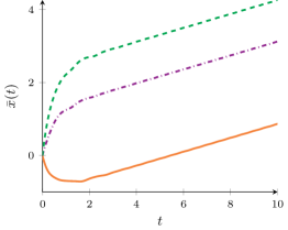
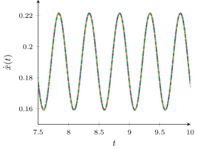
The simulation of system (6.8) for three different initial value problems is presented in Figure 3. We show the convergence for the shape (Fig. 3(a)) and for the velocity of the barycenter (Fig. 3(c)). Yet, favourable initial conditions might give a larger advancement of the position of the barycenter (Fig. 3(b)): we therefore remark that all solutions converge to the same relative-periodic behaviour (i.e. same limit in ), but not necessarily to exactly the same relative-periodic solution, namely the difference between the position of the barycenters of two solutions might converge to a nonzero constant.
We also observe that, while the shape converges to a -periodic cycle, the velocity of the barycenter seems to converge to a -periodic cycle (Fig. 3(d)). This can be explained by noticing that the locomotion strategy proposed partially resembles the so-called inching or two-anchor crawling [3, 12]. During each actuation period, there are two phases when the system pushes itself forward: during elongation friction is greater on the rear block, which works partially as an anchor pushing the front block forward, while the opposite happens during contraction, with the front block anchoring and pulling forward the other one.
7 Proof of Lemma 5.3
As a first step, we show that the shape and its time derivative both enter eventually a compact set independent of the initial values. Applying to both sides of (2.2) we get
| (7.1) |
where we have set . We introduce now the skewed energy function (see [18] for applications of this technique to synchronization problems):
| (7.2) |
where satisfies
| (7.3) |
The first upper bound on will be used later, the other two provide sufficient conditions for to be a positive-definite quadratic form. In particular, notice that the eigenvalues of are the values for (see [15, Example 7.4]), so that the smallest eigenvalue of satisfies . Hence, it holds
| (7.4) |
A computation of , i.e., the derivative of along the orbits, gives
Let us estimate each term individually. By (A4), we have
The second and third terms are bounded in norm by a linear term for some constant . The fourth will be controlled by the first one. For the fifth one, by Cauchy-Schwartz inequality we have
Thus, we have
| (7.5) |
where we recall that is the smallest eigenvalue of . By assumptions (A6) and (7.3) we have that the coefficients of the quadratic terms in the right-hand side of (7.5) are both negative. Hence the derivative along the orbit in a generic point satisfies
| (7.6) |
Let . By (7.6) we deduce that is bounded, and, by continuity of , compact. Let and set . Since , if follows that is forward invariant for the dynamics defined by (7.1) on . Moreover, for any given initial value (5.2), setting
we observe that the solution of (7.1) with initial conditions and satisfies for every .
To conclude the proof, let us introduce the center of mass of the system . As seen in Section 6, writing and , we have
| (7.7) |
Since, by (6.4), the are (constant) linear combinations of the , by the boundedness of the we know that there exists a constant such that, for every initial value problem (5.2), it holds for every and .
We now prove that, for every initial value problem (5.2), there exists a time , depending on , such that the corresponding solution satisfies
| (7.8) |
By (A4) and (7.7) we deduce that for almost every it holds
| (7.9) |
By (7.9) we deduce that if , then for every . Moreover, by (7.9) we also obtain that if , then
Thus, setting
it follows that (7.8) is satisfied and
Since is compact and is a (time-independent) linear transformation of in , the result follows. ∎
Acknowledgements.
Paolo Gidoni is a member of the Gruppo Nazionale di Fisica Matematica of the Istituto Nazionale di Alta Matematica. Alessandro Margheri was supported by FCT project UIDB/04561/2020: https://doi.org/10.54499/UIDB/04561/2020 . The Authors are grateful to Filippo Riva for a valuable discussion concerning the proof of Theorem 2.1.
References
- [1] F. Alouges, A. DeSimone, L. Giraldi, and M. Zoppello, Purcell Magneto-Elastic Swimmer Controlled by an External Magnetic Field. IFAC-PapersOnLine 50 (2017), 4120–4125.
- [2] N. Bolotnik, M. Pivovarov, I, Zeidis, and K Zimmermann, On the motion of lumped-mass and distributed-mass self-propelling systems in a linear resistive environment. ZAMM Z. Angew. Math. Mech. 96 (2016), 747–757.
- [3] M. Calisti, G. Picardi, and C. Laschi, Fundamentals of soft robot locomotion. J. Roy. Soc. Interf. 14 (2017), 20170101.
- [4] R.A. Capistrano-Filho and I.M. de Jesus, Massera’s Theorems for a Higher Order Dispersive System. Acta Appl. Math. 185 (2023), art. 5.
- [5] S.N. Chow and J.K. Hale, Strongly limit-compact maps, Funkcial. Ekvac. 17 (1974), 31–38.
- [6] G. Colombo, P. Gidoni and E. Vilches, Stabilization of periodic sweeping processes and asymptotic average velocity for soft locomotors with dry friction, Discrete Contin. Dyn. Syst. 42 (2022), 737–757.
- [7] A. DeSimone and A. Tatone, Crawling motility through the analysis of model locomotors: two case studies. Eur. Phys. J. E. 35 (2012), art. 85.
- [8] J. Eldering and H.O. Jacobs, The role of symmetry and dissipation in biolocomotion, SIAM J. Appl. Dyn. Syst. 15 (2016), 24–59.
- [9] F. Fassò, S. Passarella, and M. Zoppello, Control of locomotion systems and dynamics in relative periodic orbits, J. Geom. Mech. 12 (2020), 395–420.
- [10] T. Figurina and D. Knyazkov, Periodic gaits of a locomotion system of interacting bodies, Meccanica 57 (2022), 1463–1476.
- [11] M. Fleury, J. G. Mesquita and A. Slavík, Massera’s theorems for various types of equations with discontinuous solutions, Journal of Differential Equations 269 (2020), 11667–11693.
- [12] P. Gidoni, Rate-independent soft crawlers, Quart. J. Mech. Appl. Math. 71 (2018), 369–409.
- [13] P. Gidoni, A. Margheri and C. Rebelo Limit cycles for dynamic crawling locomotors with periodic prescribed shape, Z. Angew. Math. Phys. (2023) 74–46
- [14] P. Gidoni and F. Riva, A vanishing inertia analysis for finite dimensional rate-independent systems with nonautonomous dissipation and an application to soft crawlers, Calc. Var. Partial Differential Equations, 60 (2021), art. 191.
- [15] R. T. Gregory and D. Karney, A collection of matrices for testing computational algorithm, Wiley-Interscience, 1969.
- [16] I. Gudoshnikov and O. Makarenkov, Stabilization of the response of cyclically loaded lattice spring models with plasticity, ESAIM: Control, Optimization and Calculus of Variations 27 (2021), paper S8.
- [17] J. Hale, Dissipation and compact attractors, Journal of Dynamics and Differential Equations 18 (2006), 485–523.
- [18] J. Hale, Diffusive Coupling, Dissipation and Synchronization, Journal of Dynamics and Differential Equations, Vol. 9,No 1, 1997, 1–52.
- [19] J. Hale, Ordinary differential Equations, R.E. Krieger, Huntington, New York, 1980.
- [20] Hartman P: Ordinary Differential Equations. John Wiley & Sons, New York, 1964.
- [21] S.D. Kelly and R.M. Murray, Geometric phases and robotic locomotion. J. Robot. Syst. 12 (1995), 417–431.
- [22] J. Kropacek, C. Maslen, P. Gidoni, P. Cigler, F. Stepanek and I. Rehor, Light-Responsive Hydrogel Microcrawlers, Powered and Steered with Spatially Homogeneous Illumination, Soft Robotics 11 (2024), 531–538.
- [23] J. Levillain, F. Alouges, A. Desimone, A. Choudhary, S. Nambiar, and I. Bochert, A bi-directional low-Reynolds-number swimmer with passive elastic arms, arXiv:2403.10556 .
- [24] N. Levinson, Transformation theory of nonlinear differential equations of the second order. Ann. Math. 45 (1944), 724–737.
- [25] Y. Li, F. Cong, Z. Lin and W. Liu, Periodic solutions for evolution equations, Nonlinear Anal. 36 (1999), 275–293.
- [26] J.L. Massera, The existence of periodic solutions of systems of differential equations, Duke Math. J. (1950), 457–475.
- [27] O. Makarenkov, Existence and stability of limit cycles in the model of a planar passive biped walking down a slope, Proc. R. Soc. A. 476 (2020), 20190450.
- [28] A. Montino and A. DeSimone, Three-sphere low-Reynolds-number swimmer with a passive elastic arm. Eur. Phys J E 38 (2015), art. 42.
- [29] R. Ortega, Periodic differential equations in the plane, a topological perspective. Series in Nonlinear Analysis and Applications, 29, De Gruyter (2019).
- [30] E. Pasov and Y. Or, Dynamics of Purcell’s three-link microswimmer with a passive elastic tail. Eur. Phys J E 35 (2012), art. 78.
- [31] V. Pliss, Nonlocal Problems in the Theory of Oscillations, Academic Press, New York, 1966.
- [32] B. Pollard, V. Fedonyuk, and P. Tallapragada, Swimming on limit cycles with nonholonomic constraints, Nonlinear Dyn 97 (2019), 2453–2468.
- [33] I. Rehor, C. Maslen, P.G. Moerman, B.G.P. Van Ravensteijn, R. Van Alst, J. Groenewold, H.B. Eral and W.K. Kegel, Photoresponsive hydrogel microcrawlers exploit friction hysteresis to crawl by reciprocal actuation, Soft Robotics 8 (2021), 10–18.
- [34] N. Rouche, P. Habets and M. Laloy, Stability Theory by Liapunov’s Direct Method, Applied Mathematical Sciences book series, Springer-Verlag New York 1977.
- [35] N. Sansonetto and M. Zoppello, On the trajectory generation of the hydrodynamic Chaplygin sleigh. IEEE Control Systems Letters 4 (2020), 922–927.
- [36] G.R. Sell, Periodic Solutions and Asymptotic stability, Journal of Differential Equations 2 (1966), 143–157
- [37] R. A. Smith, Massera’s convergence Theorem for periodic nonlinear differential equations , Journal of Mathematical analysis and applications 120 (1986), 679–708.
- [38] J.S. Shin and T. Naito, Semi–Fredholm operators and periodic solutions for linear functional differential equations, J. Differential Equations 153 (1999), 407–441.
- [39] Y. Tanaka, K. Ito, T. Nakagaki, and R. Kobayashi, Mechanics of peristaltic locomotion and role of anchoring, J. R. Soc. Interface 9 (2012), 222–233.
- [40] G. L. Wagner and E. Lauga, Crawling scallop: friction-based locomotion with one degree of freedom, J. Theoret. Biol. 324 (2013), 42–51.
Appendix A Proof of Theorem 2.1
Proof.
Fix e let be a solution of (2.2) defined on the right maximal interval We argue by contradiction and assume that . Taking the scalar product of (2.2) with and then integrating the result between and we get
for every , where we define . Since by assumption (A4enumi) we have and is positive semi-definite, using Cauchy-Schwartz inequality and the equivalence of norms in , we obtain
where is a suitable constant. Writing , by Young’s inequality we then obtain
for Since is increasing in , by Gronwall’s Lemma (see e.g. [20, Theorem 1.1]) it follows that
Then, by the general theory of ordinary differential equations, the solution can be extended beyond , contradicting our initial assumption that is the right maximal interval of existence. Therefore, we conclude that . ∎