A Geometric Framework for Understanding Memorization in Generative Models

Abstract

As deep generative models have progressed, recent work has shown them to be capable of memorizing and reproducing training datapoints when deployed. These findings call into question the usability of generative models, especially in light of the legal and privacy risks brought about by memorization. To better understand this phenomenon, we propose the manifold memorization hypothesis (MMH), a geometric framework which leverages the manifold hypothesis into a clear language in which to reason about memorization. We propose to analyze memorization in terms of the relationship between the dimensionalities of $(i)$ the ground truth data manifold and $(ii)$ the manifold learned by the model. This framework provides a formal standard for “how memorized” a datapoint is and systematically categorizes memorized data into two types: memorization driven by overfitting and memorization driven by the underlying data distribution. By analyzing prior work in the context of the MMH, we explain and unify assorted observations in the literature. We empirically validate the MMH using synthetic data and image datasets up to the scale of Stable Diffusion, developing new tools for detecting and preventing generation of memorized samples in the process.

1 Introduction

Suppose $\{x_{i}\}_{i=1}^{n}$ is a dataset in $\mathbb{R}^{d}$ drawn independently from a ground truth probability distribution $p_{*}(x)$. A deep generative model (DGM) is a probability distribution $p_{\theta}(x)$ designed to capture $p_{*}(x)$ only from knowledge of $\{x_{i}\}_{i=1}^{n}$. DGMs, and most famously, diffusion models (DMs; Sohl-Dickstein et al., 2015; Ho et al., 2020), have led the “generative AI” boom with their ability to generate realistic images from text prompts (Karras et al., 2019; Rombach et al., 2022). DMs are thus likely to be deployed in an increasing number of public-facing or safety-critical applications. However, with sufficient model capacity, DGMs are known to memorize some of their training data. Memorization occurs at various degrees of specificity, including identities of brands, layouts of specific scenes, or exact copies of images (Webster et al., 2021; Somepalli et al., 2023a; Carlini et al., 2023).

Memorization is undesirable for myriad reasons. Simply put, the more a model reproduces its training data, the less useful it becomes. Memorization is a modelling failure under the DGM definition provided above; if the underlying ground truth $p_{*}(x)$ does not place positive probability mass on individual datapoints, then a $p_{\theta}(x)$ that memorizes any datapoint must be failing to generalize (Yoon et al., 2023). But memorization’s risks go beyond mere utility. Training datasets may contain private information which, if memorized, might be exposed in downstream applications. Copyright law includes “substantial similarity” between generated and training data as a criterion in its definition of infringement, meaning that reproduced training samples can open up model builders or users to legal liability. For instance, the recent legal decision by Orrick (2023) hinged on this criterion.

(a) OD-Mem with $\text{LID}_{\theta}(x)=0$

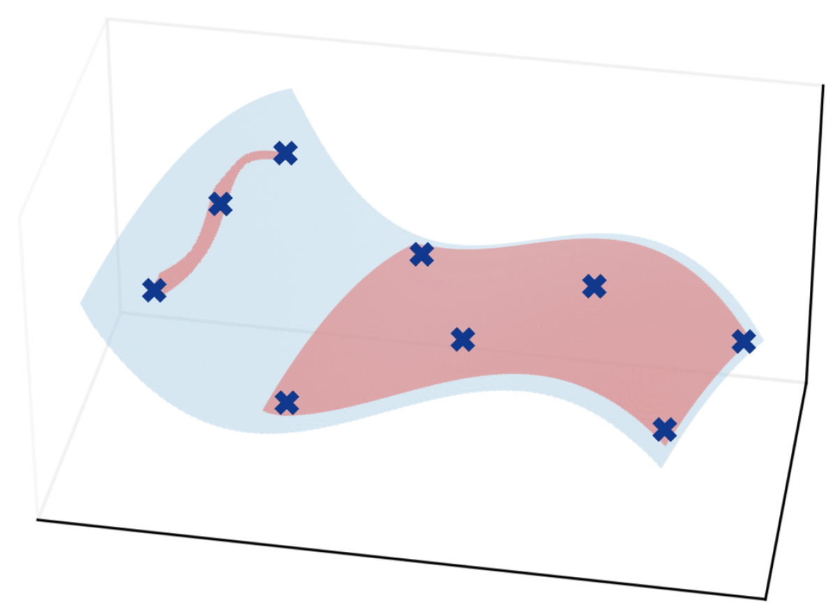
(b) OD-Mem with $\text{LID}_{\theta}(x)=1$

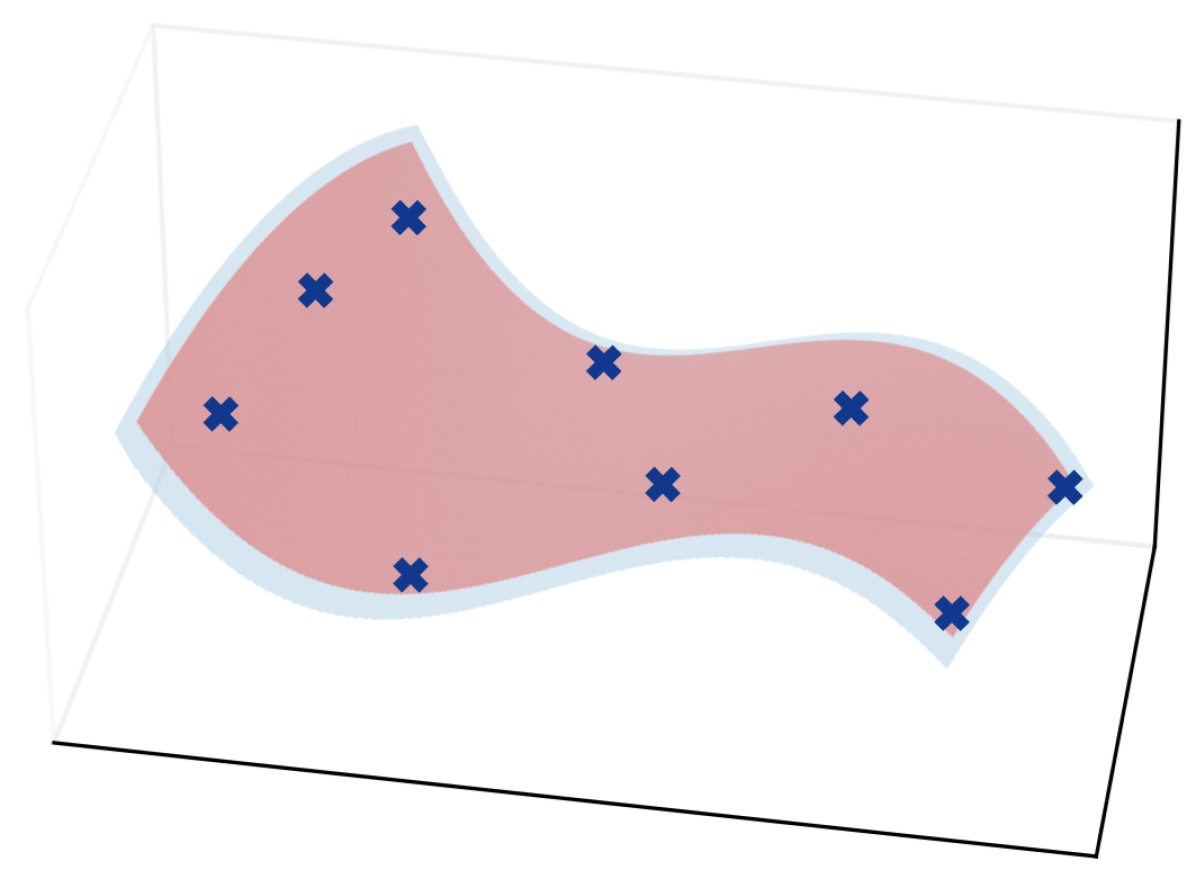
(c) No memorization with $\text{LID}_{\theta}(x)=2$

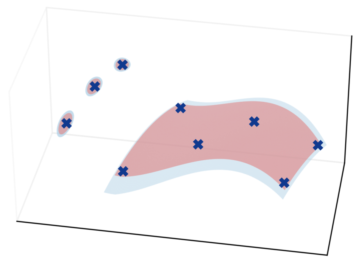
(d) DD-Mem with $\text{LID}_{\theta}(x)=0$

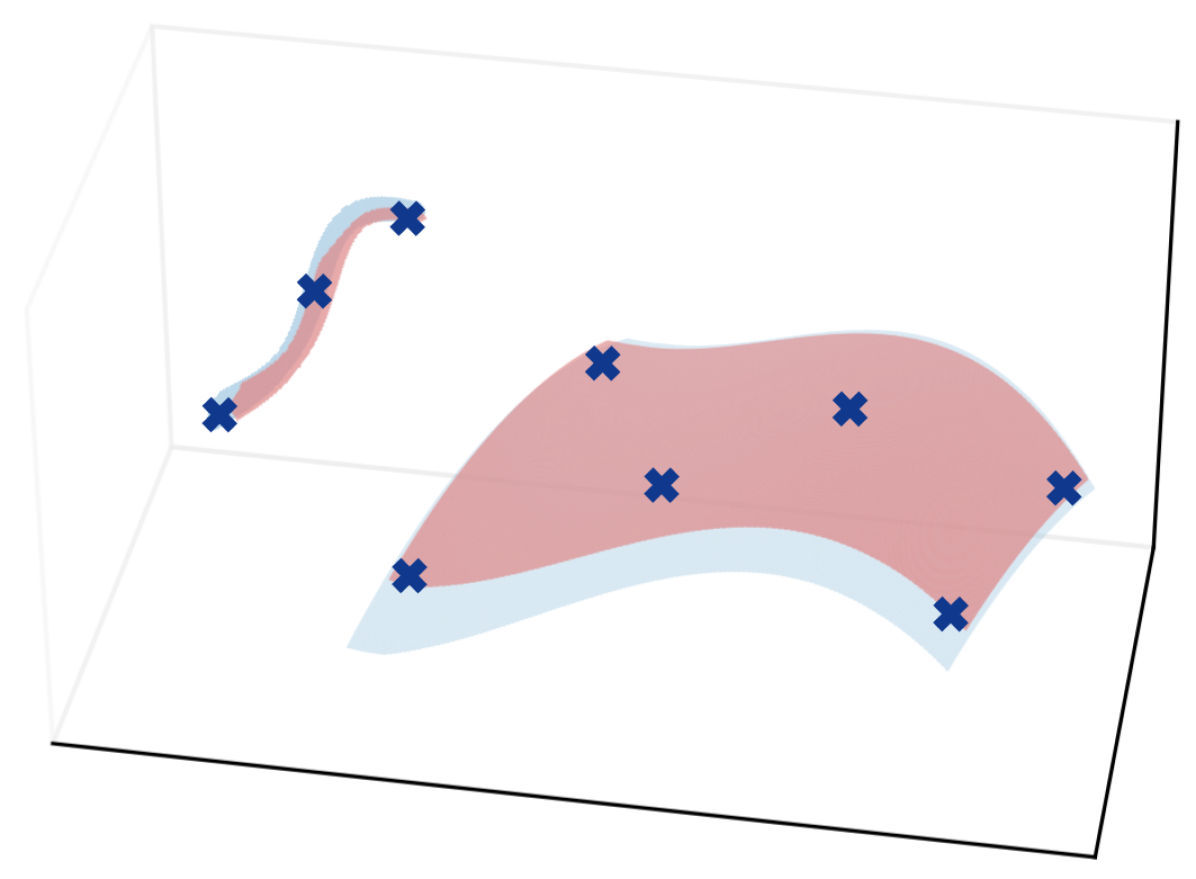
(e) DD-Mem with $\text{LID}_{\theta}(x)=1$

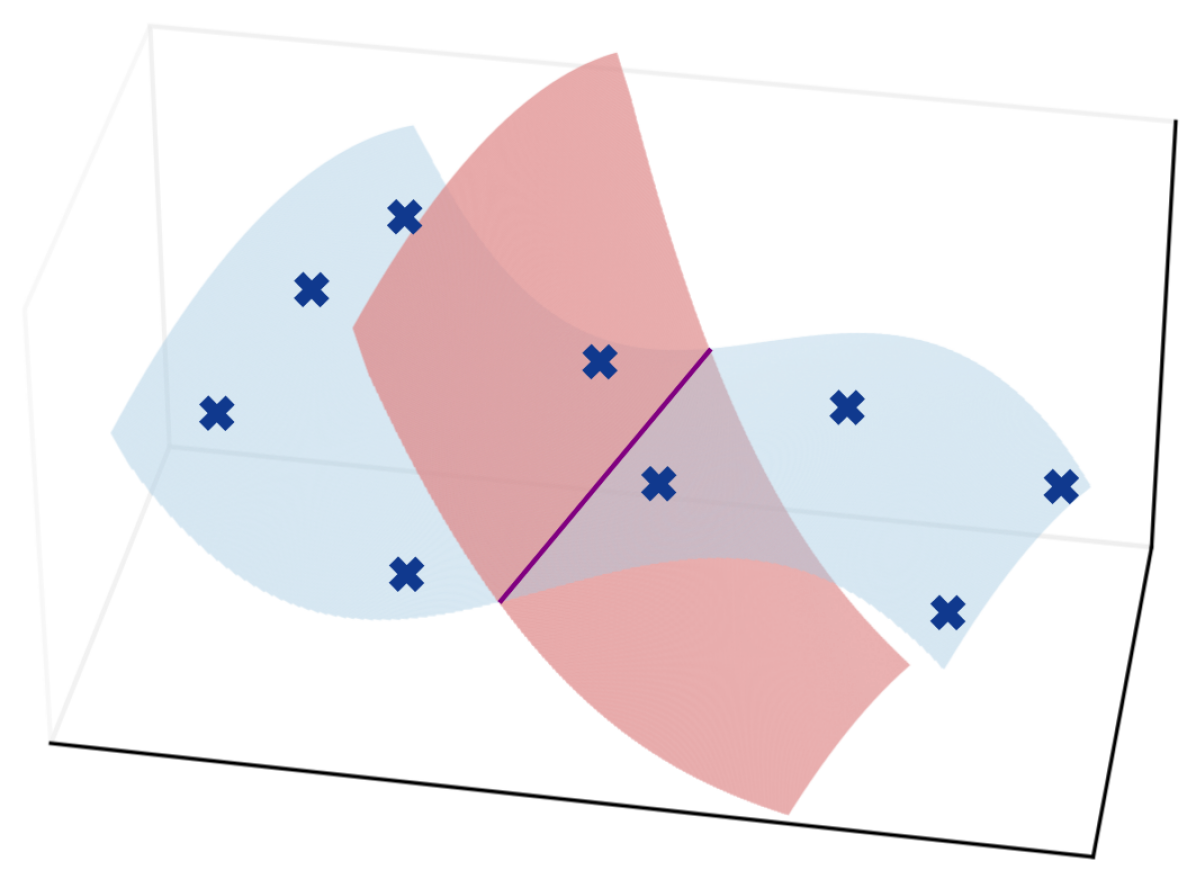
(f) Poorly fit model, LIDs are irrelevant

Figure 1: An illustrative example of LID values for models with different quality of fit and degrees of memorization. In these plots, the ground truth manifold $\mathcal{M}_{*}$ is depicted in light blue, training samples $\{x_{i}\}_{i=1}^{n}\subset\mathcal{M}_{*}$ are depicted as crosses, and the model manifolds $\mathcal{M}_{\theta}$ are depicted in red. In (a) and (d), the model assigns 0-dimensional point masses around the three leftmost datapoints, indicating that it will reproduce them directly at test time; however in the former case this is caused by overfitting ($\text{LID}_{\theta}(x)<\text{LID}_{*}(x)$), while in the latter it is caused by the ground truth data having small LID. The models in (b) and (e) are analoguous to (a) and (b), respectively, and still memorize, but with an extra degree of freedom in the form of a 1-dimensional submanifold containing the three points. Only the model in (c), which has learned a 2-dimensional manifold through its full support, has generalized well enough and has learned a manifold of high enough dimension to avoid both types of memorization. Finally, (f) shows a poorly fit model where LID and memorization are not meaningfully related.

Figure 2: 8 images along a relatively low-dimensional manifold learned by Stable Diffusion v1.5. The first is a real image from LAION (flagged as memorized by Webster (2023)), and the remainder were generated by the model.

The increasing dependence of society on generative models and resulting risks call for work to better understand memorization. Recent empirical work has identified mechanistic causes of memorization including but not limited to data complexity, duplication of training points, and highly specific labels (Somepalli et al., 2023b; Gu et al., 2023). We group these insights under the umbrella of “memorization phenomena”, a catch-all term for the various interesting memorization-related observations we would like to understand better. Though useful in practice, these memorization phenomena have yet to be unified and interpreted under a single theoretical framework. Meanwhile, formal treatments of memorization have led to isolated usecases such as detection (Meehan et al., 2020; Bhattacharjee et al., 2023) and prevention on a model level (Vyas et al., 2023), but have provided little explanatory power for memorization phenomena. In addition to providing theoretical insights, a unifying framework could yield more capabilities such as identifying whether a training image has been memorized, altering the sampling process to reduce memorization, and detecting memorized generations post hoc.

In this work, we introduce the manifold memorization hypothesis (MMH), a geometric framework to explain memorization. In short, we propose that memorization occurs at a point $x\in\mathbb{R}^{d}$ when the manifold learned by the generative model contains $x$ but has too small a dimensionality at $x$. As we will see, this understudied perspective is a natural take on memorization that leads to practical insights and effectively explains memorization phenomena like those mentioned above. Although we mainly focus on DMs, the most notorious memorizers, our geometric framework applies to any DGM on a continuous data space $\mathbb{R}^{d}$; indeed, we empirically validate it on generative adversarial networks (GANs; Goodfellow et al., 2014; Karras et al., 2019) as well. Pidstrigach (2022) was the first to show that DMs are capable of learning low-dimensional structure in $\mathbb{R}^{d}$ and that this manifold learning capability is a driver of memorization; in this sense, our work extends this connection into a general framework, grounds it in empirical findings, and connects it to recent work on memorization.

This paper is organized according to the following contributions.

1. We advance the MMH in Section 2. After defining the key notions of the data manifold and local intrinsic dimension (LID), we describe how LIDs correspond to memorization.

2. We demonstrate the explanatory power of the MMH in Section 3 by grounding it in prior observations about the behaviour of models that memorize. As this section will show, memorization phenomena observed in past work can be predicted and explained by the MMH.

3. In Subsection 4.1, we empirically test the MMH, showing that it both accurately describes reality and is useful in practice. As predicted by the MMH, estimates of LID are strongly predictive of memorization at scales ranging from 2-dimensional synthetic data to Stable Diffusion (Rombach et al., 2022).

4. Finally, inspired by the MMH, in Subsection 4.2 we devise scalable approaches to avert memorization during sampling from Stable Diffusion and to identify tokens in the text conditioning that contribute to memorization.

2 Understanding Memorization through LID

Preliminaries

Here we presume the manifold hypothesis: that data of interest lies on a manifold $\mathcal{M}\subset\mathbb{R}^{d}$ (Bengio et al., 2013). We take a generalized definition of manifold in which $\mathcal{M}$ is allowed to have different dimensionalities in different regions, which is appropriate for realistic, heterogeneous data with varying degrees of structure and complexity. In particular, we assume that both our ground truth distribution $p_{*}(x)$ and our model $p_{\theta}(x)$ produce samples on manifolds, which we refer to as $\mathcal{M}_{*}$ and $\mathcal{M}_{\theta}$ respectively. We direct readers to Loaiza-Ganem et al. (2024) for a justification and formal mathematical treatment of both of these assumptions, which are especially valid when the data is high-dimensional and the models are high-performing ones such as DMs and GANs.

Our framework for understanding memorization revolves around the notion of a point’s local intrinsic dimension (LID). Given a manifold $\mathcal{M}$ and a point $x\in\mathcal{M}$, we define the LID of $x$, $\text{LID}(x)$, with respect to $\mathcal{M}$ as the dimensionality of $\mathcal{M}$ at $x$. In this work, we will mainly consider the LIDs of points $x\in\mathbb{R}^{d}$ with respect to two specific manifolds: $\mathcal{M}_{*}$ and $\mathcal{M}_{\theta}$. We will refer to these quantities as $\text{LID}_{*}(x)$ and $\text{LID}_{\theta}(x)$, respectively.

Intuition and the Manifold Hypothesis Before discussing our framework, we review some intuition relating the manifold hypothesis to practical datasets. Manifold structure $\mathcal{M}\subset\mathbb{R}^{d}$ arises from sets of constraints. These can range from very simple, like a set of linear constraints ($\mathcal{M}=\{x\mid Ax=b\}$), to highly complex ($\mathcal{M}=\{x\mid x\text{ is an image of a face}\}$). Locally at a point $x\in\mathcal{M}$, each constraint determines a direction one cannot move without leaving the manifold and violating the structure of the dataset. Hence, a region governed by $\ell$ independent and active constraints will have dimensionality $\text{LID}(x)=d-\ell$. The value of $\text{LID}(x)$ represents the number of degrees of freedom – valid directions of movement in which the characteristics of the dataset are preserved. Another connection is to complexity. For example, estimates of LID from algorithms like FLIPD (Kamkari et al., 2024b) or the normal bundle (NB) method of Stanczuk et al. (2024) (which we use in our experiments; see Appendix B for details) have been shown to correspond closely with the complexity of an image; it is reasonable to expect that images with more complex features can endure more changes (such as morphing, moving, or changing the colours of different parts of the image) without losing coherence. The notions of constraints, degrees of freedom, and complexity along with their relationship to LID will help us understand its connection to memorization in later sections.

A Geometric Framework for Understanding Memorization In this section we formulate a framework for understanding memorization based on comparisons between $\text{LID}_{\theta}(x)$ and $\text{LID}_{*}(x)$. As a motivating example, consider Figure 1, which depicts six possible models $p_{\theta}(x)$ trained on datasets $\{x_{i}\}_{i=1}^{n}$ that each lie on a ground truth manifold $\mathcal{M}_{*}$. In the first scenario, 1(a), the model $p_{\theta}(x)$ has precisely memorized some of the training data. This is a well-understood mode of memorization; training datapoints are exactly reproduced. To achieve this, the model has learned a 0-dimensional manifold around these datapoints. To our knowledge, Pidstrigach (2022) was the first to point out that a model capable of learning 0-dimensional manifolds can memorize the training data. From this example, we infer that $x$ can be perfectly reproduced when $\text{LID}_{\theta}(x)=0$. This indicates suboptimality in the model at the datapoints shown, for which $\text{LID}_{*}(x)=2$.

However, memorization can be more complex than simply reproducing a datapoint. For example, Somepalli et al. (2023a) identify instances where layouts, styles, or foreground or background objects in training images are copied without copying the entire image, a phenomenon they refer to as reconstructive memory. Webster (2023) surfaces more instances of the same phenomenon and refers to them as template verbatims. See Figure 2 for an example. In the region of these points $x\in\mathcal{M}_{\theta}$, the model is able to generate images with degrees of freedom in some attributes (e.g., colour or texture), but is too constrained in other attributes (e.g., layout, style, or content). Geometrically, $\mathcal{M}_{\theta}$ is too constrained compared to the idealized ground truth manifold $\mathcal{M}_{*}$; i.e., $\text{LID}_{\theta}(x)<\text{LID}_{*}(x)$. We depict this situation in 1(b), wherein the model has erroneously assigned $\text{LID}_{\theta}(x)=1$ for some of the training datapoints.

Two Types of Memorization We expect two types of memorization to be of interest. An academic interested in designing DGMs that learn the ground truth distribution correctly will chiefly be interested in avoiding the memorization scenario $\text{LID}_{\theta}(x)<\text{LID}_{*}(x)$. We refer to this first scenario as overfitting-driven memorization (OD-Mem). This situation represents a modelling failure in that $p_{\theta}(x)$ is not generalizing correctly to $p_{*}(x)$, and is illustrated in 1(a) and 1(b).

However, an industry practitioner deploying a consumer-facing model might be more interested in hypothetical values of $\text{LID}_{\theta}$ per se, irrespective of the values of $\text{LID}_{*}$. For any points $x\in\mathcal{M}_{*}$ containing trademarked or private information, low values of $\text{LID}_{\theta}(x)$ will be of concern even if $\text{LID}_{\theta}(x)=\text{LID}_{*}(x)$, as this information is likely to be revealed in samples generated from this region. A practitioner would rightly refer to this situation as memorization despite the model generalizing correctly. We refer to this second scenario as data-driven memorization (DD-Mem), and illustrate it in 1(d) and 1(e). This certainly happens in practice; for example, conditioning on the title of a specific artwork (e.g. “The Great Wave off Kanagawa” by Katsushika Hokusai (Somepalli et al., 2023a)) is a very strong constraint, leaving few degrees of freedom in the ground truth manifold $\mathcal{M}_{*}$, but reproducing specific artworks may be undesirable in a production model. Unlike OD-Mem, DD-Mem is not overfitting in the classical sense, and a notable consequence is that it cannot be detected by comparing training and test likelihoods. We refer to the conceptualization of how LIDs relate to memorization through OD-Mem and DD-Mem as the manifold memorization hypothesis.

No memorization is present in 1(c), in which the model manifold $\mathcal{M}_{\theta}$ matches the desired ground truth manifold $\mathcal{M}_{*}$. We highlight that the MMH assumes high-performing models whose manifold $\mathcal{M}_{\theta}$ is roughly aligned with the data manifold $\mathcal{M}_{*}$; when this is not the case, as in 1(f), $\text{LID}_{\theta}$ and its relationship to $\text{LID}_{*}$ become irrelevant to memorization.

Why is the MMH Useful?

The MMH is a hypothesis about how memorization occurs in practice for high-dimensional data. Its utility is best framed in contrast to past treatments of memorization. First, while past theoretical frameworks for memorization have focused on probability mass, our geometric perspective leads to more practical tools. For example, Bhattacharjee et al. (2023) propose a purely probabilistic definition of memorization that can be detected only with access to the training dataset and the ability to generate large numbers of samples, which are intractable requirements at the scale of LAION-2B (Schuhmann et al., 2022) and Stable Diffusion. In contrast, the MMH suggests that memorization can be detected through $\text{LID}_{\theta}(x)$, for which tractable estimators exist at scale. We explore these estimators in Section 4.

Second, the MMH distinguishes between OD-Mem and DD-Mem, while past analyses have not. Bhattacharjee et al. (2023) would allow for OD-Mem but not DD-Mem under its definition of memorization, while empirical work tends to ignore the effect of $p_{*}(x)$ on $p_{\theta}(x)$, thus subsuming both OD-Mem and DD-Mem in spirit if not formally (Carlini et al., 2023; Yoon et al., 2023; Gu et al., 2023). For further details, please see Appendix A, where we formally develop the relationship between the MMH and definitions of memorization in related work.

Defining and distinguishing between OD-Mem and DD-Mem suggests immediate solutions to each. DD-Mem indicates that the training distribution $p_{*}(x)$ does not actually match the desired distribution at inference time, and hence is a misalignment of data and objectives. It can be addressed by changing $p_{*}(x)$ itself, such as by altering the data collection, cleaning, and augmentation procedures. We explore this point further in Section 3. Unlike OD-Mem, DD-Mem cannot be addressed by improving the model to have better generalization. Both OD-Mem and DD-Mem can also in principle be addressed by augmenting $p_{\theta}(x)$ to generate higher-LID samples. In Section 4, we propose solutions to alter the data-generating process with precisely this goal.

3 Explaining Memorization Phenomena

In this section, we demonstrate the explanatory power of the MMH by showing how it explains memorization phenomena in related work. In the process, this section demonstrates two advantages of our geometric framework. First, it provides a unifying perspective on seemingly disparate observations throughout the literature (nevertheless, this is not meant as a related work section — for that see Section 5). Second, it links memorization to the rich theoretical toolboxes of measure theory and geometry, which we use in this section to establish formal connections to past work. Propositions, theorems, and proofs in this section are presented informally for clarity. For full theorem statements and proofs, please see Appendix E.

Duplicated Data and LID It has been broadly observed that memorization occurs when training points are duplicated (Nichol et al., 2022; Carlini et al., 2022; Somepalli et al., 2023a). In 3.1, we show that duplicated datapoints lead to DD-Mem; duplicated points $x_{0}$ indicate $\text{LID}_{*}(x_{0})=0$, so even a correctly fitted model will have $\text{LID}_{\theta}(x_{0})=0$ (as in 1(d)).

Proposition 3.1 (Informal).

Let $\{x_{i}\}_{i=1}^{n}$ be a training dataset drawn independently from $p_{*}(x)$. Under some regularity conditions, the following hold:

1. If duplicates occur in $\{x_{i}\}_{i=1}^{n}$ with positive probability, then they occur at a point $x_{0}$ such that $\text{LID}_{*}(x_{0})=0$.

2. If $\text{LID}_{*}(x_{0})=0$ and $n$ is sufficiently large, then duplication will occur in $\{x_{i}\}_{i=1}^{n}$ with near-certainty.

Proof.

See Appendix E for the formal statement of the theorem and proof. To understand both conditions intuitively, it suffices to note first that duplicate samples are intuitively equivalent to $P_{*}$ assigning positive probability to a point. Under mild regularity conditions on the nature of the $p_{*}(x)$ and $\mathcal{M}_{*}$, positive probability at a point is equivalent to a 0-dimensional manifold at that point. ∎

From this result, we gather that improving model generalization is not the solution to duplication. Instead, one may need to add inductive biases that prevent $p_{\theta}(x)$ from learning 0-dimensional points. Of course, the more straightforward path is to change the data distribution $p_{*}(x)$ by de-duplicating the training dataset. We carry the same intuition forward to “near-duplicated content”, where similar but non-identical points occur together in the dataset, in which case $\text{LID}_{*}$ would be low but nonzero in the region of the near-duplicated content (as in 1(e)).

Conditioning and LID  Somepalli et al. (2023b) and Yoon et al. (2023) observe that conditioning on highly specific prompts $c$ encourages the generation of memorized samples. Here, we point out that conditioning decreases LID, making models more likely to generate memorized samples.

Proposition 3.2 (Informal).

Let $x_{0}\in\mathcal{M}_{*}$, and let us denote by $\text{LID}_{*}(x_{0}\mid c)$ the LID of $x_{0}$ with respect to the support of the conditional distribution $p_{*}(x\mid c)$. We then have

$$\text{LID}_{*}(x_{0}\mid c)\leq\text{LID}_{*}(x_{0}).$$ (1)

Proof.

See Appendix E for the formal statement of the theorem and proof. Intuitively, conditioning can be interpreted as adding additional constraints to $\mathcal{M}_{*}$, which cannot increase its dimension. ∎

Conditioning on highly specific $c$ can be linked to both DD-Mem and OD-Mem. Introducing strong constraints greatly decreases $\text{LID}_{*}$, leading to DD-Mem. However, if a relatively low number of training examples satisfy $c$, the model could overfit, leading to OD-Mem as well.

Complexity and LID For images, Somepalli et al. (2023b) also highlight low complexity as a factor causing memorization. Using the understanding that LID corresponds to complexity as discussed in Section 2, we infer that low-complexity datapoints $x\in\mathcal{M}_{*}$ have low $\text{LID}_{*}(x)$. This fact suggests that, like with duplication, memorization of low-complexity datapoints is an example of DD-Mem.

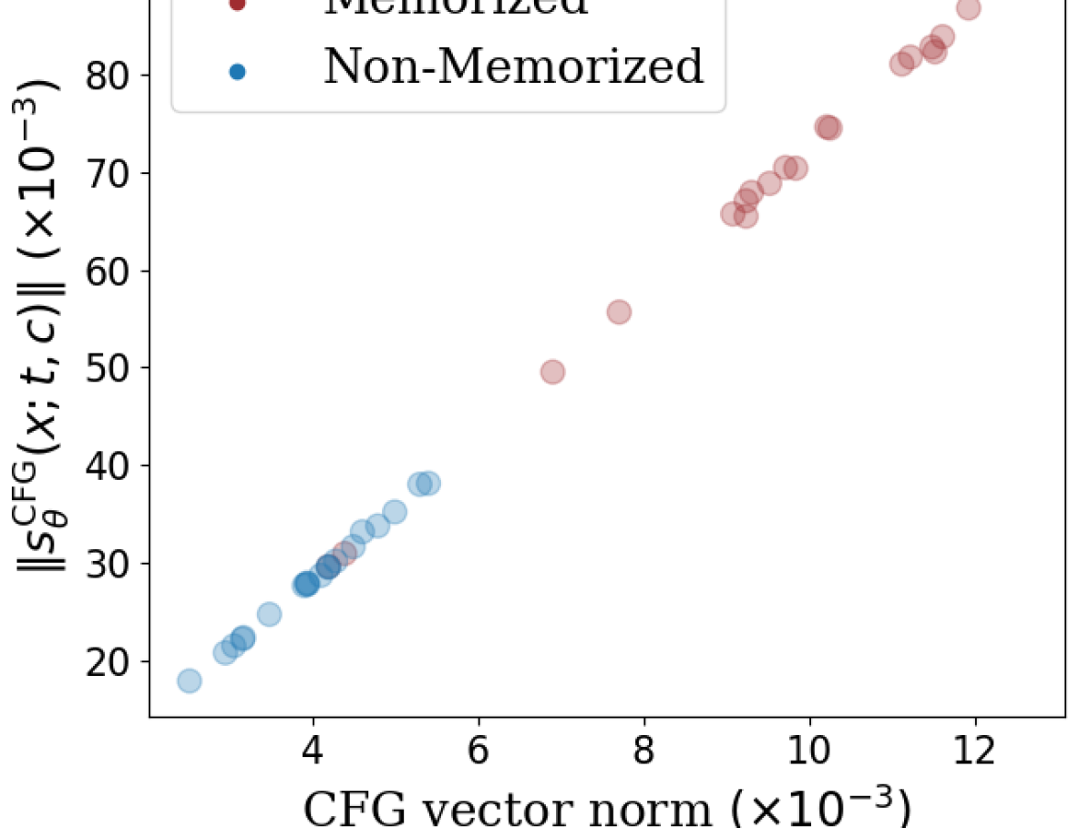
Figure 3: CFG-adjusted scores vs CFG vectors for Stable Diffusion with $\lambda=7.5$ and $t=0.02$ on $20$ memorized and $20$ non-memorized images from LAION.

The Classifier-Free Guidance Norm and LID  Classifier-free guidance (CFG) is a way to improve the quality of conditional generation. Whereas standard conditional generation employs the score function $s_{\theta}(x;t,c)$, which refers to a neural estimate at time $t$ of the conditional score, CFG increases the strength of conditioning by using the following modified score:

where $\lambda$ is a hyperparameter for “guidance strength” and $s_{\theta}(x;t,\emptyset)$ refers to conditioning on the empty string (here we formulate DMs using stochastic differential equations (Song et al., 2021)).

Wen et al. (2023) identify that specific conditioning inputs $c$ lead to memorized samples when the CFG vector has a large magnitude. We explain this observation using the MMH as follows. First, we observe that a large CFG magnitude will generally result in a large magnitude of the CFG-adjusted score $s^{\text{CFG}}_{\theta}(x;t,c)$. We demonstrate this empirically in Figure 3. Furthermore, it is understood in the literature that a large $\lVert s^{\text{CFG}}_{\theta}(x;t,c)\rVert$, and its explosion as $t\to 0$, is common for high-dimensional data (Vahdat et al., 2021) and is necessary to generate samples from low-dimensional manifolds (Pidstrigach, 2022; Lu et al., 2023). It has been empirically observed that this explosion occurs faster as the dimensionality gap increases between the data manifold and the ambient data space (Loaiza-Ganem et al., 2024), which is one reason that generative modelling on lower-dimensional latent space tends to improves performance (Loaiza-Ganem et al., 2022). The largest $\lVert s^{\text{CFG}}_{\theta}(x;t,c)\rVert$ values should thus generate points with the largest dimensionality difference from $\mathbb{R}^{d}$; i.e., points $x$ with the smallest $\text{LID}_{\theta}(x\mid c)$. Hence we infer that reducing the CFG-adjusted score norm – or equivalently the CFG vector norm – should increase $\text{LID}_{\theta}(x\mid c)$ and lessen memorization, a fact confirmed empirically by Wen et al. (2023). Since this phenomenon corresponds to any $x$ with small $\text{LID}_{\theta}(x\mid c)$, it can indicate both OD-Mem and DD-Mem under the MMH.

4 Experiments

4.1 Verifying the Manifold Memorization Hypothesis

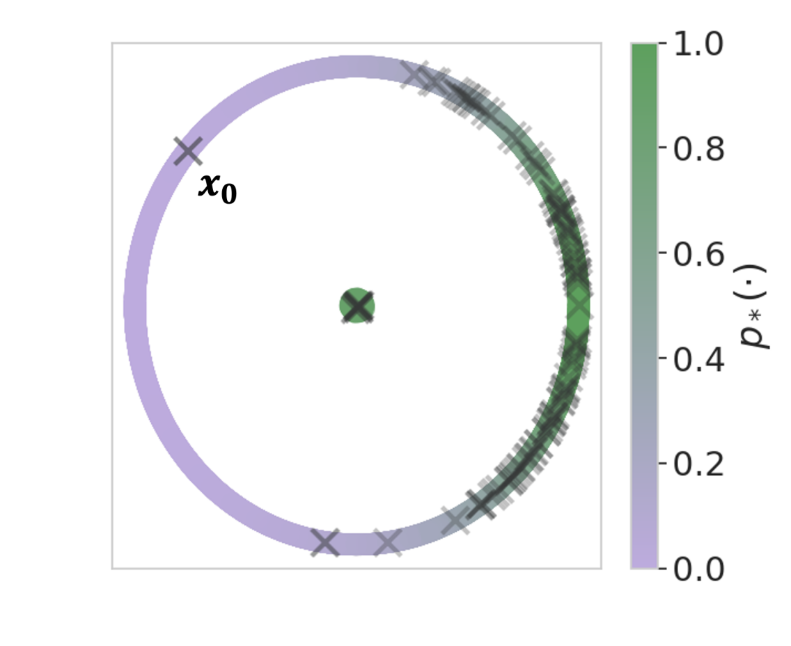
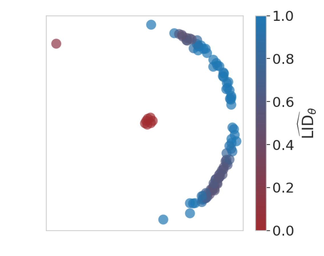
Figure 4: Training a diffusion model on a von Mises mixture. (Top) Ground truth manifold and the associated distribution. (Bottom) Model-generated samples with their LID estimates.

In this section, we empirically verify the geometric framework which underpins the MMH. We analyze both $\text{LID}_{*}$ and $\text{LID}_{\theta}$ to study DD-Mem and OD-Mem. Several algorithms exist to estimate $\text{LID}_{\theta}(x)$ for diffusion models, including the normal bundle (NB) method (Stanczuk et al., 2024), and more recently FLIPD (Kamkari et al., 2024b). For GANs, we approximate $\text{LID}_{\theta}(x)$ of generated data by computing the rank of the Jacobian of the generator. Additionally, we use LPCA (Fukunaga & Olsen, 1971) to estimate $\text{LID}_{*}$ where applicable; see Appendix B for details on these methods and Appendix C for their hyperparameter configurations. In general $\text{LID}_{\theta}$ and $\text{LID}_{*}$ are unknown quantities that are approximated with the aforementioned estimators, throughout this section we write their respective estimates as $\widehat{\text{LID}}_{\theta}$ and $\widehat{\text{LID}}_{*}$.

Diffusion Model on a von Mises Mixture In an illustrative experiment, we study a mixture of a von Mises distribution, which sits on a 1-dimensional circle, and a 0-dimensional point mass at the origin in 2-dimensional ambient space, as depicted in Figure 4; every point $x$ has either $\text{LID}_{*}(x)=0$ or $\text{LID}_{*}(x)=1$. From this distribution we sample 100 training points, and by chance a single point $x_{0}$ sits isolated in a low-density region of the circle. Next, we train a DM on this data. In Figure 4 we depict 100 generated samples, colour-coded by their LID estimates, as estimated by FLIPD. Here, we see OD-Mem and DD-Mem in action: the model overfits at $x_{0}$, producing near-exact copies, with $0\approx\widehat{\text{LID}}_{\theta}(x_{0})<\text{LID}_{*}(x_{0})=1$ (OD-Mem). The model faithfully produces copies of the circle’s center too, yet this is not caused by a modelling error but by the low associated LIDs (DD-Mem).

IFAR10 Memorization We analyze the higher-dimensional CIFAR10 dataset (Krizhevsky & Hinton, 2009) and use two pre-trained generative models: iDDPM (Nichol & Dhariwal, 2021) and StyleGAN2-ADA (Karras et al., 2020). We generate 50,000 images from each model. Since StyleGAN2-ADA is class-conditioned, we generate an equal number of samples per class. We then retrieve $500$ images from the dataset using both $(i)$ SSCD distance (Pizzi et al., 2022) and $(ii)$ calibrated $\ell_{2}$ distance (Carlini et al., 2023). We take the top $250$ returned from each ranking, producing a set of just under $500$ images we can visually examine. We then label all of these instances as either not memorized, exactly memorized, or reconstructively memorized (Somepalli et al., 2023a). Images not appearing in the top $250$ of either ranking are not labelled, and have a low chance of being memorized. The first two panels in 5(a) show our labels distinguish different types of memorization as we display the generated images vs. the closest SSCD match in the training dataset.

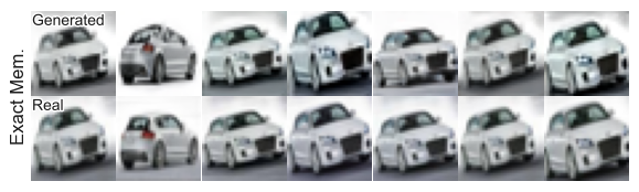
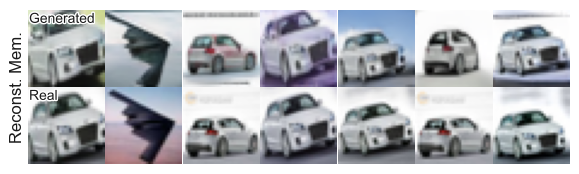
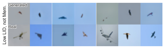
(a) (Left) Exact and (Middle) reconstructively memorized samples (Top) with their matched CIFAR10 datapoints (Bottom). (Right) Non-memorized samples with low $\widehat{\text{LID}}_{\theta}$, showing $\widehat{\text{LID}}_{\theta}$ can be partially confounded by complexity.

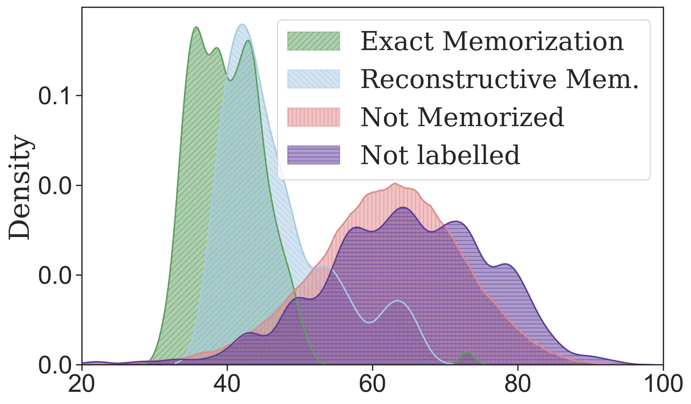
(b) $\widehat{\text{LID}}_{\theta}$ for StyleGAN samples.

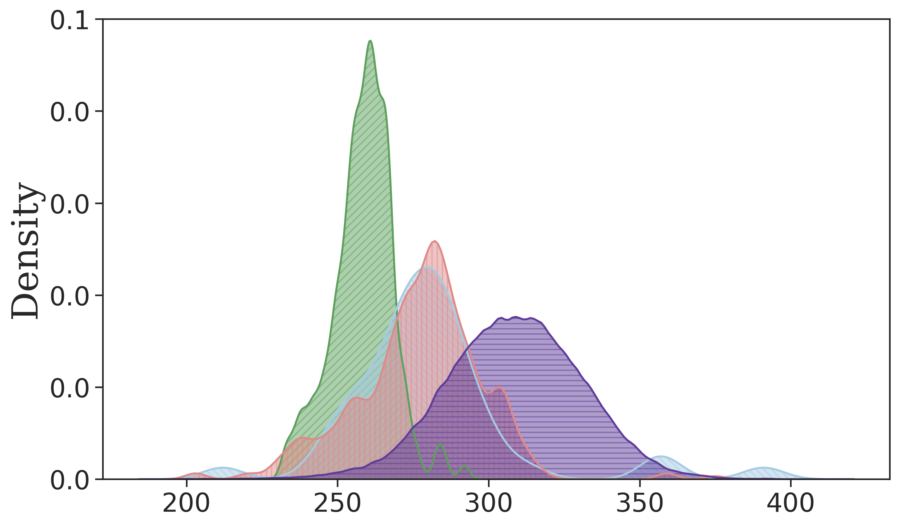
(c) $\widehat{\text{LID}}_{\theta}$ for iDDPM samples.

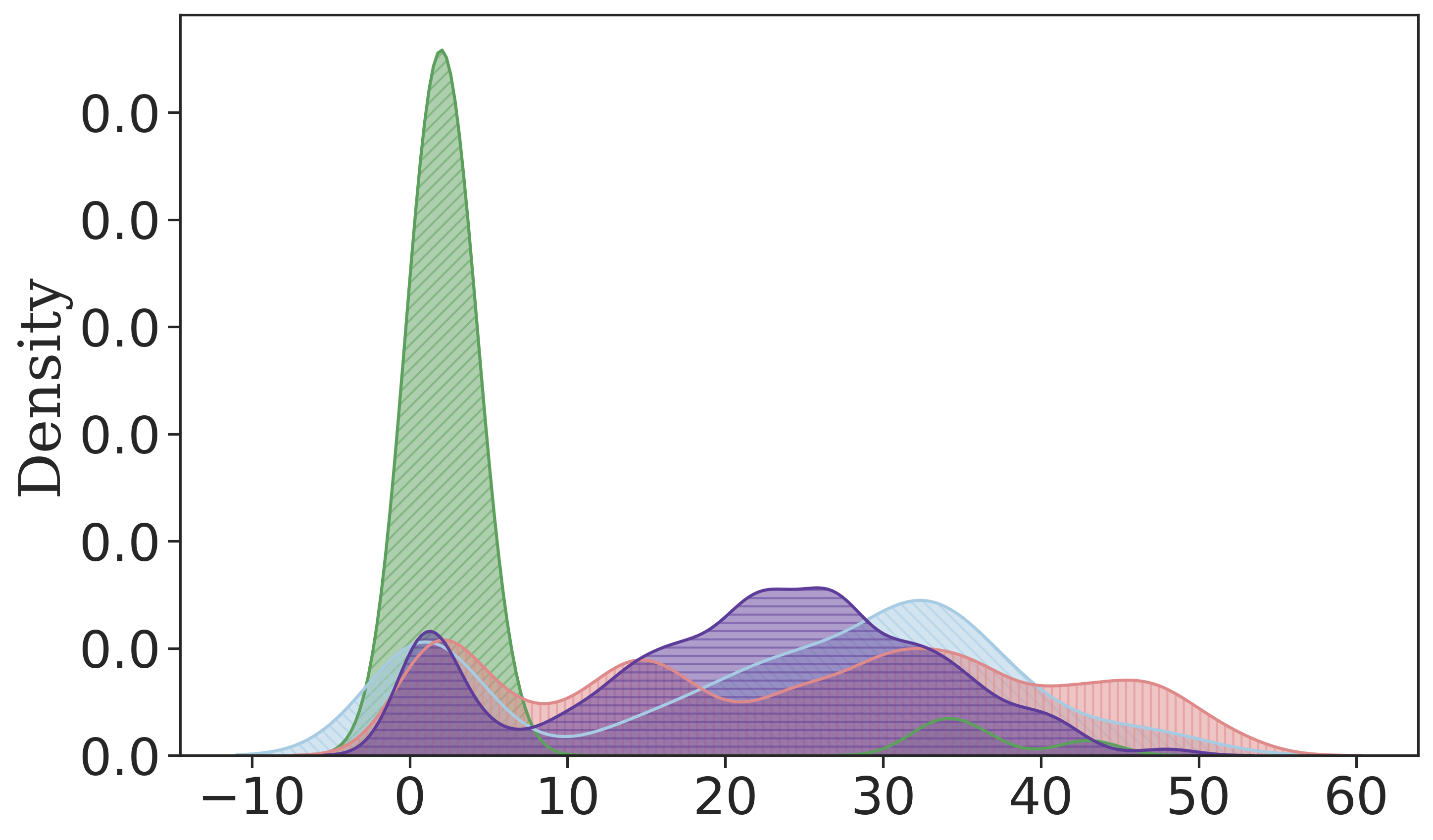
(d) $\widehat{\text{LID}}_{*}$ for CIFAR10 datapoints.

Figure 5: Visualizing OD-Mem and DD-Mem on StyleGAN2-ADA and iDDPM trained on CIFAR10.

Next, we estimate $\text{LID}_{\theta}$ for each iDDPM and StyleGAN2-ADA sample. For iDDPM, we use the NB estimator. 5(b) and 5(c) show that $\widehat{\text{LID}}_{\theta}$ is generally smaller for memorized images compared to non-memorized ones. As shown in 5(d), $\widehat{\text{LID}}_{*}$ is considerably lower for exact memorization cases within the training dataset, suggesting that exact memorization for both models corresponds to DD-Mem. We also observe that in 5(b), reconstructively memorized samples exhibit lower values of $\widehat{\text{LID}}_{\theta}$ as compared to not memorized samples, despite the corresponding training data having comparable $\widehat{\text{LID}}_{*}$ (5(d)): the $\text{LID}_{\theta}$ estimates enable us to still classify these samples as memorized, showing a clear example of detecting OD-Mem.

We have shown that LID estimates are effective at detecting both OD-Mem and DD-Mem, supporting the MMH hypothesis. However, while simpler images tend to be memorized more frequently, they are not always memorized (see 5(a), right panel), leading to some overlap in estimated $\text{LID}_{\theta}$ between memorized and not memorized samples in 5(b) and 5(c). This overlap occurs because image complexity serves as a confounding factor: images with simple backgrounds and textures may be assigned low $\text{LID}_{\theta}$ values, not due to memorization, but simply because of their inherent simplicity. We discuss this issue further, along with a partial solution, in Appendix C.2.

Stable Diffusion on Large-Scale Image Datasets Here, we set $p_{\theta}(x)$ to Stable Diffusion v1.5 (Rombach et al., 2022). Taking inspiration from the benchmark of Wen et al. (2023), we retrieve memorized LAION (Schuhmann et al., 2022) training images identified by Webster (2023). We focus on the 86 memorized images categorized as “matching verbatim”, noting that the other categories of Webster (2023) consist of large numbers of captions that generate samples matching a small set of training images. For non-memorized images, we use a mix of 2000 images sampled from LAION Aesthetics 6.5+, 2000 sampled from COCO (Lin et al., 2014), and all 251 images from the Tuxemon dataset (Tuxemon Project, 2024; Hugging Face, 2024).

To our knowledge, no estimator of $\text{LID}_{*}$ scales to images at the size of Stable Diffusion; we thus omit these from our analysis. FLIPD is the only $\text{LID}_{\theta}$ estimator that remains tractable at this scale, so we use it for this analysis. Note that Stable Diffusion provides two model distributions: the unconditional distribution $p_{\theta}(x)$ and the conditional distribution $p_{\theta}(x\mid c)$, where $c$ is the image’s caption. Hence, we compute both $\widehat{\text{LID}}_{\theta}$ and $\widehat{\text{LID}}_{\theta}(\cdot\mid c)$ for each of the aforementioned images. The density histograms of all these values are depicted in Figure 6. We see that both $\widehat{\text{LID}}_{\theta}$ and $\widehat{\text{LID}}_{\theta}(\cdot\mid c)$ are relatively smaller for memorized images, further supporting the MMH. Due to the unavailability of $\text{LID}_{*}$ estimates, it is hard to distinguish between DD-Mem and OD-Mem here.

We also compare to a method by Wen et al. (2023), where the norm of the CFG vector is used to detect memorization (see Appendix C for details). In Figure 6, low conditional or unconditional LID as well as high CFG vector norms are all signals of memorization, strengthening our argument in Section 3. While the CFG vector norm seemingly provides the strongest signal, the unconditional LID detects memorization well despite the lack of caption information. Detecting memorized training images without the corresponding captions is a novel capability, and notably cannot be done with the CFG vector norm technique.

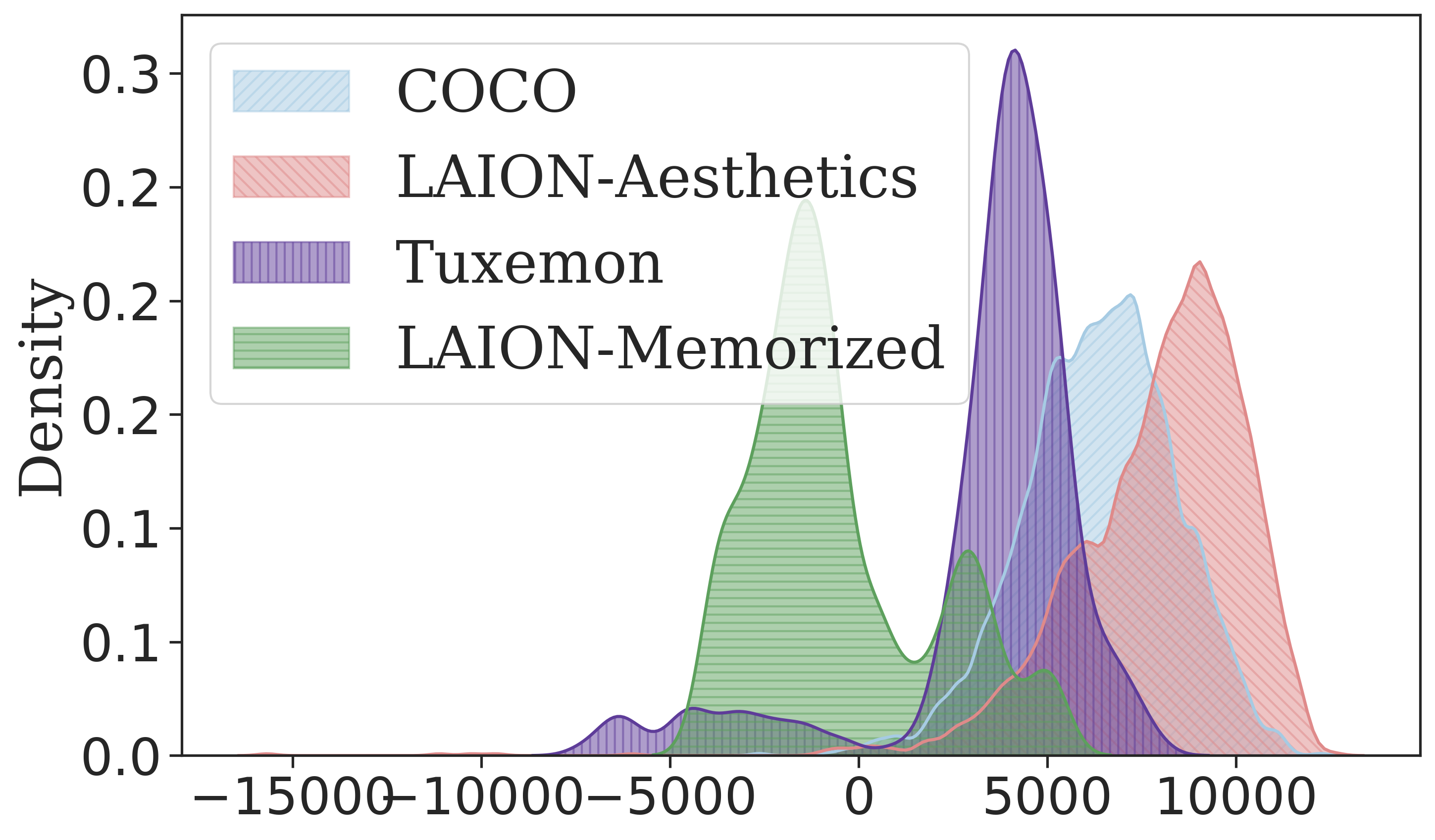
(a) $\widehat{\text{LID}}_{\theta}$.

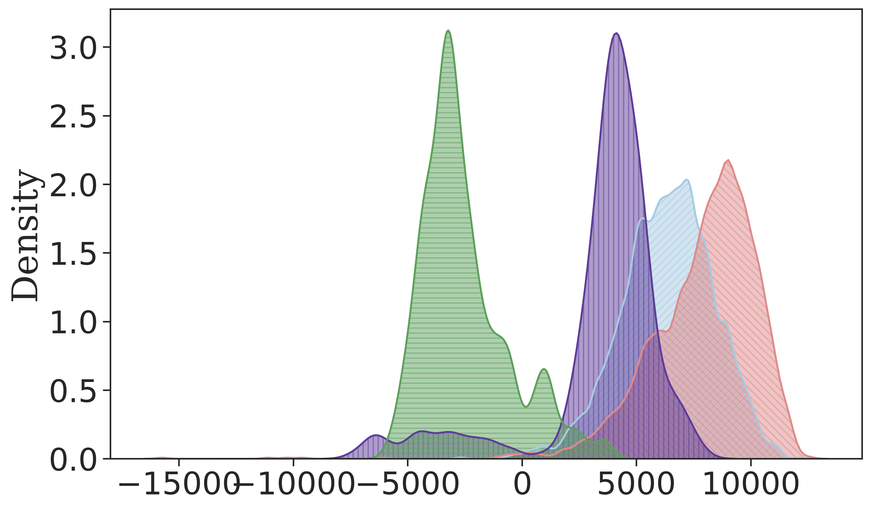
(b) $\widehat{\text{LID}}_{\theta}(\cdot\mid c)$.

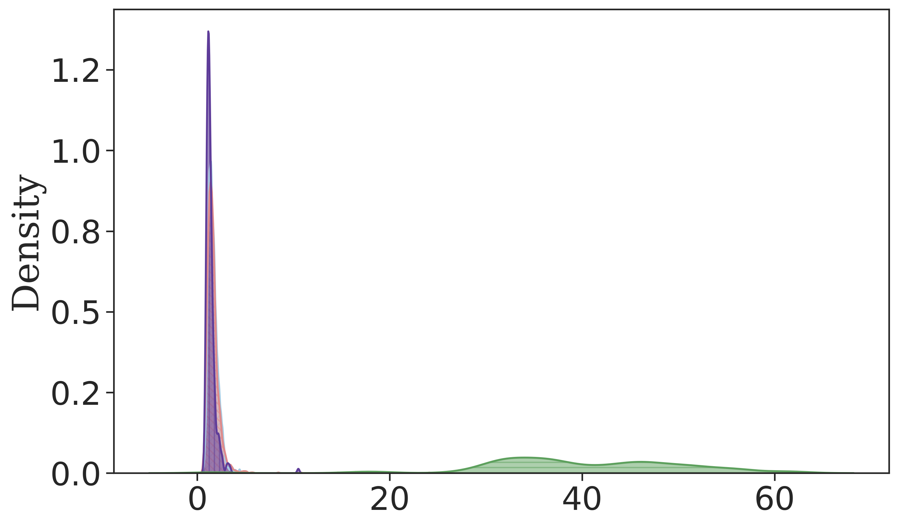
(c) CFG vector norm.

Figure 6: Density histograms for each memorization metric across different datasets.

4.2 Mitigating Memorization by Controlling $\text{LID}_{\theta}$

In this section we study the problem of sample-time mitigation through the lens of the MMH. Somepalli et al. (2023b) establish text-conditioning as a crucial driver of memorization in Stable Diffusion, where specific tokens in the prompt often cause the model to generate replicas of training images. Wen et al. (2023) introduce a differentiable metric, which we denote as $\mathcal{A}^{\text{CFG}}(c)$ (formally defined in Appendix D), which is based on the accumulated CFG vector norm while sampling an image. Wen et al. (2023) observe that this metric shows a sharp increase when the prompt $c$ leads to the generation of memorized images. Since $\mathcal{A}^{\text{CFG}}(c)$ is differentiable with respect to $c$, Wen et al. (2023) backpropagate through this metric and find the tokens with the largest gradient magnitude, essentially providing token attributions for memorization.

Here we make two contributions. First, we propose two additional metrics, $\mathcal{A}^{s_{\theta}^{\text{CFG}}}(c)$ and $\mathcal{A}^{\text{FLIPD}}(c)$, which are modifications of $\mathcal{A}^{\text{CFG}}(c)$ to use $\|s^{\text{CFG}}_{\theta}(x;t,c)\|$ or FLIPD respectively instead of the norm of the CFG vector. We define these metrics fully in Appendix D due to space limitations. Since both of these new metrics are also differentiable with respect to $c$, $\mathcal{A}^{\text{CFG}}(c)$ can be trivially replaced by either of them in the method of Wen et al. (2023). Second, we propose an automated way to use the token attributions from this method into a sample-time mitigation scheme. We start by normalizing the attributions across the tokens, and sample $k$ tokens based on a categorical distribution parameterized by these normalized attributions. We then use GPT-4 (OpenAI, 2023) to rephrase the caption, keeping it semantically similar but perturbing the selected $k$ tokens that are highly contributing to the memorization metric (see Appendix D.4 for details).

The bottom panel in 7(b) shows four images: a training image corresponding to the prompt “The Great Wave off Kanagawa by Katsushika Hokusai”, a generated image using the same prompt showing clear memorization, a generated image obtained with our mitigation scheme with $\mathcal{A}^{\text{CFG}}(c)$, and another generated image using $\mathcal{A}^{\text{FLIPD}}(c)$ instead. Qualitatively, using FLIPD or the norm of the CFG vector perform on par with each other. The top panel of 7(b) shows the token attributions obtained from $\mathcal{A}^{\text{FLIPD}}(c)$ are sensible. See Appendix D.5 for additional results.

We present quantitative comparisons in 7(a) by analyzing the average CLIP score (Radford et al., 2021) and SSCD similarity over matching prompts, varying $k\in\{1,2,3,4,6,8\}$, with $5$ repetitions for each prompt. As $k$ increases, both similarity score (lower is better) and CLIP score (higher is better) consistently decrease across methods. We include an additional baseline where the modified tokens are selected uniformly at random, ignoring attributions. All attribution-based methods achieve lower similarity while maintaining a relatively higher CLIP score than the random baseline.

Overall, the results in Figure 7 provide further evidence supporting the MMH, both by showing that encouraging samples to have higher LID can help prevent memorization, and by further confirming the relationship between the CFG vector norm, the CFG-adjusted score norm, and LID established in Section 3. We hypothesize that our results can likely be improved by more efficiently guiding generated samples towards regions of high LID, but highlight that doing so is not trivial. For example, in Appendix D.3 we find that using guidance towards large values of $\mathcal{A}^{\text{FLIPD}}(c)$ during sampling can fail by producing samples with chaotic textures that have artificially high $\text{LID}_{\theta}$.

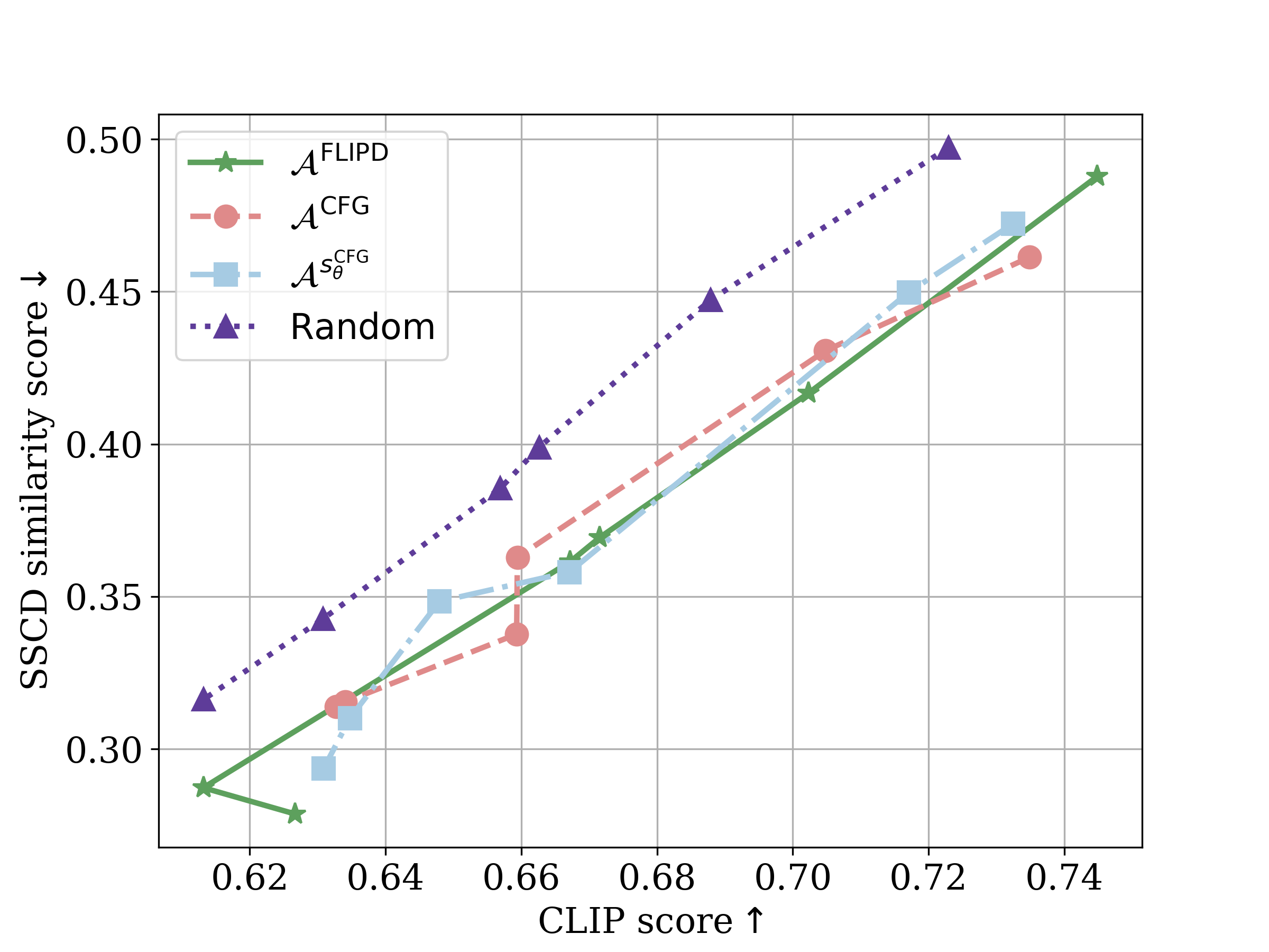
(a) Analysis of the mitigation approach.

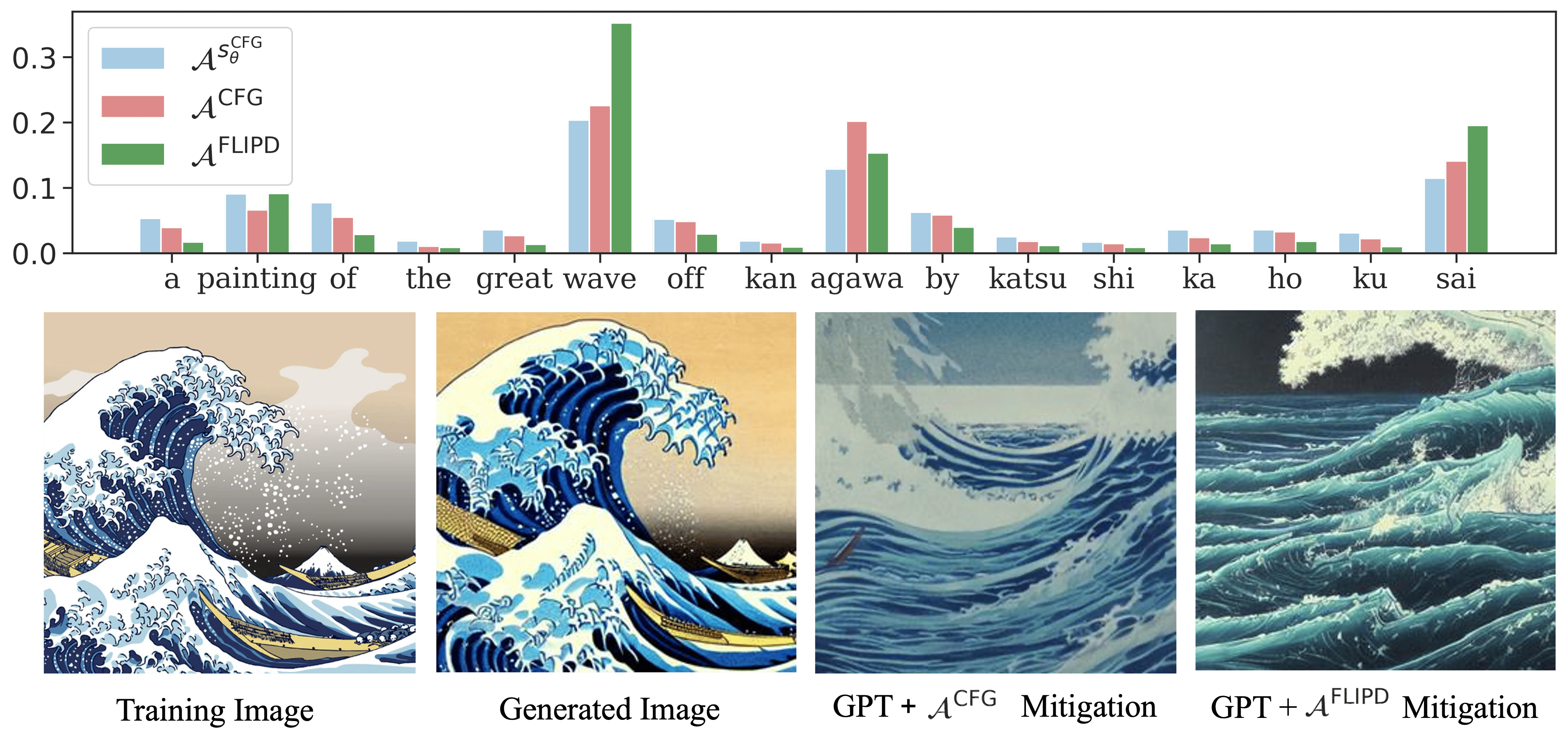
(b) Comparing (normalized) token attributions for a memorized prompt using three methods.

Figure 7: Using token attributions to detect drivers of memorization and to mitigate it at sample time.

5 Related Work

Detecting and Preventing Memorization for Image Models

The task of surfacing memorized samples is well-studied. Consensus in the literature is that $\ell_{2}$ distance to the nearest training sample in pixel space is a poor detector of memorized samples (Carlini et al., 2023), but that recalibrating the $\ell_{2}$ distance according to the local concentration of the dataset works better for smaller datasets (Yoon et al., 2023; Stein et al., 2023), and that using retrieval techniques such as distance in SSCD feature space (Pizzi et al., 2022) works better still, especially for more complex, higher-resolution images (Somepalli et al., 2023a). However, all of these retrieval techniques are too expensive to be used to withhold samples from a live model. To more efficiently prevent memorized samples from being generated, past and concurrent works have altered the sampling procedure, training procedure, or the model itself (Wen et al., 2023; Daras et al., 2024; Chen et al., 2024; Hintersdorf et al., 2024).

Explaining Memorization

There is an active community effort attempting to explain why and how memorization occurs in DGMs. Early studies focused on GANs, and have taken both theoretical (Nagarajan et al., 2018) and empirical (Bai et al., 2021) perspectives. However, GANs are thought to be less prone to memorization than DMs (Akbar et al., 2023), except on small datasets (Feng et al., 2021). Several works on DMs (Pidstrigach, 2022; Yi et al., 2023; Gu et al., 2023; Li et al., 2024) have pointed out that, given sufficient capacity, DMs at optimality are capable of learning the empirical training distribution, which is complete memorization. Others have focused on generalization, showing that DMs are capable of generalizing well in theory (Li et al., 2023), have inductive biases towards generating photorealistic images (Kadkhodaie et al., 2024), and will generalize when their capacity is insufficient to memorize (Yoon et al., 2023).

DGM-Based LID Estimation

As opposed to statistical LID estimators (e.g., Levina & Bickel (2004)), which are constructed to estimate the dimension of $\mathcal{M}_{*}$, DGM-based ones estimate the dimensionality of $\mathcal{M}_{\theta}$, the manifold learned by a DGM. These types of estimators are available for many types of DGMs, and in addition to being useful for memorization, have found utility in out-of-distribution detection (Kamkari et al., 2024a). In the literature, LID estimators for normalizing flows (Dinh et al., 2014) have been proposed using the singular values of their Jacobians (Horvat & Pfister, 2022; Kamkari et al., 2024a) or their density estimates (Tempczyk et al., 2022). In Section 4 we apply the singular value method to obtain LID estimates for GANs. Dai & Wipf (2019) and Zheng et al. (2022) proposed estimators for VAEs (Kingma & Welling, 2014; Rezende et al., 2014) using the structure of their posterior distribution. Several authors have proposed estimators for DMs as well (Stanczuk et al., 2024; Kamkari et al., 2024b; Horvat & Pfister, 2024); we focus on those of Stanczuk et al. (2024) and Kamkari et al. (2024b) because they work with off-the-shelf DMs and do not require modifying the training procedure.

6 Conclusions, Limitations, and Future Work

Throughout this work, we have drawn connections between the geometry of a DGM and its propensity to memorize through the MMH. First, we showed that the notion of LID provides a systematic way of understanding different types of memorization. Second, we explained how memorization phenomena described by prior work can be understood from the perspective of LID. Third, we verified the MMH empirically across scales of data and classes of models. Fourth, we showed that controlling $\text{LID}_{\theta}$ is a promising way to mitigate memorization. We offered several connections, including the insight that some instances of memorization in DMs are due to the DM’s inability to generalize (OD-Mem), whereas others are due to low-LID ground truth (DD-Mem).

Despite having demonstrated the utility of the MMH as a principled avenue to detect and alleviate memorization, our current approaches can be improved: estimates of $\text{LID}_{\theta}$ have some overlap between memorized and not memorized samples, and our sample-time scheme for mitigating memorization using $\mathcal{A}^{\text{FLIPD}}(c)$ performs on par, but does not outperform, its more ad-hoc baseline using $\mathcal{A}^{\text{CFG}}(c)$. We expect future work to find even better ways of leveraging the MMH and LID towards these goals, e.g. by improving LID estimation, or by more efficiently controlling LID during sampling. Finally, although the manifold hypothesis does not apply directly to discrete data such as language, some intuitions described in this work carry over, and generalizations or parallels to the concepts here may offer insights for the language-modelling space.

Reproducibility Statement

To ensure the reproducibility of our experiments, we provide two links to our codebases. The first codebase, accessible at github.com/layer6ai-labs/dgm_geometry, contains our small-scale synthetic experiments, as well as the CIFAR10 experiments. The second, accessible at github.com/layer6ai-labs/diffusion_memorization/, extends the work in Wen et al. (2023) by incorporating functionalities inspired by the MMH to detect and mitigate memorization. Comprehensive details of our experimental setup are provided across Section 4, Appendix C, and Appendix D. All datasets used in our experiments are freely available from the referenced sources and are utilized in compliance with their respective licenses.

Ethics Statement

We do not foresee any ethical concerns with the present research. The overarching topic, memorization in generative models, is widely studied to better understand safety concerns associated with using and deploying such models. Our goal is to theoretically explain and to empirically detect and alleviate this phenomenon; we do not promote the use of these models for harmful practices.

Acknowledgments

We thank Kin Kwan Leung for his valuable help in proving E.4.

Appendix A Contextualizing the MMH within Definitions of Memorization

An Overview of Definitions

The MMH describes the mechanism through which memorization occurs. How does this mechanism fit into prior definitions of memorization from the literature? Formal definitions of memorization generally follow the same template: a point $x_{0}$ is memorized when the model’s probability measure $P_{\theta}$ places too much mass within some distance of $x_{0}$. Some of these definitions define memorization globally on the level of an entire model (Meehan et al., 2020; Yoon et al., 2023; Gu et al., 2023), while others define memorization locally for individual datapoints (Carlini et al., 2023; Bhattacharjee et al., 2023). The identical definitions of Yoon et al. (2023) and Gu et al. (2023) consider a point to be memorized based purely on a distance threshold; in practice, however, distances alone have been unsuccessful at consistently surfacing what would be perceived by humans as memorized (Somepalli et al., 2023a; Stein et al., 2023). We postulate this is also due to manifold structure; semantically memorized images such as Figure 2 will sit on the same manifold, but may not necessarily be close to each other as measured by distance, even when taken in the latent space of an encoder. Meanwhile, Carlini et al. (2023) take a privacy perspective; their definition considers images memorized if they can be extracted from a model by any means, not just generated by the model. In this work we take the perspective that memorized samples are most likely to be problematic when they are generated by a production model, which are often treated as a black-box, so we focus on generation rather than extraction.

Links Between Formal Memorization and the MMH

For the reasons above, we use here the definition of memorization by Bhattacharjee et al. (2023), who define a point $x_{0}$ as memorized by comparing $P_{\theta}$ to the ground truth $P_{*}$ in a neighbourhood of $x_{0}$. We present their definition here:

Definition A.1.

Let $P_{*}$ and $P_{\theta}$ be the ground truth and model probability measures, respectively. Let $\lambda>1$ and $0<\gamma<1$. A point $x\in\mathbb{R}^{d}$ is a $(\lambda,\gamma)$-copy of a training datapoint $x_{0}$ if there exists a radius $r>0$ such that the $d$-dimensional ball $B_{r}^{d}(x_{0})$ of radius $r$ centred at $x_{0}$ satisfies $(i)\ x\in B_{r}^{d}(x_{0})$, $(ii)\ P_{\theta}(B_{r}^{d}(x_{0}))\geq\lambda P_{*}(B_{r}^{d}(x_{0}))$, and $(iii)\ P_{*}(B_{r}^{d}(x_{0}))\leq\gamma$.

The first and third conditions imply that $x$ is sufficiently close to $x_{0}$ relative to the amount of probability mass in the region ($P_{*}(B_{r}(x_{0}))$), while the second condition implies that the model $P_{\theta}$ places much more mass in the region compared to the ground truth $P_{*}$. A natural question about the MMH is whether points satisfying it are also formally memorized by the above definition. The answer is in the negative for DD-Mem (A.2) and the affirmative for OD-Mem (Theorem A.3).

Proposition A.2.

There exist models $p_{\theta}(x)$ that exhibit DD-Mem at $x_{0}\in\mathbb{R}^{d}$, but do not generate $(\lambda,\gamma)$-copies of $x_{0}$.

Proof.

Choose any ground truth distribution $P_{*}$ on a manifold $\mathcal{M}_{*}$ with a low-LID point $x_{0}\in\mathcal{M}_{*}$ (for example, set $\text{LID}_{*}(x_{0})=0$). A perfect model will exhibit DD-Mem at $x_{0}$, but for any ball $B_{r}^{d}(x_{0})$ containing $x_{0}$, $P_{\theta}(B_{r}^{d}(x_{0}))=P_{*}(B_{r}^{d}(x_{0}))$, violating the second condition of A.1. ∎

Since DD-Mem is a consequence of the data distribution having points $x_{0}$ with inherently low $\text{LID}_{*}(x_{0})$, these memorized points are likely to be generated even when there is no excess probability mass assigned near $x_{0}$ by $P_{\theta}$, as required in the definition of $(\lambda,\gamma)$-copies.

Theorem A.3 (Informal).

Suppose $x_{0}\in\mathbb{R}^{d}$ is such that $p_{\theta}(x)$ exhibits OD-Mem at $x_{0}$. Then, for every $\lambda>1$ and $0<\gamma<1$, $p_{\theta}(x)$ will generate $(\lambda,\gamma)$-copies of $x_{0}$ with near-certainty.

Proof.

See Appendix E for the formal statement of the theorem and proof. ∎

The MMH thus provides two important pieces of context for the definition of $(\lambda,\gamma)$-copies. The first is that A.1 is in some sense incomplete; it does not cover DD-Mem. The second is that OD-Mem can be considered a useful refinement of A.1. While the algorithm given by Bhattacharjee et al. (2023) is intractable at scale, we show in Section 4 that the added strength (in the mathematical sense) of the MMH allows us to flag memorized data more efficiently using only estimators of LID.

Appendix B LID Estimation

B.1 LID Estimation with Diffusion Models

As mentioned in the main manuscript, we follow the SDE framework of Song et al. (2021) for DMs, where the so called forward SDE is given by

$${\textnormal{d}}x_{t}=f(x_{t},t){\textnormal{d}}t+g(t){\textnormal{d}}W_{t},\quad x_{0}\sim p_{*}(x),$$ (3)

where $f:\mathbb{R}^{d}\times[0,1]\rightarrow\mathbb{R}^{d}$ and $g:[0,1]\rightarrow\mathbb{R}$ are pre-specified functions and $W_{t}$ is a Brownian motion on $\mathbb{R}^{d}$. This process progressively adds noise to data from $p_{*}(x)$, and we denote the distribution of $x_{t}$ as $p_{t}(x_{t})$. This process can be reversed in time in the sense that if $y_{t}\coloneqq x_{1-t}$, then $y_{t}$ obeys the so called backward SDE,

$${\textnormal{d}}y_{t}=\left[g^{2}(1-t)\nabla\log p_{1-t}(y_{t})-f(y_{t},1-t)\right]{\textnormal{d}}t+g(1-t){\textnormal{d}}\tilde{W}_{t},\quad y_{0}\sim p_{1},$$ (4)

where $\tilde{W}_{t}$ is another Brownian motion. DMs aim to learn the (Stein) score function, $\nabla\log p_{t}(x_{t})$, by approximating it with a neural network $s_{\theta}:\mathbb{R}^{d}\times(0,1]\rightarrow\mathbb{R}^{d}$. Once the network is trained, $s_{\theta}(x_{t},t)\approx\nabla\log p_{t}(x_{t})$ is plugged in Equation 4, and solving the resulting SDE allows to transform noise into model samples. Below we briefly summarize two existing methods, FLIPD and NB, for approximating $\text{LID}_{\theta}(x)$ for a DM.

FLIPD Kamkari et al. (2024b) proposed FLIPD, an estimator of $\text{LID}_{\theta}(x)$ for DMs. Commonly $f$ is linear in $x_{t}$, in which case the transition kernel corresponding to the forward SDE is given by

$$p_{t\mid 0}(x_{t}\mid x_{0})=\mathcal{N}(x_{t};\psi(t)x_{0},\sigma^{2}(t)I_{d}),$$ (5)

where $\psi,\sigma:[0,1]\rightarrow\mathbb{R}$ are known functions which depend on the choices of $f$ and $g$, and which can be easily evaluated. For a DM with such a transition kernel, FLIPD is defined as

$$\text{FLIPD}(x,t_{0})=d+\sigma^{2}(t_{0})\Big{(}\text{tr}\left(\nabla s_{\theta}\big{(}\psi(t_{0})x,t_{0}\big{)}\right)+\lVert s_{\theta}\big{(}\psi(t_{0})x,t_{0}\big{)}\rVert^{2}\Big{)},$$ (6)

where $t_{0}\in[0,1]$ is a hyperparameter. Kamkari et al. (2024b) proved that, when $t_{0}\approx 0$ and $x\in\mathcal{M}_{\theta}$, $\text{FLIPD}(x,t_{0})$ is a valid approximation of $\text{LID}_{\theta}(x)$. The reason for this is that the rate of change of the log density of the convolution between $p_{\theta}(x)$ and a Gaussian evaluated at $x_{0}$ with respect to the amount of added Gaussian noise approximates $\text{LID}_{\theta}(x_{0})$; and Kamkari et al. (2024b) showed that FLIPD computes this rate of change. In practice computing the trace of the Jacobian of $s_{\theta}$ is the only expensive operation needed to compute FLIPD, and this is easily approximated by using the Hutchinson stochastic trace estimator (Hutchinson, 1989).

NB  Stanczuk et al. (2024) proposed another estimator of $\text{LID}_{\theta}(x)$ for DMs. Following Kamkari et al. (2024b), we refer to this estimator as the normal bundle (NB) estimator. Stanczuk et al. (2024) proved that when $f(x_{t},t)\equiv 0$, $s_{\theta}(x_{t},t)$ points orthogonally towards $\mathcal{M}_{\theta}$ as $t\rightarrow 0$. They leverage this observation as follows: for a given $x$, Equation 3 is started at $x$ and run forward until time $t_{0}$; this is done $k$ times, resulting in $x_{t_{0}}^{(1)},\dots,x_{t_{0}}^{(k)}$. The matrix $S_{\theta}(x,t_{0})\in\mathbb{R}^{d\times k}$ is then constructed as

$$S_{\theta}(x,t_{0})=\left[s_{\theta}\left(x_{t_{0}}^{(1)},t_{0}\right)\middle|\cdots\middle|s_{\theta}\left(x_{t_{0}}^{(k)},t_{0}\right)\right],$$ (7)

and thanks to the previous observation, the columns of $S_{\theta}(x,t_{0})$ approximately span the normal space of $\mathcal{M}_{\theta}$ at $x$ when $t_{0}\approx 0$, meaning that $\text{rank }S_{\theta}(x,t_{0})\approx d-\text{LID}_{\theta}(x)$. The NB estimator is given by

$$\text{NB}(x,t_{0})=d-\text{rank }S_{\theta}(x,t_{0}).$$ (8)

In practice the rank is numerically computed by setting a threshold, carrying out a singular value decomposition of $S_{\theta}(x,t_{0})$, and counting the number of singular values above the threshold. Stanczuk et al. (2024) recommend setting $k=4d$, and we follow this recommendation. Computing the NB estimator is much more expensive than FLIPD, since $4d$ forward calls have to be made to construct $S_{\theta}(x,t_{0})$, and then the singular value decomposition has a cost which is cubic in $d$. Finally, we point out that when $f$ is not identically equal to $0$, the NB method can be easily adapted to still provide a valid approximation of $\text{LID}_{\theta}(x)$ (Kamkari et al., 2024a).

We highlight that both FLIPD and NB were originally developed as estimators of $\text{LID}_{*}(x)$ under the view that if the learned score function is a good approximation of the true score function, then $\text{LID}_{\theta}(x)\approx\text{LID}_{*}(x)$. In our work, we see these methods as approximating $\text{LID}_{\theta}(x)$. Note that these views are not contradictory: when the DM properly approximates the true score function, it will indeed be the case that $\text{LID}_{\theta}(x)\approx\text{LID}_{*}(x)$; importantly though, when this approximation fails, we interpret $\text{FLIPD}(x,t_{0})$ and $\text{NB}(x,t_{0})$ as still providing a valid approximation of $\text{LID}_{\theta}(x)$ rather than a poor estimate of $\text{LID}_{*}(x)$.

B.2 Local Principal Component Analysis

Local PCA (Fukunaga & Olsen, 1971) offers a straightforward method for estimating the $\text{LID}_{*}$ of a datapoint by using linear local approximations to the data manifold. Given $x$, local PCA first identifies a set of nearby points in the dataset, representing a neighbourhood; this is typically done through a $k$-nearest neighbours algorithm. Next, the algorithm performs a principal component analysis (PCA) on this neighbourhood to get $(i)$ principal components and $(ii)$ explained variances for each component; the resulting principal components capture the directions of data variation, with the explained variance showing the amount of variation along each direction. Directions off the manifold are expected to have negligible explained variance. Hence, local PCA determines the number of components with non-zero (or non-negligible) explained variance as an estimate for $\text{LID}_{*}(x)$.

B.3 LID Estimation with GANs

We assume the GAN is given by a generator $G_{\theta}:\mathbb{R}^{d^{\prime}}\to\mathbb{R}^{d}$ which transforms latent variables from a distribution in $\mathbb{R}^{d^{\prime}}$ to the ambient space $\mathbb{R}^{d}$. For a generated sample $x=G_{\theta}(z)$, we estimate $\text{LID}_{\theta}(x)$ as the rank of the Jacobian of the generator, i.e. $\text{rank }\nabla G_{\theta}(z)$. As for the NB estimator with DMs, the rank is numerically computed by thresholding singular values. We highlight that this is a standard approach to estimate $\text{LID}_{\theta}$ in decoder-based DGMs (Horvat & Pfister, 2022; Kamkari et al., 2024a; Humayun et al., 2024).

Appendix C Experimental Details

C.1 Hyper-parameter Setup for LID Estimation Methods

$\widehat{\text{LID}}_{*}$ with Local PCA

As established in Appendix B.2, local PCA estimates the intrinsic dimensionality of a datapoint by counting the number of significant explained variances from a PCA performed on the datapoint’s local neighbourhood, determined by its $k$ nearest neighbours ($k=100$ in our experiments). Finding the significant explained variances is done through a threshold hyperparameter, $\tau$, where explained variances above $\tau$ are considered significant. For our approach in 5(d), we introduce two key modifications to better adapt the original Local PCA algorithm for detecting DD-Mem: $(i)$ instead of selecting $\tau$ individually for each datapoint, we define it globally as the $10$th percentile of all explained variances across the entire dataset; $(ii)$ if a datapoint has neighbours within the $10$th percentile of all pairwise distances, we restrict the neighbourhood to those points. The second modification allows us to avoid including distant points in the neighbourhood if closer ones already exist and especially helps us detect zero-dimensional point masses.

$\widehat{\text{LID}}_{\theta}$ for GANs

As detailed in Appendix B.3, the rank of the Jacobian $\nabla G_{\theta}(z)$ can be used to estimate $\widehat{\text{LID}}_{\theta}$. However, in practice, the rank — or, equivalently, the number of non-zero singular values — tends to equal the latent dimension; this is because singular values are typically close to zero but rarely exactly zero. To account for this, we apply a thresholding approach: a singular value is considered significant (non-zero) if it exceeds a hyperparameter $\tau$. We define $\tau$ as the 10th percentile of all singular values computed from the generated images in 5(b) and 8(b).

$\widehat{\text{LID}}_{\theta}$ with NB

We used $t_{0}=0.1$ and thresholded the singular values of $S_{\theta}(x,t_{0})$ by 10th percentile; the results are presented in 5(c) and 8(a). The choice of $t_{0}$ is empirically determined by observing how the NB score correlates with the memorization behavior with a fixed subset of 1000 randomly generated samples.

$\widehat{\text{LID}}_{\theta}$ with FLIPD

Unless stated otherwise, we set $t_{0}=0.05$ for FLIPD and use the Hutchinson trace estimator to approximate the trace of the score gradient in Equation 6. In line with Kamkari et al. (2024b), we apply this in the latent space of Stable diffusion and use a single Hutchinson sample to estimate Equation 6 for all of our large-scale experiments.

CFG Norm for Detecting Memorized Samples in the Training Set

Note that while Wen et al. (2023) use the generation process to measure whether a synthesized image has been memorized, we were interested in detecting whether real, training-set images have been memorized in Figure 6, which requires some methodological changes. To compute a memorization score, we take $k$ Euler steps forward using the conditional score $s_{\theta}(x;t,c)$ with the probability flow ODE (Song et al., 2021) until time $t_{0}$ to get a point at $x_{0}\in\mathbb{R}^{d}$. We then compute the CFG norm $\lVert s_{\theta}(x_{0};t_{0},c)-s_{\theta}(x;t_{0},\emptyset)\rVert$. We use timestep $t_{0}=0.01$ and 3 Euler steps.

C.2 The Confounding Effect of Complexity for Detecting Memorization

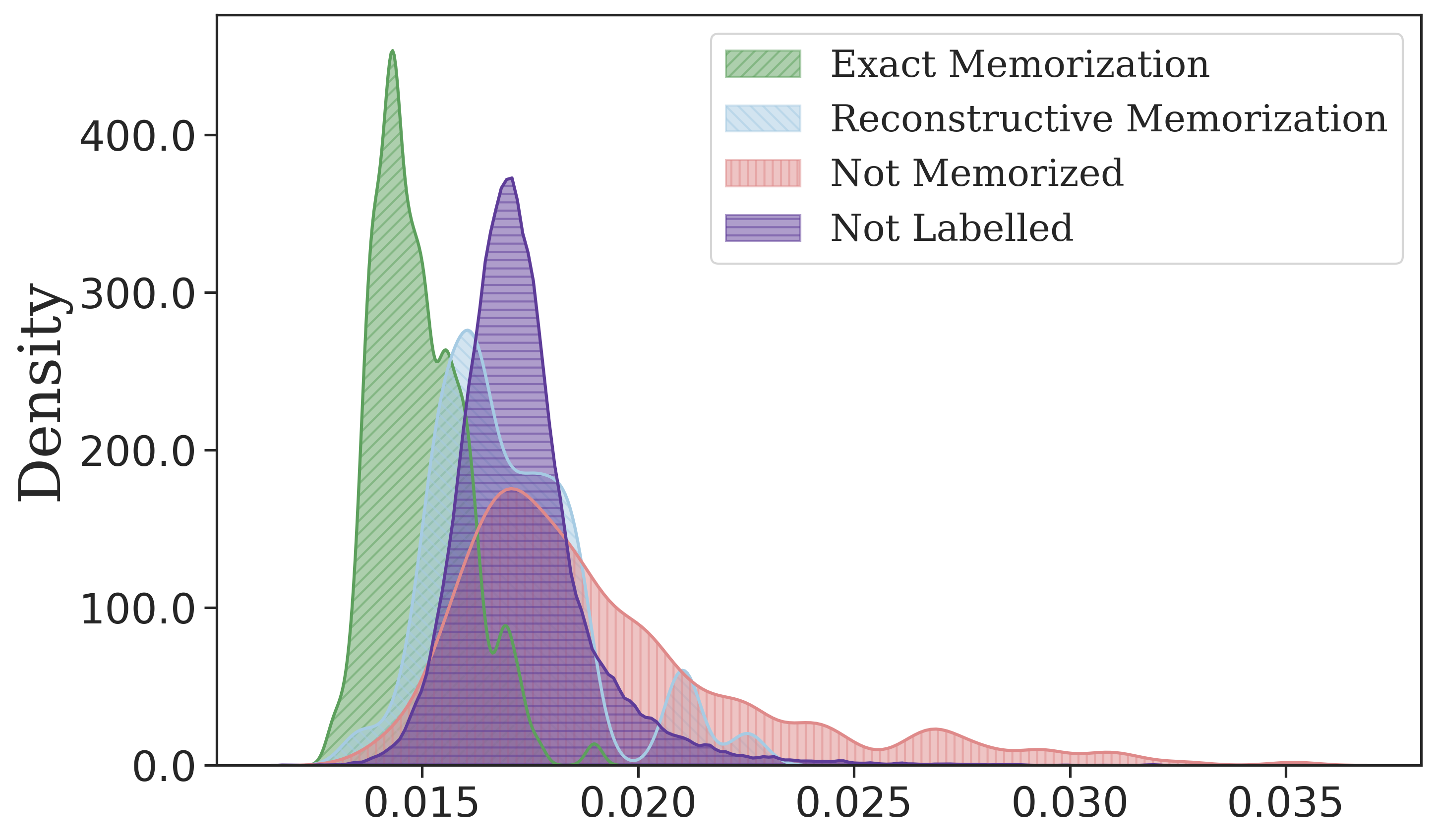
(a) $\widehat{\text{LID}}_{\theta}$ adjusted by PNG for iDDPM.
 

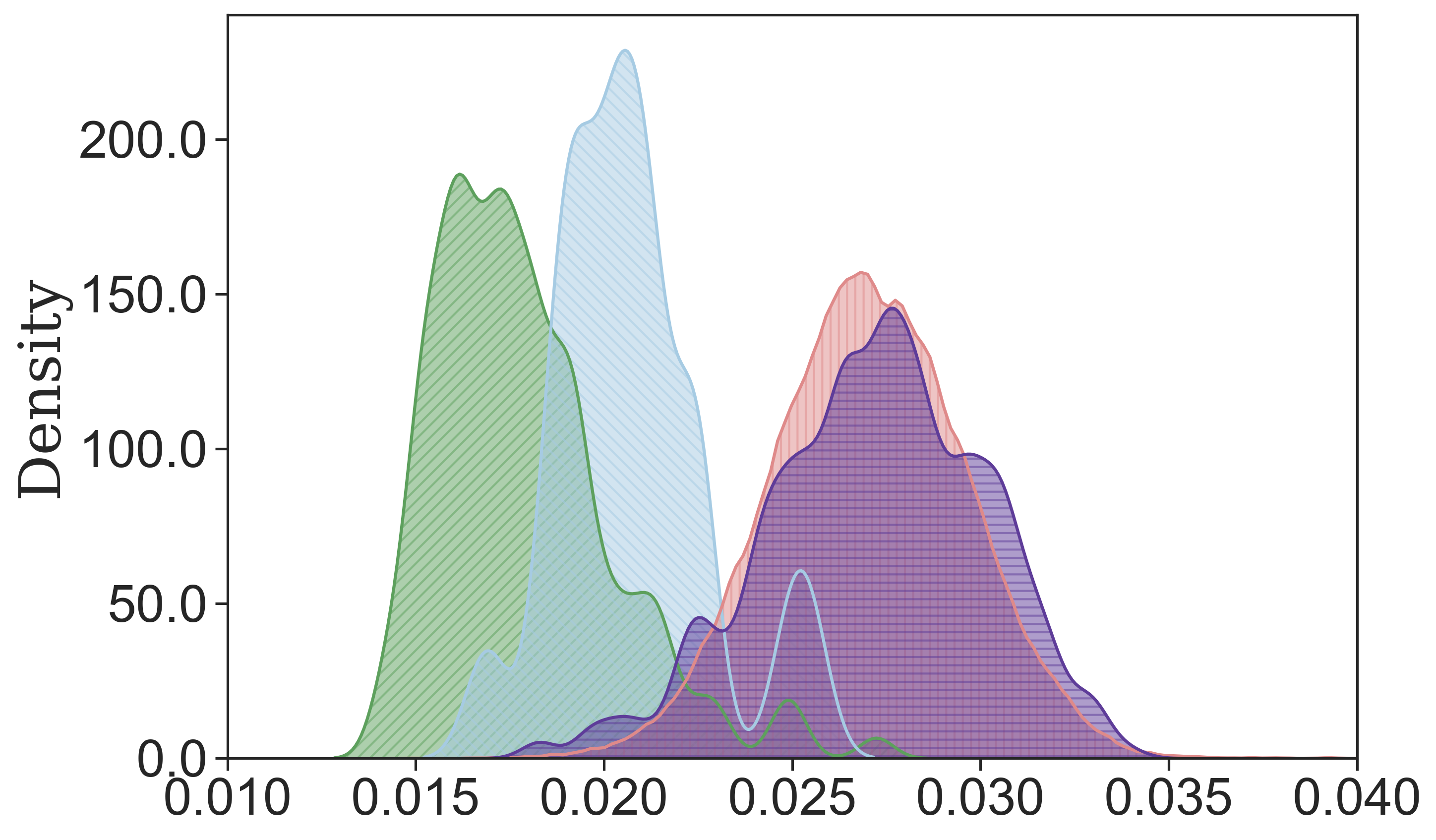
(b) $\widehat{\text{LID}}_{\theta}$ adjusted by PNG for StyleGAN-ADA2.
 

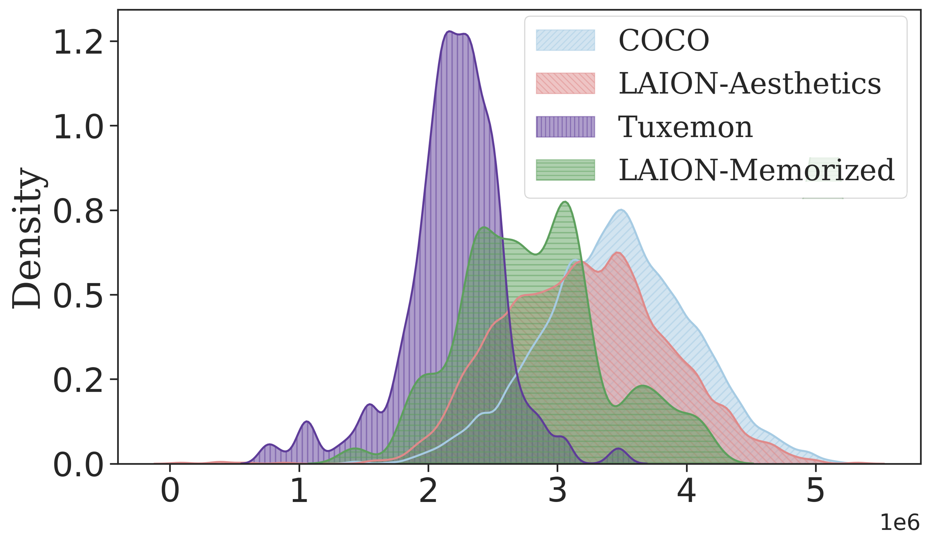
(c) PNG compression length for Stable Diffusion images.

Figure 8: Removing and analyzing image complexity as a confounding factor in memorization detection for CIFAR10 (a-b) and Stable Diffusion (c).

$\text{LID}_{\theta}$ is correlated with image complexity (Section 2; Kamkari et al. (2024b)), which raises a valid concern: the correlation, combined with the fact that simpler images are more likely to be memorized, suggests that image complexity may confound our analysis. This is evident in 5(a) (right panel), where GAN-generated images with the lowest $\widehat{\text{LID}}_{\theta}$ values are the simplest ones, not necessarily the memorized ones. To address this confounding factor, we draw inspiration from Kamkari et al. (2024b) and normalize it by PNG compression length, using it as a proxy for image complexity. We use the maximum compression level of 9 with the cv2 package (Bradski, 2000). According to this adjusted metric, the smallest values now correspond to memorized images that are not necessarily simple, such as the cars in CIFAR10. 8(a) and 8(b) show these adjusted LID estimated values, which achieve a slightly improved separation between memorized and not memorized images (as well as between exactly memorized and reconstructively memorized images) than the non-PNG-normalized results in the main text. It is worth noting that complexity did not appear to be a confounding factor in the Stable Diffusion analysis shown in Figure 6. In fact, as depicted in 8(c), the Tuxemon images are relatively simpler than the LAION memorized images, as measured by their PNG compression length. However, despite their simplicity, Tuxemon images have consistently higher $\widehat{\text{LID}}_{\theta}$ values compared to the memorized images in 6(b) and 6(a).

Appendix D Text Conditioning and Memorization in Stable Diffusion

D.1 Adapting Denoising Diffusion Probabilistic and Implicit Models

Following Wen et al. (2023), we use denoising diffusion probabilistic models (DDPMs) (Ho et al., 2020). This model can be seen as a discretization of the forward SDE process of a score-based DM (Song et al., 2021). Here, instead of continuous timesteps $t$, a timestep ${\color[rgb]{0.8745098039215686,0.5411764705882353,0.5411764705882353}t}$ instead belongs to a sequence $\{0,\ldots{\color[rgb]{0.8745098039215686,0.5411764705882353,0.5411764705882353}T}\}$ with ${\color[rgb]{0.8745098039215686,0.5411764705882353,0.5411764705882353}T}$ being the largest timescale; we use ${\color[rgb]{0.8745098039215686,0.5411764705882353,0.5411764705882353}T}=50$. We use the colour red to denote the discretized notation used in Ho et al. (2020).

With that in mind, DDPMs can be seen as a Markov noising process with the following transition kernel, parameterized by ${\color[rgb]{0.8745098039215686,0.5411764705882353,0.5411764705882353}\bar{\alpha}_{t}}$, mirroring the notation from Ho et al. (2020):

$${\color[rgb]{0.8745098039215686,0.5411764705882353,0.5411764705882353}p_{t\mid 0}}({\color[rgb]{0.8745098039215686,0.5411764705882353,0.5411764705882353}x_{t}}\mid{\color[rgb]{0.8745098039215686,0.5411764705882353,0.5411764705882353}x_{0}})\coloneqq\mathcal{N}(x_{t};\sqrt{{\color[rgb]{0.8745098039215686,0.5411764705882353,0.5411764705882353}\bar{\alpha}_{t}}}\cdot{\color[rgb]{0.8745098039215686,0.5411764705882353,0.5411764705882353}x_{0}},(1-{\color[rgb]{0.8745098039215686,0.5411764705882353,0.5411764705882353}\bar{\alpha}_{t}})\mathbf{I}_{d}).$$ (9)

DDPMs do not directly parameterize the score function, but rather use a neural network ${\color[rgb]{0.8745098039215686,0.5411764705882353,0.5411764705882353}\epsilon_{\theta}}({\color[rgb]{0.8745098039215686,0.5411764705882353,0.5411764705882353}x_{t}},{\color[rgb]{0.8745098039215686,0.5411764705882353,0.5411764705882353}t})$, which relates to the score function as:

$$s_{\theta}(x,{\color[rgb]{0.8745098039215686,0.5411764705882353,0.5411764705882353}t}/{\color[rgb]{0.8745098039215686,0.5411764705882353,0.5411764705882353}T})=-{\color[rgb]{0.8745098039215686,0.5411764705882353,0.5411764705882353}\epsilon_{\theta}}(x,{\color[rgb]{0.8745098039215686,0.5411764705882353,0.5411764705882353}t})/\sqrt{1-{\color[rgb]{0.8745098039215686,0.5411764705882353,0.5411764705882353}\bar{\alpha}_{t}}}\text{, or equivalently, }-\sigma({\color[rgb]{0.8745098039215686,0.5411764705882353,0.5411764705882353}t}/{\color[rgb]{0.8745098039215686,0.5411764705882353,0.5411764705882353}T})s_{\theta}(x,{\color[rgb]{0.8745098039215686,0.5411764705882353,0.5411764705882353}t}/{\color[rgb]{0.8745098039215686,0.5411764705882353,0.5411764705882353}T})={\color[rgb]{0.8745098039215686,0.5411764705882353,0.5411764705882353}\epsilon_{\theta}}(x,{\color[rgb]{0.8745098039215686,0.5411764705882353,0.5411764705882353}t}).$$ (10)

Note that in this context, we have $\sigma^{2}({\color[rgb]{0.8745098039215686,0.5411764705882353,0.5411764705882353}t}/{\color[rgb]{0.8745098039215686,0.5411764705882353,0.5411764705882353}T})=1-{\color[rgb]{0.8745098039215686,0.5411764705882353,0.5411764705882353}\bar{\alpha}_{t}}$ and $\psi({\color[rgb]{0.8745098039215686,0.5411764705882353,0.5411764705882353}t}/{\color[rgb]{0.8745098039215686,0.5411764705882353,0.5411764705882353}T})=\sqrt{{\color[rgb]{0.8745098039215686,0.5411764705882353,0.5411764705882353}\bar{\alpha}_{t}}}$. Equation 9 (the transition kernel) and Equation 10 (the score function) provide us with the recipe for estimating $\text{LID}_{\theta}$ using FLIPD with DDPMs (recall Equation 6).

When sampling from DMs we use the DDIM sampler (Song et al., 2020), mirroring the setup in Wen et al. (2023). In our notation, this sampler defines $\tilde{x}_{t}\coloneqq x_{t}/\psi(t)$, where $x_{t}$ is given as in Equation 3. In turn, $\tilde{x}_{t}$ obeys the forward SDE:

$${\textnormal{d}}\tilde{x}_{t}=\tilde{g}(t){\textnormal{d}}W_{t},\quad\tilde{x}_{0}\sim p_{*}(x),$$ (11)

where $\tilde{g}(t)=g(t)/\psi(t)$. This SDE has a corresponding score function

$$\tilde{s}_{\theta}(x,t)=\psi(t)s_{\theta}\big{(}\psi(t)x,t\big{)},$$ (12)

and DDIM uses this score function to sample from the model. The transition kernel corresponding to Equation 11 has $\tilde{\psi}(t)=1$ and a $\tilde{\sigma}(t)$ which can be computed in closed form. Analogously to Equation 10, we can define ${\color[rgb]{0.8745098039215686,0.5411764705882353,0.5411764705882353}\tilde{\epsilon}_{\theta}}$ as

$${\color[rgb]{0.8745098039215686,0.5411764705882353,0.5411764705882353}\tilde{\epsilon}_{\theta}}(x,{\color[rgb]{0.8745098039215686,0.5411764705882353,0.5411764705882353}t})=-\tilde{\sigma}({\color[rgb]{0.8745098039215686,0.5411764705882353,0.5411764705882353}t}/{\color[rgb]{0.8745098039215686,0.5411764705882353,0.5411764705882353}T})\tilde{s}_{\theta}(x,{\color[rgb]{0.8745098039215686,0.5411764705882353,0.5411764705882353}t}/{\color[rgb]{0.8745098039215686,0.5411764705882353,0.5411764705882353}T}).$$ (13)

We highlight that FLIPD (Equation 6) can be applied using the forward SDE in Equation 11 along with its corresponding score function in Equation 12, resulting in the estimate

$$\widetilde{\text{FLIPD}}(x,t)=d+\tilde{\sigma}^{2}(t)\Big{(}\text{tr}\left(\nabla\tilde{s}_{\theta}\big{(}x,t\big{)}\right)+\lVert\tilde{s}_{\theta}\big{(}x,t\big{)}\rVert^{2}\Big{)}.$$ (14)

Note that this estimate can be computed when having access to ${\color[rgb]{0.8745098039215686,0.5411764705882353,0.5411764705882353}\tilde{\epsilon}_{\theta}}$ thanks to Equation 13. We also note that in our text-conditioning analysis, we are interested in the probabilities conditioned by the text prompt, thus, these score functions are extended by the conditioning variable $c$, resulting in the modified forms ${\color[rgb]{0.8745098039215686,0.5411764705882353,0.5411764705882353}\epsilon_{\theta}}(x;{\color[rgb]{0.8745098039215686,0.5411764705882353,0.5411764705882353}t},c)$, ${\color[rgb]{0.8745098039215686,0.5411764705882353,0.5411764705882353}\tilde{\epsilon}_{\theta}}(x;{\color[rgb]{0.8745098039215686,0.5411764705882353,0.5411764705882353}t},c)$, $s_{\theta}(x;{\color[rgb]{0.8745098039215686,0.5411764705882353,0.5411764705882353}t}/{\color[rgb]{0.8745098039215686,0.5411764705882353,0.5411764705882353}T},c)$, and $\tilde{s}_{\theta}(x;{\color[rgb]{0.8745098039215686,0.5411764705882353,0.5411764705882353}t}/{\color[rgb]{0.8745098039215686,0.5411764705882353,0.5411764705882353}T},c)$.

D.2 Unifying Differentiable Metrics for Text-conditioned Memorization

We begin by revisiting the differentiable memorization metric used by Wen et al. (2023) for detecting and mitigating memorization, reformulating it within the continuous, score-based framework of diffusion models. Building on this, we perform an analysis, making minimal modifications to the original formulation to derive alternative metrics that remain effective and are theoretically-grounded. As a result, here we will formally derive three differentiable metrics: $\mathcal{A}^{\text{CFG}}(c)$, $\mathcal{A}^{s_{\theta}^{\text{CFG}}}(c)$, and finally $\mathcal{A}^{\text{FLIPD}}(c)$. We show that the value Wen et al. (2023) compute in their paper is in fact an estimator of $\mathcal{A}^{\text{CFG}}(c)$, rescaled by a constant. We then make minor modifications to introduce the two new metrics $\mathcal{A}^{s_{\theta}^{\text{CFG}}}(c)$ and $\mathcal{A}^{\text{FLIPD}}$ and interpret them through the lens of the MMH. Finally, our results show that all these metrics perform on par with the original one by Wen et al. (2023).

The Differentiable Metric by Wen et al. (2023)

For any text condition $c$, Wen et al. (2023) generate multiple samples $({\color[rgb]{0.8745098039215686,0.5411764705882353,0.5411764705882353}\tilde{x}_{0}}^{(n)})_{n=1}^{N}$, with the $n$th sample following the (DDIM) trajectory $\{{\color[rgb]{0.8745098039215686,0.5411764705882353,0.5411764705882353}\tilde{x}_{T}}^{(n)},{\color[rgb]{0.8745098039215686,0.5411764705882353,0.5411764705882353}\tilde{x}_{T-1}}^{(n)},\ldots,{\color[rgb]{0.8745098039215686,0.5411764705882353,0.5411764705882353}\tilde{x}_{0}}^{(n)}\}$ from noise to data through the denoising process. They then introduce the following metric, which we have slightly reformulated to match our notation:

$${\color[rgb]{0.8745098039215686,0.5411764705882353,0.5411764705882353}\mathcal{A}^{\text{CFG}}}(c;N,{\color[rgb]{0.8745098039215686,0.5411764705882353,0.5411764705882353}T}) =\frac{1}{{\color[rgb]{0.8745098039215686,0.5411764705882353,0.5411764705882353}T}N}\sum_{n=1}^{N}\sum_{{\color[rgb]{0.8745098039215686,0.5411764705882353,0.5411764705882353}t}=0}^{{\color[rgb]{0.8745098039215686,0.5411764705882353,0.5411764705882353}T}}\lVert{\color[rgb]{0.8745098039215686,0.5411764705882353,0.5411764705882353}\tilde{\epsilon}_{\theta}}\left({\color[rgb]{0.8745098039215686,0.5411764705882353,0.5411764705882353}\tilde{x}_{t}}^{(n)};{\color[rgb]{0.8745098039215686,0.5411764705882353,0.5411764705882353}t},c\right)-{\color[rgb]{0.8745098039215686,0.5411764705882353,0.5411764705882353}\tilde{\epsilon}_{\theta}}\left({\color[rgb]{0.8745098039215686,0.5411764705882353,0.5411764705882353}\tilde{x}_{t}}^{(n)};{\color[rgb]{0.8745098039215686,0.5411764705882353,0.5411764705882353}t},\emptyset\right)\rVert^{2}.$$ (15)

We colour-code the metric in red to distinguish between it and the analogous metric that we will shortly derive at the end of this section.

Let $\tilde{p}_{t}^{\text{CFG}}(\cdot\mid c)$ represent the marginal probability at time $t$ induced by the DDIM sampler conditioned on $c$ with the addition of the CFG term. Recall that $\lambda$ denotes the “guidance strength”, and using Equation 13 and Equation 2, we can rewrite ${\color[rgb]{0.8745098039215686,0.5411764705882353,0.5411764705882353}\mathcal{A}^{\text{CFG}}}(c;N,{\color[rgb]{0.8745098039215686,0.5411764705882353,0.5411764705882353}T})$ as follows:

$${\color[rgb]{0.8745098039215686,0.5411764705882353,0.5411764705882353}\mathcal{A}^{\text{CFG}}}(c;N,{\color[rgb]{0.8745098039215686,0.5411764705882353,0.5411764705882353}T})\coloneqq\frac{1}{{\color[rgb]{0.8745098039215686,0.5411764705882353,0.5411764705882353}T}N}\sum_{n=1}^{N}\sum_{t=0}^{{\color[rgb]{0.8745098039215686,0.5411764705882353,0.5411764705882353}T}}\Big{\|}-\frac{\tilde{\sigma}({\color[rgb]{0.8745098039215686,0.5411764705882353,0.5411764705882353}t}/{\color[rgb]{0.8745098039215686,0.5411764705882353,0.5411764705882353}T})}{\lambda}\left[\tilde{s}_{\theta}^{\text{CFG}}({\color[rgb]{0.8745098039215686,0.5411764705882353,0.5411764705882353}\tilde{x}_{t}}^{(n)};{\color[rgb]{0.8745098039215686,0.5411764705882353,0.5411764705882353}t}/{\color[rgb]{0.8745098039215686,0.5411764705882353,0.5411764705882353}T},c)-\tilde{s}_{\theta}({\color[rgb]{0.8745098039215686,0.5411764705882353,0.5411764705882353}\tilde{x}_{t}}^{(n)};{\color[rgb]{0.8745098039215686,0.5411764705882353,0.5411764705882353}t}/{\color[rgb]{0.8745098039215686,0.5411764705882353,0.5411764705882353}T},\emptyset)\right]\Big{\|}^{2}.$$ (16)

We now assume ${\color[rgb]{0.8745098039215686,0.5411764705882353,0.5411764705882353}T}\to\infty$, which will reformulate Equation 16 with an integral that we will replace with an expectation:

$${\color[rgb]{0.8745098039215686,0.5411764705882353,0.5411764705882353}\mathcal{A}^{\text{CFG}}}(c;N) \coloneqq\lim_{{\color[rgb]{0.8745098039215686,0.5411764705882353,0.5411764705882353}T}\to\infty}{\color[rgb]{0.8745098039215686,0.5411764705882353,0.5411764705882353}\mathcal{A}^{\text{CFG}}}(c;N,{\color[rgb]{0.8745098039215686,0.5411764705882353,0.5411764705882353}T})$$ (17)

$$=\lambda^{-2}\cdot\frac{1}{N}\sum_{n=1}^{N}\int_{0}^{1}\tilde{\sigma}^{2}(t)\lVert\tilde{s}_{\theta}^{\text{CFG}}({\color[rgb]{0.8745098039215686,0.5411764705882353,0.5411764705882353}\tilde{x}_{t}}^{(n)};t,c)-\tilde{s}_{\theta}({\color[rgb]{0.8745098039215686,0.5411764705882353,0.5411764705882353}\tilde{x}_{t}}^{(n)};t,\emptyset)\rVert^{2}\text{d}t$$ (18)

$$=\lambda^{-2}\cdot\frac{1}{N}\sum_{n=1}^{N}\mathbb{E}_{t\sim\mathcal{U}(0,1)}\left[\tilde{\sigma}^{2}(t)\lVert\tilde{s}_{\theta}^{\text{CFG}}({\color[rgb]{0.8745098039215686,0.5411764705882353,0.5411764705882353}\tilde{x}_{t}}^{(n)};t,c)-\tilde{s}_{\theta}({\color[rgb]{0.8745098039215686,0.5411764705882353,0.5411764705882353}\tilde{x}_{t}}^{(n)};t,\emptyset)\rVert^{2}\right]$$ (19)

$$=\lambda^{-2}\cdot\mathbb{E}_{t\sim\mathcal{U}(0,1)}\left[\frac{1}{N}\sum_{n=1}^{N}\tilde{\sigma}^{2}(t)\cdot\lVert\tilde{s}_{\theta}^{\text{CFG}}({\color[rgb]{0.8745098039215686,0.5411764705882353,0.5411764705882353}\tilde{x}_{t}}^{(n)};t,c)-\tilde{s}_{\theta}({\color[rgb]{0.8745098039215686,0.5411764705882353,0.5411764705882353}\tilde{x}_{t}}^{(n)};t,\emptyset)\rVert^{2}\right].$$ (20)

Here, $\mathcal{U}(0,1)$ denotes the uniform distribution. Next, we observe that the inner term of the expectation on the right-hand-side of Equation 20 is in fact a Monte-Carlo estimator. By the law of large numbers, we have the following:

$${\color[rgb]{0.8745098039215686,0.5411764705882353,0.5411764705882353}\mathcal{A}^{\text{CFG}}}(c) \coloneqq\lim_{N\to\infty}{\color[rgb]{0.8745098039215686,0.5411764705882353,0.5411764705882353}\mathcal{A}^{\text{CFG}}}(c;N)$$ (21)

$$=\lambda^{-2}\cdot\mathbb{E}_{t\sim\mathcal{U}(0,1)}\mathbb{E}_{\tilde{x}_{t}\sim\tilde{p}^{\text{CFG}}_{t}(\cdot\mid c)}\left[\tilde{\sigma}^{2}(t)\cdot\lVert\tilde{s}_{\theta}^{\text{CFG}}(\tilde{x}_{t};t,c)-\tilde{s}_{\theta}(\tilde{x}_{t};t,\emptyset)\rVert^{2}\right].$$ (22)

We now see that with the new formulation, all the red terms in Equation 22, have gone away, making it fully amenable to the score-based formulation of diffusion models. The $\lambda$ factor merely scales the metric, and for the purposes of detection and mitigation, this scaling is inconsequential: if a metric effectively predicts memorization, rescaling it will not diminish its effectiveness as a predictor. We thus disregard the scaling factor $\lambda$ to make the derivation cleaner and replace the uniform distribution $\mathcal{U}(0,1)$ with a general “scheduling” distribution $\mathcal{T}(0,1)$ of timesteps in $(0,1]$; this would allow our metric to be a generalization of the one proposed by Wen et al. (2023):

$$\mathcal{A}^{\text{CFG}}(c)\coloneqq\mathbb{E}_{t\sim\mathcal{T}(0,1)}\mathbb{E}_{\tilde{x}_{t}\sim\tilde{p}^{\text{CFG}}_{t}(\cdot\mid c)}\left[\tilde{\sigma}^{2}(t)\cdot\lVert\tilde{s}_{\theta}^{\text{CFG}}(\tilde{x}_{t};t,c)-\tilde{s}_{\theta}(\tilde{x}_{t};t,\emptyset)\rVert^{2}\right].$$ (23)

Simplifying Further

We have shown that the CFG vector norm and the CFG adjusted score norm behave similarly in Figure 3. If, instead of considering the CFG vector norm in Equation 23, we consider the CFG-adjusted score $\tilde{s}_{\theta}^{\text{CFG}}(\cdot;t,c)$, we arrive at the following metric:

$$\mathcal{A}^{s_{\theta}^{\text{CFG}}}(c) \coloneqq\mathbb{E}_{t\sim\mathcal{T}(0,1)}\mathbb{E}_{\tilde{x}_{t}\sim\tilde{p}^{\text{CFG}}_{t}(\cdot\mid c)}\left[\tilde{\sigma}^{2}(t)\lVert\tilde{s}_{\theta}^{\text{CFG}}(\tilde{x}_{t};t,c)\rVert^{2}\right].$$ (24)

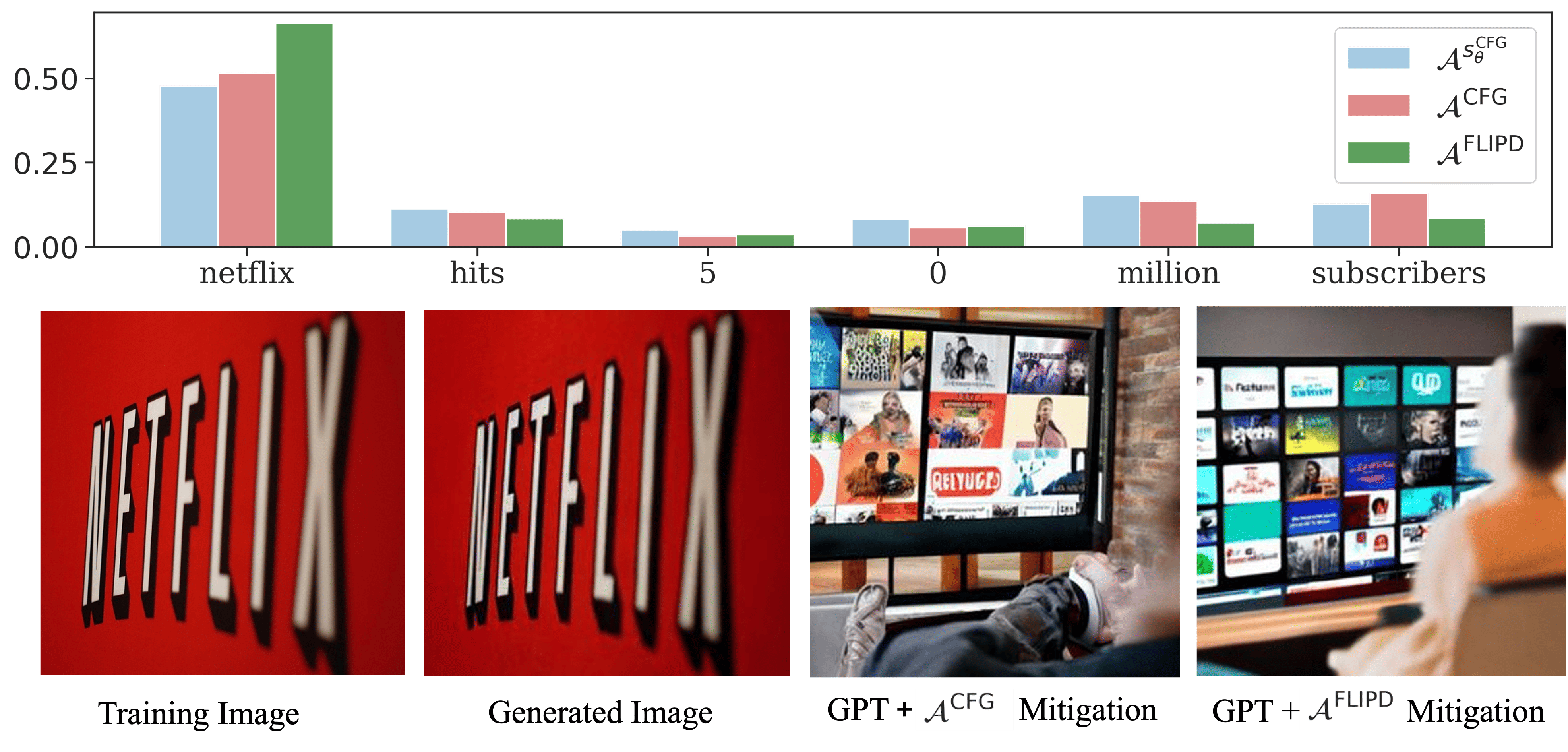
(a) All the methods detect “Netflix” a private trademark driving memorization.

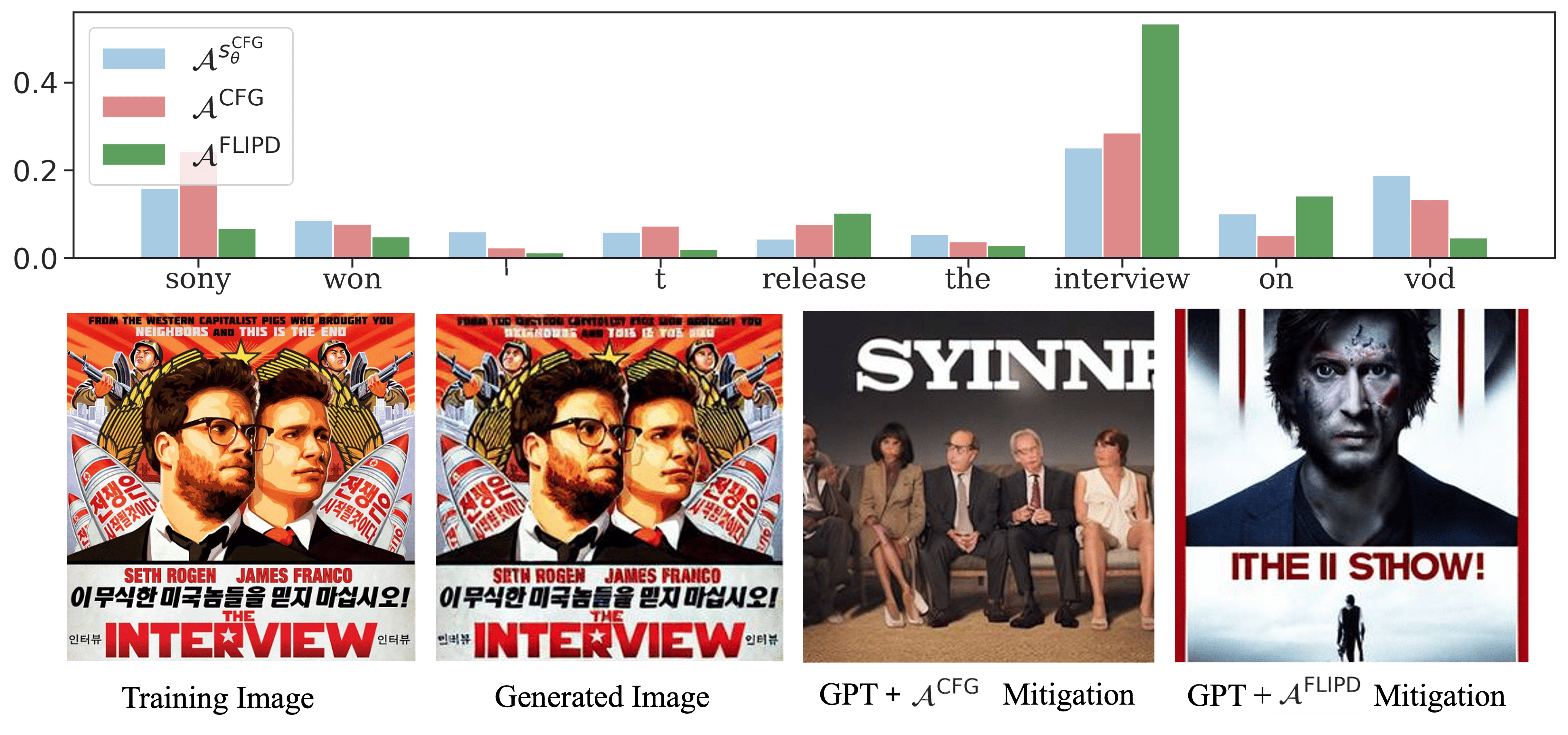
(b) All the methods detect “interview” (the movie title) as the driver for memorization, $\mathcal{A}^{\text{CFG}}$ also detects “Sony” as a significant token.

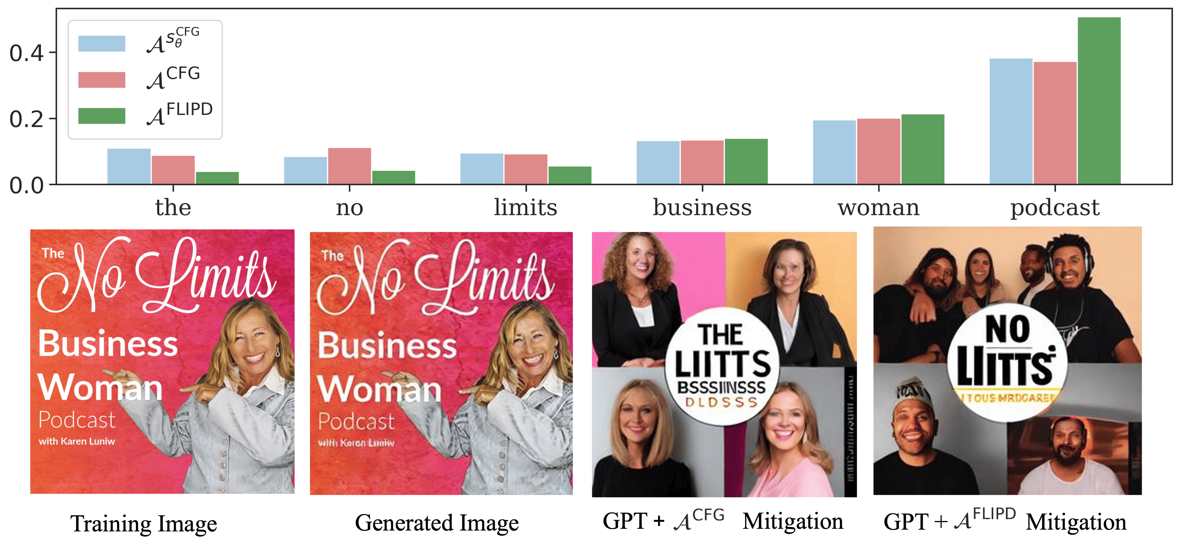
(c) All the methods detect “podcast” as the token driving memorization.

Figure 11: Memorized Stable Diffusion samples with a comparison of token attributions based on three different memorization metrics: the CFG vector norm proposed by Wen et al. (2023), the CFG-adjusted score $s^{\text{CFG}}_{\theta}(x;t,c)$ norm, and the FLIPD estimate for $\text{LID}_{\theta}(\cdot\mid c)$.

We have shown this to be a viable memorization metric, able to detect tokens driving memorization in Figure 11, and behaving comparable to $\mathcal{A}^{\text{CFG}}(c)$, the original metric proposed by Wen et al. (2023). However, a nice property of $\mathcal{A}^{s_{\theta}^{\text{CFG}}}(c)$ is that it can now be linked to MMH: for a memorized prompt where $\text{LID}_{\theta}(\cdot\mid c)$ is small, the score function $\tilde{s}_{\theta}^{\text{CFG}}(\cdot;t,c)$, especially for small $t$, tends to become large, causing the metric in Equation 24 to increase significantly.

Linking to FLIPD

We now propose a more direct proxy for LID based on the FLIPD estimate of $\text{LID}_{\theta}$. Recalling Equation 6, we can define the class-conditional $\text{LID}_{\theta}(\cdot\mid c)$ estimate based on FLIPD as follows, analoguously to Equation 14:

$$\widetilde{\text{FLIPD}}^{\text{CFG}}(\cdot;t,c)=d+\tilde{\sigma}^{2}(t)\cdot\Big{(}\text{tr}\big{(}\nabla\tilde{s}_{\theta}^{\text{CFG}}(\cdot;t,c)\big{)}+\lVert\tilde{s}_{\theta}^{\text{CFG}}(\cdot;t,c)\rVert^{2}\Big{)}.$$ (25)

Noting that $\widetilde{\text{FLIPD}}^{\text{CFG}}(\cdot;t,c)$ has a similar term to Equation 24, we add $d$ and the trace term from Equation 25 into Equation 24, and propose the following MMH-based metric:

$$d+\mathcal{A}^{s_{\theta}^{\text{CFG}}}(c)+\mathbb{E}_{t\sim\mathcal{T}(0,1)}\mathbb{E}_{\tilde{x}_{t}\sim\tilde{p}^{\text{CFG}}_{t}(\cdot\mid c)}\left[\tilde{\sigma}^{2}(t)\cdot\text{tr}\left(\nabla\tilde{s}_{\theta}^{\text{CFG}}\big{(}\tilde{x}_{t};t,c\big{)}\right)\right] =$$ (26)

$$\mathbb{E}_{t\sim\mathcal{T}(0,1)}\mathbb{E}_{\tilde{x}_{t}\sim\tilde{p}^{\text{CFG}}_{t}(\cdot\mid c)}\left[\widetilde{\text{FLIPD}}^{\text{CFG}}(\tilde{x}_{t};t,c)\right] =:\mathcal{A}^{\text{FLIPD}}(c).$$ (27)

Despite the fact that $\mathcal{A}^{\text{FLIPD}}(c)$ can be expressed in terms of $\mathcal{A}^{s_{\theta}^{\text{CFG}}}(c)$, the former indicates memorization when it is small, while the latter indicates memorization when it is large.

Note that while Equation 27 averages FLIPD values over (potentially) all the timesteps $t\in(0,1]$, the theory linking FLIPD and $\text{LID}_{\theta}$ is only rigorously justified when $t\to 0$ (Kamkari et al., 2024b). Hence, we set the scheduling distribution $\mathcal{T}$ such that it primarily samples $t$ close to zero. As such, $\mathcal{A}^{\text{FLIPD}}$ will average FLIPD estimate terms that are closely linked to $\text{LID}_{\theta}(\cdot\mid c)$. Notably, our experiments also revealed that although setting $t$ as small as possible makes sense from a mathematical perspective, the score function, and as a result, FLIPD estimates, become unstable as $t\to 0$ (Pidstrigach, 2022; Kamkari et al., 2024b). Therefore, in practice, we choose $\mathcal{T}$ as a uniform supported on $(0.0,0.2]$; therefore, putting more emphasis on these small $t$ values but at the same time avoiding instabilities in $\mathcal{A}^{\text{FLIPD}}(c)$.

The scheduling is a small, but important distinction between $\mathcal{A}^{\text{FLIPD}}$ on one hand, and $\mathcal{A}^{s_{\theta}^{\text{CFG}}}$ and $\mathcal{A}^{\text{CFG}}$ on the other hand; while $\mathcal{A}^{\text{FLIPD}}$ sets $\mathcal{T}$ as a uniform on $(0.0,0.2]$, $\mathcal{A}^{s_{\theta}^{\text{CFG}}}$ and $\mathcal{A}^{\text{CFG}}$ set $\mathcal{T}$ to a uniform distribution on $(0,1]$, to mirror the setup in Wen et al. (2023).

D.3 Increasing Image Complexity By Optimizing $\mathcal{A}^{\text{FLIPD}}$

Wen et al. (2023) have an experiment where they optimize the prompt (embedding) $c$ directly to minimize ${\color[rgb]{0.8745098039215686,0.5411764705882353,0.5411764705882353}\mathcal{A}^{\text{CFG}}}(c)$, and as a result decrease $\mathcal{A}^{\text{CFG}}(c)$, with the purpose of obviating memorization. Here, we take a similar approach but instead optimize $c$ to maximize $\mathcal{A}^{\text{FLIPD}}(c)$.

In Figure 9, we optimize $c$ with Adam using multiple steps, and as we increase $\mathcal{A}^{\text{FLIPD}}(c)$, we sample images using the prompt embedding which is being optimized. We see that images sampled from these prompts indeed increase in complexity. This is fully consistent with our expectations and understanding of LID. We see, however, that while at a certain range the images are relatively less memorized, the method tends to introduce excessively chaotic textures to artificially increase $\text{LID}_{\theta}(\cdot\mid c)$, often at the expense of the image’s semantic coherence. Despite this, we still find this to be an interesting result and invite future work on using different scheduling approaches for $\mathcal{A}^{\text{FLIPD}}(c)$ that can stabilize the optimization process of $c$.

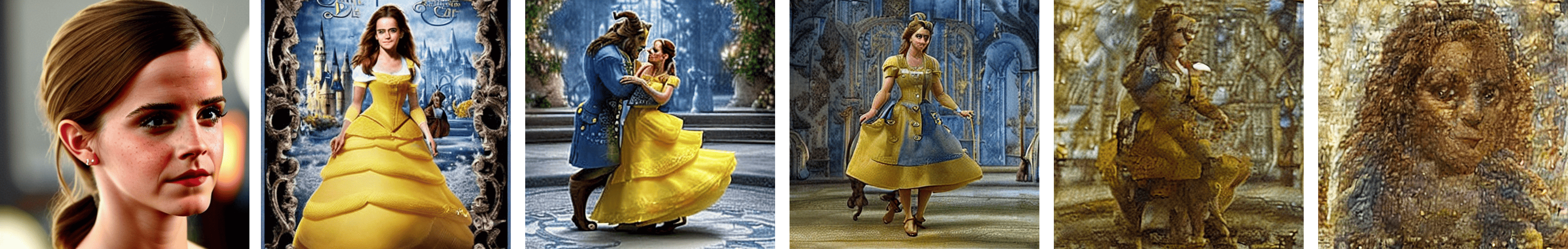
(a) Emma Watson Set to Star Alongside Tom Hanks in Film Adaptation of Dave Eggers’ <i>The Circle</i>

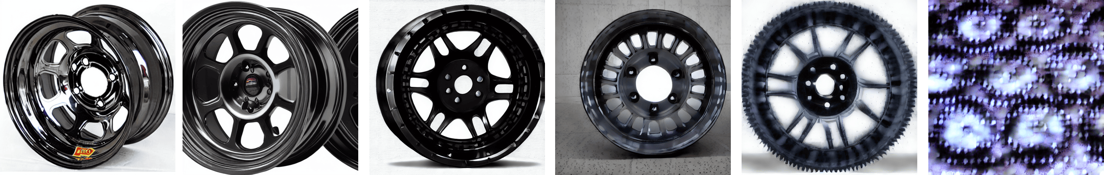
(b) Aero 31-984210BLK 31 Series 13x8 Wheel, Spun 4 on 4-1/4 BP 1 Inch BS

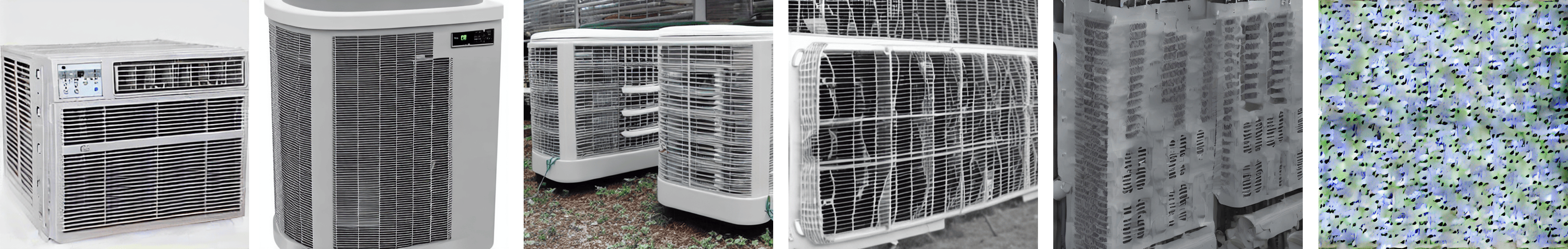
(c) Air Conditioners & Parts

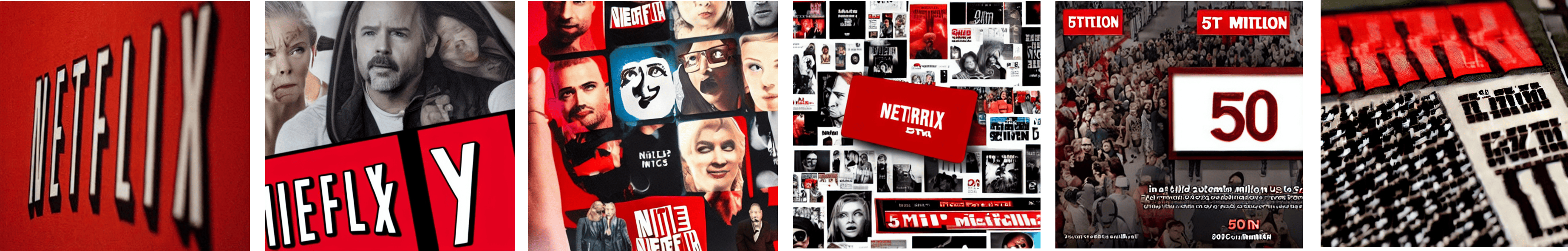
(d) Netflix Hits 50 Million Subscribers

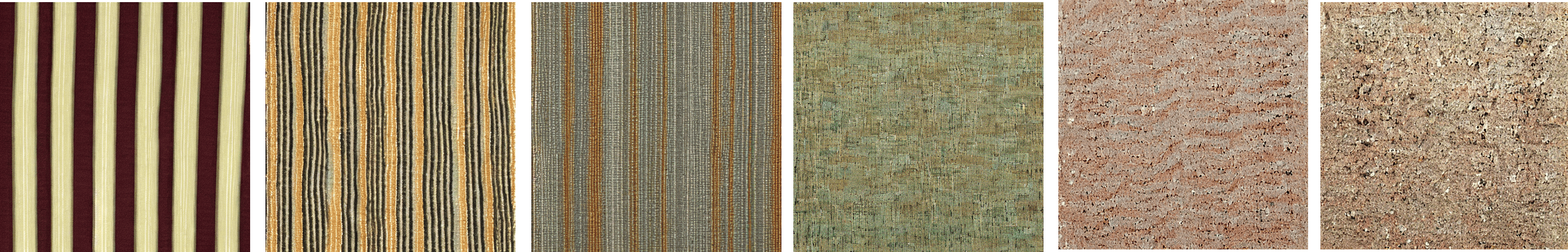
(e) Waterford Sand Silk Stripe Swatch

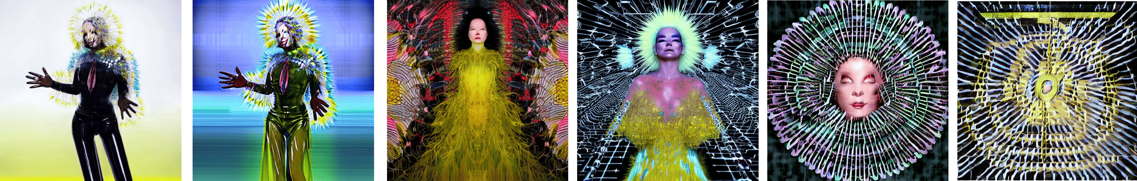
(f) Björk Explains Decision To Pull <i>Vulnicura</i> From Spotify

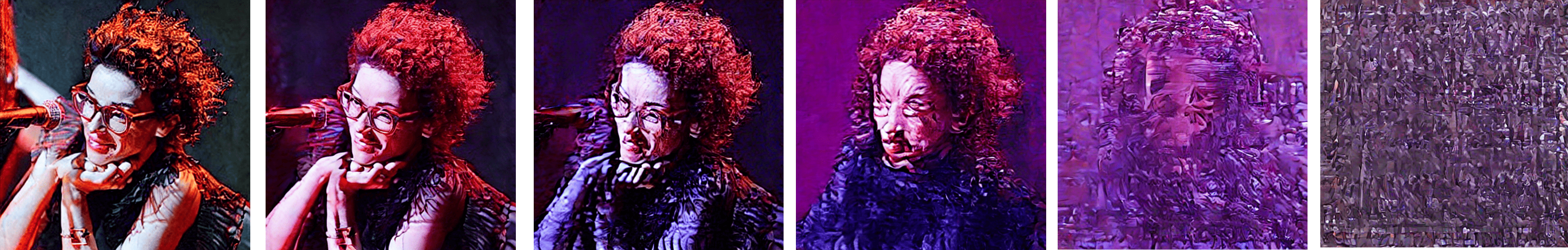
(g) Here’s What You Need to Know About St. Vincent’s Apple Music Radio Show

Figure 9: Samples and their original memorized captions from directly optimizing text conditioning to increase $\mathcal{A}^{\text{FLIPD}}$ and reduce memorization. The images progress through different stages of the optimization process from left to right. While increasing $\text{LID}_{\theta}$ helps reduce memorization, uncontrolled increases often introduce chaotic textures, resulting in unrealistic images.

D.4 Text Perturbation Approaches

GPT-based Perturbations

As outlined in the main text, we sample $k$ tokens without replacement from a categorical distribution obtained by normalizing the token attributions, then use GPT-4 to replace these tokens; this ensures that tokens with the highest attributions are replaced more frequently. After selecting these $k$ tokens, we ask GPT to follow the instructions provided in Box D.4 and use the output of the conversation as the new prompt. This process is repeated five times in our analysis to account for any randomness in the GPT output. It is important to note that these perturbations are designed to preserve the prompt’s semantic structure. To ensure this, the instruction specifically asks GPT not to replace names of places or characters, and to keep the new prompt as semantically close to the original as possible.

Qualitative Comparison

Figure 10 presents a qualitative comparison of our GPT-based perturbations applied to three memorized prompts. We have selected these specific examples to illustrate how the prompt perturbations function in practice. In this case, we set $k=4$ and randomly perturb the tokens based on attributions derived from $\mathcal{A}^{\text{FLIPD}}$. Additionally, Figure 10 includes a column demonstrating the random token addition (RTA) approach proposed by Somepalli et al. (2023a), where $k$ random tokens from the CLIP library are inserted into the prompt. We see that the GPT-based perturbations better preserve the semantic integrity of the text caption, resulting in images that are not memorized and are significantly more coherent.

Memorized Prompt	GPT + $\mathcal{A}^{\text{FLIPD}}$ Mitigation	RTA (Somepalli et al., 2023b)
Talks on the Precepts and Buddhist Ethics	discussions about the precepts and Buddhist principles	Talks mellon dragonball on the villar Precepts and reformed Buddhist Ethics
<i>The Long Dark</i> Gets First Trailer, Steam Early Access	<i>The Long Dark</i> Gets First Trailer; Steam Early Access	barbershop relying <i>The idal Long Dark</i> Gets First Trailer, Steam Early ghorn Access
Sound Advice with John W Doyle	sound guidance with john w doyle	Sound Advice with John payments grill hsfb acadi W Doyle

Figure 10: Comparison of mitigation approaches. The tokens highlighted in red indicate the changes and perturbations made by each approach.

D.5 More Examples of Token Attributions

Appendix E Proofs

We restate each theorem in full formality below along with their proofs.

Throughout this section, we let $P_{*}$ and $P_{\theta}$ be the probability measures of the ground truth data and model, respectively. We assume that the respective supports of $P_{*}$ and $P_{\theta}$ are $\mathcal{M}_{*},\mathcal{M}_{\theta}\subset\mathbb{R}^{d}$, smooth Riemannian submanifolds of the Euclidean space $\mathbb{R}^{d}$ with metrics $g_{*}$ and $g_{\theta}$ respectively. We denote the Riemannian measures on $\mathcal{M}_{*}$ and $\mathcal{M}_{\theta}$ as $\mu_{*}$ and $\mu_{\theta}$, respectively, so that $p_{*}(x)={\textnormal{d}}P_{*}/{\textnormal{d}}\mu_{*}(x)$ and $p_{\theta}(x)={\textnormal{d}}P_{\theta}/{\textnormal{d}}\mu_{\theta}(x)$. As mentioned in Section 2, we take a lax definition of manifold which allows them to vary in dimensionality in different components. A single manifold under our definition is equivalent to a disjoint union of manifolds under the more standard definition.

E.1 3.1

Lemma E.1.

Assume that $p_{*}(x)>0$ for every $x\in\mathcal{M}_{*}$, and let $x_{0}\in\mathcal{M}_{*}$. Then, the following are equivalent:

1. $P_{*}\left(\{x_{0}\}\right)>0$, and

2. $\text{LID}_{*}\left(x_{0}\right)=0$.

Proof.

  

• $(1)\implies(2)$ Assume $P_{*}\left(\{x_{0}\}\right)>0$.

  $$0<P_{*}\left(\{x_{0}\}\right)=\int_{\{x_{0}\}}p_{*}(x){\textnormal{d}}\mu_{*}(x),$$ (28)

  which necessitates $\mu_{*}(\{x_{0}\})>0$. If we had $\text{LID}_{*}(x_{0})>0$ this would incur a contradiction: letting $(U,\phi)$ be a chart around $x_{0}$, then by the definition of $\mu_{*}$,

  $$0<\mu_{*}(\{x_{0}\})=\int_{\phi(\{x_{0}\})}\sqrt{\det(g_{*})}d\lambda,$$ (29)

  where $\lambda$ is the Lebesgue measure on $\mathbb{R}^{\text{LID}_{*}(x_{0})}$ or the counting measure if $\text{LID}_{*}(x_{0})=0$. Due to the singleton domain of integration, positivity of the integral in Equation 29 would be impossible unless $\text{LID}_{*}(x_{0})=0$.

• $(2)\implies(1)$ Suppose $\text{LID}\left(x_{0}\right)=0$. This implies that $\{x_{0}\}$ is an open set in the subspace topology of $\mathcal{M}_{*}$. Since $x_{0}\in\text{supp }\mu_{*}$, any open set containing $x_{0}$ must have positive measure under $\mu_{*}$, so that $\mu_{*}(\{x_{0}\})>0$. Then, since $P_{*}(\{x_{0}\})=p_{*}(x_{0})\mu_{*}(\{x_{0}\})$ and $p_{*}(x_{0})>0$, it follows that $P_{*}(\{x_{0}\})>0$.

∎

Proposition E.2 (Formal Restatement of 3.1).

Assume that $p_{*}(x)>0$ for every $x\in\mathcal{M}_{*}$. Let $\{x_{i}\}_{i=1}^{n}$ be a training dataset drawn independently from $p_{*}(x)$. Then:

1. If duplicates occur in $\{x_{i}\}_{i=1}^{n}$ with positive probability, then they will occur at a point $x_{0}$ such that $\text{LID}_{*}(x_{0})=0$.

2. If $\text{LID}_{*}(x_{0})=0$ for some $x_{0}\in\mathcal{M}_{*}$, then the probability of duplication in $\{x_{i}\}_{i=1}^{n}$ will converge to 1 as $n\to\infty$.

Proof.

  

• $(1)$ Due to E.1, it suffices to show that any duplicates in $\{x_{i}\}_{i=1}^{n}$ must occur at a point $x_{0}$ such that $P_{*}(\{x_{0}\})>0$. It is thus enough to show that if $P_{*}(\{x_{0}\})=0$ for every $x_{0}\in\mathcal{M}_{*}$, then $P_{*}(x_{1}=x_{2})=0$. Assume that $P_{*}(\{x_{0}\})=0$ for every $x_{0}\in\mathcal{M}_{*}$. Since $x_{1}$ and $x_{2}$ are independent, $P_{*}(x_{1}=x_{2})=P_{*}\times P_{*}(D)$, where $D=\{(x,x)\in\mathcal{M}_{*}\times\mathcal{M}_{*}\mid x\in\mathcal{M}_{*}\}$. We then have:

  $$P_{*}\times P_{*}(D) =\int_{D}{\textnormal{d}}P_{*}\times P_{*}(x_{1},x_{2})=\int_{\mathcal{M}_{*}}\int_{\{x_{2}\}}{\textnormal{d}}P_{*}(x_{1}){\textnormal{d}}P_{*}(x_{2})$$ (30)

  $$=\int_{\mathcal{M}_{*}}P_{*}(\{x_{2}\}){\textnormal{d}}P_{*}(x_{2})=0,$$ (31)

  where the second equality follows from Fubini’s theorem (see e.g. Theorem 7.26 in Folland (2013)), and the last equality follows by assumption. This finishes this part of the proof.

• $(2)$ Suppose $\text{LID}_{*}(x_{0})=0$ for some $x_{0}\in\mathcal{M}_{*}$. By E.1, we have $P_{*}\left(\{x_{0}\}\right)>0$. In this case, $P_{*}\left(x_{i}=x_{0}\right)>0$ for all $i\in\{1,\ldots,n\}$, meaning that

  $$P_{*}(x_{i}=x_{j}\text{ for some }1\leq i<j\leq n) \geq P_{*}(x_{i}=x_{j}=x_{0}\text{ for some }1\leq i<j\leq n)$$ (32)

  $$\geq 1-P_{*}(x_{i}\neq x_{0}\text{ for all $i\geq 2$})$$ (33)

  $$=1-P_{*}(x_{2}\neq x_{0})\cdots P_{*}(x_{n}\neq x_{0})$$ (34)

  $$=1-(1-P_{*}(\left\{x_{0}\right\}))^{n-1}$$ (35)

  $$\longrightarrow 1\,,$$ (36)

  where the last line depicts the limiting behaviour as $n\to\infty$.

∎

E.2 3.2

Here we presume the joint distribution of model samples and $k$-dimensional conditioning inputs $(x,c)\in\mathbb{R}^{d+k}$ has support $S\subset\mathbb{R}^{d+k}$ such that $\{x:(x,c)\in S\text{ for some $c\in\mathbb{R}^{k}$}\}=\mathcal{M}_{\theta}$. We define the conditional support of $x$ given $c$ to be $S(c)=\{x:(x,c)\in S\}$.

Proposition E.3 (Formal Restatement of 3.2).

Let $x_{0}\in\mathcal{M}_{\theta}$ and $c\in\mathbb{R}^{k}$. Suppose that $S(c)$ is also a submanifold of $\mathbb{R}^{d}$ and denote its LID at $x_{0}$ by $\text{LID}_{\theta}(x_{0}\mid c)$. We then have

$$\text{LID}_{\theta}(x_{0}\mid c)\leq\text{LID}_{\theta}(x_{0}).$$ (37)

Proof.

If $S(c)$ is a submanifold of $\mathbb{R}^{d}$, then it is also a submanifold of $\mathcal{M}_{\theta}$. The inequality follows directly.∎

E.3 Theorem A.3

Here we show that OD-mem implies data-copying under the definition of Bhattacharjee et al. (2023).

Lemma E.4.

Suppose $(\mathcal{M},g)$ is a $d_{0}$-dimensional smooth Riemannian submanifold of Euclidean space $\mathbb{R}^{d}$. Let $\mu$ be the Riemannian measure of $\mathcal{M}$. If $B_{r}^{d}(x_{0})$ denotes the $d$-dimensional ball of radius $r$ centred at $x_{0}$ in $\mathbb{R}^{d}$, then there exist constants $C_{1}^{\mathcal{M}}>0$ and $C_{2}^{\mathcal{M}}>0$ not depending on $r$ such that for all small enough $r$:

$$C_{1}^{\mathcal{M}}r^{d_{0}}\leq\mu\left(B_{r}^{d}(x_{0})\cap\mathcal{M}\right)\leq C_{2}^{\mathcal{M}}r^{d_{0}}.$$ (38)

Proof.

Without loss of generality, by rotating and translating, we assume $x_{0}=0\in\mathbb{R}^{d}$ and that the tangent plane of $\mathcal{M}$ in $\mathbb{R}^{d}$ at $x_{0}$ is $\mathbb{R}^{d_{0}}\times\{0\}^{d-d_{0}}$.

As $\mathcal{M}$ is smooth, in a neighbourhood $U$ of $x_{0}=0$, $\mathcal{M}$ can be written of a graph of a function $u:U\subset\mathbb{R}^{d_{0}}\rightarrow\mathbb{R}^{d-d_{0}}$, such that $u(0)=0$ and all first derivatives vanish at $0$. Then, for small enough $r>0$, we have

$$B_{r}^{d}(x_{0})\cap\mathcal{M}=\{(z,u(z))\in\mathbb{R}^{d}\mid z\in\mathbb{R}^{d_{0}},\|z\|^{2}+\|u(z)\|^{2}<r^{2}\}.$$ (39)

Let

$$G(r)=\{(z,u(z))\in\mathbb{R}^{d}\mid z\in\mathbb{R}^{d_{0}},\|z\|<r\}$$ (40)

be the graph of $u$ in the open $d_{0}$-ball $B_{r}^{d_{0}}(0)$, and

$$\overline{G(r)}=\{(z,u(z))\in\mathbb{R}^{d}\mid z\in\mathbb{R}^{d_{0}},\|z\|\leq r\}$$ (41)

be the graph of $u$ in the closed $d_{0}$-ball $\overline{B_{r}^{d_{0}}(0)}$. Note that both are defined when $u$ is defined, i.e. small enough $r$, and are subset of $\mathcal{M}$. Then it is clear that we have

$$B_{r}^{d}(x_{0})\cap\mathcal{M}\subseteq G(r).$$ (42)

Now, consider the function $v(z)=\frac{\|u(z)\|}{\|z\|}$. Note that $v(z)$ is continuous everywhere in $B_{r}^{d_{0}}(0)\setminus\{0\}$. Since $u$ and its derivatives vanish at $z=0$, from the definition, we have $\lim_{z\rightarrow 0}v(z)=0$ as well. Thus $v(z)$ can be extended to a continuous function in $B_{r}^{d_{0}}(0)$. Fix $R>0$, and let $K$ be the maximum of $v$ over $\overline{B_{R}^{d_{0}}}$. Then, if $\|z\|<ar$ where $a=\frac{1}{\sqrt{1+K^{2}}}$, we have

$$\|z\|^{2}+\|u(z)\|^{2}=\|z\|^{2}(1+v(z)^{2})\leq\|z\|^{2}(1+K^{2})<r^{2}.$$ (43)

This shows that $G(ar)\subseteq B_{r}^{d}(x_{0})\cap\mathcal{M}$ for $0<r<R$. Thus we have

$$\mu(G(ar))\leq\mu(B_{r}^{d}(x_{0})\cap\mathcal{M})\leq\mu(G(r)).$$ (44)

Let $K_{1}$ and $K_{2}$ be the minimum and maximum of $\sqrt{\det g}$ over $\overline{B_{r}^{d_{0}}(0)}$, respectively. Then we have

$$\mu(G(r))=\int_{B_{r}^{d_{0}}(0)}\sqrt{\det g}\,{\textnormal{d}}z\leq\int_{B_{r}^{d_{0}}(0)}K_{2}{\textnormal{d}}z=K_{2}V_{d_{0}}r^{d_{0}}$$ (45)

and

$$\mu(G(r))=\int_{B_{r}^{d_{0}}(0)}\sqrt{\det g}\,{\textnormal{d}}z\geq\int_{B_{r}^{d_{0}}(0)}K_{1}{\textnormal{d}}z=K_{1}V_{d_{0}}r^{d_{0}},$$ (46)

where $V_{d_{0}}$ is the Euclidean volume of the unit $d_{0}$-ball. Combining the above results, we have

$$K_{1}V_{d_{0}}a^{d_{0}}r^{d_{0}}\leq\mu(G(ar))\leq\mu(B_{r}^{d}(x_{0})\cap\mathcal{M})\leq\mu(G(r))\leq K_{2}V_{d_{0}}r^{d_{0}},$$ (47)

which finishes the proof with $C_{1}^{\mathcal{M}}=K_{1}V_{d_{0}}a^{d_{0}}$ and $C_{2}^{\mathcal{M}}=K_{2}V_{d_{0}}$. ∎

Theorem E.5 (Formal Restatement of Theorem A.3).

Assume that $p_{*}(x)$ and $p_{\theta}(x)$ are continuous and that $p_{\theta}(x)$ is strictly positive. Let $x_{0}\in\mathcal{M}_{\theta}\cap\mathcal{M}_{*}$ and let $p_{\theta}(x)$ be a model undergoing OD-mem at $x_{0}$, i.e. $0\leq\text{LID}_{\theta}(x_{0})<\text{LID}_{*}(x_{0})$. Then for any $\lambda>1$ and $0<\gamma<1$, there exists a radius $r_{0}$ such that any $x\in B_{r_{0}}^{d}(x_{0})$ is a $(\lambda,\gamma)$-copy of $x_{0}$ according to A.1, and if $\{x_{j}\}_{j=1}^{m}$ is generated independently from $p_{\theta}(x)$, then the probability of $(\lambda,\gamma)$-copying $x_{0}$ converges to $1$ as $m\to\infty$.

Proof.

For an arbitrary value of $r>0$, we have that

$$P_{\theta}(B_{r}^{d}(x_{0}))\geq\mu_{\theta}(B_{r}^{d}(x_{0})\cap\mathcal{M}_{\theta})\inf_{x\in B_{r}^{d}(x_{0})\cap\mathcal{M}_{\theta}}p_{\theta}(x)$$ (48)

and similarly,

$$P_{*}(B_{r}^{d}(x_{0}))\leq\mu_{*}(B_{r}^{d}(x_{0})\cap\mathcal{M}_{*})\sup_{x\in B_{r}^{d}(x_{0}))\cap\mathcal{M}_{*}}p_{*}(x).$$ (49)

Using E.4,

$$\frac{P_{*}(B_{r}^{d}(x_{0}))}{P_{\theta}(B_{r}^{d}(x_{0}))} \leq\frac{\mu_{*}(B_{r}^{d}(x_{0})\cap\mathcal{M}_{*})}{\mu_{\theta}(B_{r}^{d}(x_{0})\cap\mathcal{M}_{\theta})}\cdot\frac{\sup_{x\in B_{r}^{d}(x_{0})\cap\mathcal{M}_{*}}p_{*}(x)}{\inf_{x\in B_{r}^{d}(x_{0})\cap\mathcal{M}_{\theta}}p_{\theta}(x)}$$ (50)

$$\leq\dfrac{C_{2}^{\mathcal{M}_{*}}}{C_{1}^{\mathcal{M}_{\theta}}}r^{\text{LID}_{*}(x_{0})-\text{LID}_{\theta}(x_{0})}\frac{\sup_{x\in B_{r}^{d}(x_{0})\cap\mathcal{M}_{*}}p_{*}(x)}{\inf_{x\in B_{r}^{d}(x_{0})\cap\mathcal{M}_{\theta}}p_{\theta}(x)}.$$ (51)

Note that by continuity and positivity of $p_{\theta}(x)$, $\inf_{x\in B_{r}^{d}(x_{0})\cap\mathcal{M}_{\theta}}p_{\theta}(x)$ is bounded away from $0$ as $r\rightarrow 0$, and by continuity of $p_{*}(x)$, $\sup_{x\in B_{r}^{d}(x_{0})\cap\mathcal{M}_{*}}$ is bounded. In turn, since by assumption $\text{LID}_{*}(x_{0})>\text{LID}_{\theta}(x_{0})$, Equation 51 converges to $0$ as $r\rightarrow 0$. As a result, there exists some ${r_{0}}$ sufficiently small enough for both

$$\frac{P_{*}(B_{r_{0}}^{d}(x_{0}))}{P_{\theta}(B_{r_{0}}^{d}(x_{0}))}\leq\frac{1}{\lambda}$$ (52)

and

$$P_{*}(B_{r_{0}}^{d}(x_{0}))\leq\gamma$$ (53)

to be true (the latter arising from the fact that $P_{*}(B_{r}^{d}(x_{0}))\to 0$ as $r\to 0$, which follows from $P_{*}$ being absolutely continuous with respect to $\mu_{*}$ and $\mu_{*}$ not assigning positive measure to singletons because $\text{LID}_{*}(x_{0})>0$).

Thus, any $x\in B_{r_{0}}^{d}(x_{0})$ is a $(\lambda,\gamma)$-copy of $x_{0}$. Since $B_{r_{0}}^{d}(x_{0})\cap\mathcal{M}_{\theta}$ contains an open set in the subspace topology of $\mathcal{M}_{\theta}$, it follows that $\mu_{\theta}(B_{r_{0}}^{d}(x_{0})\cap\mathcal{M}_{\theta})>0$. Then, since $p_{\theta}(x)$ is strictly positive, $P_{\theta}(B_{r_{0}}^{d}(x_{0}))>0$, so that

$$P_{\theta}(x_{j} \text{ is a $(\lambda,\gamma)$-copy of $x_{0}$ for some }1\leq j\leq m)$$ (54)

$$=1-P_{\theta}(x_{j}\text{ is not a $(\lambda,\gamma)$-copy of $x_{0}$ for every }1\leq j\leq m)$$ (55)

$$=1-P_{\theta}(x_{1}\text{ is not a $(\lambda,\gamma)$-copy of $x_{0}$})\cdots P_{\theta}(x_{m}\text{ is not a $(\lambda,\gamma)$-copy of $x_{0}$})$$ (56)

$$\geq 1-(1-P_{\theta}(B_{r_{0}}^{d}(x_{0})))^{m}$$ (57)

converges to $1$ as $m\to\infty$.

∎

References

- Akbar et al. (2023) Muhammad Usman Akbar, Wuhao Wang, and Anders Eklund. Beware of diffusion models for synthesizing medical images–A comparison with GANs in terms of memorizing brain MRI and chest x-ray images. arXiv:2305.07644, 2023.
- Bai et al. (2021) Ching-Yuan Bai, Hsuan-Tien Lin, Colin Raffel, and Wendy Chi-wen Kan. On training sample memorization: Lessons from benchmarking generative modeling with a large-scale competition. In Proceedings of the 27th ACM SIGKDD Conference on Knowledge Discovery & Data Mining, pp. 2534–2542, 2021.
- Bengio et al. (2013) Yoshua Bengio, Aaron Courville, and Pascal Vincent. Representation learning: A review and new perspectives. IEEE Transactions on Pattern Analysis and Machine Intelligence, 35(8):1798–1828, 2013.
- Bhattacharjee et al. (2023) Robi Bhattacharjee, Sanjoy Dasgupta, and Kamalika Chaudhuri. Data-copying in generative models: a formal framework. In International Conference on Machine Learning, 2023.
- Bradski (2000) G. Bradski. The OpenCV Library. Dr. Dobb’s Journal of Software Tools, 2000.
- Brown et al. (2023) Bradley CA Brown, Anthony L Caterini, Brendan Leigh Ross, Jesse C Cresswell, and Gabriel Loaiza-Ganem. Verifying the union of manifolds hypothesis for image data. In International Conference on Learning Representations, 2023.
- Carlini et al. (2022) Nicholas Carlini, Daphne Ippolito, Matthew Jagielski, Katherine Lee, Florian Tramer, and Chiyuan Zhang. Quantifying memorization across neural language models. In The Eleventh International Conference on Learning Representations, 2022.
- Carlini et al. (2023) Nicolas Carlini, Jamie Hayes, Milad Nasr, Matthew Jagielski, Vikash Sehwag, Florian Tramer, Borja Balle, Daphne Ippolito, and Eric Wallace. Extracting training data from diffusion models. In 32nd USENIX Security Symposium, pp. 5253–5270, 2023.
- Chen et al. (2024) Chen Chen, Daochang Liu, and Chang Xu. Towards memorization-free diffusion models. In Proceedings of the IEEE/CVF Conference on Computer Vision and Pattern Recognition, 2024.
- Dai & Wipf (2019) Bin Dai and David Wipf. Diagnosing and enhancing VAE models. In International Conference on Learning Representations, 2019.
- Daras et al. (2024) Giannis Daras, Alex Dimakis, and Constantinos Costis Daskalakis. Consistent Diffusion Meets Tweedie: Training Exact Ambient Diffusion Models with Noisy Data. In International Conference on Machine Learning, 2024.
- Dinh et al. (2014) Laurent Dinh, David Krueger, and Yoshua Bengio. NICE: Non-linear independent components estimation. arXiv:1410.8516, 2014.
- Feng et al. (2021) Qianli Feng, Chenqi Guo, Fabian Benitez-Quiroz, and Aleix M Martinez. When do GANs replicate? on the choice of dataset size. In Proceedings of the IEEE/CVF International Conference on Computer Vision, pp. 6701–6710, 2021.
- Folland (2013) G.B. Folland. Real Analysis: Modern Techniques and Their Applications. Wiley, 2013.
- Fukunaga & Olsen (1971) Keinosuke Fukunaga and David R Olsen. An algorithm for finding intrinsic dimensionality of data. IEEE Transactions on Computers, 100(2):176–183, 1971.
- Goodfellow et al. (2014) Ian Goodfellow, Jean Pouget-Abadie, Mehdi Mirza, Bing Xu, David Warde-Farley, Sherjil Ozair, Aaron Courville, and Yoshua Bengio. Generative adversarial nets. In Advances in Neural Information Processing Systems, volume 27, 2014.
- Gu et al. (2023) Xiangming Gu, Chao Du, Tianyu Pang, Chongxuan Li, Min Lin, and Ye Wang. On memorization in diffusion models. arXiv:2310.02664, 2023.
- Hintersdorf et al. (2024) Dominik Hintersdorf, Lukas Struppek, Kristian Kersting, Adam Dziedzic, and Franziska Boenisch. Finding NeMo: Localizing Neurons Responsible For Memorization in Diffusion Models. arXiv:2406.02366, 2024.
- Ho et al. (2020) Jonathan Ho, Ajay Jain, and Pieter Abbeel. Denoising diffusion probabilistic models. In Advances in Neural Information Processing Systems, volume 33, 2020.
- Horvat & Pfister (2022) Christian Horvat and Jean-Pascal Pfister. Intrinsic dimensionality estimation using normalizing flows. In Advances in Neural Information Processing Systems, 2022.
- Horvat & Pfister (2024) Christian Horvat and Jean-Pascal Pfister. On gauge freedom, conservativity and intrinsic dimensionality estimation in diffusion models. In The Twelfth International Conference on Learning Representations, 2024.
- Hugging Face (2024) Hugging Face. Tuxemon. https://huggingface.co/datasets/diffusers/tuxemon, 2024.
- Humayun et al. (2024) Ahmed Imtiaz Humayun, Ibtihel Amara, Candice Schumann, Golnoosh Farnadi, Negar Rostamzadeh, and Mohammad Havaei. Understanding the local geometry of generative model manifolds. arXiv e-prints, pp. arXiv–2408, 2024.
- Hutchinson (1989) Michael F Hutchinson. A stochastic estimator of the trace of the influence matrix for laplacian smoothing splines. Communications in Statistics-Simulation and Computation, 18(3):1059–1076, 1989.
- Kadkhodaie et al. (2024) Zahra Kadkhodaie, Florentin Guth, Eero P Simoncelli, and Stéphane Mallat. Generalization in diffusion models arises from geometry-adaptive harmonic representation. In International Conference on Learning Representations, 2024.
- Kamkari et al. (2024a) Hamidreza Kamkari, Brendan Leigh Ross, Jesse C Cresswell, Anthony L Caterini, Rahul G Krishnan, and Gabriel Loaiza-Ganem. A geometric explanation of the likelihood OOD detection paradox. In International Conference on Machine Learning, 2024a.
- Kamkari et al. (2024b) Hamidreza Kamkari, Brendan Leigh Ross, Rasa Hosseinzadeh, Jesse C Cresswell, and Gabriel Loaiza-Ganem. A geometric view of data complexity: Efficient local intrinsic dimension estimation with diffusion models. In Advances in Neural Information Processing Systems, volume 37, 2024b.
- Karras et al. (2019) Tero Karras, Samuli Laine, and Timo Aila. A style-based generator architecture for generative adversarial networks. In Proceedings of the IEEE/CVF conference on Computer Vision and Pattern Recognition, pp. 4401–4410, 2019.
- Karras et al. (2020) Tero Karras, Miika Aittala, Janne Hellsten, Samuli Laine, Jaakko Lehtinen, and Timo Aila. Training generative adversarial networks with limited data. In Advances in Neural Information Processing Systems, volume 33, 2020.
- Kingma & Welling (2014) Diederik P Kingma and Max Welling. Auto-encoding variational Bayes. In International Conference on Learning Representations, 2014.
- Krizhevsky & Hinton (2009) Alex Krizhevsky and Geoffrey Hinton. Learning multiple layers of features from tiny images. Technical Report, 2009.
- Lee (2012) John M Lee. Introduction to Smooth Manifolds. Springer New York, 2012.
- Levina & Bickel (2004) Elizaveta Levina and Peter Bickel. Maximum likelihood estimation of intrinsic dimension. In Advances in Neural Information Processing Systems, 2004.
- Li et al. (2023) Puheng Li, Zhong Li, Huishuai Zhang, and Jiang Bian. On the generalization properties of diffusion models. Advances in Neural Information Processing Systems, 36, 2023.
- Li et al. (2024) Sixu Li, Shi Chen, and Qin Li. A good score does not lead to a good generative model. arXiv:2401.04856, 2024.
- Lin et al. (2014) Tsung-Yi Lin, Michael Maire, Serge Belongie, James Hays, Pietro Perona, Deva Ramanan, Piotr Dollár, and C Lawrence Zitnick. Microsoft coco: Common objects in context. In Computer Vision–ECCV 2014: 13th European Conference, Zurich, Switzerland, September 6-12, 2014, Proceedings, Part V 13, pp. 740–755. Springer, 2014.
- Loaiza-Ganem et al. (2022) Gabriel Loaiza-Ganem, Brendan Leigh Ross, Jesse C Cresswell, and Anthony L. Caterini. Diagnosing and fixing manifold overfitting in deep generative models. Transactions on Machine Learning Research, 2022.
- Loaiza-Ganem et al. (2024) Gabriel Loaiza-Ganem, Brendan Leigh Ross, Rasa Hosseinzadeh, Anthony L Caterini, and Jesse C Cresswell. Deep generative models through the lens of the manifold hypothesis: A survey and new connections. Transactions on Machine Learning Research, 2024.
- Lu et al. (2023) Yubin Lu, Zhongjian Wang, and Guillaume Bal. Mathematical analysis of singularities in the diffusion model under the submanifold assumption. arXiv:2301.07882, 2023.
- Meehan et al. (2020) Casey Meehan, Kamalika Chaudhuri, and Sanjoy Dasgupta. A non-parametric test to detect data-copying in generative models. In International Conference on Artificial Intelligence and Statistics, 2020.
- Nagarajan et al. (2018) Vaishnavh Nagarajan, Colin Raffel, and Ian J Goodfellow. Theoretical insights into memorization in gans. In Neural Information Processing Systems Workshop, volume 1, pp. 3, 2018.
- Nichol et al. (2022) Alex Nichol, Aditya Ramesh, Pamela Mishkin, Prafulla Dariwal, Joanne Jang, and Mark Chen. DALLE 2 Pre-Training Mitigations, June 2022. URL https://openai.com/blog/dall-e-2-pre-training-mitigations/.
- Nichol & Dhariwal (2021) Alexander Quinn Nichol and Prafulla Dhariwal. Improved denoising diffusion probabilistic models. In International conference on machine learning, pp. 8162–8171. PMLR, 2021.
- OpenAI (2023) OpenAI. Gpt-4. https://openai.com, 2023. GPT-4o.
- Orrick (2023) William H. Orrick. Andersen v. Stability AI Ltd., 2023. URL https://casetext.com/case/andersen-v-stability-ai-ltd.
- Pidstrigach (2022) Jakiw Pidstrigach. Score-based generative models detect manifolds. In Advances in Neural Information Processing Systems, 2022.
- Pizzi et al. (2022) Ed Pizzi, Sreya Dutta Roy, Sugosh Nagavara Ravindra, Priya Goyal, and Matthijs Douze. A self-supervised descriptor for image copy detection. In Proceedings of the IEEE/CVF Conference on Computer Vision and Pattern Recognition, pp. 14532–14542, 2022.
- Radford et al. (2021) Alec Radford, Jong Wook Kim, Chris Hallacy, Aditya Ramesh, Gabriel Goh, Sandhini Agarwal, Girish Sastry, Amanda Askell, Pamela Mishkin, Jack Clark, et al. Learning transferable visual models from natural language supervision. In International conference on machine learning, pp. 8748–8763. PMLR, 2021.
- Rezende et al. (2014) Danilo Jimenez Rezende, Shakir Mohamed, and Daan Wierstra. Stochastic backpropagation and approximate inference in deep generative models. In International Conference on Machine Learning, pp. 1278–1286, 2014.
- Rombach et al. (2022) Robin Rombach, Andreas Blattmann, Dominik Lorenz, Patrick Esser, and Björn Ommer. High-resolution image synthesis with latent diffusion models. In Proceedings of the IEEE/CVF Conference on Computer Vision and Pattern Recognition, pp. 10684–10695, 2022.
- Ross et al. (2023) Brendan Leigh Ross, Gabriel Loaiza-Ganem, Anthony L Caterini, and Jesse C Cresswell. Neural implicit manifold learning for topology-aware generative modelling. Transactions on Machine Learning Research, 2023.
- Schuhmann et al. (2022) Christoph Schuhmann, Romain Beaumont, Richard Vencu, Cade Gordon, Ross Wightman, Mehdi Cherti, Theo Coombes, Aarush Katta, Clayton Mullis, Mitchell Wortsman, Patrick Schramowski, Srivatsa Kundurthy, Katherine Crowson, Ludwig Schmidt, Robert Kaczmarczyk, and Jenia Jitsev. LAION-5B: An open large-scale dataset for training next generation image-text models. In Advances in Neural Information Processing Systems, volume 35, 2022.
- Sohl-Dickstein et al. (2015) Jascha Sohl-Dickstein, Eric Weiss, Niru Maheswaranathan, and Surya Ganguli. Deep unsupervised learning using nonequilibrium thermodynamics. In International Conference on Machine Learning, pp. 2256–2265, 2015.
- Somepalli et al. (2023a) Gowthami Somepalli, Vasu Singla, Micah Goldblum, Jonas Geiping, and Tom Goldstein. Diffusion art or digital forgery? investigating data replication in diffusion models. In Proceedings of the IEEE/CVF Conference on Computer Vision and Pattern Recognition, 2023a.
- Somepalli et al. (2023b) Gowthami Somepalli, Vasu Singla, Micah Goldblum, Jonas Geiping, and Tom Goldstein. Understanding and mitigating copying in diffusion models. In Advances in Neural Information Processing Systems, volume 36, 2023b.
- Song et al. (2020) Jiaming Song, Chenlin Meng, and Stefano Ermon. Denoising diffusion implicit models. arXiv:2010.02502, October 2020. URL https://arxiv.org/abs/2010.02502.
- Song et al. (2021) Yang Song, Jascha Sohl-Dickstein, Diederik P Kingma, Abhishek Kumar, Stefano Ermon, and Ben Poole. Score-based generative modeling through stochastic differential equations. In International Conference on Learning Representations, 2021.
- Stanczuk et al. (2024) Jan Pawel Stanczuk, Georgios Batzolis, Teo Deveney, and Carola-Bibiane Schönlieb. Diffusion models encode the intrinsic dimension of data manifolds. In Proceedings of the 41st International Conference on Machine Learning, 2024.
- Stein et al. (2023) George Stein, Jesse C Cresswell, Rasa Hosseinzadeh, Yi Sui, Brendan Ross, Valentin Villecroze, Zhaoyan Liu, Anthony L Caterini, J Eric T Taylor, and Gabriel Loaiza-Ganem. Exposing flaws of generative model evaluation metrics and their unfair treatment of diffusion models. In Advances in Neural Information Processing Systems, volume 36, 2023.
- Tempczyk et al. (2022) Piotr Tempczyk, Rafał Michaluk, Lukasz Garncarek, Przemysław Spurek, Jacek Tabor, and Adam Golinski. LIDL: Local intrinsic dimension estimation using approximate likelihood. In International Conference on Machine Learning, pp. 21205–21231, 2022.
- Tuxemon Project (2024) Tuxemon Project. Tuxemon, 2024. URL https://tuxemon.org/.
- Vahdat et al. (2021) Arash Vahdat, Karsten Kreis, and Jan Kautz. Score-based generative modeling in latent space. In Advances in Neural Information Processing Systems, volume 34, 2021.
- Vyas et al. (2023) Nikhil Vyas, Sham M Kakade, and Boaz Barak. On provable copyright protection for generative models. In International Conference on Machine Learning, pp. 35277–35299. PMLR, 2023.
- Webster (2023) Ryan Webster. A reproducible extraction of training images from diffusion models. arXiv:2305.08694, 2023.
- Webster et al. (2021) Ryan Webster, Julien Rabin, Loic Simon, and Frederic Jurie. This person (probably) exists. Identity membership attacks against GAN generated faces. arXiv:2107.06018, 2021.
- Wen et al. (2023) Yuxin Wen, Yuchen Liu, Chen Chen, and Lingjuan Lyu. Detecting, explaining, and mitigating memorization in diffusion models. In The Twelfth International Conference on Learning Representations, 2023.
- Yi et al. (2023) Mingyang Yi, Jiacheng Sun, and Zhenguo Li. On the generalization of diffusion model. arXiv:2305.14712, 2023.
- Yoon et al. (2023) TaeHo Yoon, Joo Young Choi, Sehyun Kwon, and Ernest K Ryu. Diffusion probabilistic models generalize when they fail to memorize. In ICML 2023 Workshop on Structured Probabilistic Inference & Generative Modeling, 2023.
- Zheng et al. (2022) Yijia Zheng, Tong He, Yixuan Qiu, and David P Wipf. Learning manifold dimensions with conditional variational autoencoders. In Advances in Neural Information Processing Systems, volume 35, 2022.