Derivative-Free Optimization via Finite Difference Approximation: An Experimental Study

Abstract

Derivative-free optimization (DFO) is vital in solving complex optimization problems where only noisy function evaluations are available through an oracle. Within this domain, DFO via finite difference (FD) approximation has emerged as a powerful method. Two classical approaches are the Kiefer-Wolfowitz (KW) and simultaneous perturbation stochastic approximation (SPSA) algorithms, which estimate gradients using just two samples in each iteration to conserve samples. However, this approach yields imprecise gradient estimators, necessitating diminishing step sizes to ensure convergence, often resulting in slow optimization progress. In contrast, FD estimators constructed from batch samples approximate gradients more accurately. While gradient descent algorithms using batch-based FD estimators achieve more precise results in each iteration, they require more samples and permit fewer iterations. This raises a fundamental question: which approach is more effective—KW-style methods or DFO with batch-based FD estimators? This paper conducts a comprehensive experimental comparison among these approaches, examining the fundamental trade-off between gradient estimation accuracy and iteration steps. Through extensive experiments in both low-dimensional and high-dimensional settings, we demonstrate a surprising finding: when an efficient batch-based FD estimator is applied, its corresponding gradient descent algorithm generally shows better performance compared to classical KW and SPSA algorithms in our tested scenarios.
Key words: DRO, SPSA, KW, Cor-CFD

1 Introduction

DFO addresses complex optimization problems where only noisy function evaluations are available through an oracle or black-box interface. This optimization framework has broad applications across diverse fields, including engineering design, black-box system optimization, and hyperparameter tuning in machine learning. For example, Google has developed an internal service, Google Vizier, based on DFO methods to optimize many machine learning models and complex systems (Golovin et al., 2017). This service has executed millions of optimizations, accelerating numerous research and production systems at Google (Song et al., 2024). For a comprehensive overview of DFO, refer to Larson et al. (2019). In this paper, we focus on DFO via FD approximation, an important topic in simulation optimization (see, e.g., Chau and Fu, 2015; Fu, 2015; Hu and Fu, 2024), which has recently attracted substantial attention in machine learning (see, e.g., Shi et al., 2023; Xuan, 2023).

FD approximation is a classical gradient estimation approach when the closed-form derivatives of functions are unavailable. This method involves generating samples at perturbed inputs. Fox and Glynn (1989) and Zazanis and Suri (1993) examine a batch-based FD estimator that uses a batch of independent and identically distributed (i.i.d.) samples generated at perturbed inputs. Specifically, they provide the theoretical optimal perturbation size given the batch size. However, unknown constants in the optimal perturbation size present a challenge for practical use of the batch-based FD estimator. Thus, the estimator must either assume known constants or tune them as hyperparameters. To overcome this issue, Li and Lam (2020) provide a two-stage procedure. In the first stage, the optimal perturbation is estimated by some pilot samples; in the second stage, the FD estimator is constructed by additional samples generated at the estimated perturbation. Recently, Liang et al. (2024) propose a novel FD method called correlation-induced FD (Cor-FD) to address the limitations of conventional FD methods. Unlike conventional FD methods that assume known optimal perturbation parameters, Cor-FD employs a sample-driven framework, dynamically estimating the optimal perturbation by combining bootstrap and regression techniques. The method’s distinctive feature lies in its ability to leverage all available simulation samples by transforming them according to the estimated optimal perturbation, thereby generating correlated samples that enhance estimation accuracy. Also, Liang et al. (2024) demonstrate that their proposed Cor-FD estimator possesses a reduced variance, and in some cases a reduced bias, compared to the conventional optimal FD estimator.

In simulation optimization, DFO via FD can track back to Kiefer and Wolfowitz (1952), where they originally design a one-dimensional optimization problem and propose a gradient decent method that replaces the gradient with an FD estimator using only two function evaluations per iteration. This is called the KW algorithm. In the high-dimensional setting, Spall (1992) propose a more efficient alternative, known as the SPSA algorithm. This algorithm maintains the two-function-evaluation requirement regardless of dimensionality by employing a random perturbation vector, making it particularly suitable for large-scale optimization problems. To ensure algorithm convergence, both the step size and perturbation size must approach zero as iterations progress to infinity, and they must satisfy certain relationships. Notably, the performance of the KW and SPSA algorithms is sensitive to both step size and perturbation size, which must therefore be selected carefully.

Another line of research in DFO via FD sets a fixed perturbation size, with no requirement for the step size to tend to zero. As a result, the algorithm’s output converges to a neighborhood around the optimal solutions (Berahas et al., 2019; Shi et al., 2023; Bollapragada et al., 2024). Specifically, Shi et al. (2023) strongly recommends solving DFO problems via FD due to its natural compatibility with parallel computing. Moreover, it can be built based on the existing software, thereby avoiding the need to redesign the current DFO algorithms to handle general problems.

Most algorithms about DFO via FD apply the FD estimator with only two function evaluations per iteration to conserve samples during multiple iterations. Although this approach seems computationally efficient, it encounters several fundamental limitations. The gradient estimates obtained from such minimal sampling often suffer from significant inaccuracies, arising from the choice of perturbation parameters and inherent simulation noise. To ensure convergence under such imprecise gradient estimates, these methods must resort to diminishing step sizes, which often results in slow convergence rates and reduced practical efficiency. Batch-based FD estimator seems sample-consuming, yet can approximate the gradient more accurately, providing a more accurate direction of gradient descent. This enhanced precision in gradient estimation enables the use of constant step sizes throughout the optimization process, eliminating the necessity of diminishing step lengths that are typically required by less accurate estimators.

In this paper, we apply the correlation-induced central FD (Cor-CFD) method to solve DFO problems and provide a numerical comparison with the aforementioned two classical algorithms: KW and SPSA, under various experimental settings, including both low-dimensional and high-dimensional test problems with varying levels of noise and different function landscapes. In low-dimensional problems, the numerical results show that Cor-CFD maintains stable convergence behavior, while the KW algorithm often exhibits oscillation‌ in its optimization trajectory. The Cor-CFD method generally outperforms KW in terms of solution quality. When tackling high-dimensional problems, Cor-CFD demonstrates substantially faster convergence rates compared to SPSA.

The rest of this paper is organized as follows. Section 2 lays down the gradient-based optimization framework, introducing two mainstream approaches for gradient estimation in stochastic environments: methods using minimal samples per iteration (KW and SPSA) and method employing larger batch sizes for more accurate gradient estimation (Cor-CFD). Section 3 validates the proposed method through numerical experiments, comparing it to the KW algorithm in one-dimensional cases and the SPSA algorithm in high-dimensional case. The results highlight the batch-based method’s superior performance in both convergence stability and computational efficiency, with Section 4 summarizing findings and future directions.

2 Stochastic Optimization

The stochastic optimization problem of interest is

$$\min_{\textbf{x}\in\mathcal{X}}\mu(\textbf{x})=\mathbb{E}[Y(\textbf{x})],$$ (2.1)

where $\textbf{x}=(x_{1},\dots,x_{d})\in\mathcal{X}\subset\mathbb{R}^{d}$ denotes the decision variable, $\mu(\textbf{x})$ denotes the mean response, and $Y(\textbf{x})$ represents the realization of $\mu(\textbf{x})$. Specifically, $Y(\textbf{x})$ is expressed as $Y(\textbf{x})=\mu(\textbf{x})+\epsilon(\textbf{x})$, where $\epsilon(\textbf{x})$ is the random error.

To solve the optimization problem (2.1), a well-known approach is the so-called stochastic approximation (Robbins and Monro, 1951) or stochastic gradient descent in machine learning if the unbiased gradient estimator exists, i.e., $\mathbb{E}[\nabla Y(\textbf{x})]=\nabla\mu(\textbf{x})$. The decision variable is updated iteratively based on the gradient of the objective function:

$$\textbf{x}_{k+1}=\textbf{x}_{k}-a_{k}\nabla Y(\textbf{x}_{k}),$$ (2.2)

where $a_{k}>0$ is the step size, and $\nabla Y(\textbf{x}_{k})$ represents the gradient estimator at iteration $k$.

In many real-world problems, however, the unbiased gradient estimator $\nabla{Y}(\textbf{x}_{k})$ is unavailable due to the complexity of systems. Furthermore, obtaining unbiased gradient information in practice, especially in black-box optimization or DFO, is time-consuming or even impossible. For example, (Golovin et al., 2017) state that “Any sufficiently complex system acts as a black box when it becomes easier to experiment with than to understand.” Therefore, it is important to give the optimization algorithm only with the simulation oracle. Recently, Shi et al. (2023) argue that the FD gradient approximation, often overlooked, should be recommended in the DFO literature.

Specifically, Shi et al. (2023) suggest replacing $\nabla{Y}(\textbf{x}_{k})$ in (2.2) with the FD estimator. Notably, they apply a second-order algorithm, substituting the decent direction $\nabla{Y}(\textbf{x}_{k})$ in (2.2) with $H_{k}\nabla{Y}(\textbf{x}_{k})$, where $H_{k}$ represents the inverse of the Hessian matrix at $k$-th iteration, effectively combining the FD method with the quasi-Newton method. For simplicity in this paper, $H_{k}$ is retained as an identity matrix, and only first-order optimization algorithms are considered. Although the operation is simple to implement, the algorithm only converges to a region near the optimal solution (Berahas et al., 2019). As the noise increases, the region will expand, ultimately causing the optimization algorithm to deteriorate. Two main strategies can ensure algorithm convergence. The first involves using a diminishing step size ($a_{k}\to 0$) to reduce the impact of variance from the FD estimator, as applied in KW and SPSA. The second approach increases the number of samples (used for gradient estimation) to enhance the accuracy of the FD estimator. Next, we will provide elaborate explanations of these methods and compare them through experiments.

2.1 Kiefer-Wolfowitz (KW) Algorithm

The KW algorithm, originally developed for one-dimensional problems, is one of the earliest stochastic optimization algorithms based on finite differences. It estimates the gradient at each iteration using a CFD approach. Specifically, for a one-dimensional function, the gradient is approximated by:

$$g_{k}=\frac{Y(x_{k}+c_{k})-Y(x_{k}-c_{k})}{2c_{k}},$$

where $x_{k}\in\mathbb{R}$ and $c_{k}$ is a perturbation parameter. The KW algorithm is

$$x_{k+1}=x_{k}-a_{k}g_{k},$$

where $a_{k}>0$ is the step size.

To ensure the convergence of $x_{k}$ to the optimal value, the step size $a_{k}$ and the perturbation $c_{k}$ have to converge to 0 as $k\to\infty$ and satisfy some certain relationships. Kiefer and Wolfowitz (1952) provide the optimal convergence rates of $a_{k}$ and $c_{k}$. However, the constants in the rates are typically unknown. Experimental studies show that the performance of the KW algorithm is highly sensitive to the choices of $a_{k}$ and $c_{k}$. To overcome this issue, Broadie et al. (2011) propose a Scaled-and-Shifted KW (SSKW) for adaptively adjusting $c_{k}$ and $a_{k}$ to appropriate values by introducing extra 9 hyperparameters (see, e.g., Chau and Fu, 2015).

2.2 Simultaneous Perturbation Stochastic Approximation (SPSA) Algorithm

The SPSA algorithm is developed as an extension of KW for multi-dimensional optimization. SPSA introduces a key innovation by using simultaneous perturbation to estimate the gradient: rather than perturbing each variable individually, it applies random perturbations to all variables at once. This approach allows SPSA to approximate the gradient with only two function evaluations, regardless of the number of dimensions.

The gradient in SPSA is approximated using:

$$g_{k}=\frac{Y(\textbf{x}_{k}+c_{k}\Delta_{k})-Y(\textbf{x}_{k}-c_{k}\Delta_{k})}{2c_{k}}\Delta_{k}^{-1},$$ (2.3)

where $c_{k}$ is a perturbation parameter, $\Delta_{k}$ is a random perturbation vector, and $\Delta_{k}^{-1}$ is an element-wise reciprocal of each component in the vector $\Delta_{k}$. The perturbation vector $\Delta_{k}$ is typically composed of independent random variables drawn from a symmetric Bernoulli distribution. Specifically, for each dimension $i$, the component $\Delta_{k,i}$ of the vector $\Delta_{k}$ is defined as $\pm 1$, meaning that each $\Delta_{k,i}$ independently takes a value of $+1$ or $-1$ with equal probability. The SPSA algorithm is

$$\textbf{x}_{k+1}=\textbf{x}_{k}-a_{k}g_{k},$$

where $a_{k}>0$ is the step size.

SPSA’s simultaneous perturbation strategy significantly reduces the number of function evaluations consumed per iteration, making it particularly efficient for high-dimensional optimization problems. However, despite this computational advantage, SPSA may experience slow convergence due to high variance in its gradient estimates, especially in noisy environments. This variance can impede convergence, making SPSA slower in practice compared to methods that yield more precise gradient estimates. Furthermore, due to the inherent inaccuracy in gradient estimation, the SPSA algorithm requires the step size $a_{k}$ and the perturbation parameter $c_{k}$ to approach zero for convergence. The choice of step size $a_{k}$ and perturbation size $c_{k}$ significantly influences SPSA’s performance, demanding careful tuning to achieve optimal convergence rates.

2.3 Batch-Based Algorithm

In this section, we introduce an FD method proposed by Liang et al. (2024), called the Cor-FD method, and apply it into (2.2). The Cor-FD method employs a batch of samples for gradient estimation.

For simplicity, we consider the $k$-th iteration with $d=1$. When $d>1$, the same operation can be applied to each coordinate direction. Furthermore, assume that $\mu(x)$ is thrice continuously differentiable in a neighborhood of $x_{k}$, where $x_{k}$ is the current solution, and the noise at $x_{k}$ is non-zero, i.e., $\mathrm{Var}[\epsilon(x_{k})]>0$. Using the CFD method with $n_{k}$ sample pairs to estimate $\mu^{\prime}(x_{k})$, where $n_{k}$ denotes the batch size at $k$-th iteration and each sample pair involves two function evaluations, it can be shown that the optimal perturbation to minimize the mean square error (MSE) of the estimator is $c_{k}=9\mathrm{Var}[\epsilon(x_{k})]/(\mu^{(3)}(x_{k}))^{2}/n_{k}$, where $\mu^{(3)}(x_{k})$ is the third derivative (Fox and Glynn, 1989; Zazanis and Suri, 1993). Note that this constant depends on the unknown constants $\mathrm{Var}[\epsilon(x_{k})]$ and $\mu^{(3)}(x_{k})$, which could be more difficult to estimate than $\mu^{\prime}(x_{k})$.

To choose an appropriate perturbation and then estimate the gradient $\mu^{\prime}(x_{k})$ efficiently, the Cor-CFD method samples $R$ different pilot perturbations $c_{k}^{1},c_{k}^{2},...,c_{k}^{R}$ from a distribution $\mathcal{P}_{0}$ with variance $O\left(n_{k}^{-1/5}\right)$. For each $c_{k}^{r}$, where $r=1,2,...,R$, we generate $b_{k}$ sample pairs $\left(Y_{i}(x_{k}+c_{k}^{r}),Y_{i}(x_{k}-c_{k}^{r})\right),i=1,2,...,b_{k}$, assuming without loss of generality that $R$ is divisible by $n_{k}$ and $n_{k}=b_{k}R$. This allows us to obtain $R$ distinct CFD estimators:

$$g_{b_{k},c_{k}^{r}}=\frac{1}{b_{k}}\sum_{i=1}^{b_{k}}\frac{Y_{i}(x_{k}+c_{k}^{r})-Y_{i}(x_{k}-c_{k}^{r})}{2c_{k}^{r}},\quad r=1,2,...,R.$$

By employing the bootstrap and least-squares regression techniques, we can estimate the unknown constants and derive the estimated perturbation $\hat{c}_{k}$ from $g_{b_{k},c_{k}^{1}},g_{b_{k},c_{k}^{2}},...,g_{b_{k},c_{k}^{R}}$. To conserve samples, we recycle them by adjusting their location and scale based on the expectation and standard deviation of $\left(Y(x_{k}+\hat{c}_{k})-Y(x_{k}-\hat{c}_{k})\right)/(2\hat{c}_{k})$, resulting in the Cor-CFD estimator denoted by $g_{k}$. A more detailed procedure can be found in Liang et al. (2024). It has been shown that the Cor-CFD estimator consistently performs nearly as well as (or even outperforms) the optimal CFD estimator.

Next, we embed the Cor-CFD method into the gradient-based optimization algorithm for $d\geq 1$. Specifically, we substitute $\nabla Y(\textbf{x}_{k})$ in (2.2) with the Cor-CFD estimator to update the decision variable. Notably, while the Cor-CFD method can also be embedded within quasi-Newton methods, we omit this case here to ensure a fair comparison with first-order algorithms, including KW and SPSA. At $k$-th iteration, two questions must be addressed: selecting the step size $a_{k}$ and determining the batch size $n_{k}$ for each coordinate. For the step size, we apply the stochastic Armijo condition (see, e.g., Berahas et al., 2019; Shi et al., 2023),

$$Y(\textbf{x}_{k}-a_{k}g_{k})\leq Y(\textbf{x}_{k})-l_{1}a_{k}g_{k}^{\top}g_{k}+2\mathrm{Var}[\epsilon(\textbf{x}_{k})].$$ (2.4)

Specifically, we iteratively reduce $a_{k}\leftarrow l_{2}a_{k}$ until the above condition holds. For the batch size, we allow $n_{k}$ to increase gradually as $k$ grows. Here, we set $n_{k}=\lfloor(n_{0}+k)/R\rfloor\times R$, where $\lfloor\cdot\rfloor$ denotes the floor operation, rounding down to the nearest integer, and $R$ is divisible by $n_{0}$. Note that the setting is not optimal because $n_{k}$ depends on the true gradient $\nabla{\mu}(\textbf{x}_{k})$ and noise level $\mathrm{Var}[\epsilon(\textbf{x}_{k})]$. For example, when $k$ is small, $\textbf{x}_{k}$ is far from the optimal point, making the optimal $n_{k}$ relatively small. Conversely, as $k$ grows large, the true gradient approaches 0 and the noise becomes prominent, thus increasing the optimal $n_{k}$. Because our objective here is to validate the effectiveness of the batch method, the precise determination of $n_{k}$ is left for future work. In this paper, we consider the Cor-CFD-gradient descent (Cor-CFD-GD) algorithm. The complete procedure is summarized in Algorithm 2.1.

Input: The number of total sample pairs $n$, the number of perturbation parameters $R$, the number of initial batch size $n_{0}$, the function evaluation counter $n_{count}=0$, initial perturbation generator $\mathcal{P}_{0}$, the line search parameters $(l_{1},l_{2})$, starting point $\textbf{x}_{0}$ and initial step length for line search $a_{0}>0$.

Initialization: Set $k=0$. Obtain the estimator $g_{0}$ using the Cor-CFD algorithm.

While $n_{count}<2n$ do

1. Use stochastic Armijo line search (2.4) to find an appropriate step length $0<a_{k}<a_{0}$ and set $n_{count}=n_{count}+n_{ls}$, where $n_{ls}$ denotes the function evaluation counter during the line search procedure.

2. Update $\textbf{x}_{k+1}=\textbf{x}_{k}-a_{k}g_{k}$.

3. Set $n_{k+1}=\lfloor(n_{k}+k+1)/R\rfloor\times R$ and obtain the estimator $g_{k+1}$ using the Cor-CFD algorithm.

4. Set $n_{count}=n_{count}+2dn_{k}$ and $k=k+1$.

Output: The ultimate estimate $\textbf{x}_{k+1}$.

Algorithm 2.1 (Cor-CFD-GD algorithm.).

3 Experimental Studies

3.1 One Dimensional Examples with KW

In this section, we present two examples from the numerical experiments in Broadie et al. (2011), designed to evaluate algorithm performance under different levels of artificial noise. The model $Y(x)=\mu(x)+\epsilon(x)$ is considered, where $x$ is a scalar, and the noise term $\epsilon(x)$ is a zero-mean Gaussian noise with variance $\sigma^{2}$.

• $\mu(x)=x^{4}$, with noise levels $\sigma\in\{0.1,1,10\}$.

• $\mu(x)=-100\cos(\pi x/100)$, with noise levels $\sigma\in\{1,10,100\}$.

For both examples, the domain is set to be $\mathcal{X}=[-50,50]$ with a starting point of $x_{0}=30$. To assess the impact of batch processing on stochastic approximation, we compare the KW algorithm with the batch-based stochastic approximation algorithm presented in Algorithm 2.1. To maintain solutions within the interval $\mathcal{X}$, we apply a truncation technique at each iteration. Specifically, at the $k$-th iteration, the update step is defined as $x_{k+1}=\Pi_{\mathcal{X}}\left(x_{k}-a_{k}g_{k}\right)$, where $\Pi_{\mathcal{X}}$ denotes the projection operator onto $\mathcal{X}$. The projection operator maps any point $x$ into the domain $\mathcal{X}$ by selecting the closest point within $\mathcal{X}$ to $x$. For the KW algorithm, we use tuning sequences $a_{k}=a/k$, $c_{k}=c/k^{1/4}$, setting $a=c=1$ as recommended in many studies (see, e.g., Broadie et al., 2011). We compare the root mean squared error (RMSE) of the solution gap and the oscillatory period length.

• RMSE(Solution Gap) is defined as the RMSE of the distance between the solution point and the optimal point $0$.

• The oscillatory period is defined as the number of sample pairs until the algorithm stops oscillating between boundary points. Specifically, in this section, this period is represented by the cardinality of the set $\{k\geq 2:(x_{k}=50\ \text{and}\ x_{k-1}=-50)\ \text{or}\ (x_{k}=-50\ \text{and}\ x_{k-1}=50)\}$.

Tables 1 and 2 present the results for $\mu(x)=x^{4}$ and $\mu(x)=-100\cos(\pi x/100)$, respectively, each based on 200 replications. Both tables report the RMSE(Solution Gap) and the length of the oscillatory period for the KW and Cor-CFD-GD methods at 100, 1000, and 10000 sample pairs under varying noise levels. We also report the 5th, 50th, and 95th percentiles of the length of the oscillatory period, denoted by “5%”, “Median”, and “95%”, respectively. The oscillatory period length is recorded based on 10000 sample pairs. Table 1 shows that for sample pairs of 100 and 1000, the KW algorithm oscillates near the boundaries, while the Cor-CFD-GD algorithm remains within the boundaries, with RMSE steadily decreasing as the number of sample pairs increases. This highlights the importance of accurate gradient estimation in gradient-based optimization algorithms. Moreover, when the sample pairs are 10000, the KW algorithm’s performance shows little variation across different values of $\sigma$. This occurs because, once the KW algorithm stops crossing the boundaries and begins to converge, the small value of $c_{k}$ leads to significant FD errors that dominate $\sigma$. It is worth noting that the Cor-CFD-GD algorithm underperforms compared to the KW algorithm when $\sigma=10$ and sample pairs are 10000. This may result from a slow increase in batch size, leading to insufficient precision in gradient estimation and thus a slower descent rate.

Table 1: Comparison of the Cor-CFD-GD algorithm and the KW algorithm for $\mu(x)=x^{4}$.

		RMSE(Solution Gap)			Length of oscillatory period
$\sigma$	Method	100	1,000	10,000	5%	Median	95%
0.1	Cor-CFD-GD	0.10	0.01	0.01	0	0	0
	KW	50.00	50.00	0.42	5000	5000	5000
1	Cor-CFD-GD	0.23	0.11	0.06	0	0	0
	KW	50.00	50.00	0.42	4999	5000	5000
10	Cor-CFD-GD	1.21	1.21	1.12	0	0	0
	KW	50.00	50.00	0.43	4999	5000	5000

As shown in Table 2, the Cor-CFD-GD algorithm consistently outperforms the KW algorithm, achieving faster descent. For the case where $\sigma=100$, the gradient’s magnitude becomes small relative to noise variance, making optimization more challenging. In this setting, the KW algorithm converges slowly, while the Cor-CFD-GD algorithm rarely crosses the boundary and continues its descent. This highlights the advantage of using a batch of samples for gradient estimation in the gradient-based optimization algorithm. Although it reduces the iteration steps, each iteration progresses rapidly toward the optimum, showing great promise in high-noise settings.

Table 2: Comparison of the Cor-CFD-GD algorithm and the KW algorithm for $\mu(x)=-100\cos(\pi x/100)$.

		RMSE(Solution Gap)			Length of oscillatory period
$\sigma$	Method	100	1,000	10,000	5%	Median	95%
1	Cor-CFD-GD	20.79	1.56	0.10	0	0	0
	KW	18.73	15.05	12.10	0	0	0
10	Cor-CFD-GD	20.92	2.43	1.11	0	0	0
	KW	21.31	17.70	14.06	0	0	0
100	Cor-CFD-GD	25.78	16.88	10.75	0	0	3
	KW	29.39	26.40	24.43	1	9	117

To clarify the optimization results over time, Figs. 1 and 2 show the iterative processes of the Cor-CFD-GD and the KW algorithms for $\mu(x)=x^{4}$, while Fig. 3 shows for $\mu(x)=-100\cos(\pi x/100)$. The iterative process for $\sigma=1$ is similar to that for $\sigma=0.1$ for $\mu(x)=x^{4}$, so it is not shown here. From Figs. 1 and 2, when the step size is too large relative to the gradient, the KW algorithm exhibits oscillations between boundary points until the step size decreases to an appropriate level. Effective optimization begins only after 5000 sample pairs, when the step size is sufficiently reduced. Therefore, under a limited sample pair budget, the KW algorithm fails if the initial parameters are not suitable. In contrast, the Cor-CFD-GD algorithm remains effective with small samples, suggesting that allocating samples to enhance gradient estimation accuracy is beneficial. Additionally, we observe continuous fluctuations in the Cor-CFD-GD algorithm as noise levels rise. This fluctuation does not imply a lack of convergence but rather occurs because batch size increases too slowly. As noise levels increase, the batch size must be raised to sustain confidence in gradient estimation.

Similar results can be observed in Fig. 3, where the Cor-CFD-GD algorithm oscillates around the optimal point $x=0$ when $\sigma=100$. However, the magnitude of fluctuation gradually decreases, with a maximum fluctuation of 49.4 near 2500 sample pairs and 21.8 near 7500 sample pairs. Although the KW algorithm exhibits minimal fluctuation, it converges very slowly and does not achieve its theoretically optimal convergence rate. This observation aligns with the discussion in Broadie et al. (2011). For instance, when $\sigma=1$ and sample pairs range from 1000 to 10000, the RMSE converges at a rate of only $1/10$ order.

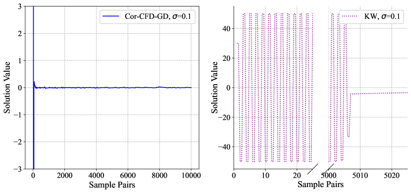
Figure 1: Solution value comparison between Cor-CFD-GD and SPSA algorithms across sample pairs for $\mu(x)=x^{4}$ with noise level $\sigma=0.1$.

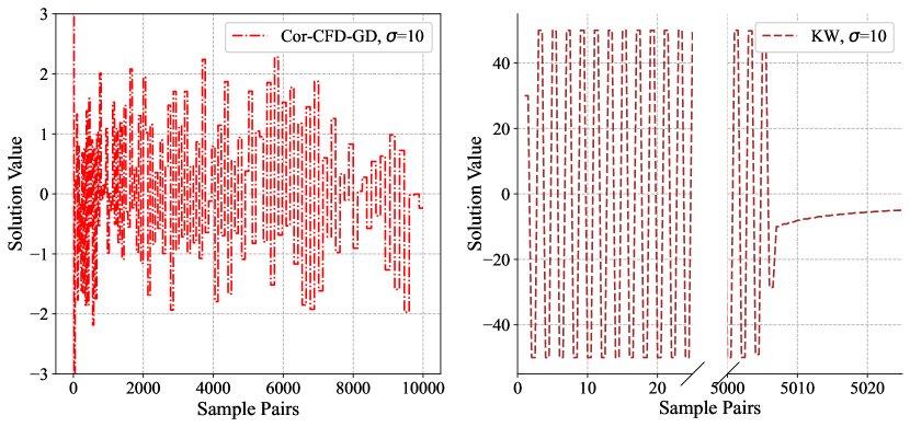
Figure 2: Solution value comparison between Cor-CFD-GD and SPSA algorithms across sample pairs for $\mu(x)=x^{4}$ with noise level $\sigma=10$.

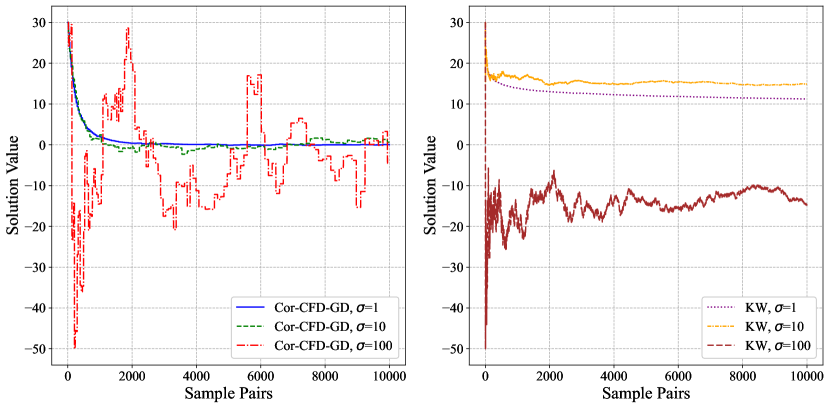
Figure 3: Solution value comparison between Cor-CFD-GD and SPSA algorithms across sample pairs for $\mu(x)=-100\cos(\pi x/100)$.

3.2 A Multi-Dimensional Example with SPSA

In this section, we consider the multi-dimension version of function 213 from Schittkowski (1987):

$$\mu(\textbf{x})=\sum_{i=1}^{d/2}\left[10(x_{2i}-x_{2i-1})^{2}+(1-x_{2i-1})^{2}\right]^{4},$$ (3.1)

where $d$ is a positive even integer representing the dimension of the input vector x.

The objective function reaches its global minimum of $0$ at $\textbf{x}^{*}=(1,\dots,1)$. The response surface is modeled as $Y(\textbf{x})=\mu(\textbf{x})+\epsilon(\textbf{x})$, where $\epsilon(\textbf{x})$ represents a zero-mean Gaussian noise with variance $\sigma^{2}$. Experiments are conducted with $d=64$ and varying noise levels $\sigma\in\{0.1,1,10\}$. Following the recommendation of Schittkowski (1987), we initialize the algorithm at $\textbf{x}_{0}=(3,1,\dots,3,1)$, where the function value is approximately $10^{8}$ at this starting point.

Fig. 4 shows the graph of function (3.1) with $d=2$, illustrating its optimization challenges. The graph exhibits a narrow, curved valley bordered by steep walls with large gradients. Near the optimum, the function becomes flat. Further from the optimum, the gradient magnitude increases, responding sensitively to small changes in x. This structure, characterized by steep outer regions and a relatively flat area near the minimum, poses substantial challenges for optimization.

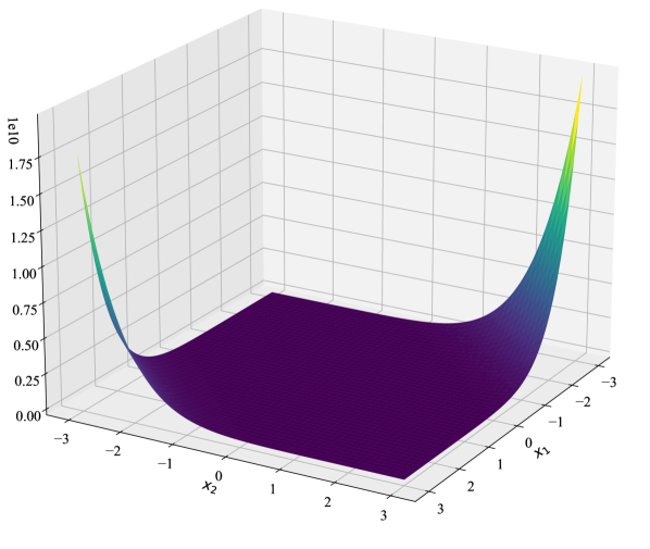
Figure 4: Image of function (3.1) at $d=2$.

As recommended in Spall (1998), the SPSA algorithm uses the parameters $a_{k}=a/(A+k+1)^{0.602}$ and $c_{k}=c/(k+1)^{0.101}$, where $A$ is 10% of the maximum number of sample pairs. To determine the optimal parameter configuration for SPSA under each experimental setting, we conduct a grid search over the parameter space. We evaluate combinations of the step size parameter $a\in\{10^{-1},10^{-2},10^{-3},10^{-4},10^{-5},10^{-6},10^{-7},10^{-8},10^{-9}\}$ and the perturbation parameter $c\in\{0.01,0.1,1,2,4\}$.

The optimal parameter settings are as follows: for budgets of 1,000 and 5,000, the parameter $a$ is consistently set to $10^{-9}$ across all variance levels, while $c$ remains constant at 2. For the budget of 10,000, $a$ increases slightly to $10^{-8}$, yet $c$ continues to hold steady at 2 regardless of variance. This parameter stability can be attributed to the relatively large function values during the initial stages of optimization, which effectively overshadow the impact of variance. The noise introduced by varying levels of variance does not significantly affect the optimization trajectory, allowing these parameter settings to perform optimally across different settings. Notably, increasing the step size $a$ causes the points to jump too far, preventing convergence, while decreasing $a$ results in very slow convergence.

We compare the RMSE(Solution Gap) and RMSE(Optimality Gap).

• RMSE (Solution Gap) is defined as the RMSE of the distance between the solution point and the optimal point $(1,1,\dots,1)$.

• RMSE (Optimality Gap) is defined as the RMSE of the distance between the obtained value and the optimal value $0$.

Table 3 presents results for function (3.1) with $d=64$, based on 200 replications for each configuration. Note that the actual sample pairs used in the table is $d$ times the values listed to account for the demands of this relatively high-dimensional setting. For the Cor-CFD-GD algorithm, we adhere to the original setup. For the SPSA algorithm, the results reflect performance under optimal parameters. Experimental results demonstrate that the Cor-CFD algorithm consistently outperforms the SPSA algorithm across all parameter settings tested, even when SPSA is optimized with its best parameters. For example, under setting with noise level $\sigma=1$ and sample pairs of 1000, the Cor-CFD-GD algorithm achieves RMSE (Solution Gap) of 77.24 and RMSE (Optimality Gap) of 7.203, while SPSA yields a higher RMSE (Solution Gap) of 117.30 and RMSE (Optimality Gap) of 232.58. The superior performance of the Cor-CFD algorithm over the SPSA algorithm can be attributed to fundamental differences in their gradient estimation strategies and step size adaptation mechanisms.

Table 3: Comparison of the Cor-CFD-GD algorithm and the KW algorithm for function (3.1).

		RMSE (Solution Gap)			RMSE (Optimality Gap)
$\sigma$	Method	1,000	5,000	10,000	1,000	5,000	10,000
0.1	Cor-CFD-GD	61.73	45.52	39.72	2.47	1.50	1.30
	SPSA	117.34	115.87	125.47	232.81	247.24	147.38
1	Cor-CFD-GD	77.24	57.92	50.22	7.20	4.66	4.26
	SPSA	117.30	116.11	125.28	232.58	247.96	125.36
10	Cor-CFD-GD	90.11	74.22	66.06	19.09	15.65	15.29
	SPSA	117.11	116.16	125.90	232.31	247.77	126.19

Since SPSA estimates the gradient using only two samples, its gradient estimation may lack accuracy. For function (3.1), the gradient is large near the starting points and becomes smaller near the optimal point. To avoid overshooting at the beginning, a small initial step size would be necessary. However, as the algorithm approaches the optimal region, this small step size restricts efficient convergence, significantly slowing down the optimization as it nears the optimal point.

Cor-CFD estimates gradients using multiple samples, enhancing both the accuracy and stability of its gradient approximations. This mitigates the risk of extreme directional jumps, improving robustness across different variance conditions. The Cor-CFD-GD algorithm employs an Armijo line search (2.4) to dynamically adjust the step size based on the gradient magnitude at each iteration. This approach allows the algorithm to adaptively select small step sizes when gradients are large (e.g., at the initial points), preventing overshooting and ensuring stable progression. As the gradient diminishes near the optimal point, Cor-CFD-GD can take larger steps, accelerating convergence in low-gradient regions. By combining batch-based gradient estimator with Armijo line search, Cor-CFD maintains stability in early iterations and avoids the slow convergence issues encountered by SPSA near the optimal point. Unlike SPSA, which is highly sensitive to initial step size, Cor-CFD’s adaptive step size strategy is more resilient, allowing it to perform well without the need for careful tuning of initial parameters.

Notably, the SPSA algorithm’s performance in the table remains unaffected by variance. In contrast, the performance of the Cor-CFD-GD algorithm declines as variance increases. This difference arises because SPSA’s slower convergence rate keeps it in regions with large function values relative to the noise for a longer period, where the influence of variance is minimal. Meanwhile, Cor-CFD-GD descends more quickly into regions where function values are comparatively small relative to the noise, which decreases the accuracy of its gradient estimates and, consequently, affects optimization performance.

Fig. 5 shows the changes in the solution gap for a single experiment with sample pairs of 1000, comparing the Cor-CFD-GD and SPSA algorithms across sample pairs. Similarly, Fig. 6 presents the changes in the optimality gap for Cor-CFD-GD and SPSA under the same budget, showing their respective performances over sample pairs. It is important to note that Cor-CFD-GD algorithm does not utilize all the sample pairs, as the remaining sample pairs are insufficient for Cor-CFD-GD to conduct a new gradient estimator. Initially, SPSA demonstrates better performance due to its higher iteration steps within the first 2500 sample pairs. However, once Cor-CFD-GD completes two iterations (approximately 40.36 sample pairs $\times$ 64, where $20\times 2$ sample pairs for Cor-CFD and 0.36 for line search), it begins to outperform SPSA, achieving a faster and more stable reduction in the optimality gap across all noise levels. Cor-CFD-GD’s superior long-term performance is attributed to its reliable gradient estimation method, enabling accurate descent direction and the use of larger step sizes for faster convergence. In contrast, SPSA uses only two samples to approximate the gradient, which results in a less precise descent direction and forces the algorithm to use smaller step sizes to maintain stability.

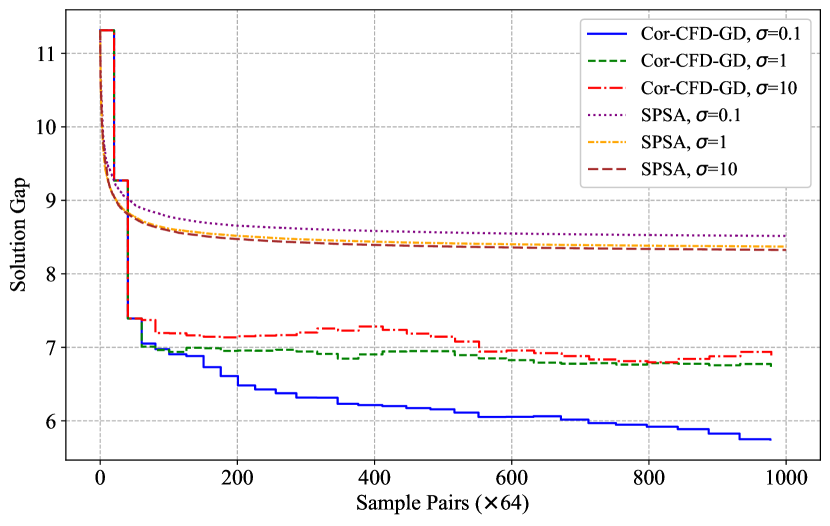
Figure 5: Solution gap comparison between Cor-CFD-GD and SPSA algorithms across sample pairs for function (3.1).

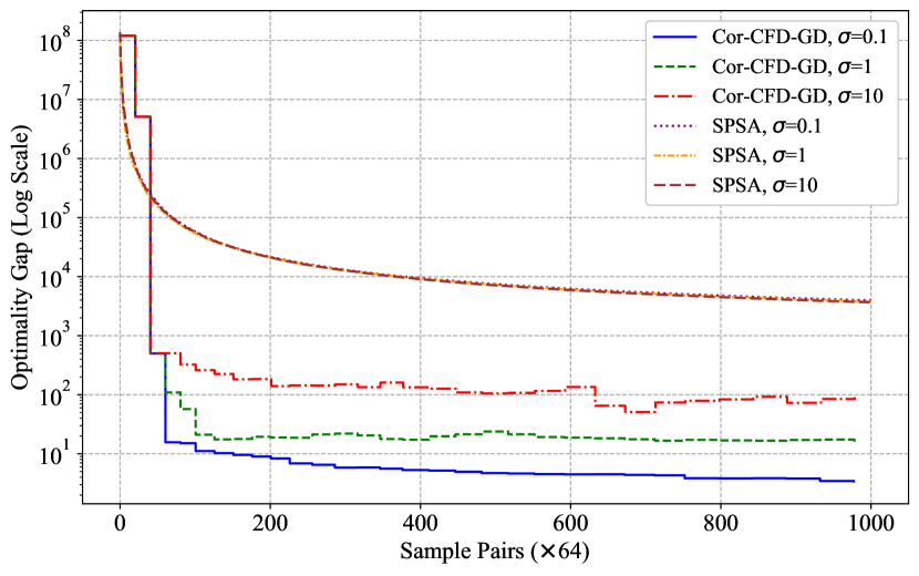
Figure 6: Optimality gap comparison between Cor-CFD-GD and SPSA algorithms across sample pairs for function (3.1).

4 Conclusions

In this paper, we have conducted experimental studies to investigate the trade-off between gradient estimation accuracy and iteration steps in DFO. Our results demonstrate that the Cor-CFD method, which prioritizes gradient estimation accuracy through careful sample utilization, outperforms traditional approaches such as KW and SPSA that favor frequent iterations with minimal samples. This superior performance is observed across both low-dimensional and high-dimensional settings, suggesting that the benefits of accurate gradient estimation outweigh the computational cost of additional samples per iteration.

Several promising directions for future research emerge from this work. First, developing adaptive sample allocation strategies that dynamically adjust the number of samples based on the optimization results could further enhance the efficiency of gradient estimation. Bollapragada et al. (2018) presents a promising solution for the L-BFGS algorithm. The second direction involves establishing the theoretical convergence properties of optimization algorithms based on Cor-CFD. The theory presented in Hu and Fu (2024) may offer some valuable guidance for this direction. Finally, exploring the application of these findings to specific domains, such as deep learning hyperparameter optimization and reinforcement learning, could yield practical benefits in these increasingly important fields.

References

- Berahas et al. (2019) Albert S Berahas, Richard H Byrd, and Jorge Nocedal. Derivative-free optimization of noisy functions via quasi-newton methods. SIAM Journal on Optimization, 29(2):965–993, 2019.
- Bollapragada et al. (2018) Raghu Bollapragada, Jorge Nocedal, Dheevatsa Mudigere, Hao-Jun Shi, and Ping Tak Peter Tang. A Progressive Batching L-BFGS Method for Machine Learning. In Proceedings of the 35th International Conference on Machine Learning, pages 620–629. PMLR, July 2018. URL https://proceedings.mlr.press/v80/bollapragada18a.html. ISSN: 2640-3498.
- Bollapragada et al. (2024) Raghu Bollapragada, Cem Karamanli, and Stefan M Wild. Derivative-free optimization via adaptive sampling strategies. arXiv preprint arXiv:2404.11893, 2024.
- Broadie et al. (2011) Mark Broadie, Deniz Cicek, and Assaf Zeevi. General bounds and finite-time improvement for the Kiefer-Wolfowitz stochastic approximation algorithm. Operations Research, 59(5):1211–1224, 2011.
- Chau and Fu (2015) Marie Chau and Michael C Fu. An overview of stochastic approximation. Handbook of Simulation Optimization, pages 149–178, 2015.
- Fox and Glynn (1989) Bennett L. Fox and Peter W. Glynn. Replication schemes for limiting expectations. Probability in the Engineering and Informational Sciences, 3(3):299–318, 1989.
- Fu (2015) Michael C Fu. Stochastic gradient estimation. Handbook of Simulation Optimization, pages 105–147, 2015.
- Golovin et al. (2017) Daniel Golovin, Benjamin Solnik, Subhodeep Moitra, Greg Kochanski, John Karro, and David Sculley. Google vizier: A service for black-box optimization. In Proceedings of the 23rd ACM SIGKDD International Conference on Knowledge Discovery and Data Mining, pages 1487–1495, 2017.
- Hu and Fu (2024) Jiaqiao Hu and Michael C Fu. On the convergence rate of stochastic approximation for gradient-based stochastic optimization. Operations Research, 2024.
- Kiefer and Wolfowitz (1952) Jack Kiefer and Jacob Wolfowitz. Stochastic estimation of the maximum of a regression function. The Annals of Mathematical Statistics, 23(3):462–466, 1952.
- Larson et al. (2019) Jeffrey Larson, Matt Menickelly, and Stefan M. Wild. Derivative-free optimization methods. Acta Numerica, 28:287–404, 2019.
- Li and Lam (2020) Haidong Li and Henry Lam. Optimally tuning finite-difference estimators. In 2020 Winter Simulation Conference (WSC), pages 457–468. IEEE, 2020.
- Liang et al. (2024) Guo Liang, Guangwu Liu, and Kun Zhang. A correlation-induced finite difference estimator. arXiv preprint arXiv:2405.05638, 2024.
- Robbins and Monro (1951) Herbert Robbins and Sutton Monro. A stochastic approximation method. The Annals of Mathematical Statistics, 22(3):400–407, 1951.
- Schittkowski (1987) Klaus Schittkowski. More Test Examples for Nonlinear Programming Codes, volume 282 of Lecture Notes in Economics and Mathematical Systems. Springer Berlin Heidelberg, Berlin, Heidelberg, 1987. ISBN 978-3-540-17182-9 978-3-642-61582-5. doi: 10.1007/978-3-642-61582-5. URL http://link.springer.com/10.1007/978-3-642-61582-5.
- Shi et al. (2023) Hao-Jun Michael Shi, Qiming Melody Xuan, Figen Oztoprak, and Jorge Nocedal. On the numerical performance of finite-difference-based methods for derivative-free optimization. Optimization Methods and Software, 38(2):289–311, 2023.
- Song et al. (2024) Xingyou Song, Qiuyi Zhang, Chansoo Lee, Emily Fertig, Tzu-Kuo Huang, Lior Belenki, Greg Kochanski, Setareh Ariafar, Srinivas Vasudevan, Sagi Perel, and Daniel Golovin. The vizier gaussian process bandit algorithm, 2024. URL https://arxiv.org/abs/2408.11527.
- Spall (1992) James C. Spall. Multivariate stochastic approximation using a simultaneous perturbation gradient approximation. IEEE Transactions on Automatic Control, 37(3):332–341, 1992.
- Spall (1998) James C. Spall. Implementation of the simultaneous perturbation algorithm for stochastic optimization. IEEE Transactions on Aerospace and Electronic Systems, 34(3):817–823, 1998. doi: 10.1109/7.705889.
- Xuan (2023) Melody Qiming Xuan. Methods for Derivative-Free Optimization with Applications in Machine Learning, volume PhD Thesis. Northwestern University, 2023.
- Zazanis and Suri (1993) Michael A. Zazanis and Rajan Suri. Convergence rates of finite-difference sensitivity estimates for stochastic systems. Operations Research, 41(4):694–703, 1993.