OE_^ OmOE_^ OmOE_^ Omm!OE_^ mmmmOE_^
Method of Moments for Estimation of Noisy Curves
Abstract.
In this paper, we study the problem of recovering a ground truth high dimensional piecewise linear curve from a high noise Gaussian point cloud with covariance centered around the curve. We establish that the sample complexity of recovering from data scales with order at least . We then show that recovery of a piecewise linear curve from the third moment is locally well-posed, and hence samples is also sufficient for recovery. We propose methods to recover a curve from data based on a fitting to the third moment tensor with a careful initialization strategy and conduct some numerical experiments verifying the ability of our methods to recover curves. All code for our numerical experiments is publicly available on GitHub.
1. Introduction
1.1. Motivation and Related Work
Manifold learning is a widely-studied problem in statistics in which a low dimensional manifold is fit to high dimensional data in an effort to understand the geometry of the data and circumvent the curse of dimensionality. A vast amount of literature has been dedicated to the noise-free case, where the data lie exactly on some lower dimensional manifold; see, for instance, [16] for a review of more classical methods, or [8], [18] for more recent results. Work has also been done in the case of low noise, such as in [28], [6], [27], [26], and [14]. Less work has been done for the more difficult high noise case, in which each data point is completely dominated by noise. In [7], the authors establish an algorithm for recovering manifolds with particular smoothness properties corrupted by Gaussian noise with covariance for arbitrary , but their algorithm requires a number of samples exponential in .
Another field in which recovering a signal from high noise has been studied is in orbit recovery problems. In these problems, an underlying signal is corrupted by some group action and a large amount of additive noise, and the goal is to recover the original signal. Perhaps the most famous such problem is the reconstruction of the 3D structure of macromolecules from cryo-electron microscopy (cryo-EM) images. In cryo-EM, a large number of extremely noisy images are taken of a molecule in various 3D orientations. We can think of these images as projections of an unknown rigid rotation of the Coulomb potential along an axis to a two-dimensional image that is then corrupted by a large amount of Gaussian noise. The task of recovering thus involves both denoising the Gaussian noise and undoing the rotation. See [23] for a comprehensive review of computational aspects of Cryo-EM. A simpler orbit recovery problem that has been well-studied is the multireference alignment (MRA) problem. In the MRA model, the ground truth is a one-dimensional signal and the measurements consist of a random cyclic permutation of corrupted with additive Gaussian noise. The sample complexity of MRA is established in [21], where the authors prove that for large , any algorithm hoping to recover must require samples.
We are interested in recovering one-dimensional manifolds (i.e., curves) in high dimensions in the presence of large Gaussian noise. For a particular class of curves, we will establish the sample complexity of the problem to be and provide a recovery algorithm that meets that lower bound. The setting of one-dimensional manifolds corresponds to temporal data, and we can think of noisy curves as noisy measurements of some system evolving in time; recovering the underlying curve thus corresponds to recovering the underlying dynamics. In the one-dimensional setting, a great deal of work has been done in the seriation problem, where noisy observations of time-dependent data are labeled with ordered timestamps. For instance, in cryo-EM, one might have noisy observations of a biological macromolecule undergoing some conformational change over time; in this context, the seriation problem involves estimating the temporal order of these conformers (see for instance [19], [15]). In archaeology, seriation techniques are used to date archeological finds [10]. Various spectral methods have been developed for the seriation problem ([2], [9], [22]), but often require strong structural assumptions on the data. More recently, the authors in [13] use the Fiedler vector of the graph Laplacian of the data to approach the seriation problem in a more general case. Note that our problem is not to only recover the time ordering of noisy points coming from a curve, but to recover the underlying curve itself. If the distribution of the noise is known, then the time ordering of noisy points can be computed from the underlying curve simply by associating each noisy data point with a point in the underlying curve that maximizes the likelihood.
1.2. Problem Formulation: Noisy Curve Recovery
Consider a parametric, non self-intersecting ground truth piecewise linear (PWL) curve in , . We assume that the curve consists of a finite number of segments. In order to fix a scale, we assume that for all . The noisy curve model consists of independent observations
| (1.1) |
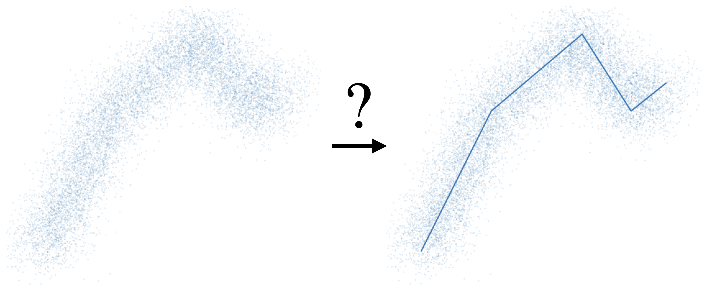
Here is drawn uniformly randomly and denotes isotropic Gaussian noise independent of ; we assume is known. We can imagine this as a Gaussian “fattening” of the curve . Let denote the random variable given by , and let denote the case where . We formulate the noisy curve recovery problem as the estimation of from observations , as depicted in Figure 1. Note that we can think of this model as a continuous Gaussian mixture model, where the mixture centers are drawn continuously from .
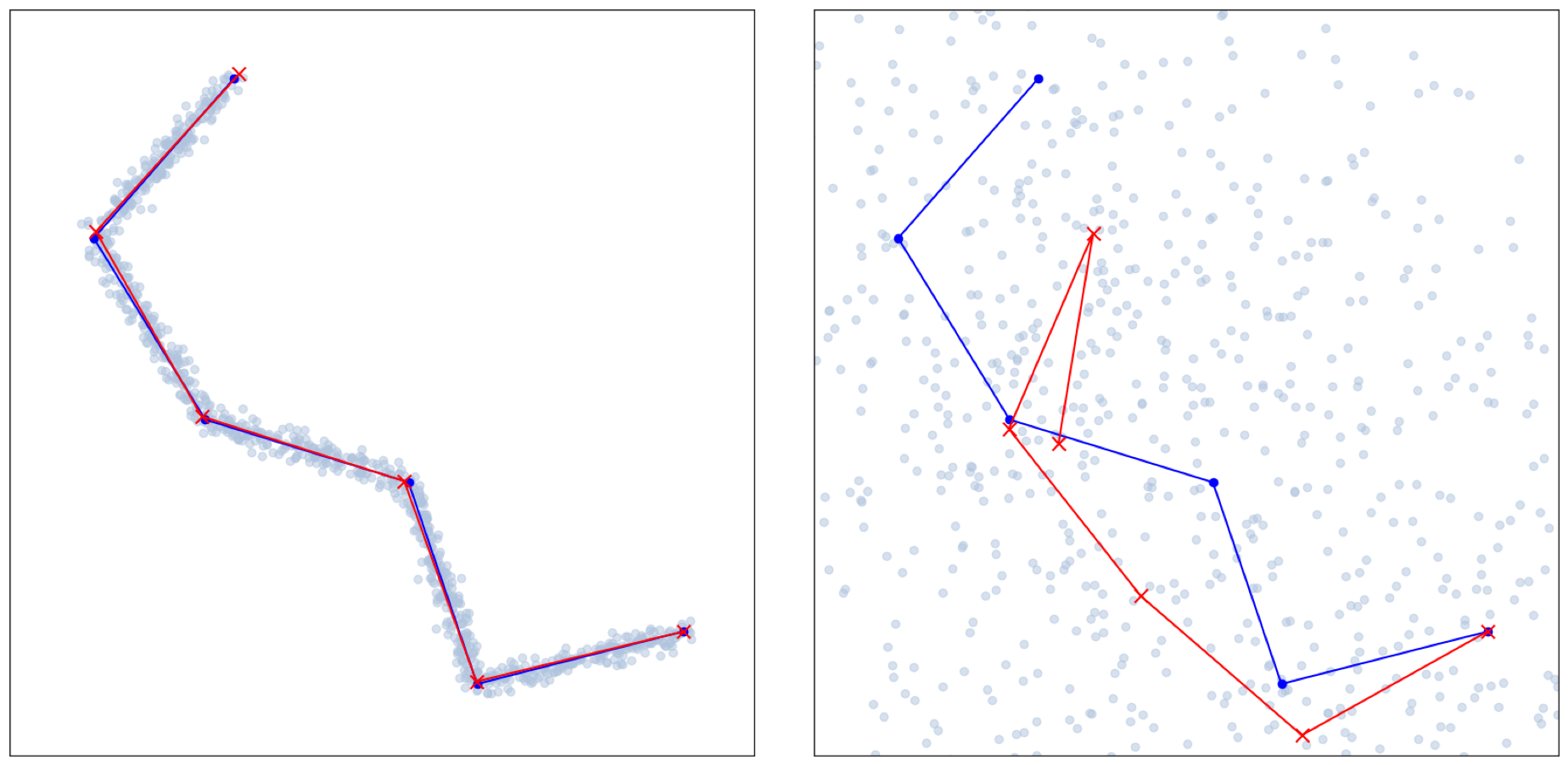
In the low noise regime, the salient features of the underlying curve are still visible in the presence of noise, and the curve can be estimated by “tracing through” the point cloud coming from (1.1). We provide a more detailed account of an algorithm in Appendix A, but essentially, much like the expectation-maximization step in estimating finite Gaussian mixture models, we can assume that nearby points in the cloud come from nearby points on the underlying curve. We can thus use the local largest principal component of subsets of the point cloud to approximate the tangent space of the curve near that point. However, in the case where noise is large, we can no longer reliably assign points in the point cloud to a nearby point on the underlying curve. This is illustrated in Figure 2, where we demonstrate the results of tracing through a point cloud coming from a PWL curve in both the low and high noise case. We are henceforth interested in studying the high noise case.
In this paper, we will first prove a result on the sample complexity of the high noise curve recovery problem, that is, the number of samples needed to recover the ground truth underlying curve from data up to some error. In particular, we will show that for sufficiently high noise, the number of samples from (1.1) needed to recover a curve scales with order . The proof relies on studying the moments of the distribution , particularly the third moment. Our approach is based largely on the approach in the proof of the sample complexity of the MRA problem in [21]; the proof hinges on showing that the first two moments alone do not uniquely determine a curve in a neighborhood. We then prove that the problem of recovering the underlying curve from the third moment of the data is in fact locally well-posed, and provide an algorithm to obtain an initial rough estimate of the curve based on a decomposition of the third moment tensor of the curve. The idea of the algorithm is to use the tensor power method to approximate the subspaces in which vertices of the curve lie, then use this as an initialization to a gradient descent scheme to fit a curve defined by the vertices to the third moment.
1.3. Paper Outline
The paper is organized as follows. In §2, we introduce notation for piecewise linear curves and compute their moments. In §3, we state and outline the proof of the sample complexity result. In §4, we show that locally, the third moment uniquely determines piecewise linear curves in high dimensions. In §5, we use this local well-posedness to devise an algorithm that recovers piecewise linear curves. We show results from numerical experiments demonstrating the performance of our algorithm in §6.
2. Piecewise Linear Curves and their Moments
We restrict our analysis to piecewise linear (PWL) curves in order to have a simple explicit representation of a curve. We also require that our curves have domain , are open, and have constant speed, i.e., is constant.
Let be points in time and let be the vertices of a PWL curve. Throughout this paper, we use to denote the ambient dimension of the curve and to denote the number of segments. We assume in general that our dimension is high enough that . We also assume that for all . In particular , so our curve is open.
We have the following explicit expression for :
| (2.1) |
Since we require to have constant speed, we must have
| (2.2) |
where is the total length of the curve. The benefit of requiring constant speed is that our curves are completely characterized by the vertices . In a slight abuse of notation, we thus identify a PWL curve with the -shaped matrix of its row-stacked vertices:
| (2.3) |
We assume that the are in generic position, so that the vectors are linearly independent.
Our approach to proving lower bounds on the sample complexity of noisy curve recovery is based on studying the moments of a curve, defined by
| (2.4) |
Here, denotes the -fold tensor power of a vector. For instance, for , is the -shaped tensor whose entry is given by . The use of moment tensors for inverse problems has been studied in many other contexts, such as finite Gaussian mixture models in [20].
We now derive expressions for the first three moments of in terms of the vertices .
Proposition 2.1 (Moments of Piecewise Linear Curves).
Let be the constant speed PWL curve with domain with vertices . Let be the length of . Then the first three moments of are given by the formulas
| (2.5) | ||||
Proof.
Consider the change of variables
| (2.6) |
For any , we can apply this change of variables and (2.2) to get an expression for in terms of the vertices :
| (2.7) | ||||
The desired result can be obtained by expanding the tensor power in the integral for and direct computation of the integral. ∎
Recall our assumption that and observe that a PWL curve with segments naturally lives in an -dimensional subspace of spanned by the vectors . We can in fact compute an orthonormal basis for this subspace by taking the top eigenvectors of the second moment ; indeed, the second moment is a rank- matrix for generic . Therefore we will often assume , since if , we can project the coordinates of down to . Nonetheless, for semantic clarity, we will often use when referring to the number of segments and when talking about the dimension.
Later on in the paper, we will show two important results involving moment matching. We will show that matching a PWL curve to a third moment is locally well-posed, while matching a PWL curve to the first two moments and is locally ill-posed. A careful analysis of the moments is difficult owing to the terms (note that also depends on ). To aid in our analysis and make things easier to compute, we introduce the following relaxed curve moments that replace the terms with new variables. We will show that it is sufficient to consider moment matching in this relaxed setting.
Definition 2.2 (Relaxed Curve Moments).
Let and . Then we define the relaxed moments of to be
| (2.8) | ||||
We can rewrite these in a more vectorized way that makes our analysis more straightforward.
| (2.9) | ||||
Here, is an -shaped matrix constant and is a symmetric -shaped matrix that is a linear function of . The six-way tensor has shape and has entry given by . The three-way tensor is a linear function of and is symmetric with shape . The operation denotes the natural tensor contraction between tensors of shape and :
| (2.10) |
The exact forms of , , and are given in Appendix D. Note that in the case where is the vector of proportional segment lengths of , i.e., for all , the relaxed moments are precisely equal to the actual moments.
We now present expressions for the Jacobians of the error between a predicted relaxed third moment and a ground truth third moment. The proof is by standard matrix calculus techniques, which we omit.
Lemma 2.3 (Jacobians of Relaxed Moments).
Let be the matrix representation of a PWL curve and ; note that we do not require to be equal to the proportional segment lengths of . Let be some third moment tensor. Define the third moment loss
| (2.11) |
where is the squared Frobenius norm on tensors, i.e., the sum of the squared entries. Let and . Let be as in (D.3) and be as in (2.10). Then the derivatives of the third moment loss with respect to and applied to and respectively are given by
| (2.12) | ||||
3. The Sample Complexity Lower Bound
To talk about the sample complexity of recovering PWL curves, we need a measure of the distance between two curves. We choose the following natural distance.
Notation 3.1.
Let and be two non-closed parametric curves on . Then we define the distance between the two curves to be the average squared Euclidean distance between the curves:
| (3.1) |
We assume that is parameterized so that ; i.e., is oriented in the direction that minimizes the distance.
We first prove that curve recovery from the first and second moment alone is not locally well-posed. In other words, we can find two curves that are arbitrarily close together with exactly the same first and second moment. As discussed in §2, we assume that the number of segments is equal to the ambient dimension .
Proposition 3.2.
Let be a PWL constant speed curve with segments. For almost all such , for sufficiently small , there exists a PWL curve with and such that , where the norm here is on the matrix representation of the curves.
The detailed proof is provided in Appendix B; the idea is that matching the first and second moment of a curve can be expressed as an underdetermined system of polynomials whose solutions form a manifold of positive dimension.
Since and being close as matrices implies that and are close as curves, we have the following immediate corollary of Proposition 3.2.
Corollary 3.3.
As in Proposition 3.2, let be a PWL constant speed curve with segments. For almost all such , for sufficiently small , there exists a PWL curve with and such that for all .
The application of Corollary 3.3 is to show that the hypotheses of the following result are not vacuous for . The proof is rather technical and left to Appendix C.
Proposition 3.4.
Let , be mean zero parametric curves such that and for all . Suppose for all . Then for , we have the following bound on the divergence between and :
| (3.2) |
where is a constant that depends on only.
This result allows us to bound the divergence between two noisy curve distributions by if the moments of the underlying curves match up to (but not including) order . This is the primary ingredient in the proof of the following main sample complexity result. Note that we use to denote inequality up to a universal constant.
Theorem 3.5.
Let be a curve as in be as in Proposition 3.4. Given any sufficiently small, there exists another curve satisfying the hypotheses of Proposition 3.4 such that , where is indistinguishable from in the following sense. Consider samples and the task of deciding if came from or . Assume a uniform prior on whether the ground truth curve is or . Then if , the probability of making an error is bounded below by .
Proof.
Given , construct such that the first two moments match and as in Proposition 3.2. Then by Theorem 3.4, we have the bound . By Lemma E.3, Lemma E.4, and Lemma E.5,
| (3.3) |
Therefore, for , we have
| (3.4) |
Now let be any measurable function of the data . Let denote the set of all such that . Then
| (3.5) | ||||
Let denote the event that the ground truth curve is and denote the event that the ground truth curve is . By our uniform prior assumption, we have . Then the probability of the hypothesis test making an error is
| (3.6) | ||||
∎
This result reveals a fundamental limitation of the curve recovery problem in the high noise regime; regardless of the method used, it is impossible to discern with high probability which of two -separated curves the data come from without at least samples.
4. Local Well-Posedness of Third Moment-Based Recovery of Piecewise Linear Curves
Theorem 3.5 gives us a lower bound of on the sample complexity of recovering a curve from data. We now show that for PWL curves with constant speed, this lower bound is asymptotically tight by showing that is indeed enough samples for recovery. We accomplish this by showing that the third moment of a noise-free PWL curve uniquely determines a PWL curve in a neighborhood. This is contrast to the result of Proposition 3.2, which says that determining a curve from the first two moments alone is locally ill-posed. As before, in this section we assume .
Our ultimate goal in this section is to show the following.
Theorem 4.1.
Let be a ground truth PWL curve with proportional segment lengths , where . Let be the ground truth third moment. Let be the third moment squared Frobenius loss as defined in (2.11) Then for almost all , if is sufficiently close to and is sufficiently close to , we have
| (4.1) | ||||
| (4.2) |
Local well-posedness of recovery from is an immediate corollary of this.
Corollary 4.2.
Let , , and as in Theorem 4.1. Then for almost all , there exists a neighborhood of such that is the only PWL curve in with third moment .
Proof.
The result of Theorem 4.1 implies that is an isolated minimum of . ∎
To prove Theorem 4.1, we will first need the following weaker result.
Lemma 4.3.
Let be a ground truth PWL curve with proportional segment lengths , where . Let be the ground truth third moment. Then for almost all , for sufficiently close to and sufficiently close to , we have
| (4.3) | ||||
| (4.4) |
Equation (4.3) differs from (4.1) in that we have replaced the in with , and similarly for (4.4) and (4.2). In other words, (4.3) says that recovery of from and is locally well-posed, while (4.4) says that recovery of from and is locally well-posed. On the other hand, the stronger statements (4.1) and (4.2) say that recovery of and from is locally well-posed. We prove (4.3) in §4.1, (4.4) in §4.2, and (4.1) and (4.2) in §4.3.
4.1. Recovery of from
Let be sufficiently small and be some other curve in a neighborhood of . Then we wish to show that for sufficiently close to , we have
Using (2.12), the left hand side of (4.3) becomes
| (4.5) |
We perform a Taylor expansion, replacing with , expanding the nonlinear terms and only keeping terms with one . Then (4.5) has first order approximation given by
| (4.6) |
Let be the term inside the norm:
| (4.7) |
This is a linear operator from . Therefore, to show (4.3), it suffices to show that the kernel of is trivial.
Let denote the symmetrization operator on three-way tensors, i.e.,
| (4.8) |
Note that is linear. Then by the definition of the operation and the symmetry of , we can rewrite (4.7) as
| (4.9) |
Let denote the term inside the :
| (4.10) |
To show that has trivial kernel, it suffices to show that has trivial kernel and (b) . We prove (a) in Lemma 4.4 and (b) in Lemma 4.6.
Lemma 4.4.
Let . Let and assume that are in generic position so that any collection of of the ’s is linearly independent. Let be the linear operator given in (4.10). Then has trivial kernel.
Proof.
Note that is a linear operator from . If we think of this as a matrix operating on the flattened spaces, then with our assumption of , the matrix representation of is a tall and thin matrix. To show that has trivial kernel, it suffices to show that the “columns” of are linearly independent.
Let be the standard basis matrix in with all zeros except a in the entry; note that ranges from to while ranges from to , i.e. we zero-index the rows but one-index the columns. Then the “column” of is given by . Let denote the th row of , which is equal to (the th standard basis vector in ) if and zero otherwise. Then
In the last line, we are notating a -shaped tensor as a size vector consisting of size matrices, where the matrix is in the th slot of the vector and is given by
| (4.11) |
From the position of the nonzero entries, it is clear that are linearly independent for fixed and varying . It remains to show that there is also linear independence for fixed and varying ; in other words, we need to show that is a linearly independent collection of matrices; we verify this in Lemma E.6. ∎
Before we show , we first need the following result, which we have adapted from Lemma 5.6 in [11].
Lemma 4.5.
Let be a matrix whose entries are analytic functions of a variable for some connected open domain . Let be the rank of for some particular . Then for almost all .
Proof.
Note that if and only if the determinant of every -shaped minor of vanishes. Since the rank of is , there exists some -shaped minor such that . Note that is an analytic function of , and the witness shows that is not identically zero. An analytic function that is not identically zero has a measure zero vanishing set (see [17]). Therefore, has a vanishing set of measure zero, and hence is on a measure zero set. ∎
The utility of this lemma is that if a matrix has entries that are analytic and we find a single witness such that is full rank, then we know is full rank for almost every . We use this lemma in the proof of the following result.
Lemma 4.6.
Let and . Then for almost all , the image of and the kernel of are linear subspaces that intersect only at .
Proof.
In the proof of Lemma 4.4, we showed that forms a basis for . Since the action of depends on , in this proof we will use the notation to denote the operator induced by a particular choice of . For coefficients , we wish to show that if
| (4.12) |
then all the coefficients must be zero. By linearity of the operator, it suffices to show that
| (4.13) |
forms a linearly independent set of -shaped tensors.
Let denote the -shaped matrix of column-stacked flattenings of the tensors in (4.13). Then we wish to show that this matrix has full column rank for almost all . The entries of are either zeros or linear combinations of the entries of as defined in (4.11). Recall that the values are a function of in the following way:
| (4.14) |
On the connected open domain , this is an analytic function of the entries of . Since the entries of terms of the form and are also analytic, it follows from the form of that the entries of are analytic functions of the entries of . By Lemma 4.5, it suffices then to find a single witness for each dimension where has full rank.
For , we define the following witness (for notational clarity, we show the case here, with for greater being defined in the obvious way):
| (4.15) |
We choose this particular because it induces matrices that are sparse and have a particular recursive structure, and the proportional segment lengths of are all . Define
| (4.16) | ||||
To show that is a witness for a full rank , it suffices to show that for all , is a linearly independent collection of tensors. We proceed by induction. The base case can be verified by straightforward computation. We verify this numerically by computing the singular value decomposition of the matrix and observing that the smallest singular value is positive; the smallest singular value is approximately .
Now suppose is a linearly independent collection; we wish to show that also is a linearly independent collection. Note that is an -shaped tensor. Let denote the -shaped “minor” of given by the subtensor of (here we are -indexing). By straightforward explicit computation of the entries of and , it can be shown that the minors of have the following properties:
-
(a)
For , : .
-
(b)
For : .
-
(c)
For : .
-
(d)
For : .
-
(e)
For : .
Now given coefficients , suppose
| (4.17) |
To complete the inductive step, it suffices to show that all coefficients must be zero. Observe that the subtensor of the linear combination above must also be zero, and hence using the properties above we have
This is a linear combination of the terms ; by the inductive hypothesis, this is a set of linearly independent tensors. In the last line above, we see that all in the first sum must be zero and all in the second sum must be zero. Therefore all in the third sum of the last line must be zero, and hence all in the third sum must be zero as well. We can thus conclude that in (4.17), all must be zero. Therefore, most of the terms in (4.17) vanish, and we are left with
| (4.18) |
Now consider the slice of the above tensor equation, which must equal the zero matrix. For , the slices of and are as follows, with the slices for greater values of being the obvious extension of the below (with the nonzero values being the same and more zero padding).
| (4.19) |
One can show that for all dimensions , these matrices are all linearly independent, and hence the remaining coefficients in (4.18) must also all be zero. Therefore, all coefficients in (4.17) must be zero, and hence is a linearly independent collection, as desired. ∎
This completes the proof of (4.3) holding for almost all .
4.2. Recovery of from
Now we wish to show that for sufficiently close to , we have (4.4), which we repeat here for convenience:
We can actually show a stronger statement, that the above is true for all . Using (2.12) and the fact that is linear in , we have
Unpacking the definition of and the operator, the term inside the norm on the last line is equal to
| (4.20) |
It suffices to show that this is equal to zero if and only if for all . In other words, we need to show that
| (4.21) |
is a collection of linearly independent three-way tensors for in generic position. We omit the proof of this because it uses techniques very similar to that of the proof of Lemma E.6. This completes the proof of (4.4) and hence the proof of Lemma 4.3.
4.3. Recovery of and from
We first prove (4.1), which we repeat here; we wish to show that for sufficiently close to and sufficiently close to , we have
For notational convenience, let us introduce the shorthand
| (4.22) |
We wish to write the expression in (4.1) in terms of (4.3) plus an error term. Using (2.12) and the fact to compute the difference and regrouping terms, we get
| (4.23) | ||||
The first term on the right hand side above is precisely the term in (4.3), which we showed was strictly negative for close to in §4.1. By linearity of , the remaining three terms on the right hand side go to zero as , and hence can be made arbitrarily small for close to by continuity. Hence, for sufficiently close to , the entire right hand side is strictly negative, and we have (4.1); we denote the neighborhood around for which (4.1) holds with .
Now we prove (4.2), which we also repeat; we wish to show that for sufficiently close to and sufficiently close to , we have
Similarly to before, now we wish to write the expression in (4.2) in terms of (4.3) plus an error term. Again using (2.12) and regrouping terms, we get
| (4.24) | ||||
Once again, the first term on the right hand side is precisely the term in (4.4), which we showed was strictly negative for all in §4.2. By continuity of the function , the remaining six terms on the right hand side go to zero as , and hence can be made arbitrarily small for close to . Therefore there exists a neighborhood of where (4.2) holds.
5. A Third Moment-Based Recovery Algorithm
Now we turn our attention to devising an algorithm to recover PWL curves from data. We assume that we have noisy observations coming from (1.1) of a ground truth PWL curve in with segments. We assume that . We also assume that is mean zero and that the points are in generic position.
Theorem 4.1 suggests that a reasonable approach is to first obtain a rough estimate with proportional segment lengths in a neighborhood near the ground truth , then perform gradient descent in and on the relaxed third moment loss (2.11), using and as initializations. We propose an algorithm that does exactly this, where the initial rough estimate is obtained via the tensor power method. Note however that applying Theorem 4.1 requires knowledge of the noise-free third moment of a curve. We therefore need a method of estimating noise-free moments from data.
In §5.1, we derive unbiased estimators of the noise-free curve moments from data. In §5.2, §5.3, and §5.4, we describe our recovery algorithm; in §5.2, we discuss how to use the tensor power method to estimate an unordered list of subspaces that the vertices of live on; in §5.3, we discuss how to reorder these subspaces; in §5.4, we use these reordered subspaces to obtain initial estimates and as initializations for a gradient descent scheme.
5.1. Unbiased Estimators of Noise-Free Moments
Our task is to recover a ground truth curve from observations , , where and . We want a way of recovering the noise-free moments of the curve from data. With , we define the th empirical moment of the data to be
| (5.1) |
First we recall the first three uncentered moments of a multivariate Gaussian.
Lemma 5.1.
(adapted from [12]) Let be a multivariate normal. Then the first through third uncentered moments of are given by
| (5.2) | ||||
Here, we use to denote the three-way tensor whose entry is .
From Lemma 5.1, we can compute unbiased estimators for the noise-free moments.
Lemma 5.2.
Let be such that and let , where and . Then
-
(1)
is an unbiased estimator of ;
-
(2)
is an unbiased estimator of ;
-
(3)
is an unbiased estimator of .
Proof.
For the first moment:
| (5.3) | ||||
For the second moment, eliminating cross terms by independence and the fact that and are mean zero, we can compute
| (5.4) | ||||
For the third moment, eliminating terms with the same idea, we have
| (5.5) | ||||
∎
Lemma 5.2 and the law of large numbers imply that the empirical moments , , and can estimate the noise-free moments , , and arbitrarily well (in probability) with a sufficient number of points as long as the noise level is known. Therefore, we will design our algorithm for curve recovery from data assuming that we have estimates , , and from (5.1) that are arbitrarily close to the ground truth moments , , and of .
Note that for coming from a noisy curve with noise level , the entries of have variance on the order of , so by Chebyshev’s inequality, the number of points needed to estimate the first three moments is order . A third moment-based recovery algorithm thus shows that the sample complexity lower bound in Theorem 3.5 is asymptotically tight.
5.2. Recovering the Subspaces of with the Tensor Power Method
Let be a three-way tensor of the form
| (5.6) |
where the vectors are orthonormal and the scalars are all positive; such tensors are called orthogonally decomposable. The tensor power method (TPM) is a robust iterative algorithm that is able to recover , up to some permutation of the indices. For that are unit length and independent (but not necessarily orthonormal), a whitening preprocessing step can be applied to reduce the problem to orthogonally decomposable case through an invertible linear transformation. A thorough introduction to the tensor power method as well as robustness guarantees can be found in [1]; we will take the TPM for granted in this paper. We summarize the TPM with whitening as presented in [1] in Algorithm 1. Note that for a -shaped tensor and matrix , we use to denote the tensor contraction of the three indices of with the first index of , i.e.,
| (5.7) |
We use the TPM in our algorithm in the following way. Recall from (2.5) that the third moment tensor of a ground truth PWL curve is given by
| (5.8) |
If we heuristically assume we can throw away the cross terms from , then this becomes a tensor of the form
| (5.9) |
We conjecture that the TPM with whitening applied to will recover unit vectors , such that after reordering, approximately spans the one-dimensional subspace that lives in, that is, is close to in cosine similarity.①①①The cosine similarity of two vectors and is . Throughout this subsection, we will use to refer to the unsorted unit vectors and to refer to the sorted unit vectors.
Note that (5.6) is invariant to a reordering of the ’s and ’s, so the fact that the TPM recovers up to permutation is not important to the tensor decomposition problem. However, to recover the vertices of a curve, we do in fact need to recover the ordering of the ’s. Therefore, we need some way to reorder the putative subspaces returned by the TPM.
5.3. Reordering the Predicted Subspaces
The tensor power moment returns unit vectors that are ostensibly close in alignment to the ground truth points ; we need to reorder them so that is close to , where we use the term “close” here (and in the rest of this subsection) in the sense of cosine similarity. The seriation problem of ordering time dependent data is well-studied and there are many existing approaches (see, for instance, [13], [9]), but here we outline a heuristic approach that empirically performs well for our purposes.
A reasonable prior is that our curve is sufficiently smooth such that if , then the two points closest to are and . This is the inspiration behind Algorithm 2, where we order the subspaces (given an initial choice) by iteratively choosing the closest subspace from that has not been sorted yet.
Algorithm 2 can output up to different orderings depending on the choice of initial index . To see which ordering to choose, consider the simple case illustrated in Figure 3. Here we assume that we have five unit vectors along some arc. Then the five possible orderings output by Algorithm 2, depending on the choice of initial index, are
-
(1)
-
(2)
-
(3)
-
(4)
-
(5)
.

Notice that the two correct sortings are (1) and (5), and that these two sortings are palindromes of another. A reasonable heuristic then is to assume that does not deviate too much from this ideal situation and do not deviate too much from the true subspaces, build up the chains starting from each of the predicted subspaces, and choose the chain that has a palindrome.
Of course, in general we are not guaranteed that a palindrome pair will exist among the sortings generated by Algorithm 2, so we instead need a way to measure how “palindromic” a particular sorting is given a list of sortings.
Definition 5.3.
Let be a set of permutations of elements, where we identify permutations with ordered tuples of length with exactly one of in each entry. Let be the reversed tuple of . Given , we define the palindrome similarity between them as the number of entries in which and agree. For example, . The palindromicity of a permutation is defined as the maximum palindrome similarity between and every other permutation in :
| (5.10) |
Note that if the palindromicity of a permutation in a list is equal to , that means the palindrome of the permutation exists in the list. From our list of orderings generated by the chain-building algorithm, we then choose the one with the highest palindromicity, breaking ties arbitrarily. In the ideal case, there should be exactly one pair of orderings with palindromicity equal to .
5.4. Final Optimization Steps
From the output of Algorithm 1 sorted by Algorithm 2, we now have a row-stacked matrix of unit vectors that approximately span the subspaces in which lie. Since are unit length, we now wish to find scalars such that the curve with vertices has moments close to the estimated moments . Observe that is the matrix whose th row is given by . Then we choose to minimize the loss of the first three moments of :
| (5.11) |
If the are close in alignment to , then should be close to the ground truth . If this is close enough, then it will be within the neighborhood of where the third moment minimizer is unique (the existence of such a neighborhood is precisely the statement of Corollary 4.2). We call this first step the initial estimate phase.
With determined, we now use as an initialization for gradient descent on as defined in (2.11). In practice, as mentioned in §2, since naturally lives in an -dimensional subspace of , we first project down to the subspace spanned by the top eigenvectors of ; let be the -shaped matrix whose columns are these eigenvectors. Note that if we replace the estimate with the exact second moment of , then has exactly nonzero eigenvectors. Then the projection of onto can be estimated by (the estimation is exact when is computed from rather than ).
Since we wish to match the third moment in the subspace , we need to estimate the third moment of the projected curve. The exact third moment of the projected curve is given by (see (5.7)), and hence we can estimate the projected third moment from data by . We then use and its corresponding proportional segment lengths as an initial point for minimizing via alternating gradient descent, then deproject the result back to to get our final prediction . We call this second step consisting of projection, alternating descent, and deprojection the finetuning phase.
To summarize, our recovery algorithm is in two phases. The first initial estimate phase uses the TPM on the third moment tensor to approximately recover the unordered subspaces in which the points approximately lie; these points are then sorted using the chain-building algorithm, and the sorting with the best palindromicity is chosen. We then find the best along these subspaces that minimize the loss of the first three moments. In the second finetuning phase, we use these as an initial guess for minimizing the loss of the relaxed third moment in the -dimensional subspace where naturally lies. The full algorithm is presented as Algorithm 3.
6. Numerical Results
Here we present some numerical results on using Algorithm 3 to recover curves. Our implementation is primarily built with the the libraries JAX and JAXopt ([5], [4]) and available on GitHub②②②https://github.com/PhillipLo/curve-recovery-public.
To generate our data, we first prescribe segment lengths uniformly randomly from the interval . Then we sample a random curve in with segments by choosing the origin as the initial point, then iteratively adding points by choosing a random vector on the sphere with radius and adding it to the most recently generated point on the curve. We then subtract away the first moment of the curve to ensure that our curve is mean zero. We do not normalize the segment lengths to fit the curve into the unit ball (as in the hypotheses for Proposition 3.4) for numerical stability reasons.
Recall Algorithm 3 relies on having access to the noise-free moments of the ground truth curve . For high noise, a very large number (order ) of data points from a noisy cloud are required to closely estimate the first three moments of the noise-free underlying curve. In high dimensions, this becomes enormously computationally expensive. Therefore, we show results from two different experiments: one where we apply Algorithm 3 directly on ground truth noise-free moments that we obtain from (i.e., we set ), and another experiment that uses empirical moments computed from a point cloud generated from (i.e. we estimate from data). Due to the large number of points needed to accurately estimate the third moment tensor, we compute the moments in an online manner so that we never have to store an entire point cloud in memory.
Algorithm 3 involves an initial phase that estimates a curve close to the ground truth before a second phase that directly minimizes the relaxed third moment loss. We propose two similar baseline algorithms to show that our initial rough estimation phase is essential: we simply directly minimize either the squared Frobenius loss of the third moment or the sum of the losses of the first, second and third moments from multiple random initializations, as detailed in Algorithm 4. We perform the optimization in an estimation of the natural -dimensional subspace where the curve lies, so we minimize against the moments of the projected curve. As before, let be the -shaped matrix whose columns are the top eigenvectors of ; when equals exactly, the columns of exactly span . Then the first three moments of the projected curve can be estimated by , , and . As in Algorithm 3, the minimizations are performed with gradient descent. We perform the minimization with random initializations and choose the result with the best final moment loss.
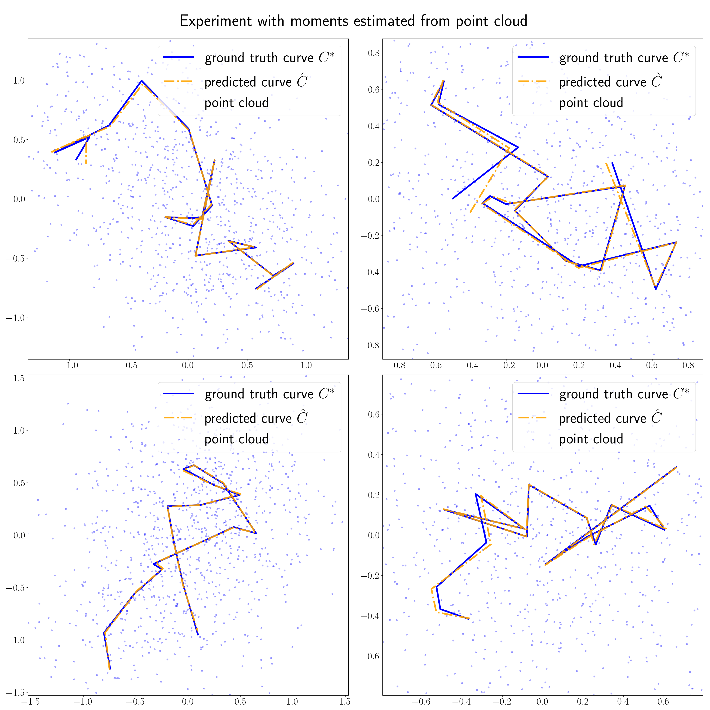
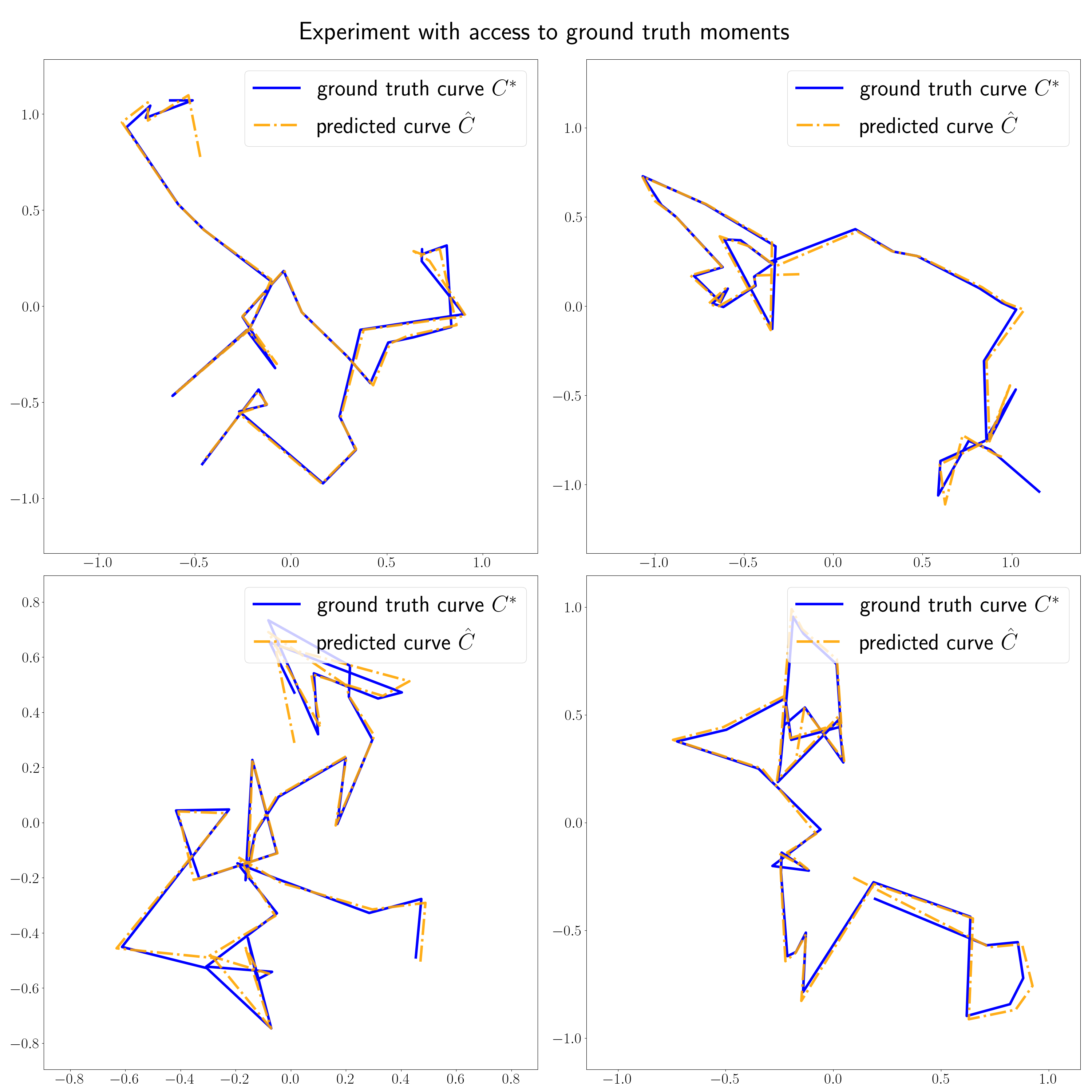
In Table 2, we present results from the experiment with moments estimated from a point cloud with points, with segments, ambient dimension , and noise level . We report the lower quartile, median, and upper quartile of the curve loss (see (3.1)) and third moment loss between the ground truth and predicted curves over 500 trials with different random ground truth curves . We present the results for the outputs of both phases of Algorithm 3, as well as the performance of both baselines with the best result out of random initializations. In Table 2, we present the same statistics for the experiment with access to ground truth moments with , and (we are able to perform the experiment in higher dimensions because we no longer have to generate and compute moments of a large point cloud, which is the primary performance bottleneck). We see that in both experiments, Algorithm 3 significantly outperforms both baselines in the curve loss, even without the finetuning phase. Observe also that the actual third moment loss is lower for the baseline algorithms even though the curve loss is higher; this indicates that the baseline algorithms are converging to a curve different from the ground truth . In the experiment with access to ground truth moments, the sorting of subspaces was successful times, where we define success as there being exactly one palindromic pair of sorted subspaces. In the experiment with moments estimated from a point cloud, the success rate was . We show some predicted curves from Algorithm 3 for both experiments in Figures 4 and 5.
7. Conclusion and Future Work
In this paper, we consider the problem of resolving a PWL constant speed curve in high dimensions from a high noise point cloud around the curve. We show that for sufficiently large noise, any algorithm hoping to recover the underlying curve with high probability will require at least samples, giving an asymptotic lower bound on the sample complexity. We then show that this lower bound is asymptotically tight by providing a recovery algorithm based on the third moment tensor, exploiting the fact that the third moment uniquely determines a curve in some neighborhood. Further work is needed in showing theoretical guarantees for our algorithm, e.g., showing robustness in the presence of error in the estimation of the curve moments from the data, or guarantees on Algorithm 2. There is also work to be done in recovery of curves other than PWL curves, as well as investigating the phase transition between the low noise and high noise recovery problems.
Acknowledgements
PL is partially funded by DE-SC0022232. YK is partially funded by DMS-2339439 and DE-SC0022232.
PL would like to thank Christopher Stith for enlightening discussions on the differential geometry arguments used in the proof of Proposition 3.2. YK would like to thank Xin Tong and Wanjie Wang from the National University of Singapore for discussions regarding the potential usage of moments in recovering a curve.
| curve loss | third moment loss | |||||
| method | 25% | 50% | 75% | 25% | 50% | 75% |
| Algorithm 3 after first phase | 0.2094 | 0.2368 | 0.2950 | 0.0573 | 0.0826 | 0.1279 |
| Algorithm 3 after second phase | 0.0516 | 0.0690 | 0.0997 | 0.0703 | 0.1609 | 0.3868 |
| Baseline algorithm with third moment only | 2.5430 | 2.8023 | 3.0430 | 0.0068 | 0.0107 | 0.0176 |
| Baseline algorithm with all three moments | 2.4590 | 2.7242 | 2.9343 | 0.0042 | 0.0060 | 0.0080 |
| curve loss | third moment loss | |||||
| method | 25% | 50% | 75% | 25% | 50% | 75% |
| Algorithm 3 after first phase | 0.4602 | 0.6363 | 0.9750 | 0.3066 | 0.8877 | 3.1077 |
| Algorithm 3 after second phase | 0.2054 | 0.4081 | 1.1064 | 0.7993 | 2.1035 | 11.3911 |
| Baseline algorithm with third moment only | 3.9449 | 4.2186 | 4.4786 | 0.0437 | 0.0725 | 0.1012 |
| Baseline algorithm with all three moments | 3.9404 | 4.1868 | 4.4431 | 0.0264 | 0.0347 | 0.0477 |
Appendix A Cloud Tracing Algorithm for the Low-Noise Regime
In this section, we very briefly outline our algorithm for tracing through low-noise point clouds. We do not perform any large-scale experiments or detailed analysis of the method.
For simplicity, we consider point clouds coming from a PWL curve with an a priori known constant segment lengths . First consider the issue of resolving an “elbow” with three points, , where is known. Since noise is low, we can compute the point cloud local to this elbow by considering all points in the cloud within distance of . The two-dimensional subspace formed by the three points can be estimated from the second empirical moment, onto which we can project the local point cloud. The direction (which we can identify with an angle in the two-dimensional subspace) of each vector pointing from to a projected point from the local cloud can be computed. The histogram of angle counts should be bimodal, with the peaks and occurring at the directions in which the projections of and lie. Since the segment lengths are known, we can then estimate the projections of and and deproject back to .
Given a full curve and an estimate of , we can first compute the point cloud local to , that is, all points that are within distance away from . We can apply a similar technique as above on this local cloud and to get an estimate for , then iteratively apply the elbow resolution technique to the elbow centered at and the point cloud local to to estimate . To account for the error that might propagate at each step, we can average the two curves obtained by applying this method with and as the starting points. Figure 2 shows the outcome of this method on curves in applied to only the initial point .
The reason why this method fails for the high noise case is that the local point clouds are no longer meaningful. When noise is low, the points within distance of have a high likelihood of coming from the elbow given by , , and , and so the geometric structure of the curve around is preserved by the local cloud. When noise is sufficiently high, the points within distance of are likely to have come from elsewhere in the curve. Without performing further detailed analysis, note that since this algorithm only requires accurate estimation of the second moment, the number of points needed for this method to work is order , rather than the requirement of to accurately estimate the third moment for our high noise recovery algorithm.
Appendix B Proof of Proposition 3.2
Let and be the first two moments of , let be the proportional segment lengths of , and let be the total length of . Then , , is one particular solution to the following system of polynomial equations in , , that we can write down using the relaxed moment expressions in (2.9):
| (B.1) | ||||
The first line in (B.1) is matching the relaxed first moment from and to the prescribed first moment , and similarly for the second line and the second moment . The third line “unrelaxes” the relaxed moments by requiring that the are equal to the proportional segment lengths, and the fourth line ensures that is equal to the length of the full curve.
The first line of (B.1) consists of equations, the second line consists of equations ( is a symmetric matrix, so we can eliminate all equations coming from the lower triangular part of ), the third line consists of equations, and the last line is a single equation, so we have a total of equations. To count the number of variables, we have variables from , variables from , and one variable from for a total of variables. We therefore have more variables than equations, and hence this is an underdetermined system of polynomial equations.
If we subtract the right hand side from both sides of each line of (B.1), we can consider the left hand side of the entire system as a function of (where scalars, vectors, and matrices are flattened and concatenated appropriately), and we can think of the solution set to (B.1) as the preimage of under .
Let be the Jacobian of in the variables , , and ; this is a short and wide matrix. In the next proposition, we claim that for almost all satisfying (B.1), the matrix is full rank.
Proposition B.1.
Let be a solution to (B.1) and suppose is not full rank. Then the all ones vector must be in the image of , where here we are thinking of as a matrix.
We omit the proof, which consists of routine calculation of the total derivative of . Since is a tall matrix with shape , its image must be rank deficient, and therefore is not in the image of for almost all . Therefore, for almost all , is full rank. Since rank is lower semicontinuous, for such a there exists a neighborhood of where is full rank and hence surjective at all in . Let be the restriction of to . Then is a regular value of , i.e., a point such that is surjective at every point in . Note that we know that is nonempty, since it contains at least the point . Then by the regular level set theorem from differential topology (also called the preimage theorem, see Theorem 9.9 in [25]), is a submanifold of with dimension . In other words, is not an isolated point in the real algebraic variety of (B.1). Therefore, for sufficiently small , we can find some such that and also solves (B.1), and hence has the same first and second moments as .
Appendix C Proof of Proposition 3.4
Our proof is modeled on the proof of Theorem A.1 in [21]. The idea of the proof is to bound the divergence with a Taylor series of the differences of moments. We first need to prove a few technical lemmas and introduce some notation. Let denote the density of a Gaussian centered at the origin with covariance :
| (C.1) |
Let denote the density of the noisy curve . Note that we have the expression
| (C.2) |
Here is a normalizing constant dependent on ; for the rest of this section, we will assume for notational simplicity. We will also be using the facts that is mean zero and throughout.
Lemma C.1.
We have the lower bound
| (C.3) |
Proof.
Using the fact that the exponential function is convex, we compute
The penultimate line is by Jensen’s inequality, and the last line is by the fact that is mean zero. ∎
Lemma C.2.
Let and be any two curves. Then
| (C.4) |
Proof.
Note that we have
and similarly for . Then
In line 4, we are using Fubini’s theorem and completing the square. ∎
Lemma C.3.
Let , be parametric curves such that and for all . With as defined in (3.1), we have the upper bound
| (C.5) |
Proof.
We are now ready to prove Proposition 3.4.
Proof (of Proposition 3.4).
Appendix D Vectorized Notation for Moments
Here we elaborate on the notation in Definition 2.10. We use , , and to denote the following three -shaped matrix constants (here for illustrative purposes):
| (D.1) |
( stands for sum, for left, and for right, since the rows of are , the rows of are , and the rows of are ). The -shaped matrix is given by
| (D.2) |
We use to denote the symmetric -shaped tensor whose entry is given by
| (D.3) |
Appendix E Miscellaneous Technical Lemmas
In this section, we collect miscellaneous technical lemmas and information-theoretic facts.
Lemma E.1.
Let , . Suppose also that we have . Then for any , we have the bound
| (E.1) |
The proof is adapted from the proof of Lemma B.12 in [3].
Proof.
Let . Note . Observe that we can write
By the binomial theorem,
In the third line from the bottom we are using the fact that the sum of the binomial coefficients is equal to . ∎
Definitions E.2.
Let and be the densities of two measures and that are absolutely continuous with respect to the Lebesgue measure. The divergence, divergence, and distance are defined as
In the definition of the norm, the supremum is over all measurable sets.
Lemma E.3.
We have the bound
| (E.2) |
Proof.
This is an immediate consequence of the fact that . ∎
Lemma E.4 (Pinsker’s Inequality, Lemma 2.5 in [24]).
For any two measures and ,
| (E.3) |
Lemma E.5.
Let and be random variables and and denote the distribution of independent draws from and . Then .
Proof.
For notational clarity, we only prove the case where . Then
∎
Lemma E.6.
Assume that are in generic position so that any collection of of the ’s is linearly independent. Let be the matrix given by
Then is a linearly independent set.
Proof.
We want to show that if , then for all . We can reindex the sum to write
| (E.4) |
For , let be a vector in such that for all . Let denote the tensor contraction along the last index of . Then kills a large number of terms and we have
We can rewrite this as , where
By our assumption of genericness, are linearly independent. Note also that is not in the span of and by our definition of . Therefore, if the linear combination of the four terms above is to be zero, that means we must have . Our genericness assumption also implies that and are nonzero. Note also that all are nonzero (positive, in fact). Therefore, if , then it must follow that and . Repeat this for . Then if , then (E.4) becomes
We’ve thus reduced our problem to whether is a linearly independent set.
Consider the sum
| (E.5) |
where are scalars. We can rewrite this as
| (E.6) |
Suppose for the sake of contradiction that (E.6) is equal to zero and not all are equal to zero; assume without loss of generality that is nonzero. Since are linearly independent, the summation is rank , where is the number of nonzero coefficients , so (E.6) is the sum of a rank 1 and rank matrix. If , then this sum cannot possibly be zero. If , suppose without loss of generality that is the only nonzero coefficient among , so that . Then must be parallel to , but this is not possible by our assumption that are generic. ∎
References
- [1] Anima Anandkumar, Rong Ge, Daniel Hsu, Sham M. Kakade, and Matus Telgarsky. Tensor decompositions for learning latent variable models, November 2014. arXiv:1210.7559.
- [2] Jonathan E. Atkins, Erik G. Boman, and Bruce Hendrickson. A spectral algorithm for seriation and the consecutive ones problem. SIAM Journal on Computing, 28(1):297–310, 1998.
- [3] Afonso S. Bandeira, Philippe Rigollet, and Jonathan Weed. Optimal rates of estimation for multi-reference alignment, May 2018. arXiv:1702.08546.
- [4] Mathieu Blondel, Quentin Berthet, Marco Cuturi, Roy Frostig, Stephan Hoyer, Felipe Llinares-López, Fabian Pedregosa, and Jean-Philippe Vert. Efficient and modular implicit differentiation, October 2021. arXiv:2105.15183.
- [5] James Bradbury, Roy Frostig, Peter Hawkins, Matthew James Johnson, Chris Leary, Dougal Maclaurin, George Necula, Adam Paszke, Jake VanderPlas, Skye Wanderman-Milne, and Qiao Zhang. JAX: composable transformations of Python+NumPy programs, 2018.
- [6] Charles Fefferman, Sergei Ivanov, Yaroslav Kurylev, Matti Lassas, and Hariharan Narayanan. Fitting a putative manifold to noisy data. In Proceedings of the 31st Conference On Learning Theory, volume 75 of Proceedings of Machine Learning Research, pages 688–720. PMLR, July 2018.
- [7] Charles Fefferman, Sergei Ivanov, Matti Lassas, and Hariharan Narayanan. Fitting a manifold to data in the presence of large noise, December 2023. arXiv:2312.10598.
- [8] Charles Fefferman, Sanjoy Mitter, and Hariharan Narayanan. Testing the manifold hypothesis. Journal of the American Mathematical Society, 29(4):983–1049, February 2016.
- [9] Fajwel Fogel, Alexandre d'Aspremont, and Milan Vojnovic. Serialrank: Spectral ranking using seriation. In Z. Ghahramani, M. Welling, C. Cortes, N. Lawrence, and K.Q. Weinberger, editors, Advances in Neural Information Processing Systems, volume 27. Curran Associates, Inc., 2014.
- [10] Alan E. Gelfand. Seriation methods for archaeological materials. American Antiquity, 36(3):263–274, July 1971.
- [11] Steven J. Gortler, Alexander D. Healy, and Dylan P. Thurston. Characterizing generic global rigidity, 2010. arXiv:0710.0926.
- [12] Björn Holmquist. Moments and cumulants of the multivariate normal distribution. Stochastic Analysis and Applications, 6(3):273–278, January 1988.
- [13] Yuehaw Khoo, Xin T. Tong, Wanjie Wang, and Yuguan Wang. Temporal label recovery from noisy dynamical data, 2024. arXiv:2406.13635.
- [14] Boris Landa and Xiuyuan Cheng. Robust inference of manifold density and geometry by doubly stochastic scaling. SIAM Journal on Mathematics of Data Science, 5(3):589–614, July 2023.
- [15] Roy R. Lederman, Joakim Andén, and Amit Singer. Hyper-molecules: on the representation and recovery of dynamical structures for applications in flexible macro-molecules in cryo-em. Inverse Problems, 36(4):044005, March 2020.
- [16] Marina Meilă and Hanyu Zhang. Manifold learning: What, how, and why. Annual Review of Statistics and Its Application, 11:393–417, April 2024.
- [17] Boris Mityagin. The zero set of a real analytic function, 2015. arXiv:1512.07276.
- [18] Kitty Mohammed and Hariharan Narayanan. Manifold learning using kernel density estimation and local principal components analysis, September 2017. arXiv:1709.03615.
- [19] Amit Moscovich, Amit Halevi, Joakim Andén, and Amit Singer. Cryo-em reconstruction of continuous heterogeneity by Laplacian spectral volumes. Inverse Problems, 36(2):024003, January 2020.
- [20] João M. Pereira, Joe Kileel, and Tamara G. Kolda. Tensor moments of Gaussian mixture models: Theory and applications, March 2022. arXiv:2202.06930.
- [21] Amelia Perry, Jonathan Weed, Afonso S. Bandeira, Philippe Rigollet, and Amit Singer. The sample complexity of multireference alignment. SIAM Journal on Mathematics of Data Science, 1(3):497–517, 2019.
- [22] Philippe Rigollet and Jonathan Weed. Uncoupled isotonic regression via minimum Wasserstein deconvolution. Information and Inference: A Journal of the IMA, 8(4):691–717, April 2019.
- [23] Amit Singer and Fred J. Sigworth. Computational methods for single-particle electron cryomicroscopy. Annual Review of Biomedical Data Science, 3(1):163–190, July 2020.
- [24] A. B. Tsybakov. Introduction to Nonparametric Estimation. Springer, 2009.
- [25] Loring W. Tu. An Introduction to Manifolds. Springer New York, second edition, 2011.
- [26] Dayang Wang, Feng-Lei Fan, Bo-Jian Hou, Hao Zhang, Zhen Jia, Boce Zhou, Rongjie Lai, Hengyong Yu, and Fei Wang. Manifoldron: Direct space partition via manifold discovery, May 2022. arXiv:2201.05279.
- [27] Hau-Tieng Wu. Design a metric robust to complicated high dimensional noise for efficient manifold denoising, January 2024. arXiv:2401.03921.
- [28] Zhigang Yao and Yuqing Xia. Manifold fitting under unbounded noise, June 2024. arXiv:1909.10228.