An anisotropic plasma model of the heliospheric interface

Abstract

We present a pioneering model of the interaction between the solar wind and the surrounding interstellar medium that includes the possibility of different pressures in the directions parallel and perpendicular to the magnetic field. The outer heliosheath region is characterized by a low rate of turbulent scattering that would permit a development of pressure anisotropy. The effect is best seen on the interstellar side of the heliopause, where a narrow region is developed with an excessive perpendicular pressure resembling a plasma depletion layer typical of planetary magnetspheres. The magnitude of this effect is relatively small owing to the fact that proton-proton collisions don’t permit the anisotropy to approach a stability threshold. We also show that if turbulence in the interstellar medium is weak, a much broader anisotropic boundary layer can exist, with a dominant perpendicular pressure in the southern hemisphere and a dominant parallel pressure in the north.

1 Introduction

The heliopause (HP) is the plasma boundary of the solar system, a separatrix layer between the cold, partially ionized and strongly magnetized local interstellar medium (LISM) and the warm inner heliosheath (IHS, the region between the termination shock and the HP). The existence of the heliopause, long since predicted by theory (Parker, 1961; Axford et al., 1963) and computer simulations (Baranov & Malama, 1993; Pauls et al., 1995; Pogorelov & Matsuda, 1998), is now firmly established by in situ observations by NASA’s Voyager 1 and Voyager 2 deep space probes that encountered the magnetic shear layer characteristic of the heliopause at heliocentric distances of 122 and 119 au, respectively (Burlaga et al., 2013, 2019). The outer heliosheath (OHS), a boundary layer between the HP and the bow wave, was found to have a plasma number density of the order of 0.1 cm^-3, which is about a factor of $\sim 50$ larger than in the inner heliosheath (Gurnett et al., 2013), and a magnetic field of between 4 and 7 $\mu$G – two to three times stronger than the field on the solar side of the HP (Burlaga et al., 2022).

Voyager 1 does not have a functioning plasma instrument, and the plasma density in the OHS was inferred from electrostatic oscillations thought to be produced by electron beams ahead of propagating shocks (Gurnett & Kurth, 2019), and from weak thermal noise at the local plasma frequency (Burlaga et al., 2021). While the plasma instrument on board Voyager 2 is functional, it is not well suited to perform observations in the OHS because three of its four sensors are pointing in the solar direction (Bridge et al., 1977), where as the plasma flow in the OHS is most probably directed toward the Sun, and because the energy of the protons in the OHS in only a few eV, which is below the lower energy threshold of the instrument. Nonetheless, Richardson et al. (2019) were able to place a constraint on the plasma temperature at 30,000–50,000 K. This is substantially larger than $\sim$7000–9000 K, the temperature in the local interstellar medium (LISM), well upstream of the bow wave, inferred from neutral helium observations (Witte, 2004; McComas et al., 2015). Numerical models predict the temperature near the HP to lie in the range between between 15,000 K (Zieger et al., 2013) and 45,000 K (Fraternale et al., 2023).

Voyager 1 measurements beyond the HP showed a general tend of increasing plasma density with heliocentric distance. Gurnett & Kurth (2019) reported a twofold increase in density, from 0.06 cm^-3 to 0.12 cm^-3 over a distance of 24 AU. This observation is reminiscent of plasma depletion layers (PDLs) known to exist between a bow shock and magnetopause of a planet. As first suggested by Zwan & Wolf (1976), density depletion is a consequence of magnetic field compression near the nose of the magnetic boundary, causing squeezing out of the plasma towards the flanks. The opposite trends exhibited by magnetic field strength and density are characteristic of a slow magnetosonic wave. Using a resistive MHD magnetospheric model, Wang et al. (2004) showed that pressure gradients are primarily responsible for accelerating plasma parcels in the direction parallel to the magnetic field lines. PDLs were since experimentally discovered in magnetospheres of Mercury (Gershman et al., 2013), Earth (Phan et al., 1994), Mars (Øieroset et al., 2004), Jupiter (Tsurutani et al., 1993), Saturn (Masters et al., 2014), and Neptune (Jasinski et al., 2022).

A distinguishing feature of a PDL is a decrease in parallel pressure $p_{\parallel}$ compared with perpendicular pressure $p_{\perp}$ owing to ions with large parallel velocity component escaping the compression region along the field lines leaving the gyrating ions behind. Under such conditions magnetic mirroring becomes the predominant effect pushing the plasma away from the region of strongest magnetic field (Denton & Lyon, 1996). Large values of the pressure anisotropy could lead to mirror or ion cyclotron instability development, and both modes were identified experimentally (Anderson & Fuselier, 1993; Violante et al., 1995).

Cairns & Fuselier (2017) argued, based on measured Voyager 1 density and magnetic field profiles beyond the HP, that the probe traversed a PDL with a width of 2.6 AU and a depletion factor of 2. Using a global MHD model of the heliosphere, Pogorelov et al. (2017) predicted that the plasma density would continue to increase for at least 100 au beyond the HP. This effects, however, is not produced by magnetic forces, but by charge exchange with interstellar neutral atoms. Furthermore, pressure anisotropy is expected to become smaller owing to Coulomb collisions, which are relatively frequent in the OHS, at least compared with the helioosphere. Fraternale & Pogorelov (2021) estimated the mean free path for proton collisions at $\sim 4$ au and decreasing with heliocentric distance. It is therefore expected that the heliospheric PDL, if it exists, should be relatively narrow, not exceeding a few au in width.

A direct modeling of the global heliospere with an anisotropic pressure tensor has never been attempted. The simplest fluid model that allows for temperature anisotropy is the Chew-Goldberger-Low (CGL) double-adiabatic model (Chew et al., 1956). Numerous CGL numerical models were developed in the past three decades to study the magnetospheres of Earth and other planets (Erkaev et al., 1999; Samsonov et al., 2001; Hu et al., 2010; Meng et al., 2012). Recently, a new CGL model with improved treatment of non-conservative terms and the isotropization process was developed by Bhoriya et al. (2024). The purpose of this paper is to apply that model to the heliospheric interface in order to elucidate the possible pressure anisotropies ahead of the HP on the LISM side of the interface. The numerical model presented here draws on our extensive work with geodesic meshes that constitute an efficient framework for modeling of astrophysical systems with a strong degree of central symmetry (Balsara et al., 2019; Florinski et al., 2020).

2 Double adiabatic MHD model

The CGL system of equations is obtained from the Boltzmann equation under the assumption of gyrotropy in the electric drift frame via an expansion in $r_{g}/L\ll 1$, where $r_{g}$ is the Larmor radius, and $L$ is a characteristic spatial scale of the problem (Chew et al., 1956). Unlike ideal (isotropic) MHD, the pressure tensor has two distinct components in the directions parallel ($p_{\parallel}$) and orthogonal ($p_{\perp}$) to the magnetic field $\mathbf{B}$. In a fixed inertial coordinate frame the pressure tensor has the form

$$\mathbf{p}=p_{\perp}\mathbf{I}+(p_{\parallel}-p_{\perp})\mathbf{bb},$$ (1)

where $\mathbf{b}=\mathbf{B}/B$ is the unit vector in the direction of the magnetic field. The resulting system of equations has five physical variables (density $\rho$, velocity $\mathbf{u}$, parallel pressure $p_{\parallel}$, perpendicular pressure $p_{\perp}$, and magnetic field $\mathbf{B}$) and consists of nine scalar equations. It cannot be written in a strictly conservative form because of the exchange of the thermal energy $\mathcal{E}$ between the parallel and the perpendicular degrees of freedom. Following Bhoriya et al. (2024) we retain the MHD conservation laws for mass, momentum, energy (appropriately corrected to account for anisotropic pressure), and magnetic flux, and designate $p_{\parallel}-p_{\perp}$ as the extra non-conserved variable. With these assumptions the governing CGL equations are

$$\frac{\partial\rho}{\partial t}+\nabla\cdot(\rho\mathbf{u})=0,$$ (2)

$$\frac{\partial(\rho\mathbf{u})}{\partial t}+\nabla\cdot\left[\rho\mathbf{uu}+p_{\perp}\mathbf{I}+(p_{\parallel}-p_{\perp})\mathbf{b}\mathbf{b}-\frac{1}{4\pi}\left(\mathbf{B}\mathbf{B}-\frac{B^{2}}{2}\textbf{I}\right)\right]=0,$$ (3)

$$\frac{\partial\mathcal{E}}{\partial t}+\nabla\cdot\left\{\left(\mathcal{E}+p_{\perp}+\frac{B^{2}}{8\pi}\right)\mathbf{u}+\mathbf{u}\cdot\left[(p_{\parallel}-p_{\perp})\mathbf{b}\mathbf{b}-\frac{\mathbf{B}\mathbf{B}}{4\pi}\right]\right\}=0,$$ (4)

$$\frac{\partial(p_{\parallel}-p_{\perp})}{\partial t}+\nabla\cdot\left[(p_{\parallel}-p_{\perp})\mathbf{u}\right]+(2p_{\parallel}+p_{\perp})\mathbf{b}\cdot\nabla\mathbf{u}\cdot\mathbf{b}-p_{\perp}\nabla\cdot\mathbf{u}=-\frac{p_{\parallel}-p_{\perp}}{\tau},$$ (5)

$$\frac{\partial\mathbf{B}}{\partial t}-\nabla\times(\mathbf{u}\times\mathbf{B})=0.$$ (6)

The energy density in equation (4) is calculated as

$$\mathcal{E}=\frac{\rho u^{2}}{2}+\frac{p_{\parallel}}{2}+p_{\perp}+\frac{B^{2}}{8\pi}.$$ (7)

All equations are written in CGS units. The right hand side of equation (5) contains the relaxation term that models the isotropizing effects of wave-particle interactions and Coulomb collisions on a timescale $\tau$. In what follows we will use parallel and perpendicular plasma betas $\beta_{\parallel}$ and $\beta_{\perp}$ as the ratios between the respective proton pressure component and the magnetic pressure $B^{2}/(8\pi)$, i.e., the electron pressure is considered to be small. We define the pressure anisotropy as $A=p_{\perp}/p_{\parallel}$.

It is well known that a bi-Maxwellian plasma distribution is subject to several types of instabilities. The CGL theory predicts two instabilities, firehose and mirror, that are associated with the Alfvén and the slow magnetosonic waves, respectively (Kato et al., 1966). In kinetic theory these are replaced by magnetosonic firehose, Alfvén firehose, ion cyclotron, and mirror instabilities (Hellinger et al., 2006; Bale et al., 2009). A fluid model does not need to distinguish between these different modes, but only include the anisotropy thresholds. The following thresholds are commonly used in CGL models:

$$\mathrm{firehose:}\;\beta_{\parallel}>\beta_{\perp}+2,$$ (8)

$$\mathrm{mirror:}\;\beta_{\perp}>\frac{\beta_{\parallel}}{2}+\sqrt{\beta_{\parallel}\left(1+\frac{\beta_{\parallel}}{4}\right)}.$$ (9)

The CGL PDE system stops being physically realizable, i.e. hyperbolic and solvable on a computer, if the pressure anisotropy grows without bounds. The model used in this work features an “elastic fence” technique introduced earlier in Bhoriya et al. (2024). Its design is such that for most of the domain in which the PDE system is physically realizable it allows us to use the physical relaxation time. It is only when the pressure anisotropy closely approaches the limit that the anisotropy is safely pushed away from going beyond the bounds of physical realizability. The value of $\tau$ in the model is the timescale for pitch-angle scattering due to ambient turbulence and that of proton-proton collisions. For pitch-angle scattering we may take $\tau=D_{\mu\mu}^{-1}$, where

$$D_{\mu\mu}\simeq\frac{\pi}{2}\frac{\Omega^{2}}{vB^{2}}P(k_{\mathrm{res}}),$$ (10)

where $v$ is the velocity of a thermal proton, $\Omega$ is the cyclotron frequency, and $P(k_{\mathrm{res}})$ is the magnetic power spectral density (PSD) at the resonant wavenumber $k_{\mathrm{res}}\sim\Omega/v$, which follows from the quasi-linear theory of wave-particle interactions (e.g., Jokipii, 1966). Assuming the PSD is a power law with an index $\gamma$ in the wavenumber range between $l_{c}^{-1}$ (where $l_{c}$ corresponds to the outer scale or the correlation length of the turbulence that are typically closely related) and infinity, and that the magnetic variance in the inertial range is equal to $aB^{2}$, where $a\sim 0.1$, we may write

$$\tau_{\mathrm{scat}}=\frac{2}{\pi a\Omega}\left(\frac{l_{c}}{r_{g}}\right)^{\gamma-1}.$$ (11)

This expression has three variables: the magnetic field $B$, the correlation length $l_{c}$, and the thermal speed $v$ that enters into $r_{g}$. The value of the correlation length must be assumed. It is often inversely proportional to $B$ because a compression of the field also compresses the fluctuations normal to the field, which are predominant. Suppose then that

$$l_{c}=l_{c0}\frac{B_{0}}{B},$$ (12)

where $l_{c0}$ and $B_{0}$ are some reference values (that are different in different regions). Then, assuming $\gamma=5/3$, we can write equation (11) as

$$\tau_{\mathrm{scat}}=\frac{1}{\pi}\left(\frac{4m_{p}cl_{0}^{2}B_{0}^{2}}{e}\right)^{1/3}\frac{1}{B}\left(\frac{\rho}{p}\right)^{1/3},$$ (13)

where $m_{p}$ and $e$ are the proton mass and charge, respectively.

The collisional time scale for momentum transfer can be found in textbooks (e.g., Burgers, 1969); in the present notations it is

$$\tau_{\mathrm{coll}}=\frac{3m_{p}^{2}v^{3}}{8\sqrt{2\pi}ne^{4}\Lambda},$$ (14)

where $\Lambda\sim 20$ is the Coulomb logarithm. Both timescales depend on the environment; Table 1 lists their typical values at 30 au in the solar wind, at 100 au in the IHS, and at 130 au in the OHS.

Table 1: Characteristic pitch-angle scattering and proton-proton Coulomb collision timescales in the solar wind, the inner heliosheath, and the OHS.

	$n$, cm-3	T, K	$B$, $\mu$G	$\Omega$, s-1	$v$, km s-1	$r_{g}$, au	$l_{c}$, au	$\tau_{\mathrm{scat}}$, yr	$\tau_{\mathrm{coll}}$, yr
SW (30 au)	$6\times 10^{-3}$	$10^{4}$	1.5	0.014	13	$9\times 10^{-6}$	0.2	$7\times 10^{-4}$	4.6
IHS (90 au)	$10^{-3}$	$10^{5}$	1	0.01	40	$3\times 10^{-5}$	0.2	0.01	800
OHS (130 au)	0.1	$2\times 10^{4}$	5	0.05	18	$6\times 10^{-6}$	2000	2	0.7

Turbulent correlation lengths in the solar wind have been measured and modeled (Breech et al., 2008; Oughton et al., 2011), and the value used in Table 1 is in agreement with the published values. To our knowledge, no such results for the IHS exist, so we use the solar-wind values as the nearest approximation. The correlation length for the OHS is based on the work of Burlaga et al. (2018).

In the solar wind at 30 au, and to the lesser extent in the IHS, temperature equilibration is rapid because of strong wave-particle interactions; Coulomb collisions, by contrast, are infrequent and so should not affect the pressure anisotropy. In the OHS, however, collisional and scattering timescales are similar. In this work we set $\tau=\tau_{\mathrm{scat}}$ based on Table 1 in the entire heliosphere (solar wind and IHS). For the OHS and LISM, however, we explore a range of possible isotropization rates, including those from Table 1, but also using larger and smaller values of this parameter (see the next section). To distinguish between the regions, a common approach is to use indicator variables $\alpha_{i}$ that are set to certain values at the boundary where the respective flow originates. In this model two indicator variables $\alpha_{1}$ and $\alpha_{2}$ are used that are initialized with a value of 1 at the inner and the outer boundary, respectively. The variables are passively advected with the plasma flow using the equation

$$\frac{\partial(\rho\alpha_{i})}{\partial t}+\nabla\cdot(\rho\alpha_{i}\mathbf{u})=0.$$ (15)

One can then adopt a convention that values of $\alpha_{i}$ close to 1 (say $>0.9$) correspond to “pure” solar wind or pure LISM, while smaller values indicate that there is a possibility of both plasmas co-existing within a single numerical cell. More often than not such “mixing” is a consequence of a limited spatial resolution of the computational mesh. Most of the results on pressure anisotropy presented in this paper are restricted for the pure LISM region.

At present, the CGL model does not provide for coupling between protons and neutral hydrogen atoms via a charge exchange, which is an essential process in the solar wind-LISM interaction (Blum & Fahr, 1970; Holzer, 1972; Wallis & Dryer, 1976). Charge exchange controls the geometric shape of the termination shock, the widths of both the IHS and the OHS, and the bulk plasma temperature (Pauls et al., 1995; Izmodenov, 2000). To our knowledge, full energy and momentum charge exchange terms have not been calculated for a bi-Maxwellian ion distribution. The reader is therefore cautioned that the dimensions of the heliosphere and the shapes of the termination shock and heliopause in our single-fluid model might not agree with the models featuring neutral atoms using multi-fluid or fluid-kinetic descriptions (Alexashov & Izmodenov, 2005; Heerikhuisen et al., 2006).

3 Computational mesh, initial and boundary conditions

As described in Bhoriya et al. (2024), the governing system of equations is solved using second-order WENO reconstruction on a quadrilateral geodesic mesh, also known as a cube sphere (Ronchi et al., 1996). This mesh avoids the polar singularities of the spherical mesh and allows for a larger and more spatially uniform time step. Because of an absence of charge exchange, the inner boundary can be taken farther from the sun; we set the inner boundary at $r_{\mathrm{min}}=30$ au and the outer boundary at $r_{\mathrm{max}}=1000$ au. In the radial direction, the computational mesh consisted of 720 shells of variable width. Given a uniformly varying (index) variable $\xi$ that takes values between 0 and 1, the radial distance was computed as

$$r(\xi)=r_{\mathrm{min}}\left\{1+\left[\frac{r_{\mathrm{max}}}{r_{\mathrm{min}}}-1-C(e^{\alpha}-1)\right]\xi+C(e^{\alpha\xi}-1)\right\},$$ (16)

with the parameter

$$C=\left[\frac{r_{\mathrm{med}}}{r_{\mathrm{min}}}-1-\chi\left(\frac{r_{\mathrm{max}}}{r_{\mathrm{min}}}-1\right)\right][e^{\alpha\chi}-1-\chi(e^{\alpha}-1)]^{-1}.$$ (17)

One can infer that the mapping given by (16) results in an approximately uniform mesh between $r_{\mathrm{min}}$ and $r_{\mathrm{med}}$ followed by an exponentially rationed mesh at larger distances. The parameter $\chi$ gives the percentage of grid points that lie between $r_{\mathrm{min}}$ and $r_{\mathrm{med}}$, and $\alpha$ specifies how smooth the transition between the two regions is. In this paper we used $r_{\mathrm{med}}=250$ au, $\chi=0.4$ (40% of grid points within the uniform shell region), and $\alpha=10$. The mesh on the sphere consisted of 29,400 quadrilateral faces.

A common practice in the global heliospheric modeling community is to start a simulation from a configuration consisting of two concentric annular regions. In this approach the inner region between $r_{\mathrm{min}}$ and $r_{\mathrm{tr}}$ (where “tr” stands for “transition”) corresponds to the solar wind, and the outer region represents the LISM. The solar wind is described as a steady supersonic radial outflow, while the LISM is modeled as a uniform flow. The $z$ axis of the coordinate system used by the code is conventionally chosen to be parallel to the solar rotation axis $\hat{\mbox{\boldmath$\omega$}}$. The angle between the former direction and the LISM flow vector is close to $95^{\circ}$, which is often approximated as a right angle. The inflow direction is then chosen to be the $x$ axis. For the transition distance we took $r_{\mathrm{tr}}=150$ au.

The conditions in the solar wind are specified at 1 au and propagated to the inner boundary of the simulation using the assumption that the flow behaves adiabatically. The latter is, of course incorrect, owing to the production of the pickup ions by charge exchange that significantly increases the bulk temperature of the combined plasma flow. To account for this, a temperature far in excess of the actual temperature at 1 au must be specified. In this work we used $2\times 10^{7}$ K at 1 au, which translates to a little over $2\times 10^{5}$ K at 30 au, which is not too far off the New Horizons observations (McComas et al., 2017). The reference 1 au number density was 5 cm^-3, and the solar wind velocity was taken to be 450 km s^-2; these numbers were imposed at all latitudes meaning there was no distinction between the fast slow solar wind. The magnetic field was assumed to have a strength of $5$ nT and a winding angle of $45^{\circ}$ at 1 au in the solar equatorial plane; these values were propagated to $r_{\mathrm{min}}$ using the standard Parker solution (Parker, 1958). The heliospheric current sheet was not included in the simulation. This is justified because the real current sheet oscillates in latitude producing a pattern of magnetic sectors that is too fine to be resolved, especially in the heliosheath (Opher et al., 2012; Pogorelov et al., 2013). In addition, an inevitable numerical dissipation of magnetic field in the current sheet could lead to unphysically large values of the temperature anisotropy.

To ensure that the initial magnetic field, which is defined at the faces of the computational cells, is divergence-free, it is initializes through the vector potential $\mathbf{A}$ on the edges of the cell. The heliospheric magnetic field field consists of two parts. The first is a radial monopole field, necessarily permeating all space, whose vector potential has a singularity making it inconvenient for numerical use (see below). The second component is the azimuthal field, restricted to the inner region. This field is simply

$$\mathbf{B}_{\mathrm{int}}=\mp\sqrt{2}B_{1}\frac{r_{1}}{r^{2}}(\hat{\mbox{\boldmath$\omega$}}\times\mathbf{r}),$$ (18)

where the sign depends on the chosen magnetic polarity in the monopole model. The corresponding vector potential is

$$\mathbf{A}_{\mathrm{int}}=\mp\sqrt{2}B_{1}r_{1}\left\{\frac{\mathbf{r}}{r}+\frac{[(\hat{\mbox{\boldmath$\omega$}}\times\mathbf{r})\times\mathbf{r}]}{r^{2}}\right\}.$$ (19)

We remind the reader that in our notation $\hat{\mbox{\boldmath$\omega$}}=\hat{\mathbf{e}}_{z}$.

The initial analytic solution in the exterior region (between $r_{\mathrm{tr}}$ and $r_{\mathrm{max}}$) is that of an incompressible, potential flow around a solid sphere. The velocity vector is tangential to the surface of the sphere at $r=r_{\mathrm{tr}}$ and tend to a uniform state at $r\to\infty$. Thus $\rho_{\mathrm{ext}}=\rho_{\infty}$, $p_{\mathrm{ext}}=p_{\infty}$, where the “infinity” subscript refers to pristine interstellar values, and

$$\mathbf{u}_{\mathrm{ext}}=\left(1+\frac{r_{t}^{3}}{2r^{3}}\right)\mathbf{u}_{\infty}-\frac{3r_{t}^{3}}{2r^{5}}(\mathbf{u}_{\infty}\cdot\mathbf{r})\mathbf{r},$$ (20)

where $\mathbf{u}_{\infty}=-u_{\infty}\hat{\mathbf{e}}_{x}$ is the interstellar inflow vector. The interstellar magnetic field is several orders of magnitude stronger than the initial interior field at $r_{\mathrm{tr}}$, and the initial interaction between the two flows can create very strong discontinuities that could lead to unstable behavior of the CGL code, which is more sensitive to flow gradients that conventional MHD codes. For this reason we start with a tapered initial magnetic field

$$\mathbf{B}_{\mathrm{ext}}=\frac{B_{\infty}}{2}(1+\tanh\psi)\hat{\mathbf{b}},$$ (21)

where

$$\psi=\frac{\hat{\mathbf{n}}\cdot(\mathbf{r}-\mathbf{u}_{\infty}t)-r_{1/2}}{\delta}.$$ (22)

In equation (22) $\hat{\mathbf{n}}$ is a unit vector normal to the planes $B=\mathrm{const}$, $r_{1/2}$ is the distance from the origin to the plane where the field’s strength decreases to one half of its interstellar value, $t$ is time, and $\delta$ is the taper width. We used $r_{1/2}=225$ au and $\delta=15$ au. The corresponding exterior vector potential is

$$\mathbf{A}_{\mathrm{ext}}=\frac{B_{\infty}\delta}{2}[\psi+\log(\cosh\psi)](\hat{\mathbf{b}}\times\hat{\mathbf{n}}).$$ (23)

The numerical values of the pristine LISM parameters were: $B_{\infty}=3\;\mu$G, $n_{\infty}=0.1$ cm^-3, $T_{\infty}=7\times 10^{3}$ K, and $u_{\infty}=26$ km s^-1. The magnetic field made an angle of $140^{\circ}$ with the LISM flow direction and the BV plane (the plane containing the LISM flow velocity and magnetic field vectors) was tilted by $45^{\circ}$ relative to the meridional plane. These values are consistent with our current knowledge of the LISM properties (Zirnstein et al., 2016).

As mentioned earlier, the radial component of the solar magnetic field must span both inner and outer regions. This is acceptable because the field drops off rapidly with radial distance, and so it has virtually no effect on the field at the outer boundary. This field is simply

$$\mathbf{B}_{\mathrm{rad}}=\pm\sqrt{2}B_{1}\frac{r_{1}^{2}}{r^{3}}\mathbf{r}.$$ (24)

The “$+$” sign must correspond to the “$-$” sign in equation (18) and vice versa. There is no corresponding vector potential because the field is initialized directly on the faces of the grid cells.

At the inner boundary the uniform and steady solar-wind conditions were maintained in the ghost zones throughout the simulation. In the outer boundary’s ghost zones the expressions for the magnetic field and vector potential were updated in time according to equations (21) and (23) to account for the advection of the initial profile. In the tail region the so-called non-reflecting boundary conditions were used to accelerate the flow to the local fast magnetosonic speed (Pogorelov & Semenov, 1997). To simplify the problem we used the isotropic version of the boundary conditions based on the averaged pressure $p=(p_{\parallel}+2p_{\perp})/3$.

4 Heliospheric structure: MHD vs. CGL

A total of three simulations were performed using different values of the pressure relaxation parameter in the LISM region. In the first simulation the timescale $\tau_{\mathrm{scat}}$ was 100 times smaller than estimated in Table 14. This corresponds, essentially, to the isotropic MHD case. The second simulation used the nominal values, and the third used a relaxation time 10 times longer than nominal. The last case would correspond to a situation where the turbulence in the OHS was almost entirely two-dimensional (and therefore ineffective in scattering the particles), or where the temperature of the interstellar cloud surrounding the heliosphere was higher by a factor of about 5, so that the mean collision time was increased tenfold. Note that the LISM was recently shown to be highly inhomogeneous (Swaczyna et al., 2022). It is therefore likely that the heliosphere was exposed to very different interstellar conditions in the past. All simulations were run to at least 400 years, which should be sufficient to establish a nearly steady flow structure.

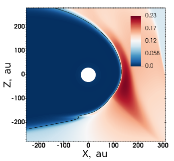
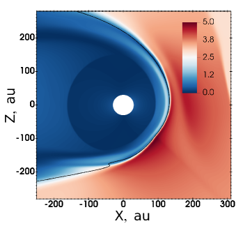
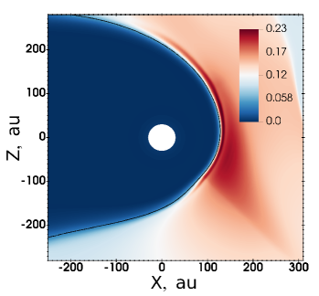
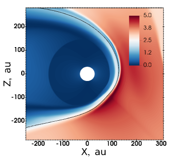
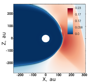
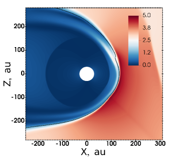
Figure 1: Plasma density $n$ in cm^-3 (left panels) and magnetic field strength $B$ in $\mu$G (right panels) in the meridional ($xz$) plane for the quasi-MHD (top), nominal (middle) and low (bottom) scattering rate. The figure was produced with VisIt software (Childs et al., 2012).

Figure 1 shows the plasma number density in the left panels and the magnetic field strength $B$ in the right panels, in the meridional plane, which is the plane containing the solar rotation axis and the LISM flow vector. In the density plots the red color corresponds to the LISM, while the less dense solar wind region is blue in color. The solid black line is the contour $\alpha_{2}=0.99$, which we treat as the definition of the heliopause. Note that only the forward (“nose”) portion of the heliosphere is shown in the figure; most of the heliotail is not covered by a high-resolution mesh so the differences between the models are not as dramatic.

The termination shock (easily discernible in the $B$ plots as a rapid change in color inside the heliospheric region) has a strong nose-tail asymmetry that is characteristic of models without neutral atoms. Note, however, that both the termination shock and HP are not fully stationary, but feature slowly evolving surface irregularities. It appears that, owing to the code’s absence of strong dissipation, major discontinuities such as the bow shock (which, the reader is reminded, is quite strong without the effects of plasma-neutral charge exchange) generate fluctuations in the flow that become incident on the HP causing small perturbations to its otherwise quasi-stationary structure. Note also that the color change at about $45^{\circ}$ (toward the lower right corner) is an artifact caused by the mesh imprint effect that is strongest near the vertices of the cube used as a template for the geodesic mesh (Florinski et al., 2020). A small portion of the bow shock is visible in the upper right corner of each image.

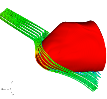
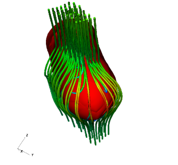
Figure 2: Magnetic field draping pattern around the “windward” part of the heliopause computed from the low scattering rate simulation. The red structure is the surface of the HP. Individual magnetic fields are shown as flux tubes with the color proportional to the magnetic field strength.

Figure 2 illustrates the draping of the magnetic field around the HP as viewed from the flank (left) and the front (right). The HP (shown in red) has a typical structure familiar from MHD models (Zirnstein et al., 2016; Izmodenov & Alexashov, 2020). The heliosphere is compressed in the direction perpendicular to the LISM magnetic field, and the structure is rotated relative to the BV plane. As discussed in Florinski et al. (2024), the magnetic field is strongest in the south where the flow pushes it against the HP, and weakest in the north, where the flow is more parallel to the field lines. As show below, these anisotropy should behave differently in these regions, $A>0$ in the south, and $A<0$ in the north.

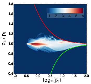
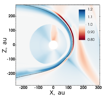
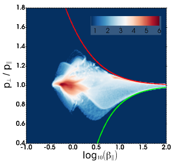
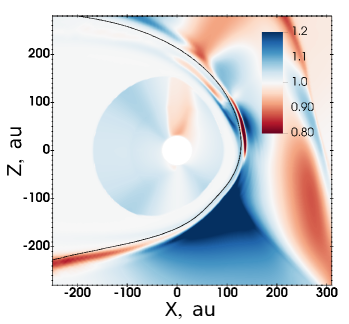
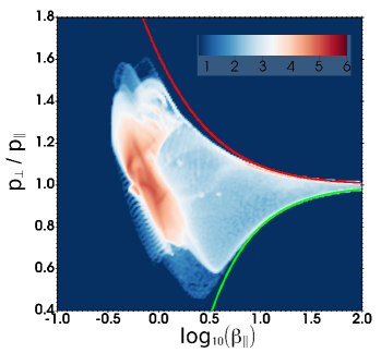
Figure 3: Pressure anisotropy $A$ in the meridional plane (left panels) and the binned distribution of the pressure anisotropy values vs. parallel plasma beta (right panels) for the quasi-MHD (top), nominal (middle) and low (bottom) scattering rate. The binned distributions were generated for the nose region defined by $\alpha_{2}>0.9$, $r<300$ au, $x>0$. The $A(\beta_{\parallel})$ distributions were weighted by the cell volume and use logarithmic color scale. The green lines refer to the firehose instability threshold given by equation (8) and the red lines refer to the mirror instability threshold, equation (9).

Figure 3 shows our results for the pressure anisotropy. The left panels show the expected increasing trend of $A$ with increased isotropization time from top to bottom. The MHD-like simulation (upper panel) is essentially isotropic, while the “standard” case has a narrow region of $A<1$ in the north. This result can be understood as follows. The magnetic field topology in that region is cusp-like, and the plasma flows mainly parallel to the field lines leading to a density increase; because the deformation is along the direction of $\mathbf{B}$, it leads to an increase in parallel pressure. The low-scattering simulation features a broad region with $A>0$ in the south. Here the plasma compression occurs primarily normal to the magnetic field lines, and an excess in $p_{\perp}$ develops. This feature bears a direct similarity with magnetospheric PDLs. We should point out, however, that because the system is only quasi-stationary, parcels of strongly anisotropic plasma in the nose can become advected toward the flanks and be replaced by upstream parcels with different values of $A$.

The frequency distribution of pressure anisotropy in the solar wind is conventionally presented on a $A(\beta_{\parallel})$ diagram (Bale et al., 2009; Hellinger et al., 2006). In a similar spirit, we present distributions of spatial locations with a given pressure ratio as a function of the parallel plasma beta. The right panels of Figure 3 shows the distributions for all three cases. Each was generated using $200\times 200$ bins using logarithmic bin spacing in $\beta_{\parallel}$ and linear spacing in the anisotropy. Because we are interested in the upwind OHS, and not in the IHS or the LISM region upstream of the bow shock (both of which are essentially isotropic), we restricted the binning algorithm to only count the cells that satisfy $\alpha_{2}>0.9$ (to exclude the heliosphere), $r<300$ au (to exclude the pre-bow-shock LISM) and, and $x>0$ (to exclude the tail region). The count rates were weighted by the cell volume. The dark red region corresponds to the “core” LISM plasma that is isotropic and has $\beta\sim 0.5$. As expected, the simulation with a hundredfold increase in the scattering rate has the anisotropy distribution that is strongly concentrated near the line $A=1$. The nominal and especially the low scattering rate simulations show much larger anisotropy variations in the OHS, ranging from $\sim 0.5$ and up to $1.6$. For the latter, the dark red “core” of the distribution is also spread between 0.8 and 1.2, which implies that most of the plasma in the upstream OHS exists in an asisotropic state. The red and green lines show the mirror and firehose instability thresholds, respectively (see equations 8 and 9); as expected the numerical results are contained to the left of these curves.

5 Discussion and conclusions

Every numerical study of the interaction between the solar system and its plasma environment to date was grounded in the assumption that the plasma distribution was isotropic in all space. This paper presents a major departure from this paradigm by allowing the interstellar plasma to develop a bi-Maxwellian distribution with distinctly different $p_{\parallel}$ and $p_{\perp}$. The anisotropy develops as a result of flow deformation in a directions parallel, perpendicular, or oblique to the magnetic field. A flow compression normal to the field leads to an increase in the perpendicular temperature as a result of conservation of magnetic moment. Conversely, a compression acting along the field lines tends to increase the parallel pressure owing to conservation of the longitudinal adiabatic invariant. Scattering on magnetic field fluctuations is the mechanism that prevents the plasma from developing prohibitively large anisotropies and crossing the stability threshold, which is forbidden in fluid models. The model used in this study demonstrated stable behavior under a very wide range of scattering rates.

Viewed on global scales, the interaction between the heliosphere and the LISM is not dramatically affected by the introduction of a pressure anisotropy. The flow and magnetic field draping patterns are quite similar in all three of our simulations, including the MHD-like. Plasma interactions with interstellar atoms and energetic particles (pickup ions and cosmic rays) could have a more pronounced effect on the structure (Fahr et al., 2000; Myasnikov et al., 2000). However, unlike MHD, the CGL model can tell us where pressure anisotropy driven instabilities are likely to occur and deduce the properties of the turbulence produced by these instabilities.

A common trend in the pressure anisotropy just beyond the HP is a development of a $A<1$ region in the northern hemisphere and a $A>1$ region in the south relatively to the solar equatorial plane. This behavior is fully consistent with the expectations based on $\mathbf{B}$ and the direction of deformation, as discussed above. This implies that plasma in the northern hemisphere could develop a firehose instability leading to a generation of Alfven or magnetosonic waves. Conversely, the southern hemisphere features a structure similar to a planetary plasma depletion layer, with a dominant perpendicular pressure component. We expect that mirror mode or ion cyclotron waves will be generated if the mirror instability threshold is crossed by the plasma. It is possible that these differences could be confirmed experimentally by comparing the compressibility of the turbulent magnetic fluctuations at Voyager 1 and Voyager 2 that are traveling in the northern and the southern hemispheres, respectively.

The lack of charge exchange in the model prevents us from making a quantitative comparison with the Voyager observations. For example, the LISM plasma density is the single fluid model is necessarily higher than measured; as a result the OHS plasma has a density of $\sim 0.2$ cm^-3, which is well in excess of the observed values. Charge exchange can, in principle, be treated with the isotropic model using the average pressure $p=(p_{\parallel}+2p_{\perp})/3$. Even in that case equation (5) would have to be modified to incorporate the effects of replacing protons taken from a bi-Maxwellian distribution with Maxwellian-distributed pickup ions. In our view, however, a framework built on an anisotropic plasma description should employ properly formulated anisotropic physics of charge exchange. This requires substantial additional theoretical development, and we leave it to future work.

While this work was focused on the OHS, there is some evidence that the IHS plasma is also anisotropic. Liu et al. (2007) argued that the plasma downstream of a quasi-perpendicular termination shock has $A>1$, and should be susceptible to a mirror instability. Tsurutani et al. (2011) and Burlaga & Ness (2011) interpreted the pressure-balanced structures (exhibiting anticorrelation between magnetic field strength and plasma density) observed by Voyager 1 in the IHS as mirror mode structures. Additionally, Fichtner et al. (2020) performed a calculation of anisotropy evolution based on quasi-linear interaction with the instability-generated mirror mode fluctuations in the IHS, starting from initially imposed values for $A$. The advantage of a CGL model is that the pressure anisotropy is provided as a part of the solution. However, we only include ambient magnetic fluctuations and ignore the possible instability-generated waves. Another physical aspect that is missing from the present model is the pickup process that tends to preferentially increase the perpendicular pressure of the bulk plasma in the IHS (in the nose direction), where the magnetic field is mainly perpendicular to the flow of interstellar neutral hydrogen. One can therefore envisage a two-fluid CGL model, where the pickup ions and the core thermal protons both have bi-Maxwellian distributions with different values of $A$.

References

- Alexashov & Izmodenov (2005) Alexashov, D. B., & Izmodenov, V. V. 2005, Astronomy and Astrophysics, 439, 1171–1181, doi: 10.1051/0004-6361:20052821
- Anderson & Fuselier (1993) Anderson, B. J., & Fuselier, S. A. 1993, Journal of Geophysical Research, 98, 1461–1479, doi: 10.1029/92JA02197
- Axford et al. (1963) Axford, W. I., Dessler, A. J., & Gottlieb, B. 1963, The Astrophysical Journal, 137, 1268–1278, doi: 10.1086/147602
- Bale et al. (2009) Bale, S. D., Kasper, J. C., Howes, G. G., et al. 2009, Physical Review Letters, 103, 211101, doi: 10.1103/PhysRevLett.103.211101
- Balsara et al. (2019) Balsara, D. S., Florinski, V., Garain, S., Subramanian, S., & Gurski, K. F. 2019, Monthly Notices of the Royal Astronomical Society, 487, 1283–1314, doi: 10.1093/mnras/stz1263
- Baranov & Malama (1993) Baranov, V. B., & Malama, Y. G. 1993, Journal of Geophysical Research, 98, 15157–15163, doi: 10.1029/93JA01171
- Bhoriya et al. (2024) Bhoriya, D., Balsara, D. B., Florinski, V., & Kumar, H. 2024, The Astrophysical Journal, 970, 154, doi: 10.3847/1538-4357/ad50a4
- Blum & Fahr (1970) Blum, P. W., & Fahr, H.-J. 1970, Astronomy and Astrophysics, 4, 280–290
- Breech et al. (2008) Breech, B., Matthaeus, W. H., Minnie, J., et al. 2008, Journal of Geophysical Research, 113, A08105, doi: 10.1029/2007JA012711
- Bridge et al. (1977) Bridge, H. S., Belcher, J. W., Butler, R. J., et al. 1977, Space Science Reviews, 21, 259–287, doi: 10.1007/BF00211542
- Burgers (1969) Burgers, J. M. 1969, Flow Equations for Composite Gases (New York and London: Acedemic Press)
- Burlaga et al. (2018) Burlaga, L. F., Florinski, V., & Ness, N. F. 2018, The Astrophysical Journal, 854, 20, doi: 10.3847/1538-4357/aaa45a
- Burlaga et al. (2021) Burlaga, L. F., Kurth, W. S., Gurnett, D. A., et al. 2021, The Astrophysical Journal, 911, 61, doi: 10.3847/1538-4357/abeb6a
- Burlaga & Ness (2011) Burlaga, L. F., & Ness, N. F. 2011, Journal of Geophysical Research, 116, A05102, doi: 10.1029/2010JA016309
- Burlaga et al. (2022) Burlaga, L. F., Ness, N. F., Berdichevsky, D. B., et al. 2022, The Astrophysical Journal, 932, 59, doi: 10.3847/1538-4357/ac658e
- Burlaga et al. (2019) —. 2019, Nature Astronomy, 3, 1007–1012, doi: 10.1038/s41550-019-0920-y
- Burlaga et al. (2013) Burlaga, L. F., Ness, N. F., & Stone, E. C. 2013, Science, 341, 147–150, doi: 10.1126/science.1235451
- Cairns & Fuselier (2017) Cairns, I. H., & Fuselier, S. A. 2017, The Astrophysical Journal, 834, 197, doi: 10.3847/1538-4357/834/2/197
- Chew et al. (1956) Chew, G. F., Goldberger, M. L., & Low, F. E. 1956, Proceedings of the Royal Society of London. Series A. Mathematical and Physical Sciences, 236, 112–118, doi: 10.1098/rspa.1956.0116
- Childs et al. (2012) Childs, H., Brugger, E., Whitlock, B., et al. 2012, in High Performance Visualization – Enabling Extreme-Scale Scientific Insight (Chapman and Hall/CRC), 357–372, doi: 10.1201/b12985
- Denton & Lyon (1996) Denton, R. E., & Lyon, J. G. 1996, Geophysical Research Letters, 23, 2891–2894, doi: 10.1029/96GL01590
- Erkaev et al. (1999) Erkaev, N. V., Farrugia, C. J., & Biernat, H. K. 1999, Journal of Geophysical Research: Space Physics, 104, 6877–6887, doi: 10.1029/1998JA900134
- Fahr et al. (2000) Fahr, H.-J., Kausch, T., & Scherer, H. 2000, Astronomy and Astrophysics, 357, 268–282
- Fichtner et al. (2020) Fichtner, H., Kleimann, J., Yoon, P. H., et al. 2020, The Astrophysical Journal, 901, 76, doi: 10.3847/1538-4357/abaf52
- Florinski et al. (2020) Florinski, V., Balsara, D. S., Garain, S., & Gurski, K. F. 2020, Computational Astrophysics and Cosmology, 7, 1, doi: 10.1186/s40668-020-00033-7
- Florinski et al. (2024) Florinski, V., Alonso Guzman, J. G., Kleimann, J., et al. 2024, The Astrophysical Journal, 961, 244, doi: 10.3847/1538-4357/ad0b15
- Fraternale & Pogorelov (2021) Fraternale, F., & Pogorelov, N. V. 2021, The Astrophysical Journal, 906, 75, doi: 10.3847/1538-4357/abc88a
- Fraternale et al. (2023) Fraternale, F., Pogorelov, N. V., & Bera, R. K. 2023, The Astrophysical Journal, 946, 97, doi: 10.3847/1538-4357/acba10
- Gershman et al. (2013) Gershman, D. J., Slavin, J. A., Raines, J. M., et al. 2013, Journal of Geophysical Research: Space Physics, 118, 7181–7199, doi: 10.1002/2013JA019244
- Gurnett & Kurth (2019) Gurnett, D. A., & Kurth, W. S. 2019, Nature Astronomy, 3, 1024–1028, doi: 10.1038/s41550-019-0918-5
- Gurnett et al. (2013) Gurnett, D. A., Kurth, W. S., Burlaga, L. F., & Ness, N. F. 2013, Science, 341, 1489–1492, doi: 10.1126/science.1241681
- Heerikhuisen et al. (2006) Heerikhuisen, J., Florinski, V., & Zank, G. P. 2006, Journal of Geophysical Research, 111, A06110, doi: 10.1029/2006JA011604
- Hellinger et al. (2006) Hellinger, P., Trávnic̆ek, P., Kasper, J. C., & Lazarus, A. J. 2006, Geophysical Research Letters, 33, L09101, doi: 10.1029/2006GL025925
- Holzer (1972) Holzer, T. E. 1972, Journal of Geophysical Research, 77, 5407–5431, doi: 10.1029/JA077i028p05407
- Hu et al. (2010) Hu, Y., Denton, R. E., & Lin, Y. 2010, Journal of Atmospheric and Solar-Terrestrial Physics, 72, 1155–1162, doi: 10.1016/j.jastp.2010.07.007
- Izmodenov (2000) Izmodenov, V. V. 2000, Astrophysics and Space Science, 274, 55–69, doi: 10.1023/A:1026579418955
- Izmodenov & Alexashov (2020) Izmodenov, V. V., & Alexashov, D. B. 2020, Astronomy and Astrophysics, 633, L12, doi: 10.1051/0004-6361/201937058
- Jasinski et al. (2022) Jasinski, J. M., Murphy, N., Jia, X., & Slavin, J. A. 2022, The Planetary Science Journal, 3, 76, doi: 10.3847/PSJ/ac5967
- Jokipii (1966) Jokipii, J. R. 1966, The Astrophysical Journal, 146, 480–487, doi: 10.1086/148912
- Kato et al. (1966) Kato, Y., Tajiri, M., & Taniuti, T. 1966, Journal of the Physical Society of Japan, 21, 765, doi: 10.1143/JPSJ.21.765
- Liu et al. (2007) Liu, Y., Richardson, J. D., Belcher, J. W., & Kasper, J. C. 2007, The Astrophysical Journal, 659, L65–L68
- Masters et al. (2014) Masters, A., Phan, T. D., Badman, S. V., et al. 2014, Journal of Geophysical Research: Space Physics, 119, 121–130, doi: 10.1002/2013JA019516
- McComas et al. (2015) McComas, D. J., Bzowski, M., Frisch, P., et al. 2015, The Astrophysical Journal, 801, 28, doi: 10.1088/0004-637X/801/1/28
- McComas et al. (2017) McComas, D. J., Zirnstein, E. J., Bzowski, M., et al. 2017, The Astrophysical Journal Supplement Series, 233, 8, doi: 10.3847/1538-4365/aa91d2
- Meng et al. (2012) Meng, X., Toth, G., Liemohn, M. W., Gombosi, T. I., & Runov, A. 2012, Journal of Geophysical Research: Space Physics, 117, A08216, doi: 10.1029/2012JA017791
- Myasnikov et al. (2000) Myasnikov, A. V., Alexashov, D. B., Izmodenov, V. V., & Chalov, S. V. 2000, Journal of Geophysical Research, 105, 5167–5177
- Øieroset et al. (2004) Øieroset, M., Mitchell, D. L., Phan, T. D., et al. 2004, Space Science Reviews, 111, 185–202, doi: 10.1023/B:SPAC.0000032715.69695.9c
- Opher et al. (2012) Opher, M., Drake, J. F., Velli, M., Decker, R. B., & Toth, G. 2012, The Astrophysical Journal, 751, 80, doi: 10.1088/0004-637X/751/2/80
- Oughton et al. (2011) Oughton, S., Matthaeus, W. H., Smith, C. W., Breech, B., & Isenberg, P. A. 2011, Journal of Geophysical Research, 116, A08105, doi: 10.1029/2010JA016365
- Parker (1958) Parker, E. N. 1958, The Astrophysical Journal, 128, 664–676, doi: 10.1086/146579
- Parker (1961) —. 1961, The Astrophysical Journal, 134, 20–27, doi: 10.1086/147124
- Pauls et al. (1995) Pauls, H. L., Zank, G. P., & Williams, L. L. 1995, Journal of Geophysical Research, 100, 21595–21604, doi: 10.1029/95JA02023
- Phan et al. (1994) Phan, T. D., Paschmann, G., Baumjohann, W., Sckopke, N., & Lühr, H. 1994, Journal of Geophysical Research: Space Physics, 99, 121–141, doi: 10.1029/93JA02444
- Pogorelov et al. (2017) Pogorelov, N. V., Heerikhuisen, J., Roytershteyn, V., et al. 2017, The Astrophysical Journal, 845, 9, doi: 10.3847/1538-4357/aa7d4f
- Pogorelov & Matsuda (1998) Pogorelov, N. V., & Matsuda, T. 1998, Journal of Geophysical Research, 103, 237–245, doi: 10.1029/97JA02446
- Pogorelov & Semenov (1997) Pogorelov, N. V., & Semenov, A. Y. 1997, Astronomy and Astrophysics, 321, 330–337
- Pogorelov et al. (2013) Pogorelov, N. V., Suess, S. T., Borovikov, S. N., et al. 2013, The Astrophysical Journal, 772, 2, doi: 10.1088/0004-637X/772/1/2
- Richardson et al. (2019) Richardson, J. D., Belcher, J. W., Garcia-Galindo, P., & Burlaga, L. F. 2019, Nature Astronomy, 3, 1019–1023, doi: 10.1038/s41550-019-0929-2
- Ronchi et al. (1996) Ronchi, C., Iacono, R., & Paolucci, P. S. 1996, Journal of Computational Physics, 124, 93–114, doi: 10.1006/jcph.1996.0047
- Samsonov et al. (2001) Samsonov, A. A., Pudovkin, M. I., Gary, S. P., & Hubert, D. 2001, Journal of Geophysical Research, 106, 21,689, doi: 10.1029/2000JA900150
- Swaczyna et al. (2022) Swaczyna, P., Schwadron, N. A., Möbius, E., et al. 2022, The Astrophysical Journal Letters, 937, L32, doi: 10.3847/2041-8213/ac9120
- Tsurutani et al. (2011) Tsurutani, B. T., Lakhina, G. S., Verkhoglyadova, O. P., et al. 2011, Journal of Geophysical Research, 116, A02103, doi: 10.1029/2010JA015913
- Tsurutani et al. (1993) Tsurutani, B. T., Southwood, D. J., Smith, E. J., & Balogh, A. 1993, Journal of Geophysical Research: Space Physics, 98, 21203–21216, doi: 10.1029/93JA02586
- Violante et al. (1995) Violante, L., Bavassano Cattaneo, M. B., Moreno, G., & Richardson, J. D. 1995, Journal of Geophysical Research: Space Physics, 100, 12047–12055, doi: 10.1029/94JA02703
- Wallis & Dryer (1976) Wallis, M. K., & Dryer, M. 1976, The Astrophysical Journal, 205, 895–899, doi: 10.1086/154345
- Wang et al. (2004) Wang, Y. L., Raeder, J., & Russell, C. T. 2004, Annales Geophysicae, 22, 1001–1017, doi: 10.5194/angeo-22-1001-2004
- Witte (2004) Witte, M. 2004, Astronomy and Astrophysics, 426, 835–844, doi: 10.1051/0004-6361:20035956
- Zieger et al. (2013) Zieger, B., Opher, M., Schwadron, N. A., McComas, D. J., & Tóth, G. 2013, Geophysical Research Letters, 40, 2923–2928, doi: 10.1002/grl.50576
- Zirnstein et al. (2016) Zirnstein, E. J., Heerikhuisen, J., Funsten, H. O., et al. 2016, The Astrophysical Journal, 818, L18, doi: 10.3847/2041-8205/818/1/L18
- Zwan & Wolf (1976) Zwan, B. J., & Wolf, R. A. 1976, Journal of Geophysical Research, 81, 1636–1648, doi: 10.1029/JA081i010p01636