Memory and Friction: From the Nanoscale to the Macroscale

Abstract

Friction is a phenomenon that manifests across all spatial and temporal scales, from the molecular to the macroscopic scale. It describes the dissipation of energy from the motion of particles or abstract reaction coordinates and arises in the transition from a detailed molecular-level description to a simplified, coarse-grained model. It has long been understood that time-dependent (non-Markovian) friction effects are critical for describing the dynamics of many systems, but that they are notoriously difficult to evaluate for complex physical, chemical, and biological systems. In recent years, the development of advanced numerical friction extraction techniques and methods to simulate the generalized Langevin equation have enabled exploration of the role of time-dependent friction across all scales. We discuss recent applications of these friction extraction techniques and the growing understanding of the role of friction in complex equilibrium and non-equilibrium dynamic many-body systems

1 Introduction

Many systems across a wide range of spatial and temporal scales, whether physical, chemical, biological, ecological, economic, financial, or meteorological, are many-body, interacting systems. Describing the dynamics of the individual parts is often computationally or experimentally impossible. Therefore, the focus is usually on the dynamics of a low-dimensional collective variable or reaction coordinate, typically influenced by the rest of the system not under direct observation. Examples include the motion of a tracer particle within a liquid [1, 2, 3, 4, 5, 6], the vibrational modes of a molecule in gas or liquid phases [7, 8, 9], the system polarization in spectroscopy [10, 11, 12], the shear strain as a function of shear stress in rheology experiments [13, 14], the distance between two fluorescently labeled amino acids in protein folding experiments [15, 16, 17, 18, 19], and the position of a moving organism in biological motility studies [20, 21, 22, 23]. Overall, the goal is to replace the full description of the many-body system with a low-dimensional observable and to derive accurate equations of motion that model the dynamics of that observable by coupling it with its environment’s dynamics.

[] ProjectionSystematic method to single out interesting parts of high-dimensional phase space in the form of a one- or low-dimensional observable Generalized Langevin equation (GLE)Non-Markovian equation of motion for describing the dynamics of a general stochastic observable Coarse grainingTechniques that reduce the number of degrees of freedom used to describe the structure and dynamics of a system Non-Markovian frictionFriction force that depends on the current and past velocities of an observable Memory kernelThe function $\Gamma(t)$ encapsulating time-dependent friction due to dissipative relaxation effects in the environment

The process of deriving the equation of motion for an arbitrary low-dimensional observable is known as projection [24, 25, 26, 27]. An appropriate observable that captures the system’s essential behavior or is experimentally measurable is selected, and then a projection operator is constructed to single out the dynamics of the observable while the remaining degrees of freedom form the environment. The result is a generalized Langevin equation (GLE), which features a memory-dependent friction, a potential of mean force term, and a complementary force term (typically called a random force), representing interactions with the environment. Note that there are many choices for the projection operator [25, 27, 28, 29, 30, 31, 32] that produce different GLEs, exact when no approximations are applied to the complementary force term. Although friction appears explicitly, the GLE is time-reversible if no additional approximations are made. The GLE parameters can be extracted from experimental or simulation time series data, and many techniques for extracting friction memory kernels are available [33, 34, 35, 36, 32]. Unavoidable data discretization in time can be addressed with refined estimation methods [37]. Overall, the GLE has emerged as a common and practical coarse-graining technique [38, 39, 40, 41].

In this review, we cover a broad range of topics where the effects of non-Markovian friction significantly influence the system dynamics. These include the free diffusion of particles and the motility of biological cells in complex environments, the motion of reaction coordinates in confining potentials and the dynamics of rare events, the folding of proteins, molecular vibrational spectroscopy, the dynamics of meteorological weather patterns, and more. We analyze these systems from the perspective of the GLE and discuss applying memory kernel extraction to evaluate friction and dissipation time scales. Additionally, we discuss Markovian embedding simulation techniques for efficient GLE simulation, parameterized using extraction techniques. These Markovian embedding techniques consist of transforming the GLE into a set of coupled ordinary Langevin equations that can be efficiently simulated to reproduce GLE dynamics. Perturbing model parameters near extracted values efficiently probes the friction and potential energy landscape’s influence on observable dynamics [42, 43]. In its original formulation, the GLE is not suitable for describing systems that are out of equilibrium in their stationary states. Living systems, such as cells and organisms, are examples of such truly non-equilibrium systems and have been intensely studied in recent years [44, 45, 46]. The formulation of GLEs for out-of-equilibrium systems is an active field of research [41, 47, 48], as we discuss briefly throughout the review.

This review is organized as follows. In Section 2, we provide an overview of systems that have recently been analyzed using the GLE and which exhibit significant non-Markovian friction effects. In Section 3, we provide a brief derivation of the GLE, memory-kernel extraction techniques, and the Markovian embedding framework for simulating GLEs. In Section 4, we present extracted memory-dependent friction kernels for three systems discussed in Section 2 and compare the system diffusivities. In Section 5, we describe three implications of the effects of memory-dependent friction on standard statistical mechanical observables. Finally, in Section 6, we describe three investigations based on the application of the GLE: protein folding at the nanoscale (Section 6.1), cell-type classification at the microscale (Section 6.2), and weather pattern prediction at the macroscale (Section 6.3).

[] Memory kernel extractionMethods to determine $\Gamma(t)$ from time series data Markovian embeddingMethod to transform the non-Markovian GLE into a set of coupled Markovian Langevin equations

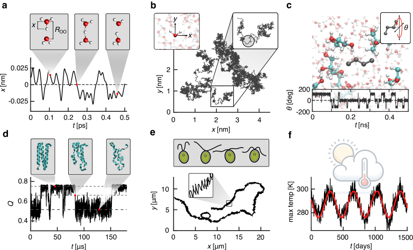
Figure 1: From nano to macro: dynamics across different spatial and temporal scales. (a) An ab initio molecular dynamics (MD) simulation of the proton-transfer reaction between two water molecules at a fixed relative distance of R${}_{\mathrm{OO}}=2.56\textup{~{}\AA}$. The reaction coordinate $x(t)$ represents the excess proton’s position along the oxygen-oxygen axis. [49]. (b) Classical MD simulation of the diffusion of a single water molecule in a liquid water environment, showing the 1 ns path of the oxygen atom in the $x,y$ plane. The magnification focuses on a 50 ps trajectory segment where the short-time-scale inertia- and memory-dominated dynamics can be observed (gray circle). (c) Isomerization dynamics of an n-butane molecule solvated in a mixed water-glycerol solvent (20$\%$ mass fraction glycerol), simulated using classical MD. The time evolution of the n-butane dihedral angle $\theta(t)$ is shown, as it transitions between distinct isomeric states. The composition of the complex solvent environment influences the dynamics of dihedral isomerization [50]. (d) The folding dynamics of the 73-residue $\alpha_{3}$D fast-folding protein. The fraction of native contacts reaction coordinate $Q(t)$ is a one-dimensional collective-coordinate representation of the full atomic structure of the protein, which transitions back and forth between folded and unfolded states. Representative molecular structures of a folded state and unfolded state, as well as a transition state, are shown [51]. (e) An 8-second swimming trajectory of the center of a Chlamydomonas reinhardtii algae cell. The illustrated stroke cycle takes approximately 25 ms, and the persistent oscillations from the stroking motion are visible in the magnification. On longer timescales, the cell executes a random walk [23]. (f) The daily maximal temperature in Berlin-Tegel is plotted over four years. The temperature exhibits large fluctuations on the daily time scale as well seasonal oscillations. Predicting daily temperature is of practical interest.

2 Examples of systems that are governed by non-Markovian friction

In Figure 1, we show an overview of different systems discussed throughout this review. These systems span the range from the nanoscopic scale of a quantum-chemical description of subatomic particle transport to the scale of biological cells, and up to the terrestrial scale of meteorological processes. In all of these examples, the application of GLE modeling and friction memory-kernel extraction has illuminated the underlying dynamics of the relevant observables, thereby enhancing our understanding of the holistic dynamics of these systems. Figure 1a illustrates the proton-transfer reaction between two water molecules at a fixed separation, obtained from ab initio molecular dynamics (MD) simulations. The dynamics of excess protons in water is important in chemistry and biology and plays a fundamental role in acid-base reactions, enzyme catalysis, and proton transport in biological membranes [52, 53]. This process exhibits a significantly higher diffusion coefficient than other ions in water. This distinct property is due to the Grotthuss mechanism, by which excess protons subsequently transfer between individual water molecules and exchange identities with other hydrogen nuclei within hydronium ions [53, 54, 55]. An elementary step in the long-distance diffusion of protons in water is therefore the barrier crossing between two water molecules [56, 57, 58, 59, 49]. In Figure 1b, we see the diffusive transport of a single water molecule in bulk liquid water. The trajectory reveals self-similarity, a characteristic of diffusion that breaks down below the picosecond scale, where inertia and memory effects dominate the molecular dynamics [60, 40, 61]. In Figure 1c and 1d, we highlight the importance of molecular conformation dynamics. In Figure 1c, the isomerization dynamics of a single dihedral bond in the n-butane molecule is strongly influenced by the complex mixed water-glycerol solvent environment. Simulations of n-butane, and other small, isomerizing molecules, are computationally inexpensive and provide an ideal system for investigating internal friction effects and the role of viscogenic coupling in small isomerizing molecules [36, 62, 50]. The folding and unfolding dynamics of the fast-folding $\alpha_{3}$D protein shown in Figure 1d, however, are significantly computationally expensive and such classical MD simulations require advanced special-purpose computers [63, 64]. The study of the friction acting on a folding protein has a long history, particularly due to the pronounced influence of internal friction on folding dynamics [65, 66, 67, 68, 69, 70, 71]. Extensive trajectories, like those in Figure 1d, provide a crucial testing ground to study memory friction effects in protein folding [51]. In Figures 1e and 1f, we emphasize systems at greater spatial and temporal scales. The swimming Chlamydomonas reinhardtii alga in Figure 1e must overcome strong hydrodynamic resistance to move through its fluid-medium environment. At short time scales, its motion is characterized by the periodic beating of its flagella. At longer time scales, it appears to execute undirected diffusive motion. The motion of organisms across multiple time scales has long been described using stochastic models [72, 73, 74, 75, 76], such as Lévy random walks [77, 78] and even GLEs [22, 79, 23]. In this review, we will discuss a novel application of the GLE as a classification scheme for determining modes of cellular motion. In Figure 1f, and in the final section of this review, we explore the terrestrial scale. Coarse graining is absolutely necessary for describing terrestrial phenomena, such as the atmosphere, economies, financial systems, or ecosystems, since it is impossible to explicitly model the myriad interacting agents in detail. Weather patterns, such as the daily maximal temperature measured at Berlin-Tegel, as presented in Figure 1f, follow long-term seasonal trends and short-term stochasticity. By filtering out the deterministic modes in the signal, the remaining stochastic process can be modeled by the GLE, which provides a framework for highly accurate daily temperature predictions with a fraction of the computational cost of machine-learning techniques.

3 Memory-dependent friction and the generalized Langevin equation (GLE)

This review discusses recent applications of the GLE as a coarse-graining tool for extracting and analyzing time-dependent friction memory kernels from time series data across various physical, chemical, and biological systems. In this section, we provide brief derivations of the GLE, the friction memory-kernel extraction method, and the Markovian embedding approach for simulating the GLE.

3.1 Derivation of the GLE: a sketch

The derivation of the GLE is based on the dynamics of a general many-body system that is fully characterized by the Hamiltonian ${\cal H}(R,P)$ in terms of the $3N$ particle, or atomic, positions $R$ and their $3N$ momenta $P$. The Liouville operator ${\cal L}(R,P)$, which depends on the Hamiltonian, gives the rate of change of an arbitrary phase-space-dependent observable $x(R,P,t)$ as $\dot{x}(R,P,t)={\cal L}(R,P)x(R,P,t)$. The solution of this differential equation can be formally written using the operator exponential as $x(R,P,t)=\exp(t{\cal L}(R,P))x(R,P,0)$, from which the acceleration of the observable is obtained by differentiation as $\ddot{x}(R,P,t)=\exp(t{\cal L}(R,P)){\cal L}^{2}(R,P)x(R,P,0)$. A crucial step in the derivation of the GLE is introducing a projection operator ${\cal P}$ to single out a relevant part of phase space, such as the observable $x(R,P,0)$ itself, its rate of change $\dot{x}(R,P,0)$, or a combination of both. Together with the complementary projection operator ${\cal Q}$, the identity operator $1={\cal P}+{\cal Q}$ is obtained, which defines ${\cal Q}$. The starting point of the derivation of the GLE is to insert this identity operator into the expression for the acceleration of the reaction coordinate according to

$$\begin{split}\ddot{x}(R,P,t)&=e^{t{\cal L}(R,P)}{\cal L}^{2}(R,P)({\cal P}+{\cal Q})x(R,P,0)\\ &=e^{t{\cal L}(R,P)}{\cal L}^{2}(R,P){\cal P}x(R,P,0)+e^{t{\cal L}(R,P)}{\cal L}^{2}(R,P){\cal Q}x(R,P,0),\end{split}$$ (1)

where in the last step, we used the fact that both the exponential and Liouville operators are linear. The acceleration $\ddot{x}(R,P,t)$ splits into two parts. The first is produced by the relevant projection operator ${\cal P}$ and gives rise to forces from the gradient of a conservative potential, as described by Newton’s equation of motion. The second part comes from the complementary projection operator ${\cal Q}$ and accounts for forces due to environmental interactions. After a few additional steps of manipulation, one arrives at the GLE in the general form [29, 30, 48]

$$\ddot{x}(t)=-\nabla\bar{U}\big{[}x(t)\big{]}-\int\limits_{0}^{t}\bar{\Gamma}(t-t^{\prime})\dot{x}(t^{\prime})dt^{\prime}+\bar{F}_{\text{R}}(t),$$ (2)

which consists of a potential gradient term $\nabla\bar{U}(x)$, a friction term with friction memory kernel $\bar{\Gamma}(t)$, and a complementary force $\bar{F}_{\text{R}}(t)$, which is often interpreted as a stochastic force. The force correlator approximately follows $\langle\bar{F}_{\text{R}}(t)\bar{F}_{\text{R}}(t^{\prime})\rangle=\langle\dot{x}^{2}\rangle\bar{\Gamma}(t-t^{\prime})$ [29, 30, 31, 80]. There are many different projection operators ${\cal P}$, which lead to different GLEs. For details, see [25, 26, 27, 29, 30, 31, 80]. Note that, in writing Eq. 2, we dropped the phase-space dependence of the observable $x(t)$ and the complementary force $\bar{F}_{\text{R}}(t)$. The overbar notation indicates a GLE formulation where no mass appears in front of the acceleration, which applies to both equilibrium and non-equilibrium systems. Consequently, the quantities $\bar{U}(x)$, $\bar{\Gamma}(t)$ and $\bar{F}_{\text{R}}(t)$ do not have their usual physical units.

For equilibrium systems, where a heat-bath temperature is defined, the equipartition theorem $m\langle\dot{x}^{2}\rangle=k_{\text{B}}T$ holds, allowing the introduction of an effective mass $m$, which is specific to the observable. Thus, Eq. 2 can be written in a standard equilibrium form [36, 60, 42, 81, 43, 51, 50]

$$m\ddot{x}(t)=-\nabla U\big{[}x(t)\big{]}-\int\limits_{0}^{t}\Gamma(t-t^{\prime})\dot{x}(t^{\prime})dt^{\prime}+F_{\text{R}}(t),$$ (3)

where the quantities ${U}(x)$, ${\Gamma}(t)$, and ${F}_{\text{R}}(t)$ have their usual physical units. Note that the mass $m$ and the friction kernel ${\Gamma}(t)$ can, in principle, depend on $x$ [29, 80], which is, however, not covered in this review. For simplicity, we only consider one-dimensional observables; generalizing to vectorial observables is possible and relevant but not explicitly discussed here. When discussing equilibrium systems throughout this review, we use Equation 3. For non-equilibrium systems, such as cellular motility (Sections 4 and 6.2) and meteorological processes (Section 6.3), we maintain the general form of Equation 2.

3.2 Extraction of the GLE parameters from time-series data

Recent advances in the study of memory-dependent friction effects in complex systems have become possible through the development of robust memory kernel extraction techniques [33, 36, 60, 42]. With sufficient time series data, the observable’s stochastic trajectory can be mapped onto a GLE, and a numerical representation for the friction memory kernel $\Gamma(t)$ is evaluated. In this section, we derive an extraction scheme for the GLE as given in Eq. 3.

Recently, techniques have focused on extracting the running integral of the memory kernel $G(t)$, defined as

$$G(t)=\int_{0}^{t}\Gamma(t^{\prime})dt^{\prime},$$ (4)

such that a distinct plateau identifies the friction coefficient, $\gamma$, for the observable, defined as $\gamma\equiv G(t\rightarrow\infty)$ [60, 42]. Equivalent methods can be used for directly extracting $\Gamma(t)$ [60, 36]. To extract a numerical approximation to $G(t)$, we multiply the generalized Langevin equation (GLE) in Eq. 3 by the initial velocity $\dot{x}(0)$ and evaluate the ensemble average, leading to the correlation function $C^{\dot{x}\ddot{x}}(t)=\big{\langle}\dot{x}(0)\ddot{x}(t)\big{\rangle}$. Since the random force in Eq. 3 lies in a subspace orthogonal to $\dot{x}(t)$ for all $t$, both $\big{\langle}\dot{x}(0)F_{\text{R}}(t)\big{\rangle}=0$ and $\big{\langle}{x}(0)F_{\text{R}}(t)\big{\rangle}=0$. Integrating the entire equation once, we arrive at the relationship

$$\frac{C^{\dot{x}\dot{x}}(t)}{C^{\dot{x}\dot{x}}(0)}C^{{x}\nabla U}(0)=C^{{x}\nabla U}(t)-\int_{0}^{t}G(t-t^{\prime})C^{\dot{x}\dot{x}}(t^{\prime})dt^{\prime},$$ (5)

see [42] for details.

Eq. 5 is expressed in terms of two correlation functions, $C^{\dot{x}\dot{x}}(t)=\big{\langle}\dot{x}(0)\dot{x}(t)\big{\rangle}$ and $C^{{x}\nabla U}(t)=\big{\langle}{x}(0)\nabla U\big{[}x(t)\big{]}\big{\rangle}$, both of which are easily evaluated from long time series trajectories. A key feature of this memory kernel extraction technique is that it applies generally to systems evolving across arbitrary free-energy landscapes $U(x)$. For the time series trajectories shown in Figures 1a, 1c, and 1d, the free energy profiles $U(x)$ are extracted using $U(x)=-k_{\text{B}}T\log\big{[}\rho(x)\big{]}$, where $\rho(x)$ is the probability density over $x(t)$, evaluated via histogram binning, and $\nabla U\big{[}x(t)\big{]}$ is constructed by interpolation. Eq. 5 can be discretized using the trapezoidal integration rule, leading to

$$\frac{C^{\dot{x}\dot{x}}_{i}}{C^{\dot{x}\dot{x}}_{0}}C^{{x}\nabla U}_{0}=C^{{x}\nabla U}_{i}-\frac{\Delta t}{2}G_{i}C^{\dot{x}\dot{x}}_{0}-\Delta t\sum_{j=1}^{i-1}G_{i-j}C^{\dot{x}\dot{x}}_{j}.$$ (6)

Using $G(0)=G_{0}=0$, we solve for $G_{i}=G(t)$ and arrive at the iterative scheme

$$G_{i}=\left\{\begin{array}[]{l l l l l}0,&\quad i=0\\ \\ \frac{2}{\Delta tC^{\dot{x}\dot{x}}_{0}}\bigg{[}C_{1}^{\nabla Ux}-\frac{C_{0}^{\nabla Ux}}{C_{0}^{\dot{x}\dot{x}}}C_{1}^{\dot{x}\dot{x}}\bigg{]},&\quad i=1\\ \\ \frac{2}{\Delta tC^{\dot{x}\dot{x}}_{0}}\bigg{[}C_{i}^{\nabla Ux}-\frac{C_{0}^{\nabla Ux}}{C_{0}^{\dot{x}\dot{x}}}C_{i}^{\dot{x}\dot{x}}-\Delta t\sum_{j=1}^{i-1}G_{j}C_{i-j}^{\dot{x}\dot{x}}\bigg{]}.&\quad i>1\end{array}\right.$$ (7)

The discretized form of the memory kernel, $\Gamma_{i}$, can be obtained through numerical differentiation.

3.3 Simulation of the GLE via Markovian embedding

Complementary to memory kernel extraction techniques discussed in the previous section, Markovian embedding techniques offer an efficient way to simulate a GLE even for long-ranged memory kernels without the need to perform the numerically demanding integral over $\Gamma(t)$ in Eq. 3. This is achieved by introducing additional degrees of freedom, which map the GLE in Eq. 3 onto a system of linearly coupled standard Langevin equations [82, 83]. To see this, consider the system of coupled equations [84, 85, 42]

$$\begin{split}m\ddot{x}(t)&=-\frac{\mathrm{d}U(x)}{\mathrm{d}x}-\sum_{n=1}^{N}\frac{\gamma_{n}}{\tau_{n}}\left(x(t)-y_{n}(t)\right),\\ \dot{y}_{n}(t)&=-\frac{1}{\tau_{n}}\left(y_{n}(t)-x(t)\right)+\sqrt{\frac{k_{\text{B}}T}{\gamma_{n}}}\eta_{n}(t)\quad\text{ for }n=1,2,\dots,N,\end{split}$$ (8)

where $U(x)$ is an external potential that only affects the observable $x$. Each auxiliary degree of freedom $y_{n}(t)$ is subject to stationary Gaussian noise $\eta_{n}(t)$ with $\langle\eta_{n}(t)\rangle=0$ and $\langle\eta_{n}(t),\eta_{l}(t^{\prime})\rangle=2\delta_{nl}\delta(t-t^{\prime})$. Eq. 8 can be mapped onto a GLE for the observable $x(t)$. This involves solving the inhomogeneous first-order differential equation for the variables $y_{n}(t)$ and inserting the solution into the Langevin equation for $x(t)$. The solution for $y_{n}(t)$ reads

$$y_{n}(t)=\left(y_{n}(0)-x(0)\right)e^{-t/\tau_{n}}+x(t)-\int_{0}^{t}\mathrm{d}s\,e^{-(t-s)/\tau_{n}}\dot{x}(s)+\int_{0}^{t}\mathrm{d}s\,e^{-(t-s)/\tau_{n}}\frac{1}{\gamma_{n}}\eta_{n}(s).$$ (9)

Inserting Eq. 9 into Eq. 8 returns the original GLE Eq. 3 with $F_{\text{R}}(t)=\sum_{n}\left[\frac{\gamma_{n}}{\tau_{n}}(q(0)-y_{n}(0))e^{-t/\tau_{n}}-\frac{1}{\tau_{n}}\int_{0}^{t}\mathrm{d}s,e^{(t-s)/\tau_{n}}\eta_{n}(s)\right]$ and the multi-exponential kernel $\Gamma(t)=\sum_{n}\frac{\gamma_{n}}{\tau_{n}}e^{-t/\tau_{n}}$. Assuming that the system in Eq. 8 is initially in equilibrium, the initial values $y_{n}(0)$ and $x(0)$ are distributed according to a Boltzmann distribution [82]. Using this, it follows that $\langle F(t)\rangle=0$ and $\langle F(t)F(0)\rangle=k_{\text{B}}T\Gamma(t)$. Hence, we obtain a GLE with a memory kernel consisting of a sum of exponentially decaying functions. One can generate a trajectory of the GLE in Eq. 3 by numerically integrating the coupled system of ordinary Langevin equations in Eq. 8. It is also important to note that memory kernels with non-exponential basis functions, such as decaying-oscillating functions, can be represented by slight modifications of Eq. 8 [81, 43, 50].

4 Memory kernels and diffusivity

In recent years, the memory extraction techniques described in Section 3.2 have been applied to a wide range of physical, chemical, and biological systems, such as those presented in Figure 1. In each case, a one-dimensional reaction coordinate is identified, and the time series of that reaction coordinate is mapped onto a suitably chosen GLE. In many instances, the GLEs presented in either Eq. 2 or Eq. 3 are sufficient to model the dynamics of the reaction coordinate. In Figures 2a, 2b, and 2c, we show the memory kernels extracted for three systems presented in Figure 1. Due to the convenience of their Cartesian-position reaction coordinates, we can use the extracted friction coefficients $\gamma$ to directly compare the diffusivities of these three systems.

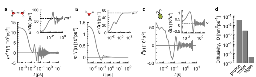
Figure 2: Friction at various spatial and temporal scales. (a) The memory kernel $\Gamma(t)$ and its running integral $G(t)=\int_{0}^{t}\Gamma(t^{\prime})dt^{\prime}$ for the proton-transfer dynamics presented in Figure 1a. The plateau value $G(t\rightarrow\infty)=\gamma$ evaluates the friction coefficient $\gamma$. $\Gamma(t)$, $G(t)$, and $\gamma$ (black dashed line) are scaled by $m^{-1}$ to facilitate comparison with non-equilibrium systems, which can be described using Eq. 2. (b) The friction on the center of mass of an individual water molecule in bulk liquid water (see Figure 1b). (c) The memory kernel $\bar{\Gamma}(t)$ and running integral $\bar{G}(t)=\int_{0}^{t}\bar{\Gamma}(t^{\prime})dt^{\prime}$ for a living and swimming Chlamydomonas reinhardtii algae cell (see Figure 1e). The plateau value $\bar{G}(t\rightarrow\infty)=\bar{\gamma}$ is used to evaluate the friction coefficient $\bar{\gamma}$. (d) The diffusivity $D=\langle\dot{x}^{2}\rangle\tau_{\text{m}}$ compared for the three systems, where $\tau_{\text{m}}=m\gamma^{-1}$ for the proton and the water molecule, and $\tau_{\text{m}}=\bar{\gamma}^{-1}$ for the algae cell. For equilibrium systems, where the equipartition theorem $\langle\dot{x}^{2}\rangle=k_{\text{B}}T/m$ holds (see Section 3.1), $D=k_{\text{B}}T/\gamma$.

In Figure 2a, we show $m^{-1}\Gamma(t)$ and $m^{-1}G(t)$ for the excess proton transport presented in Figure 1a. This system is characterized by length scales on the order of the OH water bond length, $1\;\textup{\AA}$, and time scales on the order of the vibrational period of the water OH bond, $10\;\text{fs}$. However, the memory friction along the reaction coordinate introduces additional time scales on the order of the structural relaxation time of the water environment, which is approximately $1\;\text{ps}$ [81]. The kernels exhibit both oscillating and decaying behavior, and we identify a plateau value of approximately $m^{-1}G(\infty)=m^{-1}\gamma=62\;\text{ps}^{-1}$, which can be used to evaluate the inertia time, $\tau_{\text{m}}=m/\gamma$, the timescale above which friction becomes relevant: $\tau_{\text{m}}=16\;\text{fs}$. The memory friction acting on the water molecule also exhibits a long-timescale decay (Figure 1b), on the order of $1$-$10\;\text{ps}$, with fewer oscillations than for the proton in Figure 2a, and is comparable to the relaxation timescale of water hydrogen bonding, which is approximately $8\;\text{ps}$. For the water molecule, we find $\tau_{\text{m}}=19\;\text{fs}$, similar to the value for the proton transfer reaction. However, the diffusivity, determined by the friction coefficient $\gamma$, is significantly different between these two systems due to their unequal masses. In Figure 1c, we show the friction acting on the Chlamydomonas reinhardtii algal cell, $\bar{\Gamma}(t)$ and $\bar{G}(t)$, where the cell dynamics are described using Eq. 2. The large and slowly decaying oscillations are associated with short-timescale flagella beating. For this cell, the extracted friction coefficient is $\bar{G}(\infty)=\bar{\gamma}=0.1{\times}10^{3}\;\text{s}^{-1}$. Therefore, we obtain $\tau_{\text{m}}=1/\bar{\gamma}=0.01\;\text{s}$. From the friction coefficient for each system, we compare the diffusivity $D=\langle\dot{x}^{2}\rangle\tau_{\text{m}}$ (Figure 2d), a suitable quantity for characterizing both equilibrium and non-equilibrium dynamics. In equilibrium, where temperature is defined and the equipartition theorem $\langle\dot{x}^{2}\rangle=k_{\text{B}}T/m$ holds, the diffusivity follows the familiar Einstein expression $D=k_{\text{B}}T/\gamma$. The diffusivity varies considerably between the three systems, spanning four orders of magnitude. As expected, cells, due to their large size, diffuse much more slowly than protons and water molecules.

5 Characteristic features of systems with non-Markovian friction

The study of molecular friction reveals characteristic signatures of non-Markovian friction effects on fundamental dynamic properties. In this section, we discuss key examples using simple model simulations, highlighting the generality of the implications for more complex systems.

5.1 Mean squared displacement

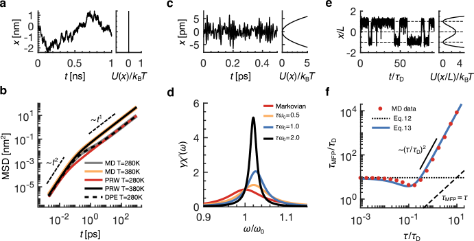
Figure 3: Memory effects on fundamental dynamic system properties. (a)-(b): The mean squared displacement (MSD) for a water molecule in bulk liquid water. (a) The time series for the oxygen atom $x$-component for a single water molecule from a molecular dynamics (MD) simulation of bulk water at $T=280\;\text{K}$. The molecule freely diffuses in the absence of a mean force potential. (b) MSDs are calculated from MD simulations at $T=280\;\text{K}$ (gray line) and $T=380\;\text{K}$ (yellow line). The persistent random walk model (PRW) describes the high-temperature MSD, capturing the ballistic ($\sim t^{2}$) and diffusive ($\sim t^{1}$) regimes (black line). However, it fails to capture the intermediate regime at low temperature (red line). This intermediate regime is described by the GLE with a memory kernel with a delta peak and a single exponential (delta-plus-exponential, DPE). (c)-(d): Velocity autocorrelation function spectral analysis for non-Markovian simulations. (c) The trajectory of a one-dimensional GLE simulation in a harmonic potential with strength $k=0.25k_{\text{B}}T/\text{pm}^{2}$ for a particle with mass $m=2\;\text{u}$ and a single-exponential memory kernel $\Gamma(t)=\gamma e^{-t/\tau}/\tau$ with $\tau\omega_{0}=10$. (d) Absorption spectra according to Eq. 10 from GLE simulations across various memory time scales, with $\tau_{\text{m}}\omega_{0}=10$ constant. The spectrum for a Markovian simulation $\tilde{\Gamma}(\omega)=\gamma$ is shown (solid red line). $\gamma\chi^{\prime\prime}(\omega_{0})=1$ for a single-exponential memory kernel, which follows from inserting the Fourier-transformed kernel $\tilde{\Gamma}(\omega)$ into Eq. 11. The systems with memory friction exhibit a blue shift and line narrowing. (e)-(f): Non-Markovian barrier-crossing kinetics. (e) The trajectory of a one-dimensional GLE simulation in a double-well potential $U(x)=U_{0}\big{[}(x/L)^{2}-1\big{]}^{2}$, with $U_{0}=3k_{\text{B}}T$ and characteristic length $L$. (f) Mean first-passage times (MFPT) $\tau_{\text{MFP}}$, measuring barrier-crossing times, are shown from GLE simulations (red points). Simulations are performed with a single-exponential memory kernel over a range of memory times $\tau$. The Markovian barrier crossing time prediction Eq. 12 is shown with the dotted black line and the non-Markovian prediction Eq. 13 is shown with the blue line. The black dashed line for $\tau_{\text{MFP}}=\tau_{\Gamma}$ indicates that reaction kinetics are influenced by non-Markovian effects even when $\tau\ll\tau_{\text{MFP}}$.

The mean squared displacement (MSD) is a fundamental measure in the study of diffusive molecular transport processes and statistical mechanics. As a time-correlation function, it measures the average distance a particle moves from its initial position over time, providing key insights into diffusion and molecular dynamics. The MSD can distinguish between different types of motion, such as Brownian or anomalous diffusion, and reveals how environmental factors like temperature or viscosity affect molecular dynamics.

[] Persistent random walk (PRW) modelA stochastic model for describing the motion of particles or organisms and includes the crossover from ballistic motion at short times to diffusive motion at long times. In Figure 3a, we show a typical trajectory for the $x$-component of a water molecule’s oxygen atom, taken from bulk liquid water simulations using classical force-field MD. In Figure 3b, we show the MSD for the motion of a single water molecule, simulated at two different temperatures. In a purely Markovian system with a delta-like memory kernel $\Gamma(t)=2\gamma\delta(t)$, one finds short-timescale ballistic dynamics with $\sim t^{2}$ scaling and long-timescale diffusive dynamics with $\sim t^{1}$ scaling. The MSD for a memoryless persistent random walk (PRW) is given by $\text{MSD}(t)=\langle(x(t)-x(0))^{2}\rangle=2D[t-\tau_{m}(1-e^{-t/\tau_{m}})]$, where $D$ is the diffusivity introduced in the previous section. The PRW accurately describes the MSD for water molecules at $T=380\;\text{K}$ but fails to describe the water MSD at $T=280\;\text{K}$. Recently, theoretical predictions were reported for MSDs that explicitly account for memory contributions suitable for systems with simple memory kernels that satisfy the general form $\bar{\Gamma}(t)=2a\delta(t)+be^{-t/\tau}\cos(\Omega t)$ [23]. In Figure 3b, we show that these non-Markovian predictions accurately describe the data for $T=280\;\text{K}$, using $\Gamma(t)$ parameters selected to optimize the agreement between the predicted MSD and the data ($\Omega=0$, $a=27.5\;\text{ps}$, $b=46.8\;\text{ps}^{-2}$, and $\tau=1.27\;\text{ps}$). The decrease of memory effects for higher temperatures highlights that memory contributions originate from water-water interactions, such as hydrogen bonds, which exert less influence as thermal fluctuations increase. Additionally, the effects of power-law memory kernel contributions [86, 87] or multi-exponential memory kernel contributions [88] on the MSD can be considered.

5.2 Velocity auto-correlation functions and vibrational spectra

[] Fluctuation-dissipation relation Exact relation between the two-point correlation function of an observable and the linear response of that observable to an external time-dependent force.

Vibrational spectroscopy is a powerful experimental tool for studying intra- and intermolecular interactions in liquids and solids. In linear absorption spectroscopy, the effective vibrational bond potential and frictional coupling between a vibrational mode and the environment are reflected in the line-shape of the absorption spectrum [81, 89, 90]. The linear absorption rate of a vibrational mode is proportional to the imaginary part of the frequency-dependent susceptibility $\tilde{\chi}^{\prime\prime}(\omega)$, which relates to the Fourier-transformed velocity autocorrelation function $C^{\dot{x}\dot{x}}(t)$ via the fluctuation-dissipation relation [91]

$$\omega\tilde{\chi}^{\prime\prime}(\omega)=\frac{\tilde{C}^{\dot{x}\dot{x}}(\omega)}{2k_{B}T}\,.$$ (10)

Vibrational spectroscopy covers a broad range of time scales, from collective modes and rotational motion in the GHz regime to rapid intramolecular vibrations in the high THz (i.e., the infrared) regime [12]. Conventionally, the line shape is interpreted by a combination of homogeneous and inhomogeneous line broadening effects, which characterize adiabatic energy dissipation and nonadiabatic coupling to the environment, respectively [89, 92, 90, 93]. In contrast, in the framework of the GLE, the coupling of a vibrational mode to the environment is described by the frequency-dependent friction function, which is the Fourier-transformed time-dependent memory friction kernel, which provides a timescale bridging approach to the theory of vibrational spectroscopy. Several studies have employed the GLE to model linear absorption and vibrational relaxation by modeling vibrational modes as anharmonic oscillators coupled to a thermal bath [9, 81, 94, 95, 96, 97, 98, 99]. Earlier works established the line-shifting and broadening principles of the GLE model but were limited by simple heuristic approximations for the friction function, which is obtained accurately using recent data-driven approaches [99, 81].

For a harmonic potential $U(x)=\frac{k}{2}x^{2}$, the linear response function $\tilde{\chi}(\omega)$, defined by the relation $\tilde{x}(\omega)=\tilde{\chi}(\omega)\tilde{F}_{R}(\omega)$ between force and position, is obtained by Fourier transformation of the GLE in Eq. 3 according to $\tilde{x}(\omega)=\int_{-\infty}^{\infty}dte^{\imath\omega t}x(t)$ as [81, 94, 95]

$$\tilde{\chi}(\omega)=\frac{1}{k-m\,\omega^{2}-i\omega\,\tilde{\Gamma}(\omega)}\,.$$ (11)

For Markovian friction $\tilde{\Gamma}(\omega)=\gamma$, the spectral peak of $\omega\tilde{\chi}^{\prime\prime}(\omega)$ is located at the eigenfrequency $\omega_{0}=\sqrt{k/m}$, with a peak value given by $\omega_{0}\tilde{\chi}^{\prime\prime}(\omega_{0})=1/\gamma$ and a full width at half maximum (FWHM) $\sigma=1/\tau_{\text{m}}$, where $\tau_{\text{m}}=m/\gamma$ is the inertia relaxation time, as discussed earlier. The time series trajectory in Figure 3c is generated using the Markovian embedding technique described in Section 3.3 for a particle with single-exponential memory $\Gamma(t)=\gamma e^{-t/\tau}/\tau$ in a harmonic potential, where $\tau$ is the memory time chosen as $\tau\omega_{0}=10$. In Figure 3d, we show spectra calculated using Eq. 10 for Markovian embedding simulations over a range of memory times for constant $\tau_{m}\omega_{0}=10$. The spectra exhibit a blue shift that is maximal for $\tau\omega_{0}=1$ and a continuous peak narrowing with increasing memory time $\tau$. These line shape changes, due to modifications of the velocity autocorrelation function, reflect non-Markovian effects [81].

5.3 Barrier-crossing reaction kinetics

In Figures 3e and 3f, we explore the consequences of memory effects on barrier-crossing reaction kinetics. For many systems, it is reasonable to assume the environment relaxes much faster than the barrier-crossing time scale. In these cases, one might be tempted to disregard memory effects entirely and use a theory assuming instantaneous friction, i.e., $\Gamma(t)=2\gamma\delta(t)$, such as the well-known Kramers’ theory [100], which is suitable across a wide range of dynamic regimes. Here, we show that this time scale argument does not hold. In the overdamped limit, where mass can be neglected and there is a position-dependent friction profile $\gamma(x)$, the mean first-passage (MFP) time to reach $x_{\text{b}}$ starting at $x_{\text{a}}$ follows from the Smoluchowski equation for Markovian diffusion in a free energy profile $U(x)$ as [] Kramers theoryThe first reaction rate theory to correctly account for the role of friction and inertia in predicting mean energy-barrier crossing times.

$$\tau_{\rm{MFP}}^{\rm{\text{Mar}}}=\frac{1}{k_{\rm{B}}T}\int\limits_{x_{\text{a}}}^{x_{\text{b}}}dx\gamma(x)\text{e}^{U(x)/k_{\rm{B}}T}\int\limits_{-\infty}^{x}dy\text{e}^{-U(y)/k_{\rm{B}}T}.$$ (12)

This formula is particularly useful for systems with low energy barriers, since the Kramers theory is known to be inaccurate in this limit. The limitations of different reaction rate theories in the presence of non-Markovian friction can be assessed by analysis of the GLE, as demonstrated for the prominent example of pair reaction dynamics in a solvent [43]. In Figure 3e, we show a typical trajectory from a Markovian embedding simulation (Section 3.3) with memory $\Gamma(t)=\gamma e^{-t/\tau}/\tau$. The external potential $U(x)=U_{0}\big{[}(x/L)^{2}-1\big{]}^{2}$ is a double-well with barrier height $U_{0}=3k_{\text{B}}T$. The simulations are performed in the overdamped limit ($\tau_{\text{m}}/\tau_{\text{D}}=0.001$) over a wide range of memory times, including the effective Markovian limit $\tau/\tau_{\text{D}}\rightarrow 0$. Reaction times are given as mean first-passage times $\tau_{\text{MFP}}$, evaluated from extended simulations [101, 102]. Here, $\tau_{\text{D}}=\gamma L^{2}/k_{\text{B}}T$ represents the diffusion time scale, i.e., the time taken for the particle to diffuse over a characteristic distance $L$ in the absence of a barrier. In the Markovian limit, $\tau_{\text{MFP}}$ approaches the exact Markovian prediction Eq. 12 for constant friction $\gamma(x)=\gamma$. As memory times are increased, the reaction times accelerate compared to the Markovian limit. This speed-up regime is predicted by the well-known Grote-Hynes theory [103] and was shown recently to be the dominant regime for many fast-folding proteins [51, 104]. However, for memory times beyond intermediate values $\tau>0.1\tau_{\text{D}}$, reaction times increase rapidly, following quadratic scaling $\tau_{\text{MFP}}\sim\tau^{2}$. The Grote-Hynes theory, which assumes time-scale separation between the relaxation of the environment and the barrier-crossing process, is known to break down for systems with long enough relaxation times [105, 101], and cannot predict the memory-induced slow-down regime. Later theories, such as Pollak, Grabert, and Hänggi theory, do capture this regime [106]. It is important to note that throughout both the reaction speed-up and slow-down regimes, the memory times are much smaller than barrier crossing times, dispelling the requirement that $\tau$ should be equal to, or larger than, $\tau_{\text{MFP}}$ in order to influence barrier crossing dynamics, which follows from a naive time-scale separation argument.

In recent years, we have seen the development of an alternative approach for predicting barrier-crossing times in systems with memory. The interpolating crossover formulas [101, 85, 107, 108] interpolate between the low friction and intermediate-to-high friction regimes of Kramers theory for arbitrary mass, including an empirical crossover term between the two limiting behaviors. Non-Markovian effects are introduced through effective friction and mass terms, derived from the two-point correlation of a non-Markovian system in a harmonic well. For a memory kernel of the form $\Gamma(t)=\gamma e^{-t/\tau}/\tau$, the equation becomes [85]

$$\begin{split}\frac{\tau_{\text{MFP}}}{\tau_{\text{D}}}=\frac{e^{U_{0}/k_{\text{B}}T}}{U_{0}/(k_{\text{B}}T)}\left[\left(\frac{\tau_{m}}{\tau_{\text{D}}}+\frac{4U_{0}}{k_{\text{B}}T}\frac{\tau^{2}}{\tau^{2}_{\text{D}}}\right)+\frac{\pi}{2\sqrt{2}}\frac{1}{1+10U_{0}\tau/(k_{\text{B}}T\tau_{\text{D}})}+2\sqrt{\frac{U_{0}\tau_{m}}{k_{\text{B}}T\tau_{\text{D}}}}\right],\end{split}$$ (13)

where the first term dominates under low friction, the second term under moderate to high friction, and the last term accounts for the turnover. This formula can extend to multi-exponential-component memory kernels [85, 107]. Figure 3 shows that Eq. 13 accurately models $\tau_{\text{MFP}}$ for the simulation parameters across all memory times.

6 Applications of GLE modeling and memory-kernel extraction

In this section, we detail three recent applications of GLE modeling and memory kernel extraction, spanning the nano-, micro-, and macroscale.

6.1 The nanoscale: molecular friction in protein folding

Molecular friction plays a central role in the study of protein folding [109]. It has been known for some time that protein folding times $\tau_{\rm{fold}}$ do not scale linearly with solvent viscosity $\eta$, which would be predicted from Kramers theory and from Eq. 12. This has led to the broad adoption of the notion of internal friction effects [65, 66, 67, 68, 69, 70, 71], where it is assumed that dissipative intramolecular interactions, unaffected by solvent viscosity, contribute significantly to the folding times. In general, the viscosity dependence of protein-folding times scale according to $\tau_{\rm{fold}}=\alpha\eta^{\beta}+\varepsilon$, where $\beta=1$ and $\varepsilon=0$ in the absence of internal friction and either $\beta<1$ or $\varepsilon>0$ when internal friction effects are present. Internal friction effects have been studied extensively with all-atom simulations, and various molecular origins have been proposed [110, 111, 112, 113, 36]; however, discussions have remained phenomenological without an explicit theory relating $\tau_{\rm{fold}}$ and $\eta$. Fundamentally, deviations from $\tau_{\rm{fold}}\sim\eta$ indicate deviations from either the Stokes-Einstein relationship or, for sufficiently overdamped systems, Kramers theory for activated barrier crossing processes $\tau_{\rm{fold}}\sim\gamma$, thus identifying friction as the key factor in internal friction effects. Without methods to directly evaluate friction, it has not been possible to test each of these relationships separately. Recently, memory kernel extraction techniques were applied directly to the rotation of selected torsion angles from small isomerizing molecules, demonstrating that deviations from $\tau_{\rm{fold}}\sim\eta$ must be ascribed to simultaneous violations of both the Stokes-Einstein relation and the overdamped Kramers relation [50]. Such a detailed analysis is still lacking for proteins.

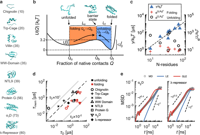
Figure 4: GLE analysis of all-atom protein folding simulations. (a) Native states of eight fast-folding proteins from extensive all-atom MD simulations [63]. (b) Free energy profile for the fraction of native contacts reaction coordinate $Q$ for the $\alpha_{3}$D protein. Configuration snapshots show example unfolded ($Q_{\rm{u}}$), barrier-top ($Q_{\rm{b}}$), and folded ($Q_{\rm{f}}$) states. The folding and unfolding reactions are shown. (c) The residue-number dependence of the friction coefficient $\gamma$ compared to the corresponding Arrhenius factor $\text{e}^{{U}_{0}/k_{\text{B}}T}$ for folding and unfolding transitions. Friction is divided by $k_{\rm{B}}T$ to account for unique system temperatures. A power law with an exponent $\sim 2.8$ (black-dashed line) shows a positive correlation between friction and protein chain length. (d) Memory-decay times $\tau_{\rm{mem}}$, calculated from the first moment of the memory kernel $\Gamma(t)$, compared to the diffusion times ($\tau_{\text{D}}=\gamma|Q_{\rm{b}}-Q_{\rm{u}}|^{2}/k_{\text{B}}T$ for folding and $\tau_{\text{D}}=\gamma|Q_{\rm{b}}-Q_{\rm{f}}|^{2}/k_{\text{B}}T$ for unfolding). Light gray lines indicate the bounding regime for $\tau_{\rm{mem}}$ between $\tau_{\rm{D}}{\times}10^{-2}$ and $\tau_{\rm{D}}{\times}10^{1}$, where memory-induced barrier-crossing acceleration is predicted. (e) Mean squared displacement (MSD) for the $\alpha_{3}$D and the $\lambda$-repressor proteins. All-atom MD simulation results are compared to a purely Markovian Langevin model (LE) and a non-Markovian GLE model. All results originally published in Dalton et al. [51]

.

To evaluate the friction experienced by a folding protein, one must first reduce the full atomic details of the protein and its solvating environment to a suitably chosen reaction coordinate. In all-atom simulations, one can explore reaction coordinates and pursue those that optimize statistical measures, such as the transition-path probability, evaluated via transition-path ensemble methods [114]. In the experimental context, one does not have the luxury of choosing optimal reaction coordinates, and a common choice is the inter-residue separation distance tracked indirectly by fluorescence resonance energy transfer (FRET) [15, 16, 17] or directly by single-molecule force spectroscopy (SMFS) [18, 19]. Regardless of technique, projecting onto a low-dimensional reaction coordinate is a coarse-graining procedure that incurs time-dependent, coordinate-specific friction. In protein folding, it is typically assumed that memory friction decays rapidly compared to relevant timescales, such as folding durations, leading to the conclusion that folding can be described by memoryless reaction-kinetic models. This enables the determination of friction via fitting procedures [115, 116]. As we demonstrated earlier (Section 5.3), this reasoning is not always justified. Still, Markovian techniques are commonly used to model protein folding [117, 118, 119, 120, 121]. However, recent investigations have shown that memory-dependent friction influences the long-timescale reaction kinetics of fast-folding proteins [51, 104] and $\alpha$-helix-forming polypeptide chains [42].

In Figure 4, we discuss a recent application of friction extraction techniques to extensive all-atom protein folding simulations. In Figure 4a, we show native states for eight fast-folding proteins selected from the seminal work by Lindorff-Larsen et al. [63]. Recently, memory-kernel extraction techniques were applied to these data, revealing the friction memory kernels associated with protein folding [51, 104]. In Figure 4b, we show the potential of mean force for the fraction of native contacts reaction coordinate $x=Q$ projected from the full atomic trajectory of the $\alpha_{3}$D fast-folding protein. The total simulation time for $\alpha_{3}$D is $707\;\mu\text{s}$, during which the protein completes 12 folding and unfolding events. Comparison of free energy landscapes for all eight proteins shows that barrier heights for folding and unfolding are not correlated with protein chain length (Figure 4c). The total friction acting on the reaction coordinate $\gamma$, however, is correlated, suggesting that friction likely plays an increasingly important role in determining protein folding times for larger proteins. Using the same fast-folding protein data set, $Q$ was previously argued to be the optimal reaction coordinate for capturing transition states [122], often considered an indication of minimal non-Markovian effects [123]. Despite this, the memory time scales in Figure 4d for the population of proteins in Figure 4a, estimated as the first moment of the memory kernel via $\tau_{\rm{mem}}=\int_{0}^{\infty}t\Gamma(t)dt/\int_{0}^{\infty}\Gamma(t)dt$, satisfy $1{\times}10^{-2}<\tau_{\text{mem}}/\tau_{\text{D}}<1{\times}10^{1}$, which is the regime in which memory effects are known to accelerate barrier-crossing reaction times [101]. Results show that the folding and unfolding times for these proteins are accelerated up to 10 times compared to Markovian predictions from Eq.12, and that the most accurate model for predicting protein folding and unfolding times is the multi-exponential extension of Eq.13, confirming that memory-dependent friction influences protein folding reaction kinetics.

Finally, when one analyzes the MSDs for this set of fast-folding proteins, one finds other hallmarks of memory friction effects. In Figure 4e, we show the MSDs from MD (grey circles) for the $\alpha_{3}$D and $\lambda$-repressor proteins. The plateau behavior at the longest timescale is due to the confinement of $Q$, which precludes long-time linear scaling, i.e., diffusive behavior. The intermediate regimes exhibit subdiffusive dynamics with exponents 0.4 and 0.5, characteristic of non-Markovian systems [87, 42]. Such subdiffusivity is often attributed to energy-landscape barriers. However, memoryless Langevin simulations performed on the extracted free energy profiles (blue lines) are diffusive for all time scales shorter than the confinement timescale. For multi-exponential Markovian embedding GLE simulations (see Section 3.3), parameterized by the memory kernels extracted for the $\alpha_{3}$D and $\lambda$-repressor proteins, the MSDs (red lines) agree well with the simulation results.

6.2 The microscale: classification of cell motion

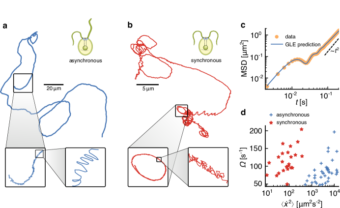
Figure 5: GLE-based cell motion classification scheme. (a) The swimming path of a Chlamydomonas reinhardtii algal cell with asynchronous flagella beating. The duration of the trajectory is $\sim 50\;\rm{s}$, and the magnification focuses on short time scales of the motion. The oscillatory cell motion due to flagella beating can be seen at the highest resolution. (b) A swimming path of a cell with synchronous flagella beating. The trajectory duration is also $\sim 50\;\rm{s}$. (c) The mean squared displacement for a single algal cell with asynchronous flagella beating (orange points) shows oscillating motion on 0.01 s to 0.1 s time scales. The cell’s directed motion shows a ballistic regime for time scales above 0.1 s. A theoretical prediction based on the GLE is also shown (blue line). (d) Cell-type classification based on the extracted GLE parameters. The oscillation frequency $\Omega$, evaluated by fitting $\bar{\Gamma}(t)=2a\delta(t)+be^{-t/\tau}\cos(\Omega t)$ (see Eq. 2) to the memory kernels of single cells, is plotted against the velocity variance $\langle\dot{x}^{2}\rangle$ for each cell. An unbiased cluster analysis reveals two distinct populations, corresponding to the swimming modes shown in (a) and (b). Results originally published in Klimek et al. [23]

Living organisms are active, non-equilibrium systems.

Therefore, for many processes in living systems, the equilibrium GLE models discussed so far may not suitably describe their dynamics. However, for studying long-time-scale motility and search dynamics, which are intrinsically stochastic processes, GLE models can indeed be applied [48, 23]. Various models have been proposed to describe the motion of different organisms [73, 74, 75]. Examples include using Lévy walks to model wandering albatross flights [78], and the run-and-tumble or active Ornstein-Uhlenbeck models to describe bacterial cell motion [124, 125]. Some of these models are special cases of the GLE [22, 126]. Why certain organisms exhibit specific dynamic patterns are unclear. However, in some cases, there is likely an evolutionary pressure to search efficiently for resources [76, 79]. Analyzing trajectories with the GLE reveals that different propulsion mechanisms lead to significantly different memory kernels. For example, human breast cancer cells show a negative memory component, leading to an extended ballistic regime in the MSD, while slime mold cells exhibit exponentially decaying memory [127]. Mouse fibroblasts and some other cells can be modeled by Markovian diffusion [128, 129].

In addition to modeling organism motion, the GLE, in combination with memory kernel extraction techniques, can be used as the basis for a scheme to classify cell motion. In Figure 5, we show swimming trajectories of two Chlamydomonas reinhardtii algal cells confined between glass plates, recorded using video microscopy. Analysis of the flagellar motion of individual cells reveals two distinct swimming modes [130]. The first mode, depicted in Figure 5a, is characterized by asynchronous flagella beating. This asynchronous beating leads to cell body wobbling, manifesting as short-time-scale oscillations observed in the finely magnified inset. The second distinct swimming mode is characterized by a synchronous breast-stroke motion of the flagella, as depicted in Figure 5b. On the shortest time scale, this synchronous beating leads to a back-and-forth motion. For both modes, the cells exhibit directed motion on intermediate time scales and diffusive behavior on long time scales. In Figure 5c, we show the MSD for a single asynchronously beating alga. The MSD resolves the oscillations from the flagella motion on 0.01 s to 0.1 s time scales, and above 0.1 s, the directed motion manifests as ballistic MSD ($\sim t^{2}$). The memory kernel, shown in Figure 2c, which has been extracted from the trajectory in Figure 5a, is well described by $\bar{\Gamma}(t)=2a\delta(t)+be^{-t/\tau}\cos(\Omega t)$ [23], which satisfies a general form that can be used to derive predictions for various two-point correlation functions, including the MSD and VACF. Such a prediction for the MSD, parameterized by fitting the memory kernel given in Figure 2c, agrees perfectly with the data in Figure 5c. Such a fitting scheme can be applied to parameterize the individual memory kernels evaluated for a population of cells. In Figure 5d, we show a scatter plot of the oscillation frequency $\Omega$ versus the mean-squared velocity $\langle\dot{x}^{2}\rangle$, collected over a population of single cells. The oscillation frequency $\Omega$ is positively correlated with the mean-squared velocity, indicating that faster flagella beating leads to faster swimming. Applying an unbiased cluster analysis to the complete space of extracted GLE model parameters reveals two distinct clusters that coincide with the groups of synchronously beating and asynchronously beating cell types. Since the friction kernel is sensitive to the short time scale dynamics of algal motion, the GLE can be used for single-cell parameter extraction, which can then be used for cell-type classification. Due to the generality of this data-driven GLE approach, there is great potential for application to many other kinds of organism motion or for classifying cell properties, such as elasticity or size.

6.3 The macroscale: predicting weather patterns

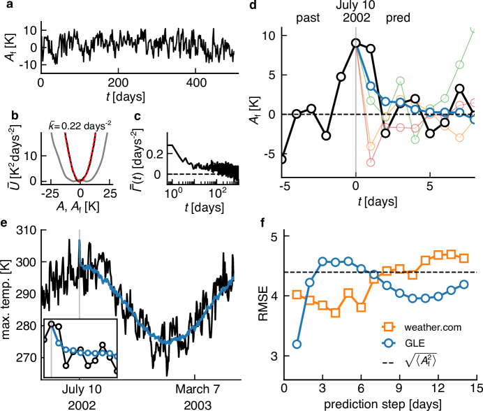
Figure 6: Predicting weather patterns using the GLE [131]. (a) The filtered temperature trajectory $A_{\text{f}}(t)$ obtained from the daily maximal temperature $A(t)$ in Figure 1f by removing the seasonal and slow components. (b) Effective potential $\bar{U}$ (see Eq. 2) of the unfiltered (gray) and filtered temperature data (black), compared with a harmonic potential $\bar{U}=\bar{k}A_{\text{f}}^{2}/2$ (dashed red). (c) Memory kernel, $\bar{\Gamma}(t)$, extracted from $A_{\text{f}}(t)$. (d) and (e) Illustration of the GLE prediction scheme applied to the maximal temperature in Berlin-Tegel. (d) The filtered temperature trajectory $A_{\text{f}}(t)$ over a 13-day period (black line). Thin colored lines show filtered trajectory predictions starting from July 10, 2002, using various random force realizations. The blue line shows the average over $N_{\text{p}}$ = 100 predictions. (e) Prediction of the maximal temperature $A(t)$ (blue), generated by adding seasonal and slow components to the predicted $A_{\text{f}}(t)$, shown against actual data (black). The inset shows the first eight prediction steps. (f) Comparison between the root-mean-squared error (RMSE) of a 14-day forecast, generated by the GLE model (blue), and predictions collected from the weather.com website (orange). The black-dashed line denotes the standard deviation of $A_{\text{f}}(t)$, serving as a prediction benchmark.

The need to make sense of time-series data has implications across all spatial scales, from nanoscale to terrestrial scales. In meteorology and climatology, traditional models rely on basic physical principles such as conservation laws [132]. In recent years, univariate and multivariate stochastic models [133, 134] and machine-learning (ML) methods have been developed and applied to the study of weather patterns [135, 136, 137, 138, 139, 140]. Despite being universally applicable to such diverse data types, ML techniques also face considerable criticism. First, determining the exorbitant number of parameters necessary for accurate modeling incurs high computational costs for model training [141, 142]. Second, ML is often viewed as a black box, and the lack of interpretability of the learned rules is often unsatisfactory for applications in the natural sciences. The GLE is a general stochastic model and has been applied to financial and meteorological data [143, 144] and has been used to predict stochastic time-series data [38]. In time series analysis, the data are often decomposed into long-term trends, such as seasonal modes, and the remaining short-term components, which are often neglected or treated as stochastic [136, 145]. This ad hoc decomposition makes the equation governing the dynamics of the remaining short-term components ill-defined. Here, we treat the raw signal $x(t)=A(t)$ using convolution filtering [131] according to

$$A_{\text{f}}(t)=\int_{-\infty}^{\infty}dt^{\prime}A(t-t^{\prime})f(t^{\prime}).$$ (14)

By constructing a filter function $f(t)$ that is a combination of low- and band-pass filters, the observable $A(t)$ can be exactly decomposed as $A(t)=A_{\text{f}}(t)+A_{\text{lp}}(t)+A_{\text{bp}}(t)$, where $A_{\text{f}}(t)$ is the fast-filtered component, $A_{\text{lp}}(t)$ is the slow, low-pass-filtered trend, and $A_{\text{bp}}(t)$ is the periodic, band-pass-filtered component. The slow and oscillating components $A_{\text{lp}}(t)$ and $A_{\text{bp}}(t)$ can be treated with deterministic models or fitted, the fast-filtered component $A_{\text{f}}(t)$ in fact, can be modeled by a GLE of the form given in Eq. 2 [146]. The memory kernel $\bar{\Gamma}(t)$ can be extracted from the filtered time series $A_{\text{f}}(t)$ using previously discussed methods to predict the future trajectory $A(t)$.

The daily maximal temperature trajectory $A(t)$ for Berlin-Tegel in Figure 1f exhibits pronounced seasonal variation typical for a continental European climate, as seen from the filtered complement $A(t)-A_{\text{f}}(t)$, shown by the red line in Figure 1f. The filtered signal $A_{\text{f}}(t)$, shown in Figure 6a, exhibits stochastic behavior with temperature fluctuations in the range of $\pm$10 K. The effective potential for $A(t)$, given by $\bar{U}(A)=-\langle\dot{A}^{2}\rangle\log\rho(A)$, is shown in Figure 6b as a gray line. The two minima, reflecting the mean winter and summer temperatures, indicate that $A(t)$ is significantly non-Gaussian. The effective potential for the filtered trajectory $A_{\text{f}}(t)$ is harmonic (black line in Figure 6b), given by $\bar{U}(A_{\text{f}})=\bar{k}A_{\text{f}}^{2}/2$, with $\bar{k}=\langle\dot{A}_{\text{f}}^{2}\rangle/\langle A_{\text{f}}^{2}\rangle=0.22$ days^-2. This indicates that $A_{\text{f}}(t)$ is an effectively Gaussian stochastic variable. Therefore, the GLE in Eq. 2 is a suitable model for $A_{\text{f}}(t)$ [48, 23]. The memory kernel $\bar{\Gamma}(t)$, extracted from $A_{\text{f}}(t)$ (shown in Figure 6c), decays over many days, clearly revealing the non-Markovian nature of the daily temperature variation. To illustrate the GLE’s predictive application, we arbitrarily set July 10, 2002, as the prediction date. To illustrate the process, we generate 100 realizations of the discrete future random force $\bar{F}_{\text{R}}$, which is conditioned on the history of $\bar{F}_{\text{R}}$, obtained by inversion of the GLE [28]. In Figure 6d, three representative instances of the stochastic predictions of $A_{\text{f}}$ are shown. These predictions exhibit fluctuations similar to the actual filtered signal. The mean prediction, averaged over all instances, decays after a few days. After adding the filter complement $A(t)-A_{\text{f}}(t)$, we compare the full prediction of $A(t)$ from July 10, 2002 on with the actual temperature in Figure 6e. We quantify the accuracy of the prediction using the root-mean-squared error, $\text{RMSE}(j\Delta t)=\sqrt{\sum_{i=1}^{N_{\text{s}}}\bigl{[}A(t_{i}+j\Delta t)-{A}_{\text{pred}}(t_{i}+j\Delta t)\big{]}^{2}/N_{\text{s}}}$, for $N_{\text{s}}=60$ predictions with randomly selected start times between March 9, 2020, and May 25, 2020. ${A}(t_{i}+j\Delta t)$ denotes the actual temperature trajectory, while ${A}_{\text{pred}}(t_{i}+j\Delta t)$ denotes the prediction starting at time $t_{i}$, with $i=1,2,\dots,N_{\text{s}}$. In Figure 6f, the GLE forecasts are more accurate than commercial weather.com forecasts for single-day predictions and perform comparably overall. Additionally, GLE prediction methods are also much faster than state-of-the-art machine-learning techniques. This demonstrates the potential usefulness of predictions of complex data with the GLE.

[SUMMARY POINTS]

1. We describe how the GLE can be used to analyze equilibrium and non-equilibrium time-series data from different disciplines. We discuss methods to derive GLEs, extract GLE parameters from time-series data, and simulate the GLE.

2. For general model systems, we show that memory effects significantly modify diffusional behavior (described by MSD), vibrational behavior (described by the velocity-autocorrelation function), and barrier-crossing time in a bistable potential.

3. The usefulness of the GLE approach is demonstrated with examples such as protein-folding dynamics, motility patterns of single cells, and weather data analysis and prediction.

[FUTURE ISSUES]

1. Robust methods for extracting GLE parameters from noisy and time-discretized experimental data need improvement [37].

2. The derivation of GLEs that include non-linear friction effects and can be simulated by efficient embedding techniques presents an open issue [29, 80].

3. The accurate prediction of non-Markovian reaction kinetics in arbitrary free energy landscapes is relevant for protein folding and chemical reaction kinetics but is not possible with current analytical reaction rate theories.

4. The derivation and characterization of GLEs applicable to systems that are far from equilibrium even in their stationary state is an active research field [41, 48, 47]. Methods to detect and characterize non-equilibrium properties of systems based on time series data are particularly needed [147].

DISCLOSURE STATEMENT

The authors are not aware of any affiliations, memberships, funding, or financial holdings that might be perceived as affecting the objectivity of this review.

References

- [1] Zwanzig R, Bixon M. 1970. Hydrodynamic Theory of the Velocity Correlation Function. Physical Review A 2(5):2005–2012
- [2] Español P, Zúñiga I. 1993. Force autocorrelation function in Brownian motion theory. The Journal of Chemical Physics 98(1):574–580
- [3] Bocquet L, Piasecki J, Hansen JP. 1994. On the Brownian motion of a massive sphere suspended in a hard-sphere fluid. I. Multiple-time-scale analysis and microscopic expression for the friction coefficient. Journal of Statistical Physics 76(1):505–526
- [4] Mason TG, Weitz DA. 1995. Optical Measurements of Frequency-Dependent Linear Viscoelastic Moduli of Complex Fluids. Physical Review Letters 74(7):1250–1253
- [5] Crocker JC, Valentine MT, Weeks ER, Gisler T, Kaplan PD, et al. 2000. Two-Point Microrheology of Inhomogeneous Soft Materials. Physical Review Letters 85(4):888–891
- [6] Lesnicki D, Vuilleumier R, Carof A, Rotenberg B. 2016. Molecular Hydrodynamics from Memory Kernels. Physical Review Letters 116(14):147804
- [7] Straub JE, Borkovec M, Berne BJ. 1987. Calculation of dynamic friction on intramolecular degrees of freedom. The Journal of Physical Chemistry 91(19):4995–4998
- [8] Berne BJ, Tuckerman ME, Straub JE, Bug ALR. 1990. Dynamic friction on rigid and flexible bonds. The Journal of Chemical Physics 93(7):5084–5095
- [9] Tuckerman M, Berne BJ. 1993. Vibrational relaxation in simple fluids: Comparison of theory and simulation. The Journal of Chemical Physics 98(9):7301–7318
- [10] Heyden M, Sun J, Funkner S, Mathias G, Forbert H, et al. 2010. Dissecting the THz spectrum of liquid water from first principles via correlations in time and space. Proceedings of the National Academy of Sciences 107(27):12068–12073
- [11] Lesnicki D, Sulpizi M. 2018. A Microscopic Interpretation of Pump-Probe Vibrational Spectroscopy Using Ab Initio Molecular Dynamics. J. Phys. Chem. B 122(25):6604–6609
- [12] Carlson S, Brünig FN, Loche P, Bonthuis DJ, Netz RR. 2020. Exploring the Absorption Spectrum of Simulated Water from MHz to Infrared. J. Phys. Chem. A 124(27):5599–5605
- [13] Furst EM, Squires TM. 2017. Microrheology. Oxford University Press
- [14] Schmidt RF, Kiefer H, Dalgliesh R, Gradzielski M, Netz RR. 2024. Nanoscopic Interfacial Hydrogel Viscoelasticity Revealed from Comparison of Macroscopic and Microscopic Rheology. Nano Letters 24(16):4758–4765
- [15] Schuler B, Eaton WA. 2008. Protein folding studied by single-molecule FRET. Current Opinion in Structural Biology 18(1):16–26
- [16] Chung HS, McHale K, Louis JM, Eaton WA. 2012. Single-Molecule Fluorescence Experiments Determine Protein Folding Transition Path Times. Science 335(6071):981–984
- [17] Chung HS, Eaton WA. 2013. Single-molecule fluorescence probes dynamics of barrier crossing. Nature 502(7473):685–688
- [18] Neupane K, Foster DAN, Dee DR, Yu H, Wang F, Woodside MT. 2016. Direct observation of transition paths during the folding of proteins and nucleic acids. Science 352(6282):239–242
- [19] Neupane K, Manuel AP, Woodside MT. 2016. Protein folding trajectories can be described quantitatively by one-dimensional diffusion over measured energy landscapes. Nature Physics 12(7):700–703
- [20] Ridley AJ, Schwartz MA, Burridge K, Firtel RA, Ginsberg MH, et al. 2003. Cell Migration: Integrating Signals from Front to Back. Science 302(5651):1704–1709
- [21] Maiuri P, Terriac E, Paul-Gilloteaux P, Vignaud T, McNally K, et al. 2012. The first World Cell Race. Current Biology 22(17):R673–R675
- [22] Mitterwallner BG, Schreiber C, Daldrop JO, Rädler JO, Netz RR. 2020. Non-Markovian data-driven modeling of single-cell motility. Physical Review E 101(3):32408
- [23] Klimek A, Mondal D, Block S, Sharma P, Netz RR. 2024. Data-driven classification of individual cells by their non-Markovian motion. Biophysical Journal 123(10):1173–1183
- [24] Nakajima S. 1958. On Quantum Theory of Transport Phenomena: Steady Diffusion. Progress of Theoretical Physics 20(6):948–959
- [25] Mori H. 1965a. Transport, Collective Motion, and Brownian Motion. Progress of Theoretical Physics 33(3):423–455
- [26] Mori H. 1965b. A Continued-Fraction Representation of the Time-Correlation Functions. Progress of Theoretical Physics 34(3):399–416
- [27] Zwanzig R. 1961. Memory Effects in Irreversible Thermodynamics. Physical Review 124(4):983–992
- [28] Carof A, Vuilleumier R, Rotenberg B. 2014. Two Algorithms to Compute Projected Correlation Functions in Molecular Dynamics Simulations. The Journal of Chemical Physics 140(12):124103
- [29] Ayaz C, Scalfi L, Dalton BA, Netz RR. 2022. Generalized Langevin equation with a nonlinear potential of mean force and nonlinear memory friction from a hybrid projection scheme. Physical Review E 105(5):54138
- [30] Vroylandt H. 2022. On the derivation of the generalized Langevin equation and the fluctuation-dissipation theorem. Europhysics Letters 140(6):62003
- [31] Vroylandt H, Monmarché P. 2022. Position-dependent memory kernel in generalized Langevin equations: Theory and numerical estimation. The Journal of Chemical Physics 156(24):244105
- [32] Vroylandt H, Goudenège L, Monmarché P, Pietrucci F, Rotenberg B. 2022. Likelihood-based non-Markovian models from molecular dynamics. Proceedings of the National Academy of Sciences 119(13):e2117586119
- [33] Berne BJ, Harp GD. 1970. On the Calculation of Time Correlation Functions. Advances in Chemical Physics 17:63–227
- [34] Lange OF, Grubmüller H. 2006. Collective Langevin dynamics of conformational motions in proteins. The Journal of Chemical Physics 124(21):214903
- [35] Jung G, Hanke M, Schmid F. 2017. Iterative Reconstruction of Memory Kernels. J. Chem. Theory Comput. 13(6):2481–2488
- [36] Daldrop JO, Kappler J, Brünig FN, Netz RR. 2018. Butane dihedral angle dynamics in water is dominated by internal friction. Proceedings of the National Academy of Sciences 115(20):5169–5174
- [37] Tepper L, Dalton B, Netz RR. 2024. Accurate Memory Kernel Extraction from Discretized Time-Series Data. Journal of Chemical Theory and Computation 20(8):3061–3068
- [38] Chorin AJ, Hald OH, Kupferman R. 2000. Optimal Prediction and the Mori-Zwanzig Representation of Irreversible Processes. Proceedings of the National Academy of Sciences 97(7):2968–2973
- [39] Darve E, Solomon J, Kia A. 2009. Computing generalized Langevin equations and generalized Fokker–Planck equations. Proceedings of the National Academy of Sciences 106(27):10884–10889
- [40] Straube AV, Kowalik BG, Netz RR, Höfling F. 2020. Rapid onset of molecular friction in liquids bridging between the atomistic and hydrodynamic pictures. Communications Physics 3(1):126
- [41] Schilling T. 2022. Coarse-grained modelling out of equilibrium. Physics Reports 972:1–45
- [42] Ayaz C, Tepper L, Brünig FN, Kappler J, Daldrop JO, Netz RR. 2021. Non-Markovian modeling of protein folding. Proceedings of the National Academy of Sciences 118(31):e2023856118
- [43] Brünig FN, Daldrop JO, Netz RR. 2022. Pair-Reaction Dynamics in Water: Competition of Memory, Potential Shape, and Inertial Effects. The Journal of Physical Chemistry B 126(49):10295–10304
- [44] Lau AWC, Hoffman BD, Davies A, Crocker JC, Lubensky TC. 2003. Microrheology, stress fluctuations, and active behavior of living cells. Physical Review Letters 91(19):198101
- [45] Gnesotto FS, Mura F, Gladrow J, Broedersz CP. 2018. Broken detailed balance and non-equilibrium dynamics in living systems: a review. Reports on Progress in Physics 81(6):66601
- [46] Abbasi A, Netz RR, Naji A. 2023. Non-Markovian Modeling of Nonequilibrium Fluctuations and Dissipation in Active Viscoelastic Biomatter. Physical Review Letters 131(22):228202
- [47] Meyer H, Wolf S, Stock G, Schilling T. 2021. A Numerical Procedure to Evaluate Memory Effects in Non-Equilibrium Coarse-Grained Models. Advanced Theory and Simulations 4(4):2000197
- [48] Netz RR. 2024a. Derivation of the nonequilibrium generalized Langevin equation from a time-dependent many-body Hamiltonian. Physical Review E 110(1):14123
- [49] Brünig FN, Hillmann P, Kim WK, Daldrop JO, Netz RR. 2022a. Proton-transfer spectroscopy beyond the normal-mode scenario. The Journal of Chemical Physics 157(17):174116
- [50] Dalton BA, Kiefer H, Netz RR. 2024. The role of memory-dependent friction and solvent viscosity in isomerization kinetics in viscogenic media. Nature Communications 15(1):3761
- [51] Dalton BA, Ayaz C, Kiefer H, Klimek A, Tepper L, Netz RR. 2023. Fast protein folding is governed by memory-dependent friction. Proceedings of the National Academy of Sciences 120(31):e2220068120
- [52] Wraight CA. 2006. Chance and Design-Proton Transfer in Water, Channels and Bioenergetic Proteins. Biochim. Biophys. Acta BBA - Bioenerg. 1757(8):886–912
- [53] Agmon N, Bakker HJ, Campen RK, Henchman RH, Pohl P, et al. 2016. Protons and Hydroxide Ions in Aqueous Systems. Chem. Rev. 116(13):7642–7672
- [54] Agmon N. 1995. The Grotthuss Mechanism. Chem. Phys. Lett. 244(5-6):456–462
- [55] Marx D. 2006. Proton Transfer 200 Years after Von Grotthuss: Insights from Ab Initio Simulations. ChemPhysChem 7(9):1848–1870
- [56] Thämer M, De Marco L, Ramasesha K, Mandal A, Tokmakoff A. 2015. Ultrafast 2D IR Spectroscopy of the Excess Proton in Liquid Water. Science 350(6256):78–82
- [57] Dahms F, Fingerhut BP, Nibbering ETJ, Pines E, Elsaesser T. 2017. Large-Amplitude Transfer Motion of Hydrated Excess Protons Mapped by Ultrafast 2D IR Spectroscopy. Science 357(6350):491–495
- [58] Roy S, Schenter GK, Napoli JA, Baer MD, Markland TE, Mundy CJ. 2020. Resolving Heterogeneous Dynamics of Excess Protons in Aqueous Solution with Rate Theory. J. Phys. Chem. B 124(27):5665–5675
- [59] Brünig FN, Rammler M, Adams EM, Havenith M, Netz RR. 2022b. Spectral signatures of excess-proton waiting and transfer-path dynamics in aqueous hydrochloric acid solutions. Nature Communications 13(1):4210
- [60] Kowalik B, Daldrop JO, Kappler J, Schulz JCF, Schlaich A, Netz RR. 2019. Memory-kernel extraction for different molecular solutes in solvents of varying viscosity in confinement. Physical Review E 100(1):012126
- [61] Scalfi L, Vitali D, Kiefer H, Netz RR. 2023. Frequency-dependent hydrodynamic finite size correction in molecular simulations reveals the long-time hydrodynamic tail. The Journal of Chemical Physics 158(19):191101
- [62] Yamaguchi T. 2021. Molecular dynamics simulation study on the isomerization reaction in a solvent with slow structural relaxation. Chemical Physics 542:111056
- [63] Lindorff-Larsen K, Piana S, Dror RO, Shaw DE. 2011. How Fast-Folding Proteins Fold. Science 334(6055):517 LP – 520
- [64] Shaw DE, Dror RO, Salmon JK, Grossman JP, Mackenzie KM, et al. 2009. Millisecond-scale molecular dynamics simulations on Anton. In Proceedings of the Conference on High Performance Computing Networking, Storage and Analysis, pp. 1–11
- [65] Beece D, Eisenstein L, Frauenfelder H, Good D, Marden MC, et al. 1980. Solvent viscosity and protein dynamics. Biochemistry 19(23):5147–5157
- [66] Doster W. 1983. Viscosity scaling and protein dynamics. Biophysical chemistry 17(2):97–103
- [67] Ansari A, Jones CM, Henry ER, Hofrichter J, Eaton WA. 1992. The role of solvent viscosity in the dynamics of protein conformational changes. Science 256(5065):1796 LP – 1798
- [68] Jas GS, Eaton WA, Hofrichter J. 2001. Effect of Viscosity on the Kinetics of -Helix and -Hairpin Formation. The Journal of Physical Chemistry B 105(1):261–272
- [69] Hagen SJ. 2010. Solvent viscosity and friction in protein folding dynamics. Current protein & peptide science 11(5):385–395
- [70] Soranno A, Buchli B, Nettels D, Cheng RR, Müller-Späth S, et al. 2012. Quantifying internal friction in unfolded and intrinsically disordered proteins with single-molecule spectroscopy. Proceedings of the National Academy of Sciences 109(44):17800 LP–17806
- [71] Borgia A, Wensley BG, Soranno A, Nettels D, Borgia MB, et al. 2012. Localizing internal friction along the reaction coordinate of protein folding by combining ensemble and single-molecule fluorescence spectroscopy. Nature Communications 3(1):1195
- [72] Klafter J, Sokolov IM. 2005. Anomalous diffusion spreads its wings. Physics World 18(8):29
- [73] Bartumeus F, da Luz MGE, Viswanathan GM, Catalan J. 2005. Animal search strategies: a quantitative random-walk analysis. Ecology 86(11):3078–3087
- [74] Johnson DS, London JM, Lea MA, Durban JW. 2008. Continuous-time correlated random walk model for animal telemetry data. Ecology 89(5):1208–1215
- [75] Dieterich P, Klages R, Preuss R, Schwab A. 2008. Anomalous dynamics of cell migration. Proceedings of the National Academy of Sciences 105(2):459–463
- [76] Viswanathan GM, Da Luz MGE, Raposo EP, Stanley HE. 2011. The physics of foraging: an introduction to random searches and biological encounters. Cambridge University Press
- [77] Viswanathan GM, Afanasyev V, Buldyrev SV, Murphy EJ, Prince PA, Stanley HE. 1996. Lévy flight search patterns of wandering albatrosses. Nature 381(6581):413–415
- [78] Edwards AM, Phillips RA, Watkins NW, Freeman MP, Murphy EJ, et al. 2007. Revisiting Lévy flight search patterns of wandering albatrosses, bumblebees and deer. Nature 449(7165):1044–1048
- [79] Klimek A, Netz RR. 2022. Optimal non-Markovian composite search algorithms for spatially correlated targets. Europhysics Letters 139(3):32003
- [80] Ayaz C, Tepper L, Netz RR. 2022. Self-consistent Markovian embedding of generalized Langevin equations with configuration-dependent mass and a nonlinear friction kernel. Turkish Journal of Physics 46(6):194
- [81] Brünig FN, Geburtig O, von Canal A, Kappler J, Netz RR. 2022c. Time-Dependent Friction Effects on Vibrational Infrared Frequencies and Line Shapes of Liquid Water. The Journal of Physical Chemistry B 126(7):1579–1589
- [82] Risken H. 1996. The Fokker-Planck Equation: Methods of Solution and Applications. Berlin, Heidelberg: Springer Berlin Heidelberg
- [83] Ceriotti M, Bussi G, Parrinello M. 2010. Colored-Noise Thermostats à la Carte. Journal of Chemical Theory and Computation 6(4):1170–1180
- [84] Zwanzig R. 1973. Nonlinear Generalized Langevin Equations. J Stat Phys 9(3):215–220
- [85] Kappler J, Hinrichsen VB, Netz RR. 2019. Non-Markovian barrier crossing with two-time-scale memory is dominated by the faster memory component. The European Physical Journal E 42(9):119
- [86] Kou SC, Xie XS. 2004. Generalized Langevin equation with fractional Gaussian noise: subdiffusion within a single protein molecule. Physical Review Letters 93:180603–180800
- [87] Goychuk I. 2009. Viscoelastic subdiffusion: From anomalous to normal. Physical Review E 80(4):46125
- [88] Goychuk I. 2012. Viscoelastic subdiffusion: generalized Langevin equation approach. Advances in Chemical Physics 150:187–253
- [89] Schrader B, ed. 1995. Infrared and Raman Spectroscopy: Methods and Applications. New York: Wiley-VCH
- [90] Bakker HJ, Skinner JL. 2010. Vibrational Spectroscopy as a Probe of Structure and Dynamics in Liquid Water. Chem. Rev. 110(3):1498–1517
- [91] Kubo R. 1966. The Fluctuation-Dissipation Theorem. Rep. Prog. Phys. 29(1):306
- [92] Auer BM, Skinner JL. 2008. IR and Raman Spectra of Liquid Water: Theory and Interpretation. J. Chem. Phys. 128(22):224511
- [93] Perakis F, De Marco L, Shalit A, Tang F, Kann ZR, et al. 2016. Vibrational Spectroscopy and Dynamics of Water. Chem. Rev. 116(13):7590–7607
- [94] Metiu H, Oxtoby DW, Freed KF. 1977. Hydrodynamic Theory for Vibrational Relaxation in Liquids. Phys. Rev. A 15(1):361–371
- [95] Oxtoby DW. 1981. Vibrational Relaxation in Liquids. Annual Review of Physical Chemistry 32:77–101
- [96] Adelman SA, Stote RH. 1988. Theory of Vibrational Energy Relaxation in Liquids: Construction of the Generalized Langevin Equation for Solute Vibrational Dynamics in Monatomic Solvents. J. Chem. Phys. 88(7):4397–4414
- [97] Smith DE, Harris CB. 1990. Generalized Brownian Dynamics. II. Vibrational Relaxation of Diatomic Molecules in Solution. J. Chem. Phys. 92(2):1312–1319
- [98] Bader JS, Berne BJ, Pollak E, Hänggi P. 1996. The Energy Relaxation of a Nonlinear Oscillator Coupled to a Linear Bath. J. Chem. Phys. 104(3):1111–1119
- [99] Gottwald F, Ivanov SD, Kühn O. 2016. Vibrational Spectroscopy via the Caldeira-Leggett Model with Anharmonic System Potentials. J. Chem. Phys. 144(16)
- [100] Kramers HA. 1940. Brownian motion in a field of force and the diffusion model of chemical reactions. Physica 7(4):284–304
- [101] Kappler J, Daldrop JO, Brünig FN, Boehle MD, Netz RR. 2018. Memory-induced acceleration and slowdown of barrier crossing. The Journal of Chemical Physics 148(1):14903
- [102] Zhou Q, Netz RR, Dalton BA. 2024. Rapid state-recrossing kinetics in non-Markovian systems. arXiv:2403.06604 [cond-mat.stat-mech]
- [103] Grote RF, Hynes JT. 1980. The stable states picture of chemical reactions. II. Rate constants for condensed and gas phase reaction models. The Journal of Chemical Physics 73(6):2715–2732
- [104] Dalton BA, Netz RR. 2024. pH Modulates Friction Memory Effects in Protein Folding. Physical Review Letters 133(18):188401
- [105] Straub JE, Borkovec M, Berne BJ. 1986. Non‐Markovian activated rate processes: Comparison of current theories with numerical simulation data. The Journal of Chemical Physics 84(3):1788–1794
- [106] Pollak E, Grabert H, Hänggi P. 1989. Theory of activated rate processes for arbitrary frequency dependent friction: Solution of the turnover problem. The Journal of Chemical Physics 91(7):4073–4087
- [107] Lavacchi L, Kappler J, Netz RR. 2020. Barrier crossing in the presence of multi-exponential memory functions with unequal friction amplitudes and memory times. EPL 131(4)
- [108] Lavacchi L, Daldrop JO, Netz RR. 2022. Non-Arrhenius barrier crossing dynamics of non-equilibrium non-Markovian systems. Europhysics Letters 139(5):51001
- [109] Plotkin SS, Wolynes PG. 1998. Non-Markovian Configurational Diffusion and Reaction Coordinates for Protein Folding. Physical Review Letters 80(22):5015–5018
- [110] Schulz JCF, Schmidt L, Best RB, Dzubiella J, Netz RR. 2012. Peptide Chain Dynamics in Light and Heavy Water: Zooming in on Internal Friction. Journal of the American Chemical Society 134(14):6273–6279
- [111] Echeverria I, Makarov DE, Papoian GA. 2014. Concerted Dihedral Rotations Give Rise to Internal Friction in Unfolded Proteins. Journal of the American Chemical Society 136(24):8708–8713
- [112] de Sancho D, Sirur A, Best RB. 2014. Molecular origins of internal friction effects on protein-folding rates. Nature Communications 5:4307
- [113] Zheng W, De Sancho D, Hoppe T, Best RB. 2015. Dependence of Internal Friction on Folding Mechanism. Journal of the American Chemical Society 137(9):3283–3290
- [114] Best RB, Hummer G. 2005. Reaction coordinates and rates from transition paths. Proceedings of the National Academy of Sciences 102(19):6732 LP–6737
- [115] Hummer G. 2005. Position-dependent diffusion coefficients and free energies from Bayesian analysis of equilibrium and replica molecular dynamics simulations. New Journal of Physics 7(1):34
- [116] Gopich IV, Szabo A. 2009. Decoding the Pattern of Photon Colors in Single-Molecule FRET. The Journal of Physical Chemistry B 113(31):10965–10973
- [117] Muñoz V, Eaton WA. 1999. A simple model for calculating the kinetics of protein folding from three-dimensional structures. Proceedings of the National Academy of Sciences 96(20):11311–11316
- [118] Best RB, Hummer G. 2006. Diffusive model of protein folding dynamics with Kramers turnover in rate. Physical Review Letters 96(22):228104
- [119] Best RB, Hummer G. 2010. Coordinate-dependent diffusion in protein folding. Proceedings of the National Academy of Sciences 107(3):1088 LP–1093
- [120] Zheng W, Best RB. 2015. Reduction of All-Atom Protein Folding Dynamics to One-Dimensional Diffusion. The Journal of Physical Chemistry B 119(49):15247–15255
- [121] Chung HS, Piana-Agostinetti S, Shaw DE, Eaton WA. 2015. Structural origin of slow diffusion in protein folding. Science (New York, N.Y.) 349(6255):1504–1510
- [122] Best RB, Hummer G, Eaton WA. 2013. Native contacts determine protein folding mechanisms in atomistic simulations. Proceedings of the National Academy of Sciences 110(44):17874 LP–17879
- [123] Berezhkovskii AM, Makarov DE. 2018. Single-Molecule Test for Markovianity of the Dynamics along a Reaction Coordinate. The Journal of Physical Chemistry Letters 9(9):2190–2195
- [124] Tailleur J, Cates ME. 2008. Statistical mechanics of interacting run-and-tumble bacteria. Physical review letters 100(21):218103
- [125] Martin D, O’Byrne J, Cates ME, Fodor É, Nardini C, et al. 2021. Statistical mechanics of active Ornstein-Uhlenbeck particles. Physical Review E 103(3):32607
- [126] Mitterwallner BG, Lavacchi L, Netz RR. 2020. Negative friction memory induces persistent motion. The European Physical Journal E 43:1–11
- [127] Li L, Cox EC, Flyvbjerg H. 2011. ‘Dicty dynamics’: Dictyostelium motility as persistent random motion. Physical biology 8(4):46006
- [128] Gail MH, Boone CW. 1970. The locomotion of mouse fibroblasts in tissue culture. Biophysical journal 10(10):980–993
- [129] Wright A, Li YH, Zhu C. 2008. The differential effect of endothelial cell factors on in vitro motility of malignant and non-malignant cells. Annals of biomedical engineering 36:958–969
- [130] Mondal D, Prabhune AG, Ramaswamy S, Sharma P. 2021. Strong confinement of active microalgae leads to inversion of vortex flow and enhanced mixing. Elife 10:e67663
- [131] Kiefer H, Furtel D, Ayaz C, Klimek A, Daldrop JO, Netz RR. 2024. Predictability Analysis and Prediction of Discrete Weather and Financial Time-Series Data with a Hamiltonian-Based Filter-Projection Approach. arXiv:2409.15026 [physics.data-an]
- [132] Lorenc AC. 1986. Analysis Methods for Numerical Weather Prediction. Quarterly Journal of the Royal Meteorological Society 112(474):1177–1194
- [133] Franzke CLE, O’Kane TJ, Berner J, Williams PD, Lucarini V. 2015. Stochastic Climate Theory and Modeling. Wiley Interdisciplinary Reviews: Climate Change 6(1):63–78
- [134] Watkins NW, Chapman SC, Chechkin A, Ford I, Klages R, Stainforth DA. 2021. On Generalized Langevin Dynamics and the Modelling of Global Mean Temperature. In Unifying Themes in Complex Systems X: Proceedings of the Tenth International Conference on Complex Systems, pp. 433–441. Springer
- [135] Hochreiter S, Schmidhuber J. 1997. Long Short-Term Memory. Neural Computation 9(8):1735–1780
- [136] Zhang GP. 2003. Time Series Forecasting Using a Hybrid ARIMA and Neural Network Model. Neurocomputing 50:159–175
- [137] Tseng FM, Yu HC, Tzeng GH. 2002. Combining Neural Network Model with Seasonal Time series ARIMA Model. Technological Forecasting and Social Change 69(1):71–87
- [138] Pathak J, Hunt B, Girvan M, Lu Z, Ott E. 2018. Model-Free Prediction of Large Spatiotemporally Chaotic Systems from Data: A Reservoir Computing Approach. Physical Review Letters 120(2):24102
- [139] Raissi M, Karniadakis GE. 2018. Hidden Physics Models: Machine Learning of Nonlinear Partial Differential Equations. Journal of Computational Physics 357:125–141
- [140] Han J, Jentzen A, Weinan E. 2018. Solving High-Dimensional Partial Differential Equations Using Deep Learning. Proceedings of the National Academy of Sciences 115(34):8505–8510
- [141] Blum AL, Langley P. 1997. Selection of Relevant Features and Examples in Machine Learning. Artificial Intelligence 97(1-2):245–271
- [142] Al-Jarrah OY, Yoo PD, Muhaidat S, Karagiannidis GK, Taha K. 2015. Efficient Machine Learning for Big Data: A Review. Big Data Research 2(3):87–93
- [143] Schmitt DT, Schulz M. 2006. Analyzing Memory Effects of Complex Systems from Time Series. Physical Review E 73(5):56204
- [144] Hassanibesheli F, Boers N, Kurths J. 2020. Reconstructing Complex System Dynamics from Time Series: a Method Comparison. New Journal of Physics 22(7):73053
- [145] Petropoulos F, Apiletti D, Assimakopoulos V, Babai MZ, Barrow DK, et al. 2022. Forecasting: Theory and Practice. International Journal of Forecasting
- [146] Netz RR. 2024b. Temporal coarse-graining and elimination of slow dynamics with the generalized Langevin equation for time-filtered observables. arXiv:2409.12429 [cond-mat.stat-mech]
- [147] Netz RR. 2023. Multi-point distribution for Gaussian non-equilibrium non-Markovian observables. arXiv:2310.08886 [cond-mat.stat-mech]