Log Heston Model for Monthly Average VIX
Abstract.
We model time series of VIX (monthly average) and monthly stock index returns. We use log-Heston model: logarithm of VIX is modeled as an autoregression of order 1. Our main insight is that normalizing monthly stock index returns (dividing them by VIX) makes them much closer to independent identically distributed Gaussian. The resulting model is mean-reverting, and the innovations are non-Gaussian. The combined stochastic volatility model fits well, and captures Pareto-like tails of real-world stock market returns. This works for small and large stock indices, for both price and total returns.
1. Introduction
1.1. Stochastic volatility model
For the stock market, the very basic and classic model is geometric random walk (or, in continuous time, geometric Brownian motion). These processes have increments of logarithms, called log returns as independent identically distributed Gaussian random variables This assumes that the standard deviation of these log returns, called volatility, is constant over time. Empirically, however, volatility does depend on time. Stretches of high volatility (usually corresponding to financial crises and economic troubles) alternate with periods of low volatility. More recently, models of stochastic volatility were proposed:
| (1) |
Here, are independent identically distributed (IID) random variables (often normal, possibly with nonzero mean). The volatility is modeled by some mean-reverting stochastic process. A version of these is when is a function of past and for : generalized autoregressive conditional heteroscedastic (GARCH) models. The word heteroscedastic means variance changing with time; de facto this is the same as stochastic volatility (SV). However, in practice, the term stochastic volatility is usually reserved for the models when is driven by its own innovation (noise) terms, distinct from . The simplest mean-reverting model is autoregression of order 1, denoted by AR(1), and known as the Heston model, [14]:
| (2) |
where , and are IID mean zero innovations. However, in our research below, we find that this model fits poorly. Thus we propose an alternative. One natural model comes to mind: By construction, the volatility is always positive. We take its logarithm:
| (3) |
Here, ; this condition ensures mean-reversion. Also, are independent identically distributed mean zero random variables. In our research, this model works better than the original Heston model. We call it the log-Heston model. Innovations and might be dependent and correlated. We refer the reader to [1], where a proof is given that volatility models have strong predictive power. In continuous time, the combined model (1) and (3) can be written as follows (for ):
where and are two standard Brownian motions, possibly correlated: for some .
Almost always in the literature, we assume one can observe only log returns but not the volatility . This makes estimation difficult for both GARCH and SV models. We refer the reader to the foundational articles [5, 19], textbooks [4, 11], and references therein. A related model is considered in [12, 13], where GARCH is modified to make linear regression for log volatility instead of variance. This model is similar to our log-Heston model, but it has more restrictions on innovations. Also, here we observe VIX directly, whereas in estimating GARCH-type models we need to imply the volatility.
1.2. Time frequency
Mostly the literature on stochastic volatility focuses on daily data. However, in this article, we are interested in monthly returns, for two reasons. First, returns with larger time step exhibit more regularity. It is easier to write a model of them with IID Gaussian innovations. Second, monthly returns are more meaningful for long-term investors such as retirees, college funds, and endowments. Usually, withdrawals or contributions to these accounts are made monthly, quarterly, or even less frequency.
1.3. The volatility index: VIX
However, there is a rich options market upon common stocks and stock indices. A European option is a right to buy or sell a stock at a certain future time, called maturity, for a fixed price, called strike. The celebrated Black-Scholes formula for the price of an option uses the stock volatility as input, together with its current price, maturity, and strike. Now take the market price of an option with given maturity and strike upon a stock with certain (known) current price. Solve the Black-Scholes formula backwards to get volatility. This is called implied volatility. The well-known index Standard & Poor 500 has particularly many such options traded on the market, with various maturities and strikes. Averaging implied volatilities computed from these options, we get the Chicago Board of Options Exchange (CBOE) volatiltiy index (VIX). Using this for makes estimating SV models much easier, because we have more data. We no longer have to imply stochastic volatility data from stock market returns. We can observe the former as well as the latter. See [20] about more details on the construction of VIX. This index was also studied in [3], where it was decomposed into two components, and their predictive power for stock market returns was studied. For VIX, we have daily data since 1986 (see below). But we work with monthly average data, since, as noted above, we are interested in monthly returns.
1.4. Organization of the article
In this article, we start by motivaing the use of VIX to normalize stock market returns in Section 2. We do this as follows: We compute several statistics for monthly stock index returns : skewness, kurtosis, and autocorrelation function. Next, we normalize these monthly returns by dividing them by monthly average VIX and getting . Then we compute the same statistics for normalized stock index returns . It turns out that normalized returns are much closer to Gaussian independent identically distributed random variables than non-normalized returns. At the end of Section 2, we consider a slightly more complicated model with an intercept, see (6). In Section 3, we fit the model (3) for monthly average VIX values . This model fits well in the sense that residuals are independent identically distributed. But they are not Gaussian. We estimate the distribution of residuals and prove finite moment properties using the Hill estimator. Finally, in Section 4, we study long-term properties and finiteness of moments for this stochastic volatility log-Heston model. We reproduce the well-known property of real stock market returns: Pareto-like tails.
The data is taken from public financial data libraries: Federal Reserve Economic Data and Kenneth French’s Dartmouth College Financial Data. All code and data are on GitHub: asarantsev/stocks-vix repository.
2. Statistical Motivation for Normalization
2.1. Data description
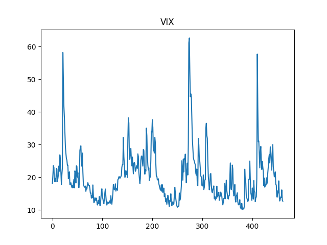
The main data series in this article is Chicago Board of Options Exchange (CBOE) Volatiltiy Index (VIX). This is taken from the Federal Reserve Economic Data (FRED) web site. The main series designed for Standard & Poor 500 started in January 1990. This series is code-named VIXCLS on the FRED web site. Another series starts from January 1986, but was discontinued in November 2021. It is based on a related index, Standard & Poor 100. This series is code named VXOCLS on the FRED web site. For each time series, we consider its monthly average values. When they overlap, these two indices are highly correlated. We unite them in one time series: Jan 1986 – Feb 1990 for VXOCLS and Mar 1990 - Jan 2024 for VIXCLS. This is called . We plot this data 1986–2024 for months in Figure 1 (A).
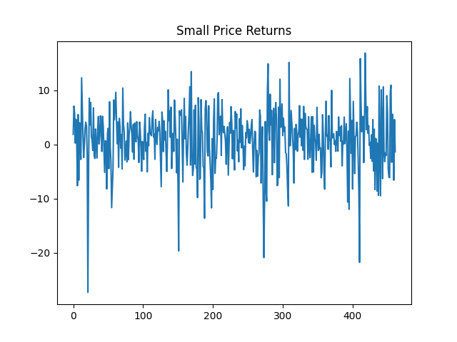
Next, we have data on monthly stock index returns. A capitalization of a stock is its market size (price of one stock times the number of outstanding stocks). We take two portfolios of stocks: Top 30% and Mid 40% (ranked by capitalization). Each portfolio is capitalization-weighted: Each stock in this portfolio is included in proportion to its size. We note that the returns of the Top 30% portfolio closely correspond to that S&P 500 or Russell 1000 (large US stocks), and Mid 40% to Russell 2000 (small US stocks). This is why we call Top 30% Large Stocks and Mid 40% Small Stocks. The data is in percentages. As for the VIX, the data is Jan 1986 – Jun 2024, total months. We consider two versions of returns: price returns, which include only price movements, and total returns, which include dividends. Of course, total returns are always greater than or equal to price returns. Small price returns are on Figure 1 (B).
2.2. Description of statistical functions
Below we analyze whether can reasonably be described as independent identically distributed (IID) Gaussian random variables, or Gaussian white noise. We test separately whether these are: (a) Gaussian; (b) IID. To this end, we compute the following statistical functions of returns . See the background on normality and IID testing in any standard time series textbook, for example [9]: [9, Section 1.4] for testing ACF, and [9, Section 1.5] for normality testing.
| Index Returns | ||||
|---|---|---|---|---|
| Small Total | -0.72/-0.02 | 2.52/-0.40 | 0.0121/0.0096 | 0.0629/0.0038 |
| Large Total | -0.67/-0.11 | 1.73/-0.33 | 0.0072/0.0127 | 0.104/0.0167 |
| Small Price | -0.72/-0.02 | 2.54/-0.4 | 0.0121/0.0101 | 0.0668/0.0043 |
| Large Price | -0.67/-0.11 | 1.75/-0.33 | 0.0072/0.0129 | 0.1145/0.015 |
For (a), we compute skewness and kurtosis . Their well-known definitions are below.
| (4) |
is the empirical th order centered moment, and and are the empirical mean and standard deviation. For i.i.d. , these approximate true skewness and kurtosis of :
| (5) |
For a normal distribution , we have: . Thus if empirical skewness and kurtosis are closer to 0 this implies returns are closer to Gaussian.
For (b), we compute the (empirical) autocorrelation function (ACF) (for ). This is the empirical correlation between and . If are IID, then for every , the theoretical ACF is (for any ). And the empirical ACF is close to this theoretical value, which is . To create a summary statistic, we then compute the -norm (sum of squares) for this ACF. Incidentally, this is the Box-Pierce statistic, see [9, Section 1.4.1] or any other time series textbook.
Furthermore, we do the same for absolute values of returns: . The new ACF is denoted by , and we compute the -norm for this new ACF:
2.3. Results of statistical analysis
In Table 1, we have the results for original (non-normalized) returns and for normalized returns (after dividing by VIX). We see that the skewness and kurtosis for normalized retruns are much closer to zero. In the ACF for original values, there is not much improvement when switching from to . But there is a lot of improvement, judging by the ACF for absolute values. The -norm for these values become much closer to zero.
| Returns | Small Total | Large Total | Small Price | Large Price |
| Mean | 0.075 | 0.072 | 0.069 | 0.062 |
| Stdev | 0.25 | 0.203 | 0.249 | 0.202 |
| Correl | -54% | -53% | -54% | -53% |
| Returns | Small Total | Large Total | Small Price | Large Price |
|---|---|---|---|---|
| Coefficient | 3.6655 | 3.3981 | 3.5628 | 3.2224 |
| Coefficient | -0.1304 | -0.1191 | -0.1316 | -0.1195 |
| Stdev of | 0.2421 | 0.1945 | 0.2416 | 0.1941 |
| Correlation with | -44% | -42% | -44% | -42% |
| Skewness for | 0.022 | 0.024 | 0.026 | 0.026 |
| Kurtosis for | -0.392 | -0.275 | -0.391 | -0.27 |
| 0.009 | 0.0177 | 0.0092 | 0.0177 | |
| 0.0174 | 0.0134 | 0.0177 | 0.0149 |
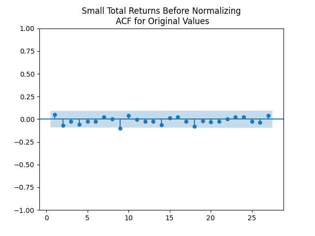
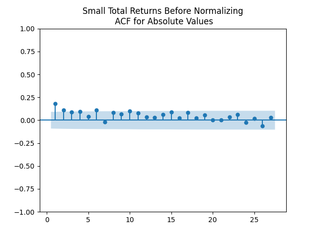
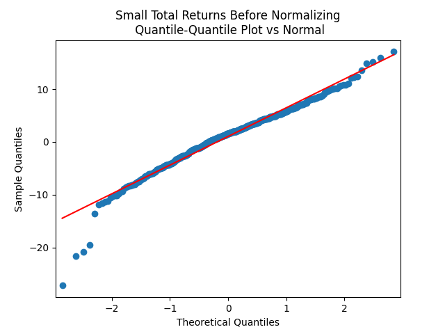
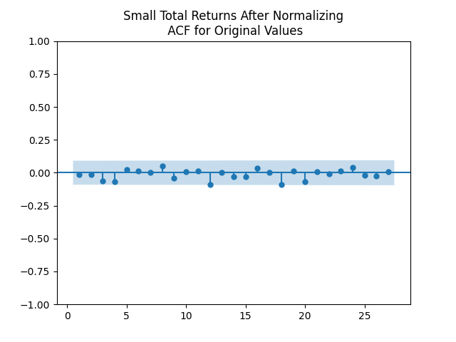
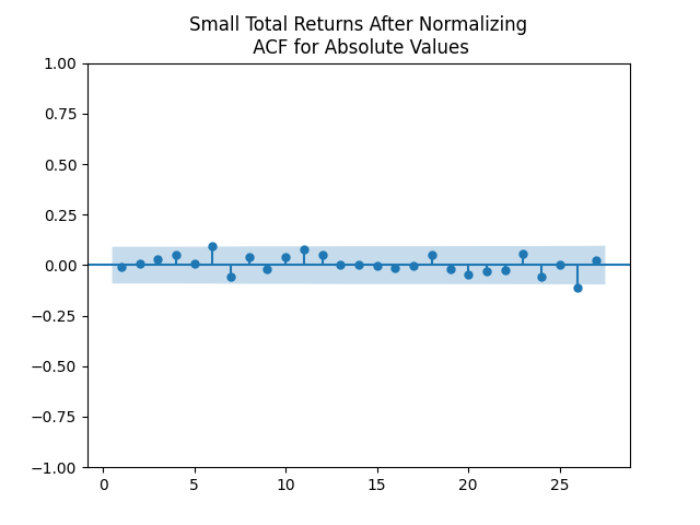
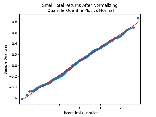
This is supported by the graphs of empirical ACF for returns before and after normalizing, as well as by the quantile-quantile plots vs the normal distribution. In Figure 2, we see ACF for several ; ACF for several ; and the quantile-quantile plot vs the normal distribution, for the original Small Total Returns . Figure 2 contains the same for the normalized version: . Plots for Small Price Returns, Large Total Returns, and Large Price Returns look similarly. One sees that the ACF plots for in Figure 2 (A) and for in Figure 2 (D) look both close to zero, but there is a noticeable difference in the ACF plots for in Figure 2 (B) and for in Figure 2 (E). The former has some values away from zero, but the latter looks closer to zero. Also, the quantile-quantile plots in Figure 2 (C) and (F) show that normalized returns are closer to the normal than non-normalized ones. To the authors, it is a positive surprise that the volatility created from S&P 500 (Large Price Returns) works well also for Small Stocks (Price or Total Returns), and Large Total Returns.
We also refer the reader to a more extensive study [7] of autocorrelation for S&P 500 price returns. They show that raising absolute returns to a power produces more autocorrelation. However, their research is for daily, not monthly returns.
2.4. Complete regression
A more general version of the model (1) for has an intercept:
| (6) |
We can rewrite (6) as follows:
| (7) |
Then we fit this regression for each of the four stock return series: Small Total, Small Price, Large Total, Large Price. The summary is in Table 3. Next, for residuals , their skewness and kurtosis are as small or smaller than the second ones in Table 1. This implies are as well or even better modeled by the normal distribution than normalized returns. The coefficients and are significantly different from zero, with Student -test -values less than . The model (6) will be our main model in the rest of the article.
3. Time Series Analysis of Monthly Average VIX
3.1. The simplest Heston model
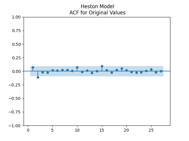
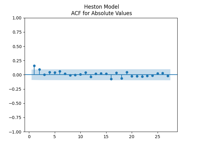
As discussed in the Introduction, the simplest model for VIX is Heston model (2). Fitting this for monthly Jan 1986 – Jun 2024 data gives us , . However, there is a problem. Figure 3 (A, B) has plots of the autocorrelation function (ACF) for innovations and for . These show that are not quite white noise. In particular, ACF with lags 1 and 2 for are outside of the shaded region, corresponding to white noise hypothesis. Thus we switch to find another model.
3.2. Autoregression of order 1 in log scale
As discussed in the Introduction, the VIX is always positive and mean-reverting. Thus it makes sense to use autoregression of order 1 on log scale, as in (3). Rewrite this as
| (8) |
Fitting this for monthly Jan 1986 – Jun 2024 data gives us , (therefore ). The correlation between and is , therefore . The -value for Student -test with zero correlation as null hypothesis is . Note that zero correlation in (8) corresponds to , so becomes a random walk. The Augmented Dickey-Fuller unit root test applied to with 15 lags gives us . Thus we reject the unit root null hypothesis. In sum, the evidence is strongly in favor of mean-reversion in .
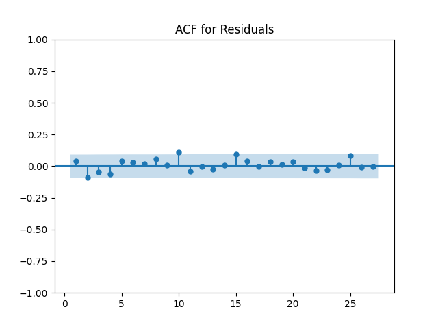
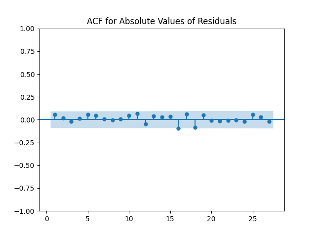
Figure 3 (C, D) has plots of the autocorrelation function (ACF) for innovations and for . These show clearly that can be reasonably modeled as independent identically distributed mean zero random variables. As discussed earlier with regard to stock market returns, we need an additional ACF plot for and are not satisfied with only the ACF plot for . Indeed, it is possible for time series to have zero linear autocorrelation but depend upon the past in a nonlinear way. Stochastic Volatility models described in the Introduction are a perfect example of that, if is independent of the innovations in .
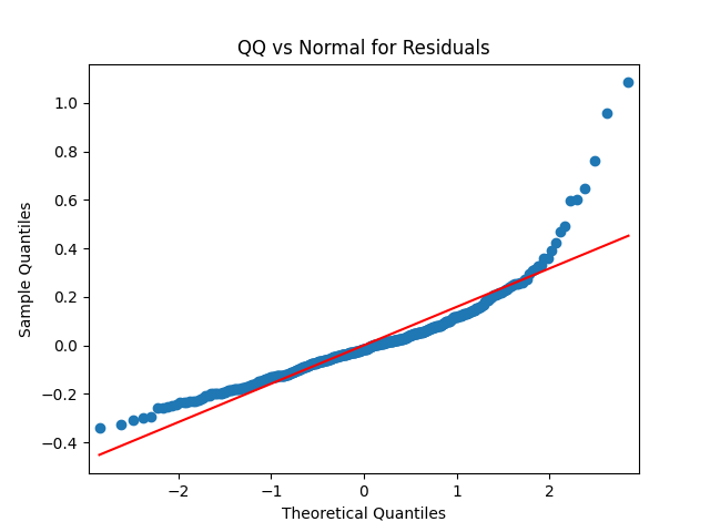
However, the distribution of the innovations is not Gaussian, but has heavier tails. Figure 4 (A) clearly shows this using the quantile-qauntile plot vs the normal distribution. Computed using (4), the skewness of is 2, and the excess kurtosis is 9. Of course, we reject the null normality hypothesis based on Shapiro-Wilk and Jarque-Bera tests.
3.3. Variance-gamma distribution of regression residuals
Instead, we fit variance-gamma distribution using Python package dlaptevVarGamma from GitHub. We use the parametrization from [18], since that Python package uses it as well.
Definition 1.
The variance-gamma (VG), or generalized asymmetric Laplace (GAL), distribution is defined as the distribution of a random variable
| (9) |
where and is independent of and has a gamma distribution with density
Here, has shape parameter , and is rescaled so that . The moment generating function of this distribution is given by
| (10) |
and is well-defined if . More properties on this distribution, along with different parametrizations, are available in [10]. A multivariate version is discussed in [16]. The package dlaptevVarGamma provides the maximum likelihood estimation of parameters, with initial step by method of moments done in [18]. For the residuals from (3), the parameter estimation gives us
| (11) |
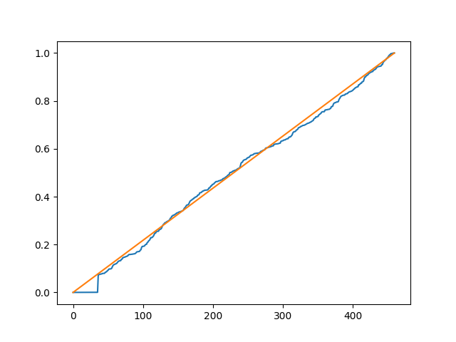
Thus the MGF from (10) is well-defined for . The QQ plot of the residuals vs simulated variance-gamma random variable (9) with parameters (11), and the PP plot of vs this variance-gamma distribution, are given in Figure 4 (B) and (C). They show somewhat good but nor perfect fit though.
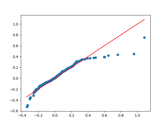
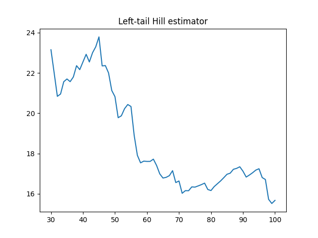
However, we see that the VG model does not fit perfectly. There are problems in the right tail. At least we can estimate left and right tails using Hill estimator from [15] for . We sort these: , and choose the cutoff , and compute the left and right tail estimates and , respectively.
| (12) | ||||
An interesting question is how to choose the cutoff . We plot vs and vs , see Figure 5. We choose and get and . Therefore,
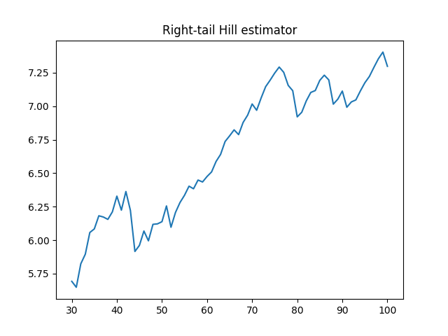
To conclude: Statistical analysis shows that is well-modeled by mean-reverting autoregression of order . The residuals of this autoregression are independent identically distributed but not Gaussian. However, they have exponential-like tails, with for for some .
4. Combined Model of Volatility and Stock Returns
As discussed in Section 2, can be modeled as IID normal random variables: . As discussed in Section 3, however, are IID mean-zero but not normal.
4.1. Finite moments for volatility
First, let us deal just with the volatility modeled by the log Heston model (3).
Assumption 1.
In (3), , and are independent identically distributed with and for a certain ; the initial condition is independent of all , with .
Lemma 1.
Under Assumption 1, we have: . Moreover, there exists a unique stationary distribution , and the variable satisfies .
Proof.
Without loss of generality, assume . We rewrite (3) as
Write this in exponential form:
Apply the expectation, and use independence of :
| (14) |
By Assumption 1, is well-defined for , in particular for since . Also, , , . By Taylor’s formula, we get: As ,
| (15) |
Next, we take logarithms in (14):
| (16) |
As , we have: , and . Moreover, for . Applying (15), we get: as . Therefore, both series below converge:
Thus, the sequence (16) converges as . Every converging sequence is bounded. This proves the first claim of Lemma 1. Let us show the second claim. This stationary distribution is, in fact, the weak limit: . By the Skorohod representation theorem, we can switch to almost sure convergence on a new probability space. But . By Fatou’s lemma, we get: . This proves the second claim of Lemma 1. ∎
4.2. Finite moments for stock returns
Now, we turn back to stock index returns . Under Assumption 1, we prove they have finite moments up to a certain order. This captures a well-known property of stock market returns: Pareto-like tails, first noted by Fama in [8]. However, the second moment of real-world stock returns is finite. This follows from Theorem 1 for and the empirical analysis in the previous section.
Assumption 2.
are IID random vectors with mean , while the marginal distribution of is Gaussian.
We do not require and to be independent or even uncorrelated, though this would simplify computations; see later.
Theorem 1.
Proof.
That the system has a stationary solution is clear. Now, by Minkowski’s inequality,
| (17) |
We already have . It suffices to prove . Pick and let be such that . Then by H’́older’s inequality,
| (18) |
where is the th absolute moment of the random variable : . Therefore, this th moment of is finite. We can take in (17) and (18), and repeat the proof. The same proof works for instead of . ∎
4.3. Limit theorems
Below, under additional assumptions, we state and prove the Law of Large Numbers and the Central Limit Theorem for monthly stock index returns. Since these assumptions are borne out by real-world data, we see that the real-world property is reproduced: Over longer time periods, returns are closer to normal. See discussion of this in [2] and references therein.
Assumption 3.
The distribution of has strictly positive density on the entire real line. Moreover, .
Theorem 2.
Proof.
Under Assumptions 1, 2, 3, the process is Markov on the state space with -step transition function . The Markovian property follows from the fact that is a one-to-one function of . Indeed, is a Markov process on . This is because is an autoregression of order , and are IID. Thus it is a linear model. What is more, this process has a unique stationary distribution, and is -uniformly ergodic, with . See the definitions and results in [17, Chapter 16]. The Law of Large Numbers and the Central Limit Theorem follow from [17, Chapter 17]. ∎
5. Conclusion
We propose and fit a log-Heston model for monthly average volatility and stock idnex returns. It fits actual financial data well. This model exhibits good long-term properties: stationarity and mean-reversion. It captures a well-known property of real-world stock idnex returns: Pareto-like tails. For this, we need innovations in this log-Heston model which have tails heavier than Gaussian. Future research might include finding bivariate distributions which are a good fit for innovations . Also, it is important to analyze other stock indices, such as Value, Growth, or international.
References
- [1] Torben G. Andersen, Tim Bollerslev (1998). Answering the Skeptics: Yes, Standard Volatility Models do Provide Accurate Forecasts. International Economic Review 39 (4), 885–905.
- [2] Antonios Antypas, Phoebe Koundouri, Nikolaos Kourogenis (2013). Aggregational Gaussianity and Barely Infinite Variance in Financial Returns. Journal of Empirical Finance 20, 102–108.
- [3] Geert Bekaert, Marie Hoerova (2014). The VIX, the Variance Premium and Stock Market Volatility. Journal of Econometrics 183, 181–192.
- [4] Lorenzo Bergomi. Stochastic Volatility Modeling. Chapman & Hall/CRC.
- [5] Tim Bollerslev (1986). Generalized Autoregressive Conditional Heteroskedasticity. Journal of Econometrics 31 (3), 307–327.
- [6] M. Angeles Carnero, Daniel Pena, Esther Ruiz (2004). Persistence and Kurtosis in GARCH and Stochastic Volatility Models. Journal of Financial Econometrics 2 (2), 319–342.
- [7] Zhuanxin Ding, Clive W. J. Granger, Robert F. Engle (1993). A Long Memory Property of Stock Market Returns and a New Model. Journal of Empirical Finance 1, 83–106.
- [8] Eugene F. Fama (1963). Mandelbrot and the Stable Paretian Hypothesis. The Journal of Business 36 (4), 420–429.
- [9] Jianqing Fan, Qiwei Yao (2017). The Elements of Financial Econometrics. Cambridge University Press.
- [10] Adrian Fischer, Robert E. Gaunt, Andrey Sarantsev (2023). The Variance-Gamma Distribution: A Review. arXiv:2303.05615.
- [11] Christian Francq, Jean-Michel Zakoian (2019). GARCH Models: Structure, Statistical Inference and Financial Applications. 2nd Edition, Wiley.
- [12] Christian Francq, Olivier Wintenberger, Jean-Michel Zakoian (2013). GARCH Models Without Positivity Constraints: Exponential or Log GARCH? Journal of Econometrics 177 (1), 34–46.
- [13] Hafida Guerbyenne, Faycal Hamdi, Malika Hamrat (2024). The log-GARCH Stochastic Volatility Model. Statistics & Probability Letters 214, 110185.
- [14] Steven L. Heston (1993). A Closed-Form Solution for Options with Stochastic Volatility with Applications to Bond and Currency Options. The Review of Financial Studies 6, 327–343.
- [15] Bruce M. Hill (1975). A Simple General Approach to Inference About the Tail of a Distribution. Annals of Statistics 3 (5), 1163–1174.
- [16] Tomasz J. Kozubowski, Krzysztof Podgórski, Igor Rychlik (2013). Multivariate Generalized Laplace Distribution and Related Random Fields. Journal of Multivariate Analysis 113, 59–72.
- [17] Sean P. Meyn, Richard L. Tweedie (2009). Markov Chains and Stochastic Stability.Second edition, Springer.
- [18] Eugene Seneta (2004). Fitting the Variance-Gamma Model to Financial Data. Journal of Applied Probability 41(A), 177-187.
- [19] Elias M. Stein, Jeremy C. Stein (1991). Stock Price Distributions with Stochastic Volatility: An Analytic Approach. The Review of Financial Studies 4, (4), 727–752.
- [20] R. E. Whaley (2000). The Investor Fear Gauge. Journal of Portfolio Management 12–17.