First results from the JWST Early Release Science Program Q3D: AGN photoionization and shock ionization in a red quasar at z = 0.4

Abstract

Red quasars, often associated with potent [O III] outflows on both galactic and circumgalactic scales, may play a pivotal role in galactic evolution and black hole feedback. In this work, we explore the [Fe II] emission in one such quasar at $z=0.4352$—F2M J110648.32+480712.3—using the integral field unit (IFU) mode of the Near Infrared Spectrograph (NIRSpec) aboard the James Webb Space Telescope (JWST). Our observations reveal clumpy [Fe II] gas located to the south of the quasar. By comparing the kinematics of [Fe II] and [O III], we find that the clumpy [Fe II] gas in the southeast and southwest aligns with the outflow, exhibiting similar median velocities up to v₅₀ $=$ 1200 km s^-1 and high velocity widths W₈₀ $>$ 1000 km s^-1. In contrast, the [Fe II] gas to the south shows kinematics inconsistent with the outflow, with W₈₀$\sim$ 500 km s^-1, significantly smaller than the [O III] at the same location, suggesting that the [Fe II] may be confined within the host galaxy. Utilizing standard emission-line diagnostic ratios, we map the ionization sources of the gas. According to the MAPPINGS III shock models for [Fe II]/Pa$\beta$, the regions to the southwest and southeast of the quasar are primarily photoionized. Conversely, the [Fe II] emission to the south is likely excited by shocks generated by the back-pressure of the outflow on the galaxy disk, a direct signature of the impact of the quasar on its host.

1 Introduction

One crucial aspect of quasar feedback is the interplay between quasar-driven winds/outflows and the interstellar medium (ISM) within the host galaxy (Fabian, 2012). These powerful winds impart a substantial amount of energy onto the surrounding ISM, leading to the formation of shock waves that can have profound consequences for the galaxy’s star formation capacity, either by dispersing or reheating its cold gas reservoir (Silk & Rees, 1998; King, 2003; Kormendy & Ho, 2013; King & Pounds, 2015; Veilleux et al., 2020). Consequently, the identification and characterization of shock signatures have long been sought after as a diagnostic tool for understanding the interaction between quasar winds and the ISM.

Historically, evidence for this feedback between quasar driven winds/outflows and shock-heated regions has been primarily indirect and observed in lower luminosity active galactic nuclei (AGN) residing in nearby galaxies, as illustrated in Allen et al. (1999). For example, Zakamska & Greene (2014) use weaker optical lines as indirect shock signatures in a set of obscured luminous quasars, interpreting the similar velocities between these emissions and the outflows as evidence of quasar-driven winds propagating into the ISM of the host galaxy. The advent of integral field spectroscopy has ushered in an era marked by the accumulation of direct, spatially resolved evidence for shock signatures beyond the quasar’s illumination cone. This is seen in Riffel et al. (2021b), who provide direct evidence of outflow driven shock ionization in regions orthogonal to the ionization axis in Mrk79 and Mrk348. Similarly, Leung et al. (2021) discovered a region of low-ionization, high dispersion gas in Mrk273, displaying an orthogonal orientation to the photoionization cone. These findings have also been extended beyond the local universe more recently, as Vayner et al. (2023) find evidence for shock ionization induced by a quasar-driven outflow in a z = 3 redshift source, J1652, through JWST NIRSpec data.

The low-ionization, near-infrared emission lines of [Fe II] are strong in regions of fast shocks, effectively tracing warm and cold interstellar medium phases (Oliva et al., 1989). These lines frequently serve as tracers to identify shocked regions. However, unraveling the origin of [Fe II] is complicated. While prior studies suggest quasar photoionization either directly or through quasar-driven outflows to dominate ionization due to high temperatures of the ionized regions (Mouri et al., 2000), other mechanisms could potentially affect the interpretation of [Fe II] in these regions. For instance, several studies find [Fe II] emission to arise from star formation processes, where supernovae release vast amounts of energy, launching powerful shockwaves throughout the ISM (Reach et al., 2002, 2005; Koo et al., 2007; Lee et al., 2009). The increased gas phase abundance of iron from dust grain destruction combined with other ionizing effects is responsible for large [Fe II] enhancements as observed in several supernovae. Additionally, hydrodynamical simulations (Mukherjee et al., 2016; Wagner et al., 2016) and observational studies (Lacy et al., 2017; Zovaro et al., 2019) cite radio jets as potential [Fe II] production mechanisms. These jets propagate into inhomogeneous ISM to form energy-driven bubbles that ionize the surrounding medium and create bow shocks.

The emission of [Fe II] exhibits a correlation with the star formation rate, enabling differentiation between contributions from quasar photoionization and those originating from star formation processes (Graham et al., 1987; Koo & Lee, 2015). If the detected [Fe II] emission is in excess of what is expected based on star formation alone, it can be attributed to the influence of the quasar.

We obtained integral field spectroscopy data of [Fe II] with the James Webb NIRSpec instrument as part of the Q3D Early Release Science program. The Q3D program is dedicated to the exploration of quasar feedback processes in host galaxies and development of a scientific tool, q3dfit (Rupke et al., 2023a). This software provides the scientific community with more convenient spectral mapping and point spread function (PSF) decomposition of the JWST IFU data to obtain science-ready products that can be used for the analysis of quasars and their galaxy hosts on different redshifts. F2M J110648.32+480712.3, hereafter F2M1106, is one of three quasars we use to train and test the q3dfit package.

In this paper, we begin by summarizing all known properties of F2M1106 in Section 2. Section 3 details the observational setup, data reduction, and analysis of the [Fe II] emission in the JWST NIRSpec dataset. In Section 4, we discuss the origin of [Fe II] ionization. We summarize in Section 5. Throughout this paper we adopt the cosmological parameters H₀ = 69.6 km s^-1 Mpc^-1, $\Omega_{M}$ = 0.286, and $\Omega_{\Lambda}$ = 0.714 of the flat $\Lambda$CDM model (Bennett et al., 2014).

2 F2M1106

2.1 Previous Studies

F2M1106 is a red quasar originally identified by Glikman et al. (2012) and confirmed by them using optical spectroscopy. It has a redshift of $z=0.4352$ as determined by Keck KCWI based on stellar kinematics (Rupke et al., in prep). The initial identification of the object was based on its detection as a luminous radio source in the Faint Images of the Radio Sky at Twenty-Centimeters survey (FIRST; White et al. 1997) indicating the presence of an active nucleus and red colors in the Two Micron All Sky Survey (2MASS E(B-V) = 0.44; Skrutskie et al. 2006) suggesting high levels of reddening. A broader coverage optical spectrum of the source was further obtained by the Baryon Oscillation Spectroscopic Survey (BOSS) of the Sloan Digital Sky Survey (SDSS; Eisenstein et al. 2011). It shows broad emission lines of H$\alpha$, H$\beta$ and H$\gamma$, a strong contribution from FeII (Boroson & Green, 1992) which was analyzed by Hu et al. (2008) as part of a larger sample and flat continuum ($F_{\lambda}\propto\lambda^{0}$, unlike the optical continuum of unobscured quasars with $F_{\lambda}\propto\lambda^{-1.56}$, Vanden Berk et al. 2001).

The quasar is not detected in a 6 ksec Chandra exposure (Glikman et al., 2024), which is not unusual for red and obscured quasars, even intrinsically luminous, due to the high levels of X-ray absorption (LaMassa et al., 2016; Glikman et al., 2017). The radio source, with flux $F_{\nu}=10.6\pm 0.14$ mJy at 1.4 GHz (White et al., 1997), is consistent with being point-like at the 5″ spatial resolution of FIRST. The flux at 150 MHz obtained in LOFAR Two-metre Sky Survey (Shimwell et al., 2017) is $F_{\nu}=75\pm 15$ mJy, suggesting an overall spectral index of $\alpha=-0.88$, standard for optically thin synchrotron radiation. There is no evidence for a strong radio core emission which would be indicative of a compact jet.

Shen et al. (2023) obtained optical integral field spectroscopy of the object with the Gemini Multi-Object Spectrograph and used spatially resolved kinematic mapping of [O III]$\lambda$5007 Å to discover a large ($\sim 40$ kpc from end to end) ionized nebula around the target. The gas shows an organized motion with a velocity difference between the redshifted and the blueshifted sides of over 1000 km s^-1. Shen et al. (2023) interpret these data as a powerful quasar-driven galactic outflow, possibly in the form of ‘super-bubbles’ (Greene et al., 2012) which are expected to occur when a wind breaks out of a dense environment of the host galaxy and into the lower density circumgalactic halo, with the galaxy’s morphology influencing how the superbubbles evolve. Observations with HST reveal that low-redshift red quasars as a population are typically found in major mergers (Urrutia et al., 2008); however, no HST data are available for our target. While the host galaxy was not detected either in the integrated optical spectrum or in the Gemini spatially resolved spectroscopy, it is detected in the blue part of the optical range using deep Keck Cosmic Web Imager integral field spectroscopy and spectral PSF subtraction (Rupke et al., in prep).

Integral field spectroscopy of F2M1106 using the Mid-InfraRed Instrument (MIRI) on JWST detected the [O III]$\lambda$5007 Å outflow in the light of [S IV] 10.51 $\mu$m (Rupke et al., 2023b). This transition traces similar physical conditions to [O III]$\lambda$5007 Å, but at much longer wavelengths. The comparison reveals differential dust reddening in the approaching and receding sides of the outflow, suggesting that the latter is obscured by the host galaxy at $A_{V}\leq 2.0$ mag, discussed further in Section 3.4.

2.2 Spectral Energy Distribution

Figure 1: Top: Dust opacity curves (Weingartner & Draine, 2001), each with a different Milky Way dust extinction coefficient. Bottom: Our spectral energy distribution (SED) models for F2M1106 multiwavelength photometry (error bars are present but small). The intrinsic AGN continuum experiences considerable reddening with observed UV/ optical excess in the SDSS u band and GALEX NUV. We utilize a model consisting of a blue quasar (Polletta et al., 2007) (in blue), a dusty torus (not pictured; Weingartner & Draine (2001)), and with contributions from the host galaxy (purple) and quasar scattered light (dashed blue). Three fits of this model are depicted (in various shades of red), each corresponding to the three distinct dust models illustrated in the upper plot. We find the scattered light component to comprise roughly 6$\%$ of the intrinsic UV emission.

We model the spectral energy distribution (SED) spanning from the optical to far-infrared wavelengths. The SED incorporates photometric data obtained from various surveys and instruments, including the Galaxy Evolution Explorer (GALEX) near-ultraviolet (NUV) band (Martin et al., 2005), SDSS ugriz bands in the optical, 2MASS J-, H-, K-bands, and Wide-field Infrared Survey Explorer (WISE) W1–W4 channels (Wright et al., 2010). Additionally, we obtain 3$\sigma$ upper limits in the far-infrared from Stratospheric Observatory for Infrared Astronomy (SOFIA) observations using the HAWC+ C (62 µm rest-frame) and D (107 µm rest-frame) bands (Harper et al., 2018), which are observed for 67 min and 77 min respectively.

Red quasars, typically exhibiting high luminosities (i.e $\nu$L_5µm = 10^45.5 erg s^-1) and reddening ($A_{V}\sim 1-20$ mag; Glikman et al. 2007; Urrutia et al. 2012; Ishikawa et al. 2021; Glikman et al. 2022), outshine their host galaxies in the rest-frame optical. Their SEDs are often well characterized by reddening an unobscured quasar template spectrum using a ‘screen of cold dust’ approximation with a standard dust extinction curve. We find similarly high WISE luminosities for our object and initially consider a model with a blue quasar (Polletta et al., 2007) subject to varying levels of dust absorption (Weingartner & Draine, 2001). However, the fitting proves inadequate in explaining the observed blue excess, particularly prominent in the SDSS u and GALEX NUV bands. In the rest-frame UV, the quasar light is heavily extinguished and the host galaxy, particularly the young stars within it, may contribute to the overall flux density (Jahnke et al., 2004). Additionally, the UV-emitting component could arise from a fraction of quasar light scattering off of the ISM on scales larger than the obscuring material (Zakamska et al., 2005, 2006).

From Keck KCWI observations, we know the host galaxy flux to be in the range 16-33$\%$ of the total quasar light over the rest frame range 2400–3900 Å (Rupke et al. in prep.). We scale the template of an active star forming galaxy (Polletta et al., 2007) assuming the host contributes 25$\%$ of the total quasar light in this range (the average) and compute a star formation rate upper limit for the host of $\sim$132 M_⊙ yr^-1 using the 8–1000 µm infrared luminosity (Bell, 2003). Because there is a wide range of infrared-to-UV flux ratios amongst star-forming galaxy templates and because we do not have good far-infrared / submm coverage of the SED, this is only an estimate.

The remaining UV contribution is accounted for by a blue quasar component scattered into our line of sight with efficiency f_scat$=$6$\%$, which is consistent with previous studies who generally quote efficiencies of a few per cent. For example, Young et al. (2009) find a scattering efficiency of 6.25$\%$ for NGC 1068 while Greene et al. (2014) find an efficiency of 3$\%$ for radio quiet quasar SDSS J135646.10+102609.0. Obied et al. (2016) analyze Hubble Space Telescope observations of 20 luminous obscured quasars between 0.24 $<$ z $<$ 0.65 and find a median scattering efficiency of 2.3$\%$.

The resulting model, which includes a blue quasar, cold screen of dust, a star forming galaxy, and a quasar scattered component, is illustrated in Figure 1. Our analysis yields a moderate continuum extinction magnitude, A_V,SED $=$ 3.2 $\pm$ 0.8 mag. Estimating the bolometric luminosity using the wavelength-dependent bolometric correction for Type 1 quasars (MacArthur et al., 2004; Richards et al., 2006), we derive a value of L_bol $=$ 10^46.5±0.1 ergs s^-1. We choose not to perform a more sophisticated multi-parametric SED fit because the poor coverage of the SED in the far-infrared precludes an independent measurement of the SFR, because the scattered light contribution and the UV-bright star formation are degenerate (Greene et al., 2024), and because in red quasars specifically the standard packages tend to result in an overly massive fit to the host galaxy as they do not reproduce well the near-infrared portion of the quasar emission.

2.3 Optical Integrated Spectrum Analysis

We employ the PyQSOFit code (v2.0) developed by Guo et al. (2018) to fit the optical nuclear spectrum obtained from SDSS. The fitting procedure is conducted in the rest frame using a $\chi^{2}$-based methodology. Following the modeling of the continuum through a third order polynomial function and the subsequent subtraction of the continuum emission and an optical FeII template included in the package, we proceed to model the emission lines, including H$\alpha$ and H$\beta$, utilizing a combination of narrow and broad Gaussian components. Within the H$\alpha$+[N II]+[S II] complex, all forbidden lines and the narrow component of H$\alpha$ have the same velocity centroids and widths. Broad components like H$\alpha$ and H$\beta$ vary independently. For accurate flux scaling, fixed flux ratios are enforced where appropriate, such as between [O III]$\lambda$4959 Å and [O III]$\lambda$5007 Å. The results are shown in Figure 2, with the uncertainties determined through a Monte Carlo procedure.

[O III] emission is characterized by unusually high velocity width, as appropriate for a quasar with an extremely high-velocity circumgalactic outflow (Shen et al., 2023). But we find that H$\alpha$ and H$\beta$ are significantly broader than any forbidden lines in the spectrum and we classify F2M1106 as a Type 1 AGN. We find the [O III] doublet to be blended together with H$\beta$ and explore the possibility of these lines sharing similar kinematic structures, potentially indicating emission from the same physical region. However, we observe distinct kinematic signatures; the [O III] doublet exhibits a double-peaked, redshifted and blueshifted structure, contrasting with H$\beta$, which predominantly displays an unshifted broad component alongside a weaker and narrower blueshifted component. F2M1106 also has strong FeII emission (Hu et al., 2008), indicating that it may be a high-Eddington source (Boroson & Green, 1992).

2.4 Nuclear Extinction and Black Hole Mass Estimation

We determine the extinction in the nuclear region in this object using the Balmer emission line ratio (using the broad H$\alpha$ and H$\beta$ components derived from fitting), which is shaped by the equilibrium between photoionization and recombination. Case B recombination in hydrogen sets a lower theoretical bound on H$\alpha$/H$\beta$ at 2.98 in dust-free gas at T_e $=$ 10⁴ K (Dopita et al., 2003). In unobscured Type 1 quasars, this ratio peaks at 3.3 (Kim et al., 2006), and an elevated ratio beyond this suggests dust extinction. We estimate A_V using the relation given in Riffel et al. (2021a) to be 2.4 $\pm$ 0.3 mag, which is consistent with the extinction derived from the SED-fitting technique and with observations in other red quasars (Banerji et al., 2015; Fawcett et al., 2023).

We assume that the gas within the broad-line region surrounding the black hole is virialized (Peterson et al., 2004) to estimate the black hole mass. The velocity of the gas is deduced from the width of the broad H$\alpha$ emission line, which is less affected than other tracers such as H$\beta$ by dust extinction, while the associated rest-frame line luminosity L₅₁₀₀, which we correct for the extinction, serves as a proxy for the size of the broad-line region. Using the virial scaling relation from Shen & Liu (2012), we derive a black hole mass of M_BH = 10^9.5±0.2 M_⊙. The uncertainty is based solely on measurement errors from the MCMC-produced H$\alpha$ broad line FWHM, and does not account for potential systematic uncertainties. The black hole mass estimate could vary by an order of magnitude depending on the calibration methods employed for the emission lines (Bertemes et al., 2024). We find this result to be similar to the black hole masses quoted for this object in Hu et al. (2008) and Rupke et. al. in prep, who determine the mass to be $\sim$10^9.1 M_⊙ using H$\beta$ and MgII respectively. The resulting Eddington luminosity is L_Edd $=$ 10^47.5±0.8 erg s^-1 and the Eddington ratio, using the bolometric luminosity calculated in Section (2.2), is log $\lambda_{Edd}$ $=$ –1.0$\pm$ 0.3.

Figure 2: PyQSOFit fits to optical Sloan Digital Sky Survey spectra of F2M1106. The upper panel shows the fits to the entire spectrum. The continuum is shown in orange, the optical FeII contribution is in aqua. In the bottom panels: (left) the H$\beta$, [O III] $\lambda$4959, and [O III] $\lambda$5007 emission features. The [O III] lines require two Gaussian components during fitting while H$\beta$ favors an unshifted broad component and a blueshifted broad component. (right) H$\alpha$ fit with two components. Other lines fit here are [N II] $\lambda$6549, [N II] $\lambda$6585, [S II] $\lambda$6718, and [S II] $\lambda$6732.

3 Analysis of JWST Data

3.1 Observational Design and Data Reduction

James Webb Space Telescope NIRSpec integral field spectroscopy (Jakobsen et al., 2022) observations were acquired on November 13, 2022 using both the G395H grating/ 290LP filter and the G235H grating/ 170LP filter. We employed a nine-point dither pattern during observation to improve the spatial sampling of the PSF. An additional exposure at the first dither position with the micro-shutter assembly (MSA) closed was taken to constrain any light contamination from bright objects in the instrument’s field of view and remove it in the case of failed open shutters. Per detector, the effective exposure time per integration for the source was 233.422 s, with a total on-source exposure time of 2100.798 s.

We reduced the data using Space Telescope’s JWST pipeline version 1.14.0 in conjunction with the jwst_1223.pmap version of the calibration reference files. In the initial stage, which encompasses standard infrared detector processing of the uncalibrated files, the pipeline subtracts the dark current, flags the data quality, and conducts an initial iteration of cosmic ray removal. Prior to advancing to the subsequent stage, we apply a band correction to mitigate significant instrument-induced variations across detectors and grating/filter combinations. The resulting rate files obtained from this stage were then fed into the second stage of the pipeline.

In the second stage, the pipeline assigns each frame a world coordinate system, followed by background subtraction, flat-fielding, and flux calibration. Additionally, this stage converted the 2D spectra into a 3D data cube through the execution of the “cube build” routine. We also identified and accounted for imprints generated by the open NIRSpec micro-shutters, as well as flagged and excluded any defective pixels. Finally, we execute the last stage of the pipeline to combine the exposures obtained from different dither positions utilizing the 3D emsm algorithm. We applied a final three sigma clipping method to remove residual cosmic rays, resulting in the production of four data cubes (two per filter associated with the detectors used). Each data cube posseses a pixel scale of 0.1″ and spans specific wavelength ranges: 1.65 µm – 2.40 µm, 2.48 µm – 3.16 µm, 2.67 µm – 4.06 µm, and 4.17 µm – 5.27 µm, respectively.

Parameter	Value
MBH	109.5±0.2 M⊙
Lbol	1046.5±0.1 erg s-1
LEdd	1047.5±0.7 erg s-1
log $\lambda$Edd	–1.0 $\pm$ 0.3
AV,BAL	2.4 $\pm$ 0.3 mag
AV,SED	3.2 $\pm$ 0.8 mag

Table 1: F2M1106 Properties

A significant challenge in studying extended emission in a quasar is the decomposition of the host galaxy from its central quasar. While JWST has high enough spatial resolution to enable studies of quasar hosts at higher redshifts, issues like surface brightness dimming and the quasar’s bright PSF persist. The q3dfit tool (Rupke et al., 2023a), an adapted and extended iteration of IFSFIT (Rupke, 2014; Rupke et al., 2017), presents a promising avenue for effectively modeling and mitigating the influence of the quasar PSF, thereby unveiling the extended emission (Wylezalek et al., 2022; Vayner et al., 2023; Veilleux et al., 2023). While Pa$\beta$, another line of interest, is detected near the nucleus, we do not observe nuclear [Fe II]; therefore, in much of the subsequent [Fe II]-focused analysis, we do not subtract a bright central source. The exception is Section 4.3, where we analyze both [Fe II] and Pa$\beta$ with and without PSF subtraction.

We use q3dfit v1.1.4 for both cases. For the PSF-subtracted case, we identify the brightest spaxel as the central quasar and subtract it from the data prior to fitting each resulting spaxel with a model consisting of a third-order polynomial and emission lines. The non-PSF subtracted case directly fits each spaxel with the same spectral model without any prior subtraction.

3.2 [FeII] $\&$ Pa$\beta$ Morphology and Fitting

Figure 3: (a) JWST NIRSpec [Fe II] 1.6440 µm surface brightness map. The quasar is indicated by a black star, with representative spaxels A, B, and C selected. (b) Extracted spectra from these spaxels are shown in black, with Gaussian fits to the features in red and the individual Gaussian profiles in dotted magenta. The spectra include the [Fe II] 1.2570, [Fe II] 1.2791, [Fe II] 1.6440 µm, and Pa$\beta$ lines. For spaxel C, a second broad Gaussian component is present for the [Fe II] 1.2791 µm and Pa$\beta$ complex, but it has a lower flux amplitude and is cut off from the shown spectrum. (c, d, e) Surface brightness maps of the [Fe II] 1.2570, [Fe II] 1.2791 µm, and total Pa$\beta$ (broad $+$ narrow component) lines, respectively, from left to right. These maps share the same spatial coordinates and color scale as the [Fe II] 1.6440 µm map in (a). Additionally, cyan contours in (b), (c), and (d) represent the [Fe II] 1.6440 µm emitting region for reference.

Figure 3 presents examples of the emission line profiles for the [Fe II] lines at 1.2570, 1.2791, and 1.6440 µm, as well as for Pa$\beta$ (1.2822 µm), taken from individual spaxels A, B, and C, along with their best-fit models in these representative regions. During fitting, we measure velocities relative to the host galaxy redshift, z = 0.4352.

The [Fe II] lines, sharing the same ionization state of iron and similar excitation energies (7.87 eV), should exhibit shared kinematic properties and could be kinematically tied – i.e., fit with the same velocity dispersion and net offset (Zakamska et al., 2016a). In practice, the [Fe II] 1.2570 µm line shows a lower velocity dispersion than [Fe II] 1.6440µm, likely due to a lower signal-to-noise ratio (SNR) at that wavelength across the IFU cube. Specifically, the SNR for spaxels A, B, and C are approximately 5, 3, and 7 for [Fe II] 1.2570 µm, and approximately 11, 9, and 18 for [Fe II] 1.6440 µm. Additionally, [Fe II] 1.2570 µm is not detected to the south of the quasar (around spaxel B), where other [Fe II] lines and Pa$\beta$ are present. Due to the contamination of the [Fe II] 1.2791 µm line in the Pa$\beta$ profile, which is otherwise the brightest in our spectra, we kinematically tie the [Fe II] 1.2791 µm and Pa$\beta$ lines to the [Fe II] 1.6440 µm line during fitting. The [Fe II] 1.2570 µm line, with its lower SNR and differing velocity dispersion, was fit separately. We find a single Gaussian fit to be sufficient for these lines.

Figure 3 presents the surface brightness maps produced by q3dfit for the emission features. From these maps, we observe that there is a clumpy morphology of the [Fe II] 1.6440 µm emission concentrated to the south of the quasar within the NIRSpec field of view. The Pa$\beta$ map, in contrast, shows a continuous distribution, with the central part dominated by the broad nuclear emission and narrower lines in areas where we detect [Fe II]. The [Fe II] 1.2791 µm emission also appears clumpy, concentrated to the southeast and the south of the quasar, although some emission to the southwest may be missed due to its blending with the broad Pa$\beta$ profile. Additionally, the [Fe II] 1.2570 µm emission is observed in clumps to the southwest and southeast of the quasar.

3.3 Comparison with the [O III] Outflow

Figure 4: (row (a), left) v₅₀ map of JWST NIRSpec [Fe II] 1.6440 µm. (row (a), right) v₅₀ map of Gemini GMOS [O III] $\lambda$5007 Å. Row (b) similarly plots for the W₈₀ maps of [Fe II] (left) and [O III] in km s^-1 (right) respectively.

The outflow in F2M1106 was previously detected via [O III]$\lambda$5007 Å by Shen et al. (2023). Here, we compare the properties of [Fe II] 1.6440 µm and [O III] as illustrated in Figure 4 to determine if [Fe II] is associated with the outflow.

Figure 4 reveals that the velocities of the [Fe II] gas consist of two major components. One component is a redshifted nebula in the southeast of the NIRSpec field of view with a median velocity ranging from $\sim$50 km s^-1 to 1100 km s^-1. The other component is a blueshifted nebula towards the southwest with v₅₀ ranging from around $\sim-$1200 km s^-1 to 0 km s^-1. These high velocities exceed the gravitational potential limits, as galaxy rotation velocities typically remain within a few hundred km s^-1 (Reunanen et al., 2002, 2003). This discrepancy between the velocity of ionized gas and the rotational velocity of the host galaxy is further supported by observations of the stellar component of the host galaxy (Rupke et al., in prep), which exhibits a rotational field with inverse velocity gradients (i.e., blueshifted to the east and redshifted to the west).

Additionally, the velocity values (v₅₀) and the orientation of the [Fe II] closely match the [O III] outflow. Therefore, we conclude that a majority of the [Fe II] is part of the outflow and not related to the galaxy’s rotation. Figure 4 also presents a comparison of the [Fe II] and [O III] W₈₀ values, which represent the velocity width encompassing 80$\%$ of the total flux. While this parameter closely resembles the FWHM for a purely Gaussian profile, W₈₀ is more sensitive to the broad bases of non-Gaussian emission line profiles such as wings, making it suitable for analyzing high-velocity motions, including outflows and outflow-impacted emission (Liu et al., 2013; Zakamska & Greene, 2014; Harrison et al., 2014).

Overall, most regions of the nebula show similar W₈₀ values, with both [Fe II] and [O III] exhibiting high W₈₀ velocities $>$ 1000 km s^-1 (seen as a bright yellow “band” in the [O III]). Shen et al. (2023) interpret this “band” as resulting from the overlap of the receding and approaching sides of the outflow, as indicated by the presence of both redshifted and blueshifted components in this region in the v₅₀ map. This is consistent with the findings of Liu et al. (2024), who observe localized regions of high dispersion in Pa$\alpha$—another outflow tracer—at the spatial resolution of the JWST observations. However, some notable differences between [Fe II] and [O III] kinematics emerge. Not all spaxels for [Fe II] exhibit high W₈₀ values within this region. Specifically, towards the south and southeast, the [Fe II] component in a few spaxels appears narrower compared to the [O III] ($\sim$460 km s^-1 for the [Fe II] vs $\sim$1630 km s^-1 for the [O III] in the south and $\sim$590 km s^-1 vs $\sim$1600 km s^-1 in the southeast). The [Fe II] emission in the south, in particular, exhibits lower velocity dispersion and a net median velocity of a few hundred km s^-1, potentially indicating that unlike emission to the southeast and southwest, it is not associated with the outflow, but rather located within the host galaxy.

3.4 [Fe II] Extinction

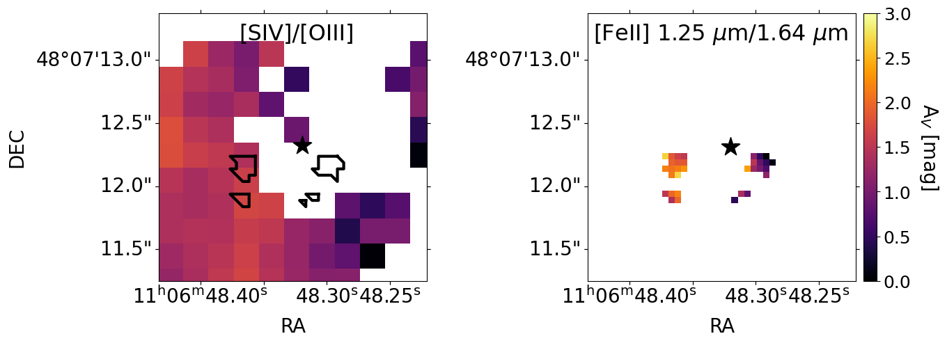
Figure 5: (left) Visual extinction A_V derived from the [O III]/[SIV] ratio, as presented in Rupke et al. (2023b), overlaid with an outline (in black) of the [Fe II] 1.2570/1.6440 µm extinction map distribution. (right) A_V map from the [Fe II] 1.2570/1.6440 µm ratio.

We determine the extinction by analyzing the relative flux between [Fe II] lines at 1.2570 and 1.6440 µm, both originating from the same upper state (a⁴D_7/2) (Antoniucci et al., 2014; Erkal et al., 2021). This ensures that their intrinsic ratio is governed solely by their respective Einstein A coefficients and wavelengths, specifically: $(I_{1.25}/I_{1.64})_{0}$$=$ (A_ki,1.26/A_ki,1.64)/(1.26/1.64). Previous studies (Cardelli et al., 1989; Giannini et al., 2015; Koo & Lee, 2015), have determined this ratio theoretically and observationally, reporting values ranging from 0.94 to 1.49. For our calculations, we adopt the more commonly quoted theoretical ratio of $(I_{1.25}/I_{1.64})_{0}$$=$ 1.36 from Cardelli et al. (1989). Extinction is then determined using the following formula, where E_B-V $=$ 0.3 $\times$ E_J-H (Draine, 1989) and A_V $=$ 3.1 $\times$ E_B-V:

$$I_{1.25}/I_{1.64}=(I_{1.25}/I_{1.64})_{0}\times 10^{-(E_{J-H})/2.5}.$$ (1)

The [Fe II] extinction (A_V) map is shown in Figure 5. Here, only spaxels with emission of both [Fe II] 1.2570 and 1.6440 µm larger than 3$\sigma$ are included, with the measurements mostly confined to the southwest and southeast of the quasar. For comparison, Figure 5 also shows the A_V map from Rupke et al. (2023b), where dust extinction is estimated by comparing the observed [SIV]/[O III] line ratios. Similarly to their result, we find that the southeast [Fe II] clump experiences higher extinction (median A_V$\sim$2.5 from the [Fe II] and A_V$\sim$2.0 from [SIV]/[O III] map) in comparison to the southwest one, where the extinction is relatively low (median A_V$\sim$0.1 from the [Fe II] and A_V$\sim$0.3 in [SIV]/[O III]). Rupke et al. (2023b) attribute their observations to the bipolar outflow model, where the redshifted region experiences greater dust attenuation due to obscuration by the host galaxy, while the blueshifted region is less obscured and shows less attenuation.

While both datasets qualitatively suggest higher extinction of the redshifted side, the specific measured values of A_V differ somewhat. This is due to significant uncertainties, as both methods use intrinsic ratios that vary in the literature. Additionally, the extinction derived from [Fe II] experiences systematic errors due to the differing velocity dispersions between the two lines. In our extinction measurements, we have not kinematically tied [Fe II] 1.2570 and 1.6440 µm fits, and therefore if the [Fe II] 1.2570µm velocity width is under-estimated because of its low SNR as discussed in Sec. 3.2, then its flux is under-estimated and the extinction is under-estimated. The [SIV]/[O III] extinction measure faces uncertainties from the depletion fraction of sulfur. Furthermore, [Fe II] and [SIV]/[O III] have different ionization energies (7.87 eV for [Fe II] and 35.1 eV for [SIV] and [O III]) and thus trace different gas phases.

3.5 Physical Conditions

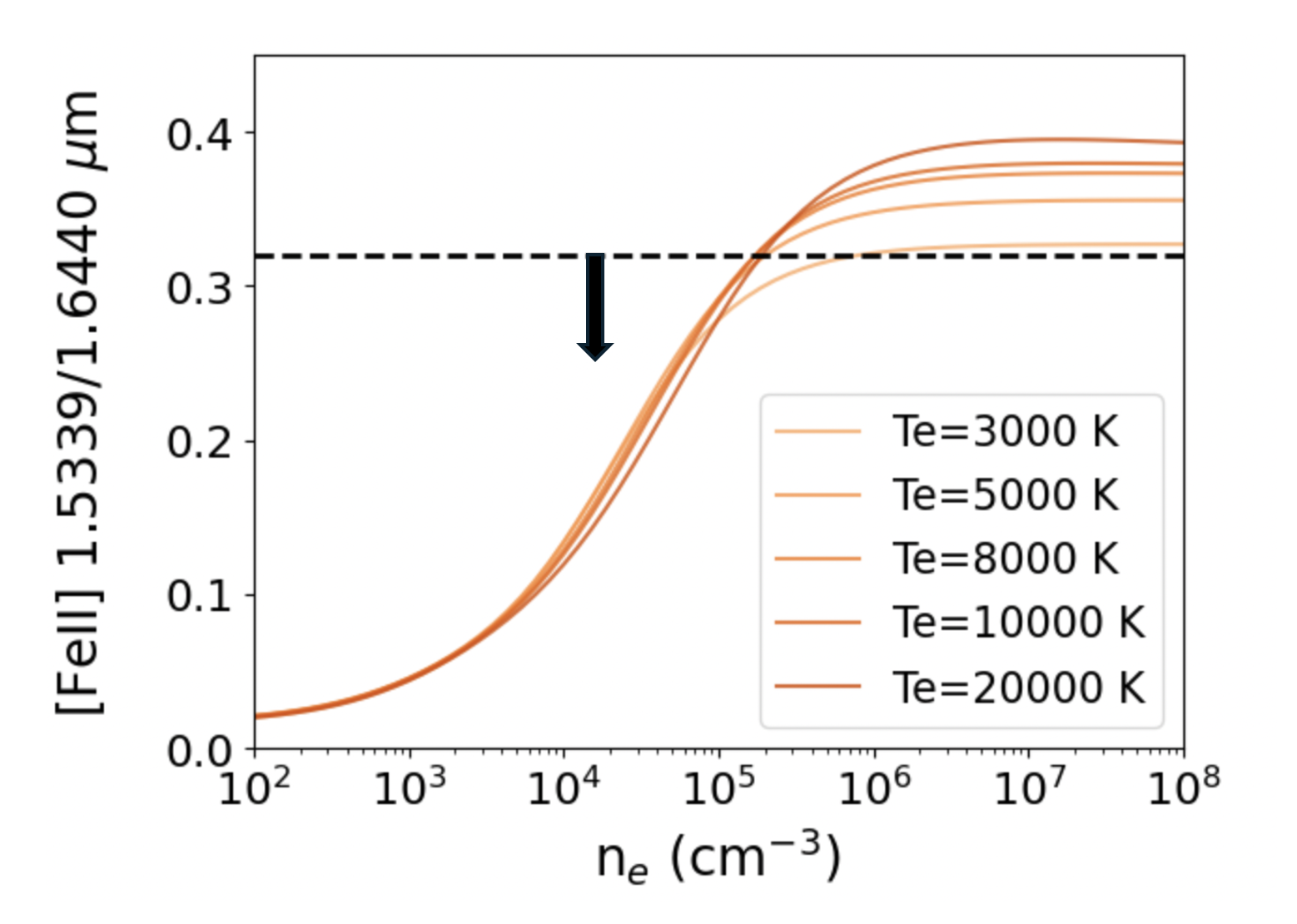
Figure 6: The figure shows the model [Fe II] emission-line ratios versus electron density for the ratio [FeII] 1.5339/1.6440 $\mu$m. Each sequence of models correspond to a different temperature – from bottom to top – 3, 5, 10 and 2 x 10³ K. We compute a 3$\sigma$ upper limit for the ratio in spaxels containing [Fe II] 1.6440 µm. The average value of the ratio is taken as an upper limit for the density, which is determined to be n_e$<$10^5.3cm^-3.

To determine the electron density of the [Fe II] emission, we utilize the density diagnostic [Fe II] 1.5339/1.6440 µm line ratio. Given that the [Fe II] 1.5339 µm line is not detected in our spectra, we establish a 3$\sigma$ upper limit on its flux while calculating the average [Fe II] 1.5339/1.6440 µm ratio for spaxels containing [Fe II] 1.6440 µm emission. Employing the PyNeb package (Luridiana et al., 2015), we compute electron densities for temperatures ranging from 3000 K to 20000 K, as depicted in Figure 6. Our analysis yields an upper limit on the electron density of n${}_{e}<$10^5.3 cm^-3. Studies using [Fe II] density diagnostics typically report such high densities, as the critical density for [Fe II] ranges from 10⁴ to 10^5.5 cm^-3, making [Fe II] a tracer for regions that are typically somewhat denser than those traced by [O III]. Specifically, Storchi-Bergmann et al. (2009) measure densities ranging from 10⁴ to 10⁵ cm^-3 in the nuclear region of NGC 4151 using the [Fe II] 1.5339/1.6440 µm line ratio, tapering off to 10³ cm^-3 beyond the central 0.5”. Similarly, Mazzalay & Rodríguez-Ardila (2007) find n${}_{e}\sim$10^5.2 cm^-3 for the nuclear region in Mrk 1210.

4 Discussion

4.1 Role of Radio Jets in [Fe II] Ionization

Figure 7: Radio luminosity at 1.4 GHz versus the velocity width W₉₀ of the [O III] emission for a radio-quiet sample, adapted from Hwang et al. (2018). The blue dots denote low-redshift (z $<$ 0.8) type 2 quasars from Zakamska & Greene (2014), with radio luminosity upper limits around 5$\sigma$ from FIRST and NVSS. The red triangles represent data from Zakamska et al. (2016b), and the orange squares are from Perrotta et al. (2019), both depicting an extremely red quasar population, with [O III] observations at redshifts near z$\sim$3, with radio luminosity upper limits of 4$\sigma$. The black line illustrates the quadratic fit derived solely from the low-redshift radio-quiet sample (blue dots), with the shaded region indicating the root-mean-square scatter. Open symbols mark candidate radio-loud sources. F2M1106 (this study) is shown as a green circle.

Our target is radio-quiet and point-like in the radio, with a steep radio spectrum ($\alpha$ $=$ -0.88). Typically, radio emission in active galactic nuclei is associated with processes such as jet activity. However, Zakamska & Greene (2014) study outflow velocites and radio luminosities of 568 obscured luminous quasars and find them to be strongly correlated in radio-quiet sources within their sample. The scenario they propose suggests that the radio emission observed in radio-quiet quasars is due to relativistic particles accelerated in the shocks within the quasar-driven outflows. More recently, Hwang et al. (2018) find the radio luminosity of their sample, which consists of 108 extremely red quasars at redshifts $z=2–4$, to be related to the velocity dispersion of the [O III]emitting ionized gas, drawing similar conclusions.

We take the highest velocity dispersion W₉₀ value for the [O III] as an upper limit and place F2M1106 on the radio luminosity vs [O III] relation in Figure 7 (Hwang et al., 2018). F2M1106 lies close to the [O III]-radio emission correlation of radio-quiet quasars. We find no evidence for a powerful radio jet in F2M1106, and therefore the observed [Fe II] is unlikely to be jet-excited. While there could still be a small nuclear jet in the object, it is unlikely to be responsible for the [Fe II] clumps.

4.2 Supernovae-Driven Shock Ionization

In Figure 4, we demonstrate that the kinematics of [Fe II] and [O III] are largely consistent with each other. Therefore, most of [Fe II] is embedded in the quasar-driven outflow, with the possible exception of the southern clump of [Fe II] which shows very low velocity dispersion compared to the values seen in [O III]. Here we examine whether supernova-driven shocks in the host galaxy would be sufficient to reproduce any of the observed [Fe II] fluxes.

To calculate the supernova rate required to produce the observed [Fe II] emission, we use the empirical relationship between the supernovae (SN) rate and [Fe II] 1.2570 µm line for starburst galaxies derived by Rosenberg et al. (2012):

$$\log\frac{\nu_{SNrate,\hbox{[Fe$\,${\scriptsize II}]}_{1.26}\micron}}{\rm{yr}^{-1}}=$$ (2)

$$(1.01\pm 0.2)\log\frac{L(\hbox{[Fe$\,${\scriptsize II}]}_{1.26\micron})}{\mbox{erg s}^{-1}}-(41.17\pm 0.9)$$

.

Due to the poor signal-to-noise ratio of the [Fe II] 1.2570 µm line in our observations and its nondetection to the south of the quasar, we use the [Fe II] 1.6440 µm line for our analysis instead, accounting for extinction where applicable. We select three apertures centered on spaxels A, B, and C, with diameters of 4.3”, 2.6”, and 2.5”, respectively, and determine the average extinction-corrected [Fe II] 1.6440 µm flux per aperture. The integrated luminosities of [Fe II] 1.6440 µm in each aperture are 5.5 $\times$ 10⁴¹ erg s^-1, 3.7 $\times$ 10⁴⁰ erg s^-1, and 5.9 $\times$ 10⁴⁰ erg s^-1 respectively. Using these values in equation 2, we compute integrated SN rates of $\nu_{\text{SNrate, \hbox{[Fe$\,${\scriptsize II}]}}}\sim$10, 0.6, and 0.9 yr^-1 per aperture. The star formation rate upper limit estimated in Section 2.2 of $\sim$132 M_⊙ yr^-1 corresponds to the supernova rate $\sim$2.2 yr^-1 (Kennicutt, 1998), assuming the Salpeter initial mass function in the mass range of 0.1–100 M_⊙ and solar metallicity. Therefore, the observed [Fe II] emission of aperture A cannot be explained by star formation alone and requires additional sources of ionization. While the supernova rate from star formation alone exceeds the rate required to produce the [Fe II] emission in apertures B and C, all of the star formation would have to be concentrated in these clumps to explain their [Fe II] emission. Additionally, given there is a wide range of galaxy templates that are in principle consistent with the SED in Section 2.2, the star formation rate estimate itself should be taken as approximate.

4.3 MAPPINGS III Shock Models

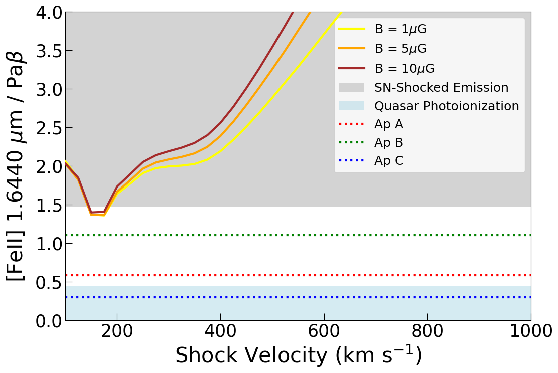
Figure 8: MAPPINGS III shock diagnostics using the kinematic components of [Fe II] 1.6440 µm and narrow Pa$\beta$ from fitting. The shock+precursor models are taken from Allen et al. (2008) for an electron density of 100 cm^-3and a solar metallicity. We allow the magnetic field to vary between values of 1, 5, and 10 $\mu$G cm^3/2. Additional line ratio ranges expected from pure supernovae-shock ionization and pure photoionization are indicated in light gray and light blue respectively (Rodríguez-Ardila et al., 2004). We plot the average line ratios taken from previously defined apertures A, B, and C in red, green, and blue respectively.

We use MAPPINGS III (Allen et al., 2008) models to determine the source of ionization of [Fe II]. These models are particularly relevant for fast shocks, where the ionizing radiation arises from the cooling of hot gas heated by shocks. This process generates a substantial field of extreme ultraviolet and soft X-ray photons, accounting for ionization from both quasar outflow-driven shocks and supernovae-driven shocks. The models include the following parameters: shock velocity (ranging from 100 to 1000 km s^-1 in increments of 25 km s^-1), preshock density (ranging from 10^-2 to 10³ cm^-3 in logarithmic steps of 10), and preshock transverse magnetic field strength (ranging from 10^-4 to 10³ $\mu G$).

The [Fe II] 1.2570 µm/Pa$\beta$ line ratio is a well-established diagnostic for shocked emission. This ratio typically falls below 0.6 in starbursts, but rises above 2.0 in regions where shocks driven by supernovae are the primary mechanism (Rodríguez-Ardila et al., 2004). In active galaxies, the ratio generally ranges between 0.6 and 2.0, with values near 0.6 indicating photoionization (either from the active galactic nuclei or ongoing star formation) as the prevailing process, while values approaching or exceeding 2.0 suggest a greater contribution from shock excitation, particularly supernovae-driven (Mouri et al., 2000; Rodríguez-Ardila et al., 2004; Riffel et al., 2008; Storchi-Bergmann et al., 2009). However, due to the low signal-to-noise of [Fe II] 1.2570 µm, we instead use the [Fe II] 1.6440 µm/Pa$\beta$ line ratio.

Figure 8 presents the mean integrated, extinction-corrected [Fe II]1.6440 µm/Pa$\beta$ line ratios for apertures A, B, and C. We compare these values to the shock models, which are insensitive to changes in electron density. Therefore, we fix the electron density at 1000 cm^-3 and assume solar metallicity for our radiative shock and precursor models. We allow the magnetic field strength to vary from 1, 5, and 10 $\mu$G cm^3/2. Additionally, we highlight line ratio ranges expected for pure supernova shock excitation and purely photoionized regions, converted to [Fe II] 1.6440 µm/Pa$\beta$ ratios using an intrinsic line flux ratio of $(I_{1.25}/I_{1.64})_{0}=1.36$ (Cardelli et al., 1989).

Our observations reveal that the average line ratios for all three apertures in each case are consistently lower than both the shock models and the range of line ratios expected from purely supernovae-shock ionized emission. From Figure 8, we find the excitation mechanism in aperture C, previously concluded to be within the outflow in Section 3.3, to be largely photoionized (similarly concluded by (Rupke et al., 2023b) using mid-infrared [SIV]).

In contrast, the higher average line ratio in apertures A and B suggest partial shock ionization. While the models themselves cannot differentiate between shock ionization due to star formation processes and that due to quasar outflows, we have previously demonstrated that, while star formation is in principle sufficient to generate the [Fe II] emission in clump B, it would have to be strongly concentrated in this one clump. We also concluded that the [Fe II] emission in aperture A requires additional sources of ionization aside from star formation. Given that F2M1106 has an extraordinarily fast and extended [O III] outflow, we instead explore the possibility that the shock ionization in both clumps is due to quasar winds instead.

In particular, our analysis places [Fe II] emission in aperture B within the host galaxy, both spatially and kinematically (the velocity centroid and the velocity dispersion of [Fe II] in this aperture are strongly inconsistent with those of [O III]). Given that galactic outflows are strongly influenced by the distribution and clumping of the interstellar medium, and these winds can hydrodynamically navigate around dense obstacles (Wagner et al., 2013), it is possible that we are observing the outflow in this object reaching parts of the galaxy not directly illuminated by the quasar and proceeding to ionize them. Furthermore, theoretical studies indicate that wide-angle outflows can exert pressure greater than the maximum gas pressure in the host galaxy, compressing cold gas and potentially triggering star formation (King et al., 2011; Nayakshin & Zubovas, 2012). This compression may also be potentially responsible for inducing shocks and producing the [Fe II] in this region.

We analyze the data initially using the non-PSF-subtracted Pa$\beta$ map. However, the broad component detected near the quasar, with a velocity of v${}_{50}\sim$ 3000 km s^-1, could potentially contaminate our extended Pa$\beta$ measurements in regions with [Fe II] and overall artificially lower the measures ratios. To address this, we PSF subtract the Pa$\beta$ line and remeasure the average line ratios in apertures A, B, and C. This adjustment increases the ratios to 1.0, 1.2, and 1.9, respectively, suggesting a greater contribution of shocks in all three apertures, which would have to be largely due to the quasar winds since the total amount of [Fe II] emission in clumps A, B and C is inconsistent with star formation. However, given the risk of oversubtraction, we interpret these results with caution.

5 Summary

In this paper, we examine the ionizing mechanism of [Fe II] emission in JWST NIRSpec IFU data of F2M1106, a red quasar at $z=0.4352$ with a known powerful outflow in [O III]. Our results are summarized as follows:

• We model the spectral energy distribution (SED) of the object across optical to far-infrared wavelengths, incorporating data from GALEX, SDSS, 2MASS, WISE, and SOFIA. The SED reveals a continuum extinction of A${}_{V}\sim$ 3.2 mag and a bolometric luminosity of L_bol $=$ 10^46.5±0.1 erg s^-1. Analysis of the broad H$\alpha$ emission line indicates a black hole mass of M_BH $\sim$ 10^9.5±0.2 M_⊙ and an Eddington ratio of log log$\lambda_{Edd}$ $\sim$ –1.0 $\pm$ 0.3.

• Analysis of the the NIRSpec IFU data reveals evidence of [Fe II] lines at 1.2570, 1.2791, and 1.6440 µm and Pa$\beta$. All three [Fe II] lines are clumpy, but not necessarily cospatial ([Fe II] 1.2570 µm is not detected in the southern region due to poor SNR; [Fe II] 1.2791 µm is blended with Pa$\beta$ in the southwest). The Pa$\beta$ map shows broad-line emission near the quasar, with narrower lines in regions where [Fe II] is present.

• We analyze the extinction in F2M1106 using the [Fe II] 1.2570/1.6440 µm line ratio, revealing higher extinction in the redshifted southeast region (A${}_{V}\sim$ 2.5) compared to the blueshifted southwest (A${}_{V}\sim$ 0.1). This is consistent with previous [SIV]/[O III] findings, but shows some variance due to method-specific uncertainties. The electron density is constrained using the [Fe II] 1.5339/1.6440 µm line ratio, with an upper limit of n_e $<$ 10^5.3 cm^-3, indicating that the [Fe II]-emitting regions are associated with dense gas.

• Two of the three clumps of the [Fe II] 1.6440 µm emission are kinematically consistent with the outflow traced by [O III]$\lambda$5007 Å. Both lines show two major velocity components: a redshifted nebula in the southeast (with [Fe II] v₅₀ $\sim$50–1100 km s^-1) and a blueshifted nebula in the southwest ([Fe II] v₅₀ $\sim$–1200–0 km s^-1), both with high velocity widths. These velocities, exceeding typical galaxy rotation speeds, align with the [O III] outflow. In contrast, the [Fe II] emission in the southern region shows narrower velocity widths (W₈₀ $\sim$460 km s^-1) compared to [O III] (W₈₀ $\sim$1630 km s^-1), suggesting that part of the [Fe II] emission in the south may be located within the host galaxy.

• Using MAPPINGS III models, we find that the [Fe II]/Pa$\beta$ line ratios indicate quasar photoionization as the primary ionization mechanism for [Fe II] in apertures A (southeast [Fe II] emitting region) and C (southwest). The higher ratio in aperture B (the south region) suggests partial shock ionization. We suggest that this region experiences increased back pressure from the quasar-driven outflow which exceeds the maximum host galaxy pressure and compresses the gas, inducing shocks.

6 Appendix

Table 2: F2M1106 Photometry

Band	Wavelength ($\mu$m)	AB Mag
GALEX NUV	0.231	20.40 $\pm$ 0.06
SDSS u	0.355	19.81 $\pm$ 0.06
SDSS g	0.468	19.01 $\pm$ 0.03
SDSS r	0.616	18.25 $\pm$ 0.03
SDSS i	0.748	17.70 $\pm$ 0.03
SDSS z	0.893	17.37 $\pm$ 0.03
2MASS J	1.235	17.16 $\pm$ 0.10
2MASS H	1.662	16.51 $\pm$ 0.09
2MASS K	2.159	15.79 $\pm$ 0.06
WISE W1	3.352	14.34 $\pm$ 0.04
WISE W2	4.602	13.67 $\pm$ 0.04
WISE W3	11.560	12.78 $\pm$ 0.03
WISE W4	22.090	12.09 $\pm$ 0.04
SOFIA HAWC+ C	62	$<$ 14.89
SOFIA HAWC+ D	107	$<$ 14.65

References

- Allen et al. (1999) Allen, M. G., Dopita, M. A., Tsvetanov, Z. I., & Sutherland, R. S. 1999, ApJ, 511, 686, doi: 10.1086/306718
- Allen et al. (2008) Allen, M. G., Groves, B. A., Dopita, M. A., Sutherland, R. S., & Kewley, L. J. 2008, ApJS, 178, 20, doi: 10.1086/589652
- Antoniucci et al. (2014) Antoniucci, S., Arkharov, A. A., Di Paola, A., et al. 2014, A&A, 565, L7, doi: 10.1051/0004-6361/201423962
- Banerji et al. (2015) Banerji, M., Alaghband-Zadeh, S., Hewett, P. C., & McMahon, R. G. 2015, MNRAS, 447, 3368, doi: 10.1093/mnras/stu2649
- Bell (2003) Bell, E. F. 2003, ApJ, 586, 794, doi: 10.1086/367829
- Bennett et al. (2014) Bennett, C. L., Larson, D., Weiland, J. L., & Hinshaw, G. 2014, ApJ, 794, 135, doi: 10.1088/0004-637X/794/2/135
- Bertemes et al. (2024) Bertemes, C., Wylezalek, D., Rupke, D. S. N., et al. 2024, arXiv e-prints, arXiv:2404.14475, doi: 10.48550/arXiv.2404.14475
- Boroson & Green (1992) Boroson, T. A., & Green, R. F. 1992, ApJS, 80, 109, doi: 10.1086/191661
- Cardelli et al. (1989) Cardelli, J. A., Clayton, G. C., & Mathis, J. S. 1989, ApJ, 345, 245, doi: 10.1086/167900
- Dopita et al. (2003) Dopita, M. A., Groves, B. A., Sutherland, R. S., & Kewley, L. J. 2003, ApJ, 583, 727, doi: 10.1086/345448
- Draine (1989) Draine, B. T. 1989, in Infrared Spectroscopy in Astronomy, ed. E. Böhm-Vitense, 93
- Eisenstein et al. (2011) Eisenstein, D. J., Weinberg, D. H., Agol, E., et al. 2011, AJ, 142, 72, doi: 10.1088/0004-6256/142/3/72
- Erkal et al. (2021) Erkal, J., Nisini, B., Coffey, D., et al. 2021, ApJ, 919, 23, doi: 10.3847/1538-4357/ac06c5
- Fabian (2012) Fabian, A. C. 2012, ARA&A, 50, 455, doi: 10.1146/annurev-astro-081811-125521
- Fawcett et al. (2023) Fawcett, V. A., Alexander, D. M., Brodzeller, A., et al. 2023, MNRAS, 525, 5575, doi: 10.1093/mnras/stad2603
- Giannini et al. (2015) Giannini, T., Antoniucci, S., Nisini, B., et al. 2015, ApJ, 798, 33, doi: 10.1088/0004-637X/798/1/33
- Glikman et al. (2007) Glikman, E., Helfand, D. J., White, R. L., et al. 2007, ApJ, 667, 673, doi: 10.1086/521073
- Glikman et al. (2017) Glikman, E., LaMassa, S., Piconcelli, E., Urry, M., & Lacy, M. 2017, ApJ, 847, 116, doi: 10.3847/1538-4357/aa88ac
- Glikman et al. (2024) Glikman, E., LaMassa, S., Piconcelli, E., Zappacosta, L., & Lacy, M. 2024, MNRAS, 528, 711, doi: 10.1093/mnras/stae042
- Glikman et al. (2012) Glikman, E., Urrutia, T., Lacy, M., et al. 2012, ApJ, 757, 51, doi: 10.1088/0004-637X/757/1/51
- Glikman et al. (2022) Glikman, E., Lacy, M., LaMassa, S., et al. 2022, ApJ, 934, 119, doi: 10.3847/1538-4357/ac6bee
- Graham et al. (1987) Graham, J. R., Wright, G. S., & Longmore, A. J. 1987, ApJ, 313, 847, doi: 10.1086/165023
- Greene et al. (2014) Greene, J. E., Pooley, D., Zakamska, N. L., Comerford, J. M., & Sun, A.-L. 2014, ApJ, 788, 54, doi: 10.1088/0004-637X/788/1/54
- Greene et al. (2012) Greene, J. E., Zakamska, N. L., & Smith, P. S. 2012, ApJ, 746, 86, doi: 10.1088/0004-637X/746/1/86
- Greene et al. (2024) Greene, J. E., Labbe, I., Goulding, A. D., et al. 2024, ApJ, 964, 39, doi: 10.3847/1538-4357/ad1e5f
- Guo et al. (2018) Guo, H., Shen, Y., & Wang, S. 2018, PyQSOFit: Python code to fit the spectrum of quasars, Astrophysics Source Code Library, record ascl:1809.008. http://ascl.net/1809.008
- Harper et al. (2018) Harper, D. A., Runyan, M. C., Dowell, C. D., et al. 2018, Journal of Astronomical Instrumentation, 7, 1840008, doi: 10.1142/S2251171718400081
- Harrison et al. (2014) Harrison, C. M., Alexander, D. M., Mullaney, J. R., & Swinbank, A. M. 2014, MNRAS, 441, 3306, doi: 10.1093/mnras/stu515
- Hu et al. (2008) Hu, C., Wang, J.-M., Ho, L. C., et al. 2008, ApJ, 687, 78, doi: 10.1086/591838
- Hwang et al. (2018) Hwang, H.-C., Zakamska, N. L., Alexandroff, R. M., et al. 2018, MNRAS, 477, 830, doi: 10.1093/mnras/sty742
- Ishikawa et al. (2021) Ishikawa, Y., Goulding, A. D., Zakamska, N. L., et al. 2021, MNRAS, 502, 3769, doi: 10.1093/mnras/stab137
- Jahnke et al. (2004) Jahnke, K., Sánchez, S. F., Wisotzki, L., et al. 2004, ApJ, 614, 568, doi: 10.1086/423233
- Jakobsen et al. (2022) Jakobsen, P., Ferruit, P., Alves de Oliveira, C., et al. 2022, A&A, 661, A80, doi: 10.1051/0004-6361/202142663
- Kennicutt (1998) Kennicutt, Jr., R. C. 1998, ARA&A, 36, 189, doi: 10.1146/annurev.astro.36.1.189
- Kim et al. (2006) Kim, M., Ho, L. C., & Im, M. 2006, ApJ, 642, 702, doi: 10.1086/501422
- King (2003) King, A. 2003, ApJ, 596, L27, doi: 10.1086/379143
- King & Pounds (2015) King, A., & Pounds, K. 2015, ARA&A, 53, 115, doi: 10.1146/annurev-astro-082214-122316
- King et al. (2011) King, A. R., Zubovas, K., & Power, C. 2011, MNRAS, 415, L6, doi: 10.1111/j.1745-3933.2011.01067.x
- Koo & Lee (2015) Koo, B.-C., & Lee, Y.-H. 2015, Publication of Korean Astronomical Society, 30, 145, doi: 10.5303/PKAS.2015.30.2.145
- Koo et al. (2007) Koo, B.-C., Moon, D.-S., Lee, H.-G., Lee, J.-J., & Matthews, K. 2007, ApJ, 657, 308, doi: 10.1086/510550
- Kormendy & Ho (2013) Kormendy, J., & Ho, L. C. 2013, ARA&A, 51, 511, doi: 10.1146/annurev-astro-082708-101811
- Lacy et al. (2017) Lacy, M., Croft, S., Fragile, C., Wood, S., & Nyland, K. 2017, ApJ, 838, 146, doi: 10.3847/1538-4357/aa65d7
- LaMassa et al. (2016) LaMassa, S. M., Ricarte, A., Glikman, E., et al. 2016, ApJ, 820, 70, doi: 10.3847/0004-637X/820/1/70
- Lee et al. (2009) Lee, H.-G., Moon, D.-S., Koo, B.-C., Lee, J.-J., & Matthews, K. 2009, ApJ, 691, 1042, doi: 10.1088/0004-637X/691/2/1042
- Leung et al. (2021) Leung, G. C. K., Coil, A. L., Rupke, D. S. N., & Perrotta, S. 2021, ApJ, 914, 17, doi: 10.3847/1538-4357/abf4da
- Liu et al. (2013) Liu, G., Zakamska, N. L., Greene, J. E., Nesvadba, N. P. H., & Liu, X. 2013, MNRAS, 436, 2576, doi: 10.1093/mnras/stt1755
- Liu et al. (2024) Liu, W., Veilleux, S., Sankar, S., et al. 2024, arXiv e-prints, arXiv:2410.14291, doi: 10.48550/arXiv.2410.14291
- Luridiana et al. (2015) Luridiana, V., Morisset, C., & Shaw, R. A. 2015, A&A, 573, A42, doi: 10.1051/0004-6361/201323152
- MacArthur et al. (2004) MacArthur, L. A., Courteau, S., Bell, E., & Holtzman, J. A. 2004, ApJS, 152, 175, doi: 10.1086/383525
- Martin et al. (2005) Martin, D. C., Fanson, J., Schiminovich, D., et al. 2005, ApJ, 619, L1, doi: 10.1086/426387
- Mazzalay & Rodríguez-Ardila (2007) Mazzalay, X., & Rodríguez-Ardila, A. 2007, A&A, 463, 445, doi: 10.1051/0004-6361:20054194
- Mouri et al. (2000) Mouri, H., Kawara, K., & Taniguchi, Y. 2000, ApJ, 528, 186, doi: 10.1086/308142
- Mukherjee et al. (2016) Mukherjee, D., Bicknell, G. V., Sutherland, R., & Wagner, A. 2016, MNRAS, 461, 967, doi: 10.1093/mnras/stw1368
- Nayakshin & Zubovas (2012) Nayakshin, S., & Zubovas, K. 2012, MNRAS, 427, 372, doi: 10.1111/j.1365-2966.2012.21950.x
- Obied et al. (2016) Obied, G., Zakamska, N. L., Wylezalek, D., & Liu, G. 2016, MNRAS, 456, 2861, doi: 10.1093/mnras/stv2850
- Oliva et al. (1989) Oliva, E., Moorwood, A. F. M., & Danziger, I. J. 1989, A&A, 214, 307
- Perrotta et al. (2019) Perrotta, S., Hamann, F., Zakamska, N. L., et al. 2019, MNRAS, 488, 4126, doi: 10.1093/mnras/stz1993
- Peterson et al. (2004) Peterson, B. M., Ferrarese, L., Gilbert, K. M., et al. 2004, ApJ, 613, 682, doi: 10.1086/423269
- Polletta et al. (2007) Polletta, M., Tajer, M., Maraschi, L., et al. 2007, ApJ, 663, 81, doi: 10.1086/518113
- Reach et al. (2005) Reach, W. T., Rho, J., & Jarrett, T. H. 2005, ApJ, 618, 297, doi: 10.1086/425855
- Reach et al. (2002) Reach, W. T., Rho, J., Jarrett, T. H., & Lagage, P.-O. 2002, ApJ, 564, 302, doi: 10.1086/324075
- Reunanen et al. (2002) Reunanen, J., Kotilainen, J. K., & Prieto, M. A. 2002, MNRAS, 331, 154, doi: 10.1046/j.1365-8711.2002.05181.x
- Reunanen et al. (2003) —. 2003, MNRAS, 343, 192, doi: 10.1046/j.1365-8711.2003.06771.x
- Richards et al. (2006) Richards, G. T., Lacy, M., Storrie-Lombardi, L. J., et al. 2006, ApJS, 166, 470, doi: 10.1086/506525
- Riffel et al. (2021a) Riffel, R., Mallmann, N. D., Ilha, G. S., et al. 2021a, MNRAS, 501, 4064, doi: 10.1093/mnras/staa3907
- Riffel et al. (2008) Riffel, R. A., Storchi-Bergmann, T., Winge, C., et al. 2008, MNRAS, 385, 1129, doi: 10.1111/j.1365-2966.2008.12936.x
- Riffel et al. (2021b) Riffel, R. A., Dors, O. L., Armah, M., et al. 2021b, MNRAS, 501, L54, doi: 10.1093/mnrasl/slaa194
- Rodríguez-Ardila et al. (2004) Rodríguez-Ardila, A., Pastoriza, M. G., Viegas, S., Sigut, T. A. A., & Pradhan, A. K. 2004, A&A, 425, 457, doi: 10.1051/0004-6361:20034285
- Rosenberg et al. (2012) Rosenberg, M. J. F., van der Werf, P. P., & Israel, F. P. 2012, A&A, 540, A116, doi: 10.1051/0004-6361/201218772
- Rupke et al. (2023a) Rupke, D., Wylezalek, D., Zakamska, N., et al. 2023a, q3dfit: PSF decomposition and spectral analysis for JWST-IFU spectroscopy, Astrophysics Source Code Library, record ascl:2310.004
- Rupke (2014) Rupke, D. S. N. 2014, IFSFIT: Spectral Fitting for Integral Field Spectrographs. http://ascl.net/1409.005
- Rupke et al. (2017) Rupke, D. S. N., Gültekin, K., & Veilleux, S. 2017, ApJ, 850, 40, doi: 10.3847/1538-4357/aa94d1
- Rupke et al. (2023b) Rupke, D. S. N., Wylezalek, D., Zakamska, N. L., et al. 2023b, ApJ, 953, L26, doi: 10.3847/2041-8213/aced85
- Shen et al. (2023) Shen, L., Liu, G., He, Z., et al. 2023, Science Advances, 9, eadg8287, doi: 10.1126/sciadv.adg8287
- Shen & Liu (2012) Shen, Y., & Liu, X. 2012, ApJ, 753, 125, doi: 10.1088/0004-637X/753/2/125
- Shimwell et al. (2017) Shimwell, T. W., Röttgering, H. J. A., Best, P. N., et al. 2017, A&A, 598, A104, doi: 10.1051/0004-6361/201629313
- Silk & Rees (1998) Silk, J., & Rees, M. J. 1998, A&A, 331, L1
- Skrutskie et al. (2006) Skrutskie, M. F., Cutri, R. M., Stiening, R., et al. 2006, AJ, 131, 1163, doi: 10.1086/498708
- Storchi-Bergmann et al. (2009) Storchi-Bergmann, T., McGregor, P. J., Riffel, R. A., et al. 2009, MNRAS, 394, 1148, doi: 10.1111/j.1365-2966.2009.14388.x
- Urrutia et al. (2008) Urrutia, T., Lacy, M., & Becker, R. H. 2008, ApJ, 674, 80, doi: 10.1086/523959
- Urrutia et al. (2012) Urrutia, T., Lacy, M., Spoon, H., et al. 2012, ApJ, 757, 125, doi: 10.1088/0004-637X/757/2/125
- Vanden Berk et al. (2001) Vanden Berk, D. E., Richards, G. T., Bauer, A., et al. 2001, AJ, 122, 549, doi: 10.1086/321167
- Vayner et al. (2023) Vayner, A., Zakamska, N. L., Ishikawa, Y., et al. 2023, ApJ, 955, 92, doi: 10.3847/1538-4357/ace784
- Veilleux et al. (2020) Veilleux, S., Maiolino, R., Bolatto, A. D., & Aalto, S. 2020, A&A Rev., 28, 2, doi: 10.1007/s00159-019-0121-9
- Veilleux et al. (2023) Veilleux, S., Liu, W., Vayner, A., et al. 2023, ApJ, 953, 56, doi: 10.3847/1538-4357/ace10f
- Wagner et al. (2016) Wagner, A. Y., Bicknell, G. V., Umemura, M., Sutherland, R. S., & Silk, J. 2016, Astronomische Nachrichten, 337, 167, doi: 10.1002/asna.201512287
- Wagner et al. (2013) Wagner, A. Y., Umemura, M., & Bicknell, G. V. 2013, ApJ, 763, L18, doi: 10.1088/2041-8205/763/1/L18
- Weingartner & Draine (2001) Weingartner, J. C., & Draine, B. T. 2001, ApJ, 548, 296, doi: 10.1086/318651
- White et al. (1997) White, R. L., Becker, R. H., Helfand, D. J., & Gregg, M. D. 1997, ApJ, 475, 479, doi: 10.1086/303564
- Wright et al. (2010) Wright, E. L., Eisenhardt, P. R. M., Mainzer, A. K., et al. 2010, AJ, 140, 1868, doi: 10.1088/0004-6256/140/6/1868
- Wylezalek et al. (2022) Wylezalek, D., Vayner, A., Rupke, D. S. N., et al. 2022, arXiv e-prints, arXiv:2210.10074. https://arxiv.org/abs/2210.10074
- Young et al. (2009) Young, S., Axon, D. J., Robinson, A., & Capetti, A. 2009, ApJ, 698, L121, doi: 10.1088/0004-637X/698/2/L121
- Zakamska & Greene (2014) Zakamska, N. L., & Greene, J. E. 2014, MNRAS, 442, 784, doi: 10.1093/mnras/stu842
- Zakamska et al. (2005) Zakamska, N. L., Schmidt, G. D., Smith, P. S., et al. 2005, AJ, 129, 1212, doi: 10.1086/427543
- Zakamska et al. (2006) Zakamska, N. L., Strauss, M. A., Krolik, J. H., et al. 2006, AJ, 132, 1496, doi: 10.1086/506986
- Zakamska et al. (2016a) Zakamska, N. L., Hamann, F., Pâris, I., et al. 2016a, MNRAS, 459, 3144, doi: 10.1093/mnras/stw718
- Zakamska et al. (2016b) Zakamska, N. L., Lampayan, K., Petric, A., et al. 2016b, MNRAS, 455, 4191, doi: 10.1093/mnras/stv2571
- Zovaro et al. (2019) Zovaro, H. R. M., Sharp, R., Nesvadba, N. P. H., et al. 2019, MNRAS, 484, 3393, doi: 10.1093/mnras/stz233