section [0pt] \thecontentslabel \contentspage \titlecontentssubsection [5pt] \thecontentslabel \contentspage \titlecontentssubsubsection [10pt] \thecontentslabel \contentspage \titlecontentsparagraph [15pt] \thecontentslabel \contentspage
The non-linear steepest descent approach to the singular asymptotics of the sinh-Gordon reduction of the Painlevé III equation
Abstract.
Motivated by the simplest case of tt*-Toda equations, we study the large and small asymptotics for of real solutions of the sinh-Godron Painlevé III() equation. These solutions are parametrized through the monodromy data of the corresponding Riemann-Hilbert problem. This unified approach provides connection formulae between the behavior at the origin and infinity of the considered solutions.
Keywords: Painlevé III equation; sinh-Gordon equation; isomonodromic deformation; Riemann-Hilbert problem; steepest-descent method
1 Introduction
The tt* (topological—anti-topological fusion) equations were introduced by Cecotti and Vafa to describe certain deformations of super-symmetric quantum field theories [CV91, CV92, CV93]. Our interest lies in the special case known as tt*-Toda equations subject to the anti-symmetry and radial symmetry conditions [GL14, GIL15a, GIL15b, GIL20]. In the simplest case (tt*-Toda equation of type ) it becomes
| (1.0.1) |
where , , and . It is well known that the above equation is a special reduction of the Painlevé III() equation, given, in the canonical form, by
| (1.0.2) |
where , and are some complex parameters such that . If we choose and , then any of the four functions solves (1.0.2) if is a solution of the sinh-Gordon Painlevé III equation
| (1.0.3) |
which is identical to (1.0.1) subject to a minor transformation . A further transformation brings (1.0.3) into the radial symmetric reduction of the elliptic sine-Gordon equation:
| (1.0.4) |
which is usually called the sine-Gordon Painlevé III equation and plays an important role in the study of the 2D Ising model [BMW73, MTW77].
Due to our interest in tt*-Toda equations, we study asymptotics (as and ) of real solutions of (1.0.3). More precisely, recall that solutions of (1.0.2) can have non-polar singularities only at and while polar singularities in do depend on the considered solution (this is the so-called Painlevé property). Hence, solutions of the sinh-Gordon reduction (1.0.3) of (1.0.2) can have movable logarithmic singularities. It also can be readily verified that solutions of (1.0.2) can only have simple poles. Thus, going around any logarithmic singularity (via the complex plane) of a solution of (1.0.3) will result in the addition of to this solution. So, when we speak of real solutions, we ignore all the acquired additions of (since (1.0.3) does not change when is replaced by , , thus obtained functions are still local solutions of (1.0.3)). Clearly, real solutions of (1.0.3) correspond to the real (on ) solutions of (1.0.2).
Investigations of this type are not new. A lot of information on the history of the sine/sinh-Gordon Painlevé III equation can be found in the monograph [FIKN06]. In particular, McCoy, Tracy, and Wu [MTW77] constructed a one-parameter family of solutions of (1.0.2) with that remain bounded for large and described their behavior as and . These solutions are in fact smooth on the whole and are called global solutions, see [GIL15b]. Later, Novokshënov [Nov86] asymptotically identified the locations of singularities of non-smooth real solutions of (1.0.3) parametrized by their behavior at the origin: for some .
A substantial amount of work has been dedicated to describing asymptotics of the solutions of (1.0.4) similarly parametrized by their behavior at the origin via
| (1.0.5) |
In [Nov84, Nov85], Novokshënov studied asymptotics as of the real solutions, which correspond to purely imaginary solutions of (1.0.3). In [Nov07, Nov08], assuming , , he described asymptotics of (1.0.5) for large , , in terms of the Jacobi function (when are purely imaginary, this provides asymptotics of the real solutions of (1.0.3) in the first quadrant). Asymptotics as of (1.0.5) for a range of parameters including purely imaginary ones with , can be found in the introduction of [IP16]. Even though these asymptotics can be obtained from the work of Kitaev [Kit87] outlined in the next paragraph, they were re-derived by the authors using the Riemann-Hilbert approach employed in this paper. Let us point out that the small asymptotics (1.0.5) does not describe all the behavior of solutions near , see Theorem 2.2 further below, which is based on the work of Niles [Nil09].
In [Kit87], Kitaev used the isomonodromy theory and the WKB method to find the connection formulae for the small and large parameter asymptotics of the solutions of the degenerate Painlevé V equation, which bijectively corresponds to Painlevé III(). These results then in principle allow one to extract the large and small asymptotics of the solutions of (1.0.3) via certain non-trivial changes of variables. However, these transformations are rather complicated. More importantly, the approach taken in [Kit87] does not readily generalize to tackling the asymptotics of tt*-Toda equations of type for general , which is our overarching goal. On the other hand, the approach we take here of parametrizing solutions via the monodromy data of the associated linear system and then applying Deift-Zhou steepest descent techniques [DZ93] as and techniques of Niles [Nil09] as to the corresponding Riemann-Hilbert problem seem to be much more promising in this regard, see [GIK+23].
2 Main Results
As standard in the theory of Painlevé transcendents, we parameterize the solutions by the monodromy data of the corresponding Riemann-Hilbert problem. Section 3 contains a detailed description of how this parameterization is achieved. At this point, it suffices to say that the monodromy data can be represented by a single parameter that belongs to , where is the open unit disk centered at the origin. Our main result is the following theorem.
Theorem 2.1.
To each finite , , there corresponds one real solution of the sinh-Gordon Painlevé III equation (1.0.3) on and
| (2.0.1) |
as , where the error term is uniform in ,
| (2.0.2) |
To there corresponds a one-parameter family of real solutions of the sinh-Gordon Painlevé III equation (1.0.3) on such that
| (2.0.3) |
as , where is the parametrizing (Stokes) parameter and is the modified Bessel function of the second kind.
Remark.
Recall, see [DLMF, Equation (10.40.2)], that for large it holds that
Remark.
Formula (2.0.1) implies that if we label the singularities of by in the increasing order, then for all natural numbers large enough it holds that
| (2.0.4) |
Remark.
Denote by the complement of in . Then,
where the error term is uniform on for all large (i.e., locally uniformly in ).
Remark.
As mentioned in the introduction, the location of poles of , the corresponding solution of (1.0.2), has been investigated in [Nov86] when . Novokshënov considered (1.0.3) with replaced with , in which case the solution is given by . Moreover, he was only interested in the singularities if that lead to the poles of (and not zeros), i.e., in . These points were denote by in [Nov86, Equation (0.9)] (this formula has a typo, needs to be replaced by as evident from [Nov86, Equations (1.1) and (4.9)]). Then one can readily verify that and have exactly the same asymptotic behavior upon noticing that in [Nov86, Equation (0.2)] are equal to , see Theorem 2.2 further below, and from [Nov86, Equation (0.8)] can be expressed as
Due to [Nil09], one can describe the asymptotic behavior near of the real solutions of (1.0.3) using the above parameter , which provides the connection formulae between asymptotics near infinity and the origin for each real solution.
Theorem 2.2.
When , the corresponding real solutions of the sinh-Gordon Painlevé III equation (1.0.3) parametrized by the Stokes parameter as in Theorem 2.1 admit the following asymptotic behavior on near the origin:
| (2.0.5) |
where the error terms hold as and, in the third case, it is locally uniform in the complement of (asymptotic locations of the singularities),
is the Euler’s constant, and
For finite , , the corresponding real solution of the sinh-Gordon Painlevé III equation (1.0.3) admits asymptotic behavior on near the origin as in (2.0.5), this time depending on the value of and with constants replaced by
where .
Remark.
Remark.
Theorems 2.1 and 2.2 provide a connection between the behavior at infinity and around the origin along of the corresponding solutions Painlevé III equation (1.0.2), but only up to a sign since and is defined up to addition of integer multiples of . However, the proofs of these theorems allow us to determine the sign uniquely, which we do in Appendix A.
Remark.
Recent paper [Li24, Section 4.1] conjectures, based on numerical analysis, singular asymptotics near the origin of exponentially decaying near infinity solutions of the tt*-Toda equation of type :
| (2.0.6) |
where are real-valued functions of on . Clearly, a further assumption reduces (2.0.6) to (1.0.1). Theorem 2.2 proves the conjecture in this degenerate case, see Appendix B for details.
As standard in the theory of Painlevé transcendents, we view (1.0.3) as a compatibility condition of an overdetermined system of linear differential equations, a Lax pair. A Lax pair for the sinh-Gordon equation was first found by Flaschka-Newell [FN80], see also [FIKN06, Chpater 15] (the Lax pairs in these references lead to the one used below after minor changes of variables). Let a matrix function , , be such that
| (2.0.7) |
where
| (2.0.8) |
Then one can readily verify that the compatibility condition is equivalent to the sinh-Gordon Painlevé III equation.
Remark.
As pointed out in the introduction, when , equation (1.0.3) could be seen as the tt*-Toda equation of type , which admits a Lax pair representation originally discovered by Mikhailov in [Mik81], see also [GIL15b, Equations (1.3)-(1.4)],
| (2.0.9) |
where maps to and
| (2.0.10) |
Under a change of variables
| (2.0.11) |
the gauge transformation
| (2.0.12) |
defines a bijection between solutions of the Lax pair (2.0.9) for the tt*-Toda equation of type and solutions of (2.0.7), the Lax pair for the sinh-Gordon equation.
Remark.
Acknowledgments: The first author was partially supported by NSF grant DMS: 1955265, by RSF grant No. 22-11-00070, and by a Visiting Wolfson Research Fellowship from the Royal Society. The second author was partially supported by a scholarship from the Japan Student Services Organization and the Hokushin Scholarship Foundation. The third author was partially supported by a grant from the Simons Foundation, CGM-706591.
3 Proof of Theorem 2.2
In this section, we show how to formulate a Riemann-Hilbert problem for a solution of (2.0.7). Then we state an analogous Riemann-Hilbert problem for a solution of (2.0.13) and show how to connect the monodromy data between these two problems. Theorem 2.2 is then automatically obtained from [Nil09, Theorems 7–9].
3.1 Direct Monodromy Problem for sinh-Gordon Equation
Consider the first equation of the Lax pair (2.0.7), that is,
| (3.1.1) |
where is given in (2.0.8). For future use observe that the coefficient matrix satisfies the following relations:
-
•
anti-symmetry: ;
-
•
inversion symmetry: ;
-
•
cyclic symmetry: ;
-
•
reality: .
We note that equation (3.1.1) has two singular points , which are both irregular, and that the coefficients of near the leading order singularities are diagonalizable. Indeed, near infinity (after changing to a local variable , where ) it is , which is already diagonal, and near zero it is
| (3.1.2) |
Thus, see [FIKN06, Prop. 1.1], formal fundamental solutions of (3.1.1) at must be of the form
| (3.1.3) |
Formal fundamental solutions (3.1.3) determine canonical solutions (genuine solutions that possess asymptotic behavior (3.1.3) in the corresponding Stokes sectors) near . This principle is explained in detail in Chapter 2 of [FIKN06]. We give only a brief list of facts here.
-
•
Stokes sectors at :
(3.1.4) -
•
Stokes sectors at :
(3.1.5)
It is important for us to keep track of the argument of as we think of Stokes sectors as subsets of the universal covering of . Notice that for . In each Stokes sector, there is a unique (canonical) solution that satisfies
| (3.1.6) |
Every solution of (3.1.1) and particularly all of the canonical solutions are analytically continued on the whole universal covering of . Hence, it holds that
| (3.1.7) |
where is the short-hand notation for the analytic continuation of to the same point along the path that winds once around the origin in the counter-clockwise direction.
Because any two solutions are connected via multiplication by a constant matrix on the right, there exists a connection matrix such that
| (3.1.8) |
Using cyclic symmetry of one can readily verify that is a canonical solution if is a canonical solution. In particular, it holds that
| (3.1.9) |
Combining the above observations with (3.1.8), we get that
| (3.1.10) |
We define Stokes matrices as the ones connecting adjacent canonical solutions:
| (3.1.11) |
where belongs to the upper half-plane if is odd and to the lower half-plane if is even (again, these matrices are necessarily constant). Due to the analytic continuation property, it holds that
Taking in (3.1.11) for in the appropriate Stokes sector and using the series expression of each canonical solution (3.1.3) at those singularities, one can readily establish triangularity of the Stokes matrices and the fact that they have 1’s on the main diagonal. Moreover, by using the symmetries of as we did before (3.1.10), one gets that Stokes matrices must satisfy
-
•
anti-symmetry: ;
-
•
inversion symmetry: ;
-
•
cyclic symmetry: ;
-
•
reality: ;
and therefore they depend on a single real parameter (Stokes parameter) :
| (3.1.12) |
Using the same symmetries once more, one also gets that
| (3.1.13) |
Because , relations (3.1.13) show that
| (3.1.14) |
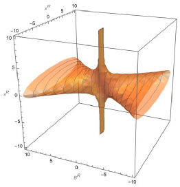
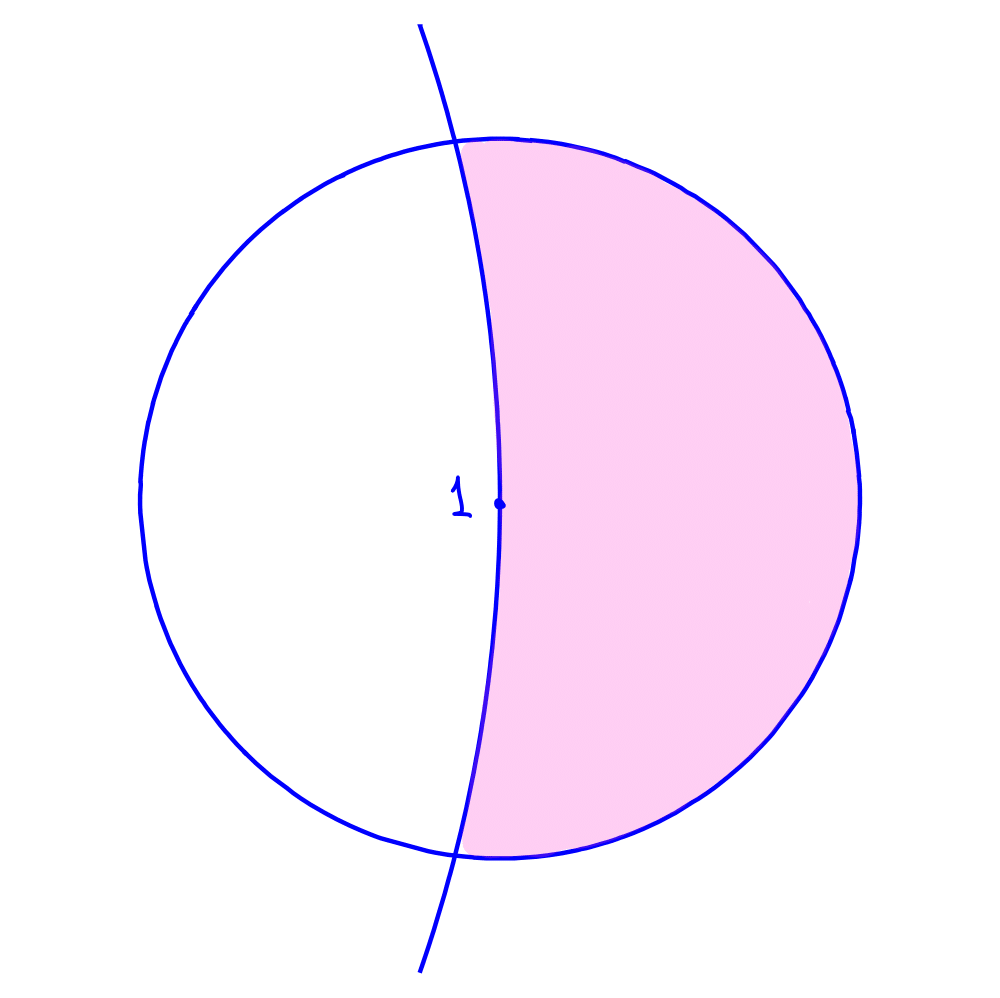
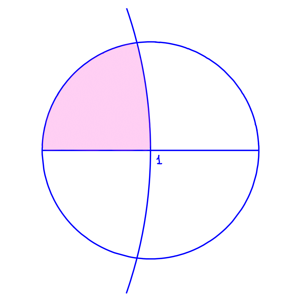
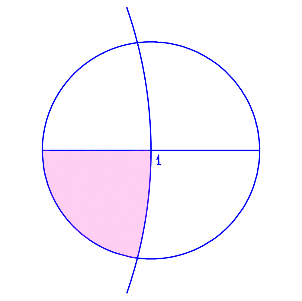
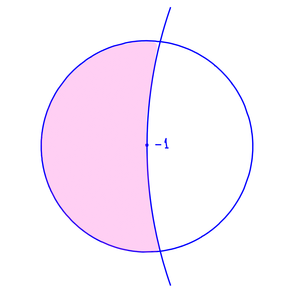
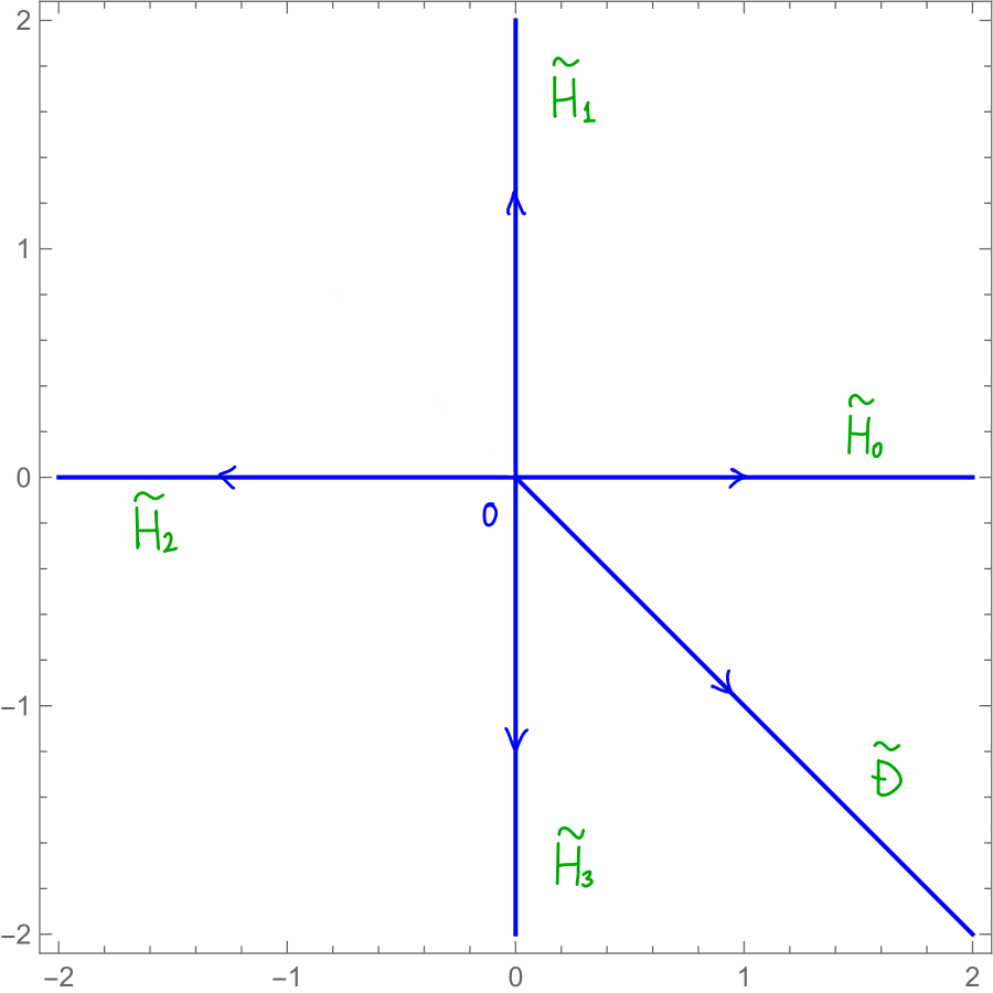
If we write and where , expression (3.1.14) implies that is parametrized by triples such that
| (3.1.15) |
see Figure 1. We shall call the set of the above triples the monodromy surface
| (3.1.16) |
We refer those who are interested in the geometry of in detail to the monograph [GH17].
What we have shown is that one can always associate the monodromy data to each solution of (1.0.3).
3.2 Riemann-Hilbert Problem for sinh-Gordon Equation
Riemann-Hilbert problems arise when one considers the inverse monodromy map
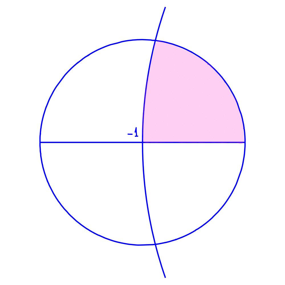
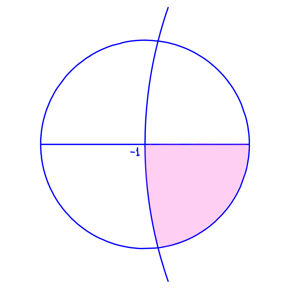
Given any , define a sectionally holomorphic in matrix function
| (3.2.1) |
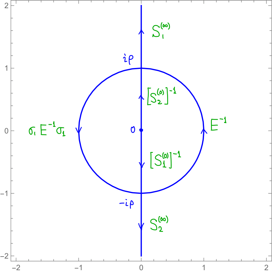
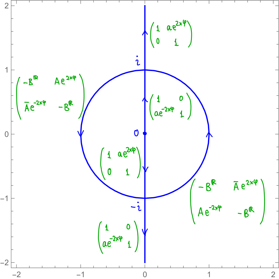
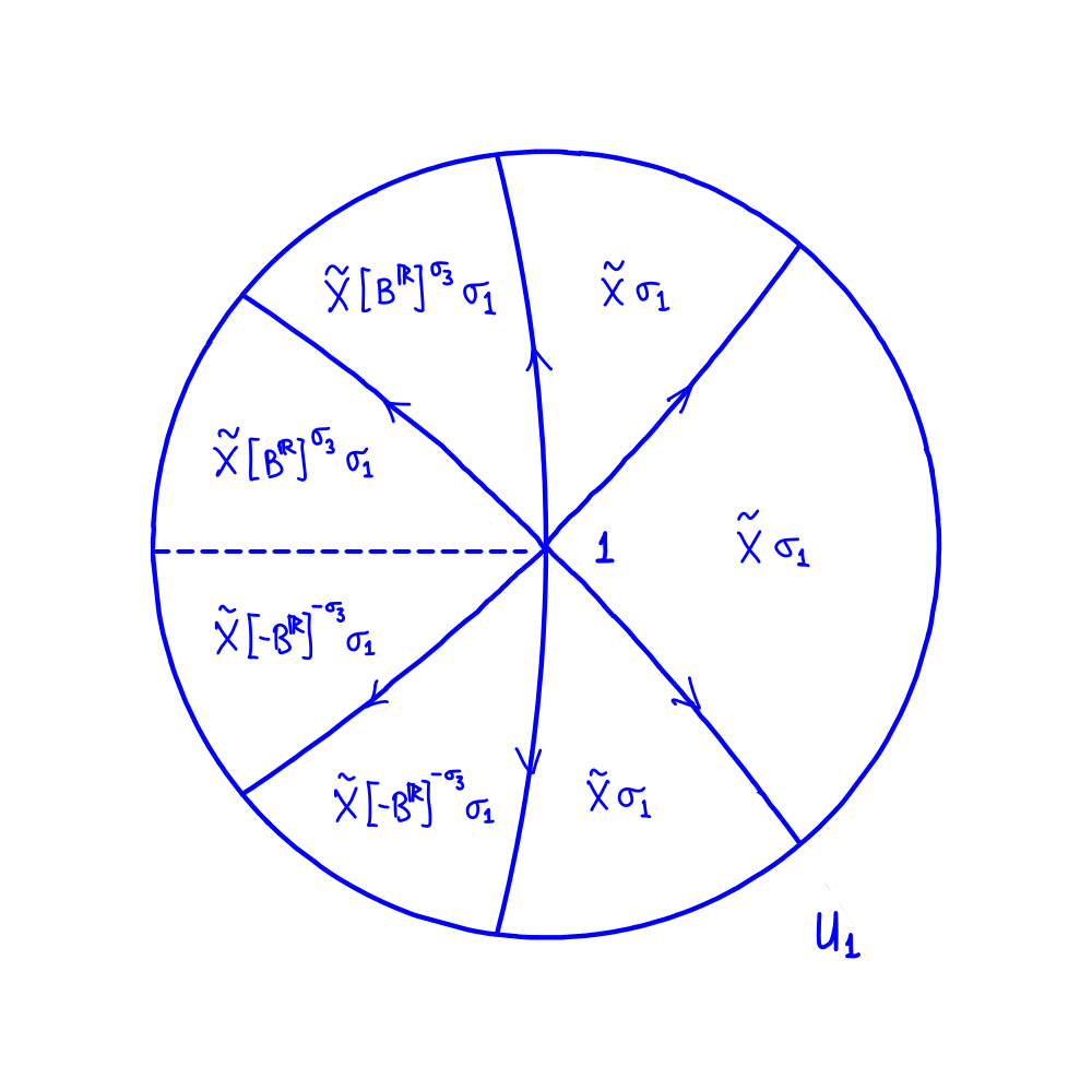
It readily follows from (3.1.8)–(3.1.11) that (3.2.1) has constant jumps on the circle and the imaginary axis as specified on Figure 2 (here, one needs to recall (3.1.7) to find the jumps on and ) as well as asymptotic behavior at given by the formal solutions . By construction, the jump matrices depend only on the monodromy data.
Conversely, let be monodromy data and and be as in (3.1.12) and (3.1.13) corresponding to . Consider the following Riemann-Hilbert problem.
Riemann-Hilbert Problem 1.
Find a matrix function such that
-
(1)
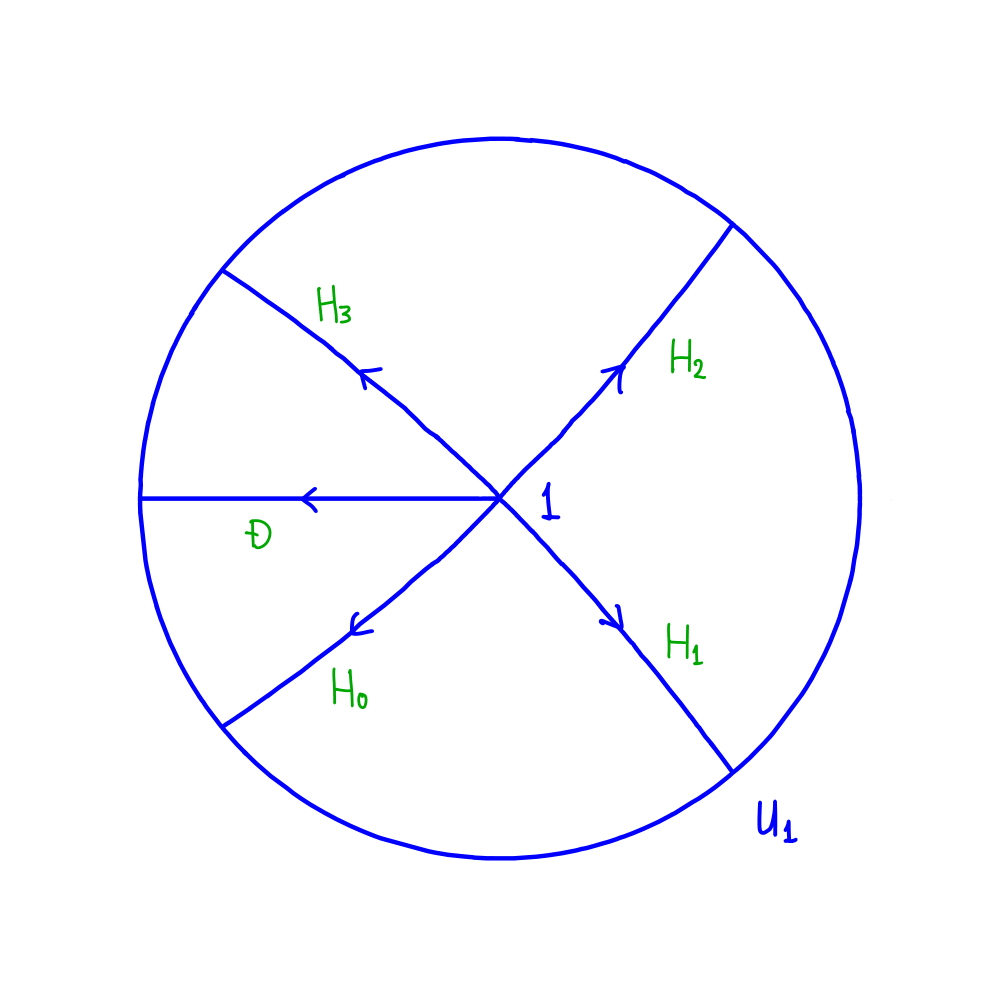
sectional analyticity: is analytic for , where the oriented contour is depicted in Figure 2;
-
(2)
jump condition: one-sides traces defined by
where a subscript (resp. ) refers to a limit to the oriented contour from its left (resp. right) side, exists a.e. on , belong to , and satisfy
where the jump matrices on are as on Figure 2;
-
(3)
normalization conditions: it holds that
(3.2.2)
It is a non-trivial but standard result in integrable systems, see for example [FIKN06, Theorem 5.4] and [IN11], that the solution of the above problem exists and is meromorphic in , determines solutions of (2.0.7) via (3.2.1), and allows one to recover the corresponding solution of (1.0.3) via asymptotics around the origin. The proof of Theorem 2.1 proceeds by asymptotically analyzing RHP 1 for large .
Remark.
The choice of , see (3.1.17), does not affect real solutions of (1.0.3). Indeed, let be the solution of (1.0.3) corresponding to some and and be the corresponding solution of RHP 1. Define
One can readily see that satisfies RHP 1(2) with jump matrices corresponding to the same and . Because and we define real solutions as solutions that are real modulo addition of integer multiples of , is in fact the solution of RHP 1 corresponding to and . Thus, , the solution of (1.0.3) corresponding to and , is equal to .
3.3 Riemann-Hilbert Problem for sine-Gordon Equation
The direct monodromy problem for the sine-Gordon equation is well known, see for example [FIKN06, Chapter 13] or [Nil09], and can be deduced in the same way as above. Following [Nil09], the monodromy data for all (not necessarily real) solutions of (1.0.4) consist of Stokes matrices
| (3.3.1) |
as well as the connection matrix
| (3.3.2) |
where the first case is known as special case and the second one as the general case. Again, exactly as in the case of the sinh-Gordon equation, the inverse monodromy problem relies on the following Riemann-Hilbert problem.
Riemann-Hilbert Problem 2.
As usual, (3.3.3) describes asymptotics of the formal fundamental solutions of the first equation in (2.0.13) at .
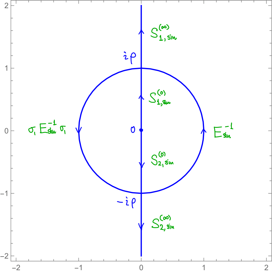
Recall that Lax pair (2.0.13) can be transformed into (2.0.7) by setting either or and making a change of variables . Notice that the first gauge transformation takes the formal fundamental solution of (2.0.13) around into the formal fundamental solutions of (2.0.7) around while the second one provides correspondence between the formal fundamental solutions at . Therefore, RHP 2 transforms into RHP 1 upon setting
| (3.3.4) |
The above transformation induces the following relation between monodromy data:
Using parametrization (3.1.17) of the monodromy data for sinh-Gordon equation, we get that corresponds to the special case with and corresponds to the general case with and where again . In both cases corresponds to the choice of sign in (3.3.2) and we interpret as . The choices of that cannot be parametrized by as above lead to the non-real solutions of sinh-Gordon equations.
4 Proof of Theorem 2.1
As indicated in the introduction, we shall use the nonlinear steepest descent method of Deift and Zhou [DZ93] to prove the desired asymptotics. In Section 4.1 we review the case that includes the McCoy-Tracy-Wu one-parameter family of smooth solutions (this proof has already been outlined in Niles’ thesis [Nil09, Apendix D]). Then, in Section 4.2, we consider the case .
4.1 Case 1:
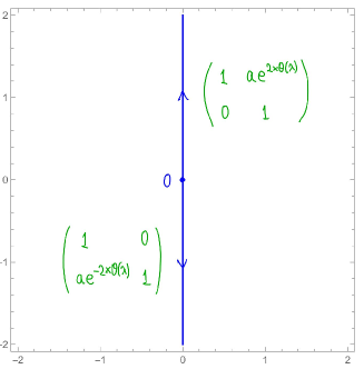
When , it readily follows from (3.1.15) that . As we pointed out in the remark of Section 3.2, it is enough to consider the case only. Then, the jump matrices on the arcs of become equal to the identity matrix. That is, has the discontinuity only along the imaginary line. Let
| (4.1.1) |
Then is the solution of the following Riemann-Hilbert problem:
Riemann-Hilbert Problem 3.
Note that when , , and when , . Thus, both jump matrices comprising exponentially decay to the identity matrix . In fact, one can show that
| (4.1.3) |
where is some constant. Hence, by the small norm theorem, see for example [FIKN06, Theorem 8.1], there exists a unique solution of RHP 3 for all large and
| (4.1.4) |
where for (hence, is the solution of the singular integral equation obtained by taking the traces of both sides of (4.1.4) on the left-hand side of ). The small norm theorem further implies that
| (4.1.5) |
for some constant . Observe that vanishes exponentially at the origin. Hence, and one has that
| (4.1.6) |
by Cauchy-Schwarz inequality, (4.1.3), and (4.1.5). Recall that
see [DLMF, Equation (10.32.9)]. Then, (4.1.6) becomes
| (4.1.7) |
On the other hand, it immediately follows from RHP 3(3) and (3.1.2) that
| (4.1.8) |
By comparing (4.1.7) with (4.1.8), we get that
as , where we used the fact that to deduce the leading order behavior of the logarithm. This finishes the proof of Theorem 2.1 in the case .
4.2 Case 2:
Now we will consider the case . Again, we only look at .
4.2.1 Opening of Lenses
Recall that in RHP 1 was arbitrary. Motivated by the scaling used in (4.1.1), we now set . Transformation (4.1.1) no longer fits our needs because in the upper half-plane while in the lower half-plane and so the jump matrices on the unit circle would always have exponentially growing entries. The next best thing one can do is to make off-diagonal entries of the jump matrices on the unit circle oscillating. To this end, consider
| (4.2.1) |
Then is the solution of the following Riemann-Hilbert problem:
Riemann-Hilbert Problem 4.
Find a matrix function such that
Let , where . Then,
| (4.2.3) |
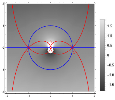
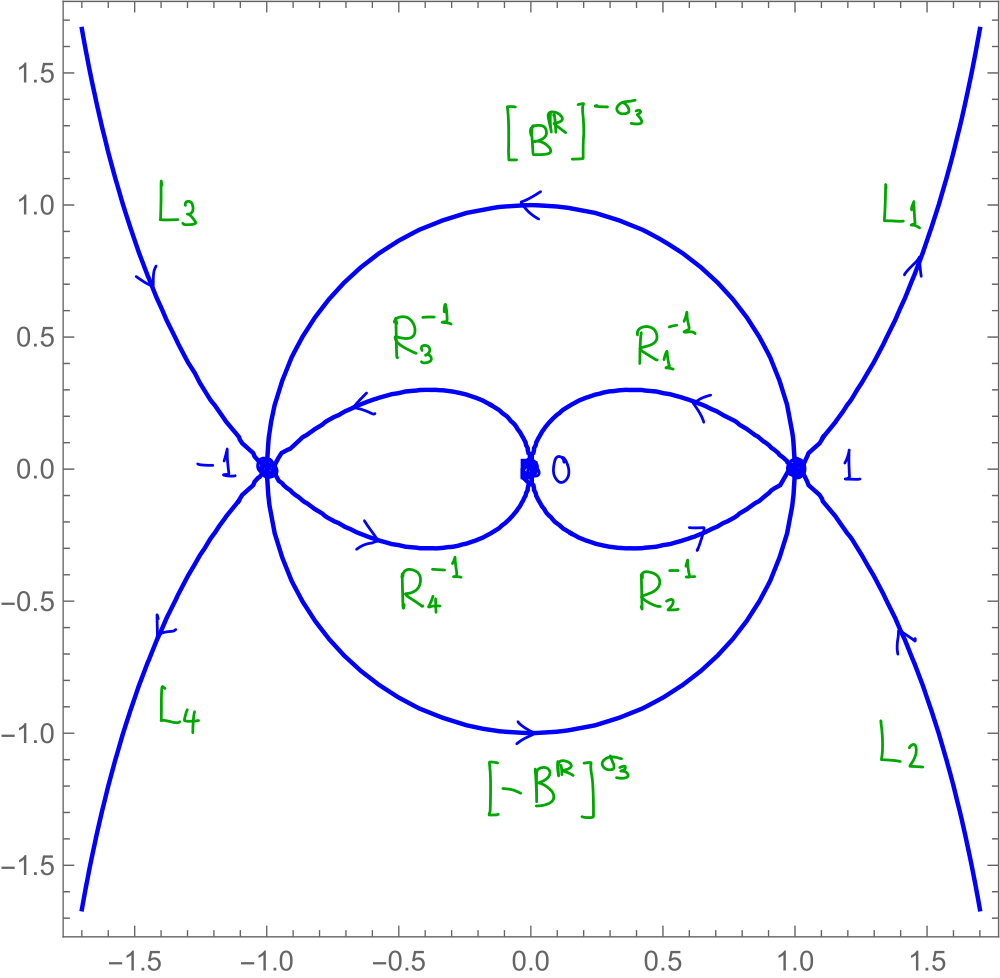
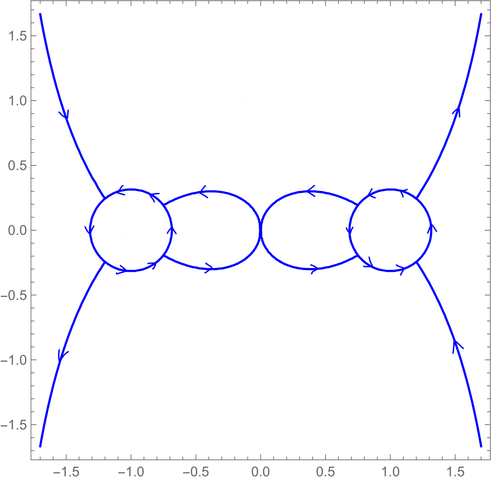
Clearly, is purely imaginary on the unit circle and therefore off-diagonal entries of on the unit circle are oscillating as desired. Notice also that the stationary points of are and . The stationary contour is shown on Figure 6.
Next, we decompose the jump matrices on the unit circle in RHP 4(2) as follows:
where
| (4.2.4) | |||
| (4.2.5) | |||
| (4.2.6) | |||
| (4.2.7) |
Using the above decomposition we define a matrix function as on Figure 7.
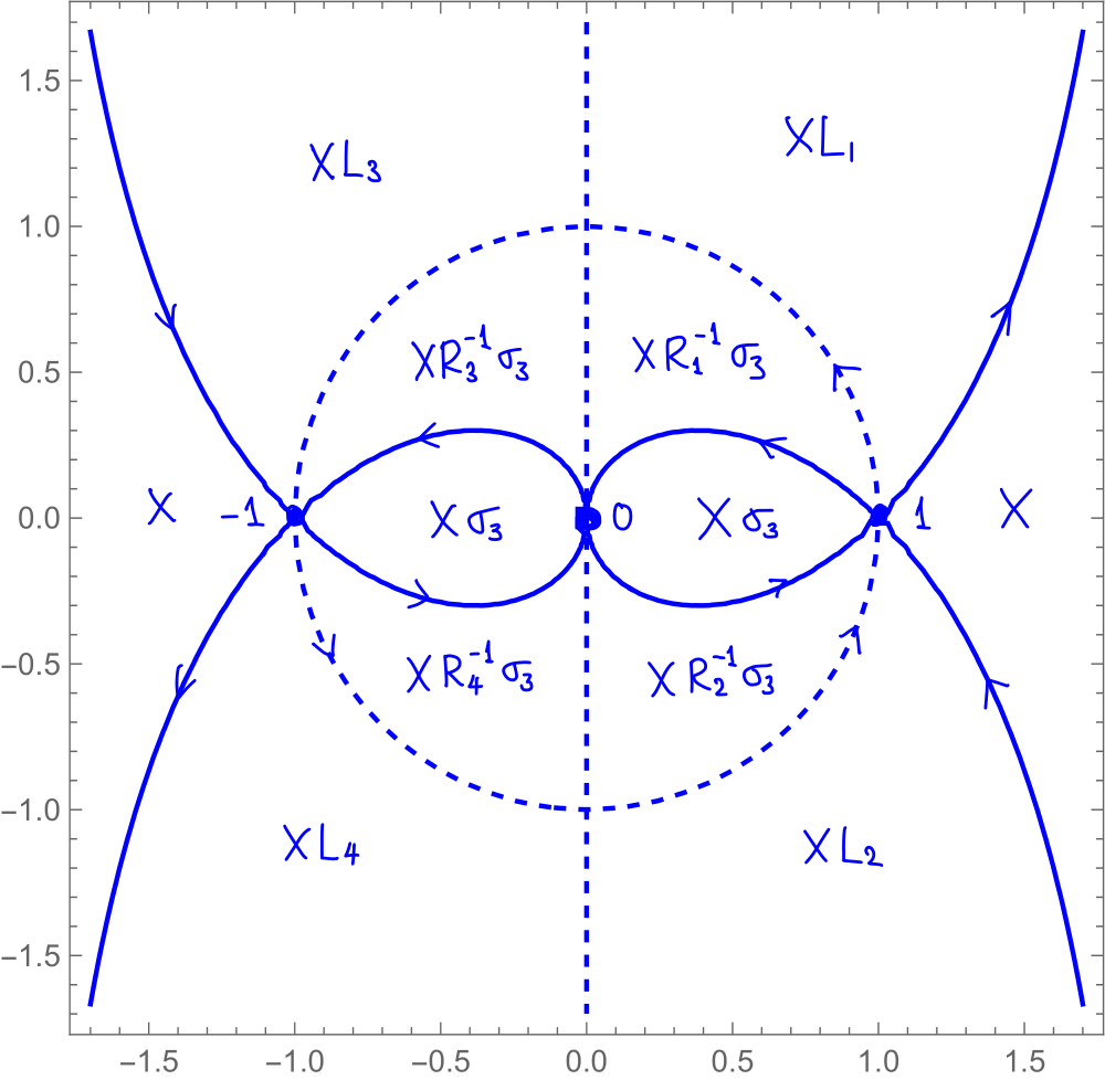
Then is the solution of the following Riemann-Hilbert problem:
Riemann-Hilbert Problem 5.
Remark.
4.2.2 The Global Parametrix
As we have mentioned above, the jump matrices in RHP 4 are close to the identity except on the unit circle (oriented counter-clockwise). As standard in the theory, we now look for a global parametrix, a solution of a Riemann-Hilbert problem with the same jump on the unit circle as in RHP 4(2). To this end, let
Consider the following model Riemann-Hilbert problem:
Riemann-Hilbert Problem 6.
Find a matrix function such that
-
(1)
is analytic for ;
-
(2)
continuous one-sides traces exists on and satisfy
where
-
(3)
it holds that as .
Lemma 4.1.
The solution of RHP 6 is given by
| (4.2.9) |
where
is holomorphic in and normalized so that , and
is holomorphic in and normalized so that .
Proof.
RHP 6(1) follows immediately from the choice of the branch cuts for , .
Notice that a linear fractional transformation maps and onto and , respectively. Then, one can readily check that
where and is the argument of that belongs to (we use here the fact that and ). Since
on the ray oriented towards the origin, it holds that
on and , respectively. This immediately shows that RHP 6(2) is fulfilled.
Finally, as , it holds that , which shows the validity of RHP 6(3) and finishes the proof of the lemma. ∎
Let be the following sub-domains of a sufficiently small neighborhood of :
Let be the branch with the cut positive for , where
| (4.2.10) |
Then, one can write the global parametrix in as
| (4.2.11) |
where is an analytic function in a neighborhood of such that .
Similarly, we define the following sub-domains of a sufficiently small neighborhood of :
Let be the branch with the cut where we take . Then, one can write the global parametrix in as
| (4.2.12) |
where is analytic in a neighborhood of and .
4.2.3 Local Parametrix at
Since the jump matrices forming are not uniformly close to the identity matrix in , we need to solve RHP 5 locally in . There are many such solutions as any of them can be multiplied by a holomorphic matrix function on the left. We seek one that matches well the global parametrix on .
To find the desired local parametrix, let us observe that the jump relations in RHP 5(2) can be changed within into the ones depicted on Figure 11B
via the transformation , see Figure 11A, where was introduced in (4.2.11) and the resulting jump matrices are given by
| (4.2.13) |
and was defined in (4.2.10). It readily follows from (4.2.1) that
| (4.2.14) |
Hence, the quadratic local form of and the structure of the jump matrices (4.2.13) lead us to the following Riemann-Hilbert problem:
Riemann-Hilbert Problem 7.
RHP 7 admits an explicit solution in terms of the parabolic cylinder functions. Namely, if we set , then is equal to
where
Recall that , , , and . Therefore,
| (4.2.16) | ||||
| (4.2.17) | ||||
| (4.2.18) |
where we used the identity for the first equality.
The fact that the above-defined matrix functions satisfy RHP 7(2) can be easily verified using the identity
Furthermore, using the asymptotic expansion formula
which holds uniformly in sectors , , one can check that
| (4.2.19) |
uniformly for , which is a refinement of RHP 7(3).
To set up correspondence between and planes, we introduce the following conformal mapping on :
| (4.2.20) |
where asymptotics at follows from (4.2.14) and also fixes the branch of the square root used in (4.2.20). Recall that the contour consists of the curves on which the real or imaginary parts of vanish. Hence, one can easily see that maps the contour on Figure 11B into .
We now define local parametrix by setting
where the matrix has the same jumps in as and is a holomorphic prefactor, see (4.2.11), given by
4.2.4 Local Parametrix at
The local parametrix is constructed similarly. First, we transform plane into plane via the conformal map
| (4.2.22) |
where the asymptotic formula holds as and the value fixes the branch of the square root used to define the map. Again, one can see that takes the stationary contour into the coordinate axes.
4.2.5 Small Norm Problem
We look for the solution of RHP 5 in the form
| (4.2.26) |
where the error function solves of the following Riemann-Hilbert problem.
Riemann-Hilbert Problem 8.
Find a matrix function such that
-
(1)
is analytic for , where , see Figure 13, is given by
-
(2)
one-sides traces exists a.e. on , belong to , and satisfy
where
(4.2.27) -
(3)
it holds that
It readily follows from (4.2.18) and Lemmas 4.2–4.3 that the jump is not uniformly close to on as . To circumvent this difficulty, let
We look for the solution of RHP 8 in the form
| (4.2.28) |
where solves the following Riemann-Hilbert problem.
Riemann-Hilbert Problem 9.
Find a matrix function such that
-
(1)
is analytic for , where is the same as in RHP 8;
-
(2)
one-sides traces exists a.e. on , belong to , and satisfy
where
(4.2.29) -
(3)
it holds that
- (4)
It readily follows from Lemmas 4.2–4.3 and (4.2.32) that
| (4.2.33) |
Moreover, it follows from (4.2.4), (4.2.5), (4.2.6), (4.2.7) that the absolute value of the only non-zero entry of on is equal to , see Figure 8. Recall also that is the set where . We then get from (4.2.3) that
| (4.2.34) |
where . This expression shows that on , where constant depends on the radii of and . Observe also that lies within the strip and is asymptotic to the vertical lines . Hence, we can conclude that
| (4.2.35) |
for a possibly adjusted constant and any . Altogether, we have that RHP 9 is a small norm problem. However, has poles. Following the dressing technique of [BI12], we look for the solution of RHP 9 in the form
| (4.2.36) |
where the matrix will be specified shortly and solves the following (small norm) Riemann-Hilbert problem.
Riemann-Hilbert Problem 10.
Find a matrix function such that
-
(1)
is analytic for , where is the same as in RHP 8;
-
(2)
one-sides traces exists a.e. on , belong to , and satisfy
where
(4.2.37) -
(3)
it holds that
This Riemann-Hilbert problem can be solved as in Section 4.1 because
| (4.2.38) |
by (4.2.33) and (4.2.35). Hence, provided we can choose matrix so that as in (4.2.36) solves RHP 9, we can solve all the previous Riemann-Hilbert problems. Matrix is algebraically determined by residue conditions (4.2.30) and (4.2.31). Write . Then,
by (4.2.36). It is a tedious but straightforward computation to verify that
As a solution of a small norm Riemann-Hilbert problem, is unique and therefore . Write . Then,
| (4.2.39) |
Write . Then, we get from (4.2.30) and (4.2.31) that
| (4.2.40) |
where and are the standard coordinate vectors in . Thus, symmetry (4.2.39) at now implies that
Since is a solution of a small norm problem, as by (4.2.38), see the next subsection. Because , see (4.2.32), we can further deduce that
provided the denominator above is non-zero. Using (4.2.32), we then get that
| (4.2.41) |
4.2.6 Asymptotic Analysis
Exactly as in Section 4.1, by the small norm theorem, the unique solution of RHP 10 is given by
| (4.2.42) | ||||
| (4.2.43) |
for , where , , which itself is a solution of the corresponding integral equation. By (4.2.38), the small norm theorem implies that
| (4.2.44) |
In particular, we get that by (4.2.38), (4.2.44), and the Cauchy-Schwarz inequality as claimed before. This means that if is the increasing sequence of values of for which the matrix cannot be constructed, i.e., the denominator in (4.2.41) vanishes, then
for all large enough. The above relations readily yield asymptotic formula (2.0.4).
Next, we can infer from (4.2.34) that is tangential to the imaginary axis at the origin and that vanishes exponentially there with respect to . Hence, as in Section 4.1, is well defined and it holds that
by (4.2.43), where the second integral is estimated by Cauchy-Schwarz inequality, (4.2.38), and (4.2.44), while -norms of can be estimated around the origin using (4.2.35) and exponential vanishing of the integrand at . Recall now that , see Lemma 4.1. Then, it follows from (4.2.8), (4.2.26), (4.2.28), and (4.2.36) that
Thus, we get from (3.1.2) and (4.2.41) that
| (4.2.45) | ||||
| (4.2.46) |
Since we defined real solutions modulo addition of integer multiples of , the above formula readily yields (2.0.1).
Appendix A Connection Problem for Real Solutions of Painlevé III
In this appendix we connect the behavior as and of the real solutions of (1.0.2) with and . Recall that if is such a solution, then so are and . Thus, we will only describe solutions that correspond to , real solutions of (1.0.3), via
| (A.0.1) |
As explained in (3.1.17), real solutions of (1.0.3) are parametrized by pairs , where and . Moreover, as pointed out in the remark at the end of Section 3.2, , . This means that
| (A.0.2) |
and therefore it is enough to consider the case as was done in the proof of Theorem 2.1. Next, one can readily see using (3.1.12) and (3.1.14) that solves RHP 1 when does, but with the monodromy data replaced by , that is, replaced by when is finite and replaced by when . One can also readily check that , see (3.1.2). Hence,
| (A.0.3) |
when is finite and infinite, respectively (the case and corresponds to the trivial solutions ). In particular, it is sufficient for us to consider only solutions with ( when ). Altogether, below we assume (A.0.1) and take , .
We get from (4.1.7) and (4.1.8) as well as (4.2.46) that
| (A.0.4) |
as . The corresponding formulae as now need to be deduced from [Nil09, Section 3]. As this reference does not include final computations, we felt compelled to provide them below. To this end, we recall that , where is the solution of (1.0.4). Then
Let be as in (3.3.3). When , it is stated on [Nil09, pages 60 and 63] that
where we will introduce the symbols , and further below, while
see [Nil09, pages 56-57] and recall that we take . Multiplying out the above product gives
which, in turn, yields that
| (A.0.5) |
Let now . In this case and , where was introduced in Theorem 2.2, see [Nil09, pages 55 and 60]. Recall further that we set in this case (when ). Hence, by noticing that and after some straightforward simplifications, we get that
where we treat the last fraction as when . Thus, using Euler’s reflection formula for the gamma function, we can conclude that
| (A.0.6) |
Let now . In this case , where was introduced in Theorem 2.2, and
see [Nil09, pages 61 and 63]. Thus, it holds that
where (and therefore ) and we treat the above fractions as when . Hence, it holds that
where was introduced in Theorem 2.2. Consequently, we get from (A.0.5) that
| (A.0.7) |
where we used the identity .
Finally, let , i.e., . Then, it holds that
see [Nil09, pages 64-67], where
(as in Theorem 2.2, is the Euler’s constant) and the explicit expression for is not important to us. Therefore, exactly as in the previous cases it holds that
| (A.0.8) |
Formulae (A.0.4), (A.0.6)–(A.0.8) together with symmetries (A.0.2) and (A.0.3) finish the description of the connection formulae for the real solutions (on ) of Painlevé III() equation (1.0.2) with .
Appendix B On Li’s Conjecture
The conjecture raised in [Li24] concerns the connection between behavior at infinity and near zero of the radial solutions of (2.0.6). In the special case it is assumed that a solution of (2.0.6) satisfies
| (B.0.1) |
as , from which the behavior at the origin is inferred. More precisely, set
see [Li24, Equations (2.2) and (4.1)] ( and in the considered special case, where we also used Legendre duplication formula). It is then claimed, see cases of [Li24, Conjecture 4.1], that
| (B.0.2) |
as with being smooth on , where .
Clearly, in the considered special case, is a solution of the tt∗-Toda equation (1.0.1) and therefore solves the sinh-Gordon Painlevé III equation (1.0.3). Assumption (B.0.1) and Theorem 2.1 immediately imply that is the solution corresponding to and . It then follows that
where are the same as in Theorem 2.2 and we used conjugate symmetry of the Gamma function. Hence,
according to (B.0.2). Since , the conjecture now follows from (A.0.1), the second formula in (A.0.3), and (A.0.7).
References
- [BI12] Thomas Bothner and Alexander Its. The nonlinear steepest descent approach to the singular asymptotics of the second Painlevé transcendent. Phys. D, 241(23-24):2204–2225, 2012.
- [BMW73] Eytan Barouch, Barry M. McCoy, and Tai Tsun Wu. Zero-field susceptibility of the two-dimensional ising model near . Phys. Rev. Lett., 31:1409–1411, Dec 1973.
- [CV91] Sergio Cecotti and Cumrun Vafa. Topological–anti-topological fusion. Nuclear Phys. B, 367(2):359–461, 1991.
- [CV92] S. Cecotti and Cumrun Vafa. Exact results for supersymmetric models. Phys. Rev. Lett., 68(7):903–906, 1992.
- [CV93] Sergio Cecotti and Cumrun Vafa. On classification of supersymmetric theories. Comm. Math. Phys., 158(3):569–644, 1993.
- [DLMF] NIST Digital Library of Mathematical Functions. https://dlmf.nist.gov/, Release 1.2.2 of 2024-09-15. F. W. J. Olver, A. B. Olde Daalhuis, D. W. Lozier, B. I. Schneider, R. F. Boisvert, C. W. Clark, B. R. Miller, B. V. Saunders, H. S. Cohl, and M. A. McClain, eds.
- [DZ93] P. Deift and X. Zhou. A steepest descent method for oscillatory Riemann-Hilbert problems. Asymptotics for the MKdV equation. Ann. of Math. (2), 137(2):295–368, 1993.
- [FIKN06] Athanassios S. Fokas, Alexander R. Its, Andrei A. Kapaev, and Victor Yu. Novokshenov. Painlevé transcendents, volume 128 of Mathematical Surveys and Monographs. American Mathematical Society, Providence, RI, 2006. The Riemann-Hilbert approach.
- [FN80] Hermann Flaschka and Alan C. Newell. Monodromy- and spectrum-preserving deformations. I. Comm. Math. Phys., 76(1):65–116, 1980.
- [GH17] Martin A. Guest and Claus Hertling. Painlevé III: a case study in the geometry of meromorphic connections, volume 2198 of Lecture Notes in Mathematics. Springer, Cham, 2017.
- [GIK+23] Martin A. Guest, Alexander R. Its, Maksim Kosmakov, Kenta Miyahara, and Ryosuke Odoi. Connection formulae for the radial Toda equations I, 2023. arXiv:2309.16550.
- [GIL15a] Martin A. Guest, Alexander R. Its, and Chang-Shou Lin. Isomonodromy aspects of the equations of Cecotti and Vafa I. Stokes data. Int. Math. Res. Not. IMRN, (22):11745–11784, 2015.
- [GIL15b] Martin A. Guest, Alexander R. Its, and Chang-Shou Lin. Isomonodromy aspects of the tt* equations of Cecotti and Vafa II: Riemann-Hilbert problem. Comm. Math. Phys., 336(1):337–380, 2015.
- [GIL20] Martin A. Guest, Alexander R. Its, and Chang-Shou Lin. Isomonodromy aspects of the tt* equations of Cecotti and Vafa III: Iwasawa factorization and asymptotics. Comm. Math. Phys., 374(2):923–973, 2020.
- [GIL23] Martin A. Guest, Alexander R. Its, and Chang-Shou Lin. The tt*-toda equations of n type, 2023. arXiv:2302.04597.
- [GL14] Martin A. Guest and Chang-Shou Lin. Nonlinear PDE aspects of the tt* equations of Cecotti and Vafa. J. Reine Angew. Math., 689:1–32, 2014.
- [IN11] Alexander Its and David Niles. On the Riemann-Hilbert-Birkhoff inverse monodromy problem associated with the third Painlevé equation. Lett. Math. Phys., 96(1-3):85–108, 2011.
- [IP16] Alexander Its and Andrei Prokhorov. Connection problem for the tau-function of the sine-Gordon reduction of Painlevé-III equation via the Riemann-Hilbert approach. Int. Math. Res. Not. IMRN, (22):6856–6883, 2016.
- [Kit87] A. V. Kitaev. The method of isomonodromic deformations and the asymptotics of the solutions of the “complete” third Painlevé equation. Mat. Sb. (N.S.), 134(176)(3):421–444, 448, 1987.
- [Li24] Yuqi Li. Smooth solutions of the tt* equation: a numerical aided case study. SIGMA Symmetry Integrability Geom. Methods Appl., 20:Paper No. 057, 2024.
- [Mik81] Alexander V. Mikhailov. The reduction problem and the inverse scattering method. Physica D: Nonlinear Phenomena, 3(1):73–117, 1981.
- [MTW77] Barry M. McCoy, Craig A. Tracy, and Tai Tsun Wu. Painlevé functions of the third kind. J. Mathematical Phys., 18(5):1058–1092, 1977.
- [Nil09] David Gregory Niles. The Riemann-Hilbert-Birkhoff inverse monodromy problem and connection formulae for the third Painleve transcendents. ProQuest LLC, Ann Arbor, MI, 2009. Thesis (Ph.D.)–Purdue University.
- [Nov84] V. Yu. Novokshënov. The method of isomonodromic deformation and the asymptotics of the third Painlevé transcendent. Funktsional. Anal. i Prilozhen., 18(3):90–91, 1984.
- [Nov85] V. Yu. Novokshënov. The asymptotic behavior of the general real solution of the third Painlevé equation. Dokl. Akad. Nauk SSSR, 283(5):1161–1165, 1985.
- [Nov86] V. Yu. Novokshënov. Movable poles of solutions of the Painlevé equation of the third type and their connection with Mathieu functions. Funktsional. Anal. i Prilozhen., 20(2):38–49, 96, 1986.
- [Nov07] V. Yu. Novokshenov. Asymptotics in the complex plane of the third Painlevé transcendent. In Difference equations, special functions and orthogonal polynomials, pages 432–451. World Sci. Publ., Hackensack, NJ, 2007.
- [Nov08] V. Yu. Novokshenov. Connection formulas for the third Painlevé transcendent in the complex plane. In Integrable systems and random matrices, volume 458 of Contemp. Math., pages 55–69. Amer. Math. Soc., Providence, RI, 2008.