Properties of the tensor state $bc\overline{b}\overline{c}$

Abstract

Spectroscopic parameters and decays of the exotic tensor meson $T$ with content $bc\overline{b}\overline{c}$ are explored in the context of the diquark-antidiquark model. We treat it as a state built of axial-vector diquark $b^{T}C\gamma_{\mu}c$ and antidiquark $\overline{b}\gamma_{\nu}C\overline{c}^{T}$, where $C$ is the charge conjugation matrix. The mass $m$ and current coupling $\Lambda$ of this tetraquark are extracted from two-point sum rules. Our result for $m=(12.70\pm 0.09)~{}\mathrm{GeV}$ proves that $T$ is unstable against strong dissociations to two-meson final states. Its dominant decay channels are processes $T\to J/\psi\Upsilon$, $\eta_{b}\eta_{c}$, and $B_{c}^{(\ast)+}B_{c}^{(\ast)-}$. Kinematically allowed transformations of $T$ include also decays $T\rightarrow D^{(\ast)+}D^{(\ast)-}$ and $D^{(\ast)0}\overline{D}^{(\ast)0}$, which are generated by $b\overline{b}$ annihilation inside of $T$ and creation later pairs of $DD$ mesons. The full width of $T$ is estimated by considering all of these channels. Their partial widths are calculated by invoking methods of three-point sum rule approach which are required to evaluate strong couplings at corresponding tetraquark-meson-meson vertices. Our predictions for the mass and width $\Gamma_{T}=(108.4\pm 15.4)~{}\mathrm{MeV}$ of the tensor state $T$ provide useful information for experimental studies of fully heavy four-quark exotic structures.

I Introduction

During last years, investigation of fully heavy four-quark mesons has become one of interesting and rapidly growing branches of high energy physics. The main reason for such interest, besides pure theoretical arguments, is observation of four $X$ structures with masses in a range $6.2-7.3\ \mathrm{GeV}$ by LHCb-ATLAS-CMS collaborations LHCb:2020bwg ; Bouhova-Thacker:2022vnt ; CMS:2023owd . According to overwhelming opinion they are scalar resonances composed of $cc\overline{c}\overline{c}$ quarks, thought there exist kinematical explanations of their origin as well.

These discoveries generated numerous and interesting publications devoted to study of newly observed structures Zhang:2020xtb ; Albuquerque:2020hio ; Yang:2020wkh ; Becchi:2020mjz ; Becchi:2020uvq ; Wang:2022xja ; Faustov:2022mvs ; Niu:2022vqp ; Dong:2022sef ; Yu:2022lak ; Kuang:2023vac ; Wang:2023kir ; Dong:2020nwy ; Liang:2021fzr . The $X$ resonances were explored also in the QCD sum rule framework in our articles Agaev:2023wua ; Agaev:2023ruu ; Agaev:2023gaq ; Agaev:2023rpj , in which we modeled them as diquark-antidiquark and hadronic molecule states. This analysis allowed us to propose our assignments for these resonances. Thus, some of them were interpreted as a pure ground-level diquark-antidiquark Agaev:2023wua and hadronic molecule Agaev:2023ruu states, or as admixtures of these two structures Agaev:2023gaq ; Agaev:2023rpj .

Exotic mesons containing only heavy quarks were objects of theoretical investigations starting from first days of the quark model and quantum chromodynamics which do not forbid existence of four-five quark, pure gluon or quark-gluon systems. Experimental achievements renewed and intensified interest to these exotic particles. A class of hidden charm-bottom tetraquarks $bc\overline{b}\overline{c}$ are evidently among such hadrons. The structures $bc\overline{b}\overline{c}$ were not discovered yet, but have real chances to be seen in ongoing and future experiments Carvalho:2015nqf ; Abreu:2023wwg .

Features of tetraquarks $bc\overline{b}\overline{c}$ with different spin-parities were considered in the literature Faustov:2022mvs ; Wu:2016vtq ; Liu:2019zuc ; Chen:2019vrj ; Bedolla:2019zwg ; Cordillo:2020sgc ; Weng:2020jao ; Yang:2021zrc ; Hoffer:2024alv . The masses of tetraquarks $bc\overline{b}\overline{c}$ are main parameters calculated in these articles using numerous methods. Information about partial widths of their decay modes is either scarce or absent. In other words, our knowledge about properties of exotic mesons $bc\overline{b}\overline{c}$ is rather limited. These circumstances, as well as discrepancies in predictions for the masses made in the different publications necessitate detailed studies of the tetraquarks $bc\overline{b}\overline{c}$.

In Refs. Agaev:2024wvp ; Agaev:2024mng , we investigated the scalar and axial-vector particles $bc\overline{b}\overline{c}$ and determined their masses and widths. In the present paper, we extend our analysis by considering the tensor tetraquark $bc\overline{b}\overline{c}$ with spin-parity $J^{\mathrm{PC}}=2^{+}$. For simplicity, we label it $T$ and calculate the mass and full width of this exotic meson. To find the mass $m$ and current coupling $\Lambda$, we use the two-point sum rule (SR) method Shifman:1978bx ; Shifman:1978by . Partial widths of numerous decay channels of $T$ are computed by invoking the three-point sum rule approach. This is necessary to estimate strong couplings at relevant tetraquark-meson-meson vertices which determine widths of processes under analysis.

There are a few types of decay modes of the tetraquark $T$. Decays to pairs of quarkonia $J/\psi\Upsilon$ and $\eta_{b}\eta_{c}$, as well as processes $T\rightarrow B_{c}^{\ast+}B_{c}^{\ast-}$ and $B_{c}^{+}B_{c}^{-}$ are dissociations of the initial particle to final-state mesons. In these decays all constituent quarks form the final-state conventional mesons and they are dominant channels of $T$. Second kind of decays are triggered by $b\overline{b}$ annihilation in the tetraquark to light quarks leading to generation of $DD$ pairs with suitable electric charges and spin-parities. In the case of the tensor tetraquark, we limit ourselves by investigation of four decays $T\rightarrow D^{(\ast)+}D^{(\ast)-}$ and $D^{(\ast)0}\overline{D}^{(\ast)0}$.

This work is composed of the following parts: In Sec. II, we calculate the mass and current coupling of the tensor state $T$. Partial widths of decays $T\rightarrow J/\psi\Upsilon$ and $\eta_{b}\eta_{c}$ are computed in Sec. III. The processes with $B_{c}^{(\ast)+}B_{c}^{(\ast)-}$ mesons in final states are considered in the next section IV. Partial widths of the decays $T\rightarrow D^{(\ast)+}D^{(\ast)-}$ and $D^{(\ast)0}\overline{D}^{(\ast)0}$ are evaluated in Sec. V. In this section, we also evaluate the full width of the tensor tetraquark $T$. We make our conclusions in the last part of the paper VI.

II Mass $m$ and current coupling $\Lambda$ of the tetraquark $T$

Spectroscopic parameters of the tetraquark $T$ are quantities which characterize this particle and determine its possible decay modes. The mass $m$ and current coupling $\Lambda$ of a particle can be evaluated using different approaches. One of the effective nonperturbative tools to find these parameters is the two-point sum rule method Shifman:1978bx ; Shifman:1978by . Originally invented to study parameters of ordinary baryons and mesons, it can be successfully applied for analysis of exotic hadrons as well.

In the framework of this method one has to extract SRs for $m$ and $\Lambda$, which can be done by considering the correlation function

$$\Pi_{\mu\nu\alpha\beta}(p)=i\int d^{4}xe^{ipx}\langle 0|\mathcal{T}\{J_{\mu\nu}(x)J_{\alpha\beta}^{{\dagger}}(0)\}|0\rangle,$$ (1)

where $J_{\mu\nu}(x)$ is the interpolating current for the tensor tetraquark and $\mathcal{T}$  is the time-ordering product of two currents.

Analytical expression of $J_{\mu\nu}(x)$ depends on a diquark-antidiquark model chosen for the particle. In the present article, we consider $T$ as a diquark-antidiquark structure composed of an axial-vector diquark $b^{T}C\gamma_{\mu}c$ and antidiquark $\overline{b}\gamma_{\nu}C\overline{c}^{T}$. Accordingly, the interpolating current $J_{\mu\nu}(x)$ has the following form

$$J_{\mu\nu}(x) = b_{a}^{T}(x)C\gamma_{\mu}c_{b}(x)\left[\overline{b}_{a}(x)\gamma_{\nu}C\overline{c}_{b}^{T}(x)\right.$$ (2)

$$\left.-\overline{b}_{b}(x)\gamma_{\nu}C\overline{c}_{a}^{T}(x)\right].$$

Here, $C$ is the charge conjugation matrix, whereas $a$ and $b$ are the color indices. The current $J_{\mu\nu}$ describes the tetraquark with spin-parities $J^{\mathrm{P}}=2^{+}$.

To find the sum rules for the mass $m$ and current coupling $\Lambda$, we first have to compute the correlation function $\Pi_{\mu\nu\alpha\beta}(p)$ using physical parameters of the tetraquark. For these purposes, we insert into Eq. (1) a full set of states with the quark content and spin-parities of the tetraquark $T$, and integrate it over the variable $x$. Then the correlator becomes equal to

$$\Pi_{\mu\nu\alpha\beta}^{\mathrm{Phys}}(p)=\frac{\langle 0|J_{\mu\nu}|T(p,\epsilon)\rangle\langle T(p,\epsilon)|J_{\alpha\beta}^{{\dagger}}|0\rangle}{m^{2}-p^{2}}+\cdots,$$ (3)

where the term in Eq. (3) is the contribution of the ground-state particle $T$, whereas the dots show contributions of higher resonances and continuum states. Here, $\epsilon=\epsilon_{\mu\nu}^{(\lambda)}(p)$ is the polarization tensor of the tetraquark $T$. For further calculations, it is convenient to introduce the matrix element

$$\langle 0|J_{\mu\nu}|T(p,\epsilon(p)\rangle=\Lambda\epsilon_{\mu\nu}^{(\lambda)}(p).$$ (4)

Combining Eqs. (3) and (4) and performing summation over polarization tensor using

$$\sum\limits_{\lambda}\epsilon_{\mu\nu}^{(\lambda)}(p)\epsilon_{\alpha\beta}^{\ast(\lambda)}(p) = \frac{1}{2}(\widetilde{g}_{\mu\alpha}\widetilde{g}_{\nu\beta}+\widetilde{g}_{\mu\beta}\widetilde{g}_{\nu\alpha})$$ (5)

$$-\frac{1}{3}\widetilde{g}_{\mu\nu}\widetilde{g}_{\alpha\beta},$$

where

$$\widetilde{g}_{\mu\nu}=-g_{\mu\nu}+\frac{p_{\mu}p_{\nu}}{p^{2}},$$ (6)

we find $\Pi_{\mu\nu\alpha\beta}^{\mathrm{Phys}}(p)$. Our computations yield

$$\Pi_{\mu\nu\alpha\beta}^{\mathrm{Phys}}(p) = \frac{\Lambda^{2}}{m^{2}-p^{2}}\left\{\frac{1}{2}\left(g_{\mu\alpha}g_{\nu\beta}+g_{\mu\beta}g_{\nu\alpha}\right)\right.$$ (7)

$$\left.+\text{other structures}\right\}+..,$$

with ellipses standing for contributions of other structures as well as higher resonances and continuum states. Note that, after application of Eqs. (5) and (6) there appear numerous Lorentz structures in the curly brackets. The term proportional to $(g_{\mu\alpha}g_{\nu\beta}+g_{\mu\beta}g_{\nu\alpha})$ contains contribution of only spin-$2$ particle, whereas remaining components in Eq. (7) are formed due to contributions of spin-$0$ and -$1$ states as well. Therefore, in our studies we restrict ourselves by exploring this term and corresponding invariant amplitude $\Pi^{\mathrm{Phys}}(p^{2})$.

At next phase of investigations, we compute the correlator $\Pi_{\mu\nu\alpha\beta}(p)$ with some accuracy in the operator product expansion ($\mathrm{OPE}$) using quark-gluon degrees of freedom. To this end, we have to insert the explicit expression of the current $J_{\mu\nu}(x)$ into Eq. (1) and contract relevant quark fields to obtain $\Pi_{\mu\nu\alpha\beta}^{\mathrm{OPE}}(p)$. As a result, we find

$$\Pi_{\mu\nu\alpha\beta}^{\mathrm{OPE}}(p)=i\int d^{4}xe^{ipx}\mathrm{Tr}\left[\gamma_{\alpha}\widetilde{S}_{b}^{aa^{\prime}}(x)\gamma_{\mu}S_{c}^{bb^{\prime}}(x)\right]$$

$$\times\left\{\mathrm{Tr}\left[\gamma_{\nu}\widetilde{S}_{c}^{b^{\prime}b}(-x)\gamma_{\beta}S_{b}^{a^{\prime}a}(-x)\right]-\mathrm{Tr}\left[\gamma_{\nu}\widetilde{S}_{c}^{a^{\prime}b}(-x)\right.\right.,$$

$$\left.\times\gamma_{\beta}S_{b}^{b^{\prime}a}(-x)\right]+\mathrm{Tr}\left[\gamma_{\nu}\widetilde{S}_{c}^{a^{\prime}a}(-x)\gamma_{\beta}S_{b}^{b^{\prime}b}(-x)\right]$$

$$\left.-\mathrm{Tr}\left[\gamma_{\nu}\widetilde{S}_{c}^{b^{\prime}a}(-x)\gamma_{\beta}S_{b}^{a^{\prime}b}(-x)\right]\right\},$$ (8)

where

$$\widetilde{S}_{b(c)}(x)=CS_{b(c)}^{T}(x)C,$$ (9)

and $S_{b(c)}(x)$ are $b$ and $c$ quarks’ propagators

$$S_{Q}^{ab}(x)=i\int\frac{d^{4}k}{(2\pi)^{4}}e^{-ikx}\Bigg{\{}\frac{\delta_{ab}\left({\not{k}}+m_{Q}\right)}{k^{2}-m_{Q}^{2}}$$

$$-\frac{g_{s}G_{ab}^{\alpha\beta}}{4}\frac{\sigma_{\alpha\beta}\left({\not{k}}+m_{Q}\right)+\left({\not{k}}+m_{Q}\right)\sigma_{\alpha\beta}}{(k^{2}-m_{Q}^{2})^{2}}$$

$$+\frac{g_{s}^{2}G^{2}}{12}\delta_{ab}m_{Q}\frac{k^{2}+m_{Q}{\not{k}}}{(k^{2}-m_{Q}^{2})^{4}}+\cdots\Bigg{\}}.$$ (10)

Here, we have introduced the notations

$$G_{ab}^{\alpha\beta}\equiv G_{A}^{\alpha\beta}\lambda_{ab}^{A}/2,\ \ G^{2}=G_{\alpha\beta}^{A}G_{A}^{\alpha\beta},\ A=1-8,$$ (11)

with $G_{A}^{\alpha\beta}$ being the gluon field-strength tensor, and $\lambda^{A}$–Gell-Mann matrices.

The heavy quark propagators depend only on gluon fields. Therefore, $\Pi_{\mu\nu\alpha\beta}^{\mathrm{OPE}}(p)$ contains only gluon vacuum condensates. In our calculations we take into account nonperturbative contributions $\sim\langle\alpha_{s}G^{2}/\pi\rangle$ and neglect terms $\sim\langle g_{s}^{3}G^{3}\rangle$.

Having extracted the structure $(g_{\mu\alpha}g_{\nu\beta}+g_{\mu\beta}g_{\nu\alpha})$ from $\Pi_{\mu\nu\alpha\beta}^{\mathrm{OPE}}(p)$ and labeled corresponding invariant amplitude as $\Pi^{\mathrm{OPE}}(p^{2})$, one can derive SRs for the mass and current coupling of the tetraquark $T$. For this purpose, we equate the amplitudes $\Pi^{\mathrm{Phys}}(p^{2})$ and $\Pi^{\mathrm{OPE}}(p^{2})$, carry out the Borel transformation and subtract effects due to higher resonances and continuum states by applying an assumption on quark-hadron duality. By this way, we determine the first SR equality. The second expression necessary to obtain SRs is calculated by applying the operator $d/d(-1/M^{2})$ to both sides of the first equality. Then, after simple manipulations, we get

$$m^{2}=\frac{\Pi^{\prime}(M^{2},s_{0})}{\Pi(M^{2},s_{0})},$$ (12)

and

$$\Lambda^{2}=e^{m^{2}/M^{2}}\Pi(M^{2},s_{0}),$$ (13)

which are the sum rules for $m$ and $\Lambda$. Here, $\Pi(M^{2},s_{0})$ is the amplitude $\Pi^{\mathrm{OPE}}(p^{2})$ after the Borel transformation and continuum subtraction. It depends on the Borel and continuum subtraction parameters $M^{2}$ and $s_{0}$. In Eq. (12), we also use the short-hand notation $\Pi^{\prime}(M^{2},s_{0})=d\Pi(M^{2},s_{0})/d(-1/M^{2})$.

The function $\Pi(M^{2},s_{0})$ can be expressed in terms of the two-point spectral density $\rho^{\mathrm{OPE}}(s)$ and a function $\Pi(M^{2})$

$$\Pi(M^{2},s_{0}) = \int_{4(m_{b}+m_{c})^{2}}^{s_{0}}ds\rho^{\mathrm{OPE}}(s)e^{-s/M^{2}}+\Pi(M^{2}).$$

The spectral density $\rho^{\mathrm{OPE}}(s)$ is extracted as imaginary part of the amplitude $\Pi^{\mathrm{OPE}}(p^{2})$ and consists of perturbative $\rho^{\mathrm{pert.}}(s)$ and nonperturbative $\rho^{\mathrm{Dim4}}(s)$ components. The nonperturbative function $\Pi(M^{2})$ is computed directly from the correlator and contains contributions that do not embraced by the spectral density. Explicit expressions for $\rho^{\mathrm{pert.}}(s)$ and $\rho^{\mathrm{Dim4}}(s)$ are lengthy and not presented here.

We need to specify the input parameters in Eqs. (12) and (13) to perform numerical computations. Some of them are universal quantities and do not depend on a problem under consideration. The masses of $b$ and $c$ quarks and gluon vacuum condensate $\langle\alpha_{s}G^{2}/\pi\rangle$ are such parameters. In present work, we use following values

$$m_{b}=4.18_{-0.02}^{+0.03}~{}\mathrm{GeV},\ m_{c}=(1.27\pm 0.02)~{}\mathrm{GeV},$$

$$\langle\alpha_{s}G^{2}/\pi\rangle=(0.012\pm 0.004)~{}\mathrm{GeV}^{4}.$$ (15)

The $m_{b}$ and $m_{c}$ are the running quark masses in the $\overline{\mathrm{MS}}$ scheme PDG:2022 . The gluon vacuum condensate was extracted from analysis of various hadronic processes in Refs. Shifman:1978bx ; Shifman:1978by .

Contrary, Borel and continuum subtraction parameters $M^{2}$ and $s_{0}$ are specific for each problem and should satisfy some standard constraints of SR computations. Dominance of the pole contribution ($\mathrm{PC}$) in extracted quantities and their stability upon variations of $M^{2}$ and $s_{0}$ as well as convergence of the operator product expansion are important conditions for correct SR analysis. To fulfill these requirements, we impose on the parameters $M^{2}$ and $s_{0}$ the following restrictions. First, the pole contribution

$$\mathrm{PC}=\frac{\Pi(M^{2},s_{0})}{\Pi(M^{2},\infty)},$$ (16)

should obey $\mathrm{PC}\geq 0.5$. The convergence of $\mathrm{OPE}$ is second important condition in the SR analysis. Because, the correlation function contains only nonperturbative dimension-$4$ term $\Pi^{\mathrm{Dim4}}(M^{2},s_{0})$, it is enough fulfilment of $\Pi^{\mathrm{Dim4}}(M^{2},s_{0})=\pm 0.05\Pi(M^{2},s_{0})$. It is worth noting that the maximum of the Borel parameter is determined from Eq. (16), whereas convergence of $\mathrm{OPE}$ allows us to fix its minimal value.

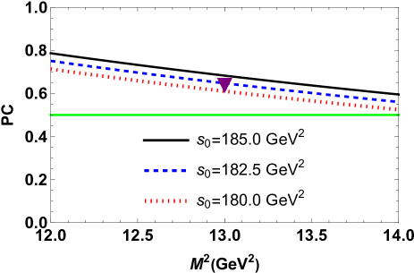
Figure 1: Dependence of $\mathrm{PC}$ on the Borel parameter $M^{2}$ at fixed $s_{0}$. The red triangle shows the point $M^{2}=13~{}\mathrm{GeV}^{2}$ and $s_{0}=182.5~{}\mathrm{GeV}^{2}$.

Our studies demonstrate that the windows

$$M^{2}\in[12,14]~{}\mathrm{GeV}^{2},\ s_{0}\in[180,185]~{}\mathrm{GeV}^{2},$$ (17)

for parameters $M^{2}$ and $s_{0}$ comply with aforementioned constraints. In fact, on the average in $s_{0}$ at maximal and minimal $M^{2}$ the pole contribution is $\mathrm{PC}\approx 0.56$, and $\approx 0.75$, respectively. The nonperturbative term is positive and at $M^{2}=12~{}\mathrm{GeV}^{2}$ forms less than $1\%$ of the whole result. The dependence of $\mathrm{PC}$ on the Borel parameter is plotted in Fig. 1, in which all curves exceed the limit line $\mathrm{PC}=0.5$.

To extract $m$ and $\Lambda$, we compute their mean values over the regions Eq. (17) and find

$$m = (12.70\pm 0.09)~{}\mathrm{GeV},$$

$$\Lambda = (2.16\pm 0.24)~{}\mathrm{GeV}^{5}.$$ (18)

Effectively, results in Eq. (18) are equal to SR predictions at the point $M^{2}=13~{}\mathrm{GeV}^{2}$ and $s_{0}=182.5~{}\mathrm{GeV}^{2}$, where $\mathrm{PC}\approx 0.65$, which guarantees the dominance of $\mathrm{PC}$ in the extracted parameters. In Fig. 2, we show $m$ as a function of $M^{2}$ and $s_{0}$.

The mass of the tensor tetraquark $T$ was evaluated in the framework of different models and methods Faustov:2022mvs ; Wu:2016vtq ; Liu:2019zuc ; Chen:2019vrj ; Bedolla:2019zwg ; Cordillo:2020sgc ; Weng:2020jao ; Yang:2021zrc . In the relativistic quark model the authors obtained $12.849\ \mathrm{GeV}$ Faustov:2022mvs . Considerably larger result, i.e., $13.59-13.599~{}\mathrm{GeV}$ was found in the color-magnetic interaction model Wu:2016vtq . The mass spectra of all-heavy tetraquarks with different contents were investigated in Ref. Liu:2019zuc , in which for the tensor state $bc\overline{b}\overline{c}$  the authors found $12.993-13.021~{}\mathrm{GeV}$. The nonrelativistic chiral quark model led to $12.809~{}\mathrm{GeV}$ Chen:2019vrj . In the relativized diquark Hamiltonian model the mass of the tensor tetraquark $2^{++}$ depending on diquarks’ spins and total spin and orbital angular momentum of the tetraquark changes from $12.576~{}\mathrm{GeV}$ till $13.65~{}\mathrm{GeV}$ Bedolla:2019zwg . Prediction $12.582~{}\mathrm{GeV}$ was made in Ref. Cordillo:2020sgc . In the extended chromomagnetic model Weng:2020jao this tensor has the mass in the range $12.537$ and $12.754~{}\mathrm{GeV}$. This problem was addressed also in the SR framework Yang:2021zrc . Values for the mass of the tensor tetraquarks $bc\overline{b}\overline{c}$ modeled by a color antitriplet-triplet and sextet-antisextet interpolating currents are equal to $12.30$ and $12.35~{}\mathrm{GeV}$, respectively.

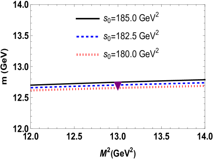
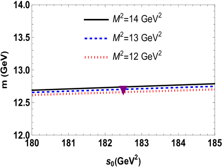
Figure 2: The mass $m$ as a function of the Borel $M^{2}$ (left panel), and continuum threshold $s_{0}$ parameters (right panel).

III Decays $T\rightarrow J/\psi\Upsilon$ and $T\rightarrow\eta_{b}\eta_{c}$

Information on the mass of the tensor state $T$ permits us to make conclusions about its decay channels. Decays to quarkonium pairs $J/\psi\Upsilon$ and $\eta_{b}\eta_{c}$ are among kinematically possible decay modes of $T$. Indeed, thresholds for creation of these final states are $12.558~{}\mathrm{GeV}$ and $12.383~{}\mathrm{GeV}$, respectively. In this section we study these decay channels of $T$ .

III.1 Process $T\rightarrow J/\psi\Upsilon$

Here, we consider the decay $T\rightarrow J/\psi\Upsilon$, the partial width of which, apart from usual input parameters, is determined by the strong coupling $g_{1}$ at the vertex $TJ/\psi\Upsilon$. The coupling $g_{1}$ can be evaluated as the form factor $g_{1}(q^{2})$ at the mass shell $q^{2}=m_{J/\psi}^{2}$.

We are going to extract the form factor $g_{1}(q^{2})$ from the three-point sum rule. To this end, we begin from analysis of the correlation function

$$\Pi_{\mu\nu\alpha\beta}(p,p^{\prime}) = i^{2}\int d^{4}xd^{4}ye^{ip^{\prime}y}e^{-ipx}\langle 0|\mathcal{T}\{J_{\mu}^{\Upsilon}(y)$$ (19)

$$\times J_{\nu}^{J/\psi}(0)J_{\alpha\beta}^{\dagger}(x)\}|0\rangle,$$

where $J_{\mu}^{\Upsilon}(x)$ and $J_{\nu}^{J/\psi}(x)$ are interpolating currents of the vector quarkonia $\Upsilon$ and $J/\psi$, respectively. They are defined as

$$J_{\mu}^{\Upsilon}(x)=\overline{b}_{i}(x)\gamma_{\mu}b_{i}(x),\ J_{\nu}^{J/\psi}(x)=\overline{c}_{j}(x)\gamma_{\nu}c_{j}(x),$$ (20)

with $i$ and $j$ being the color indices.

We need to rewrite $\Pi_{\alpha\beta\mu\nu}(p,p^{\prime})$ using the involved particles’ physical parameters. By taking into account only contributions of the ground-level particles, we recast this correlator into the form

$$\Pi_{\alpha\beta\mu\nu}^{\mathrm{Phys}}(p,p^{\prime})=\frac{\langle 0|J_{\mu}^{\Upsilon}|\Upsilon(p^{\prime},\varepsilon_{1})\rangle}{p^{\prime 2}-m_{\Upsilon}^{2}}\frac{\langle 0|J_{\nu}^{J/\psi}|J/\psi(q,\varepsilon_{2})\rangle}{q^{2}-m_{J/\psi}^{2}}$$

$$\times\langle\Upsilon(p^{\prime},\varepsilon_{1})J/\psi(q,\varepsilon_{2})|T(p,\epsilon)\rangle\frac{\langle T(p,\varepsilon)|J_{\alpha\beta}^{\dagger}|0\rangle}{p^{2}-m^{2}}+\cdots,$$

(21)

where $m_{\Upsilon}=(9460.40\pm 0.09\pm 0.04)~{}\mathrm{MeV}$ and $m_{J/\psi}=(3096.900\pm 0.006)~{}\mathrm{MeV}$ are masses of the $\Upsilon$ and $J/\psi$ mesons PDG:2022 . In the expression above, we denote by $\varepsilon_{1}$ and $\varepsilon_{2}$ the polarization vectors of these quarkonia, respectively.

To further simplify Eq. (21), it is convenient to employ the matrix elements of the mesons $\Upsilon$ and $J/\psi$

$$\langle 0|J_{\mu}^{\Upsilon}|\Upsilon(p^{\prime},\varepsilon_{1})\rangle = f_{\Upsilon}m_{\Upsilon}\varepsilon_{1\mu}(p^{\prime}),$$

$$\langle 0|J_{\nu}^{J/\psi}|J/\psi(q,\varepsilon_{2})\rangle = f_{J/\psi}m_{J/\psi}\varepsilon_{2\nu}(q).$$ (22)

Here, $f_{\Upsilon}=(708\pm 8)~{}\mathrm{MeV}$ and $f_{J/\psi}=(411\pm 7)~{}\mathrm{MeV}$ are decay constants of the mesons: Their experimental values are borrowed from Ref. Lakhina:2006vg . Besides, one should specify the matrix element of the vertex $\langle\Upsilon(p^{\prime},\varepsilon_{1})J/\psi(q,\varepsilon_{2})|T(p,\epsilon)\rangle$. A tensor-vector-vector vertex, in general, contains three independent form factors which correspond to a pair of vector mesons with helicities $\lambda=0$, $\pm 1$ and $\pm 2$ Braun:2000cs ; Aliev:2018kry ; Agaev:2024pil . In our case, we consider $g_{1}(q^{2})$ which describes to a pure $\lambda=2$ final state. Therefore, we model the vertex by the following expression

$$\langle\Upsilon(p^{\prime},\varepsilon_{1})J/\psi(q,\varepsilon_{2})|T(p,\epsilon)\rangle=g_{1}(q^{2})\epsilon_{\tau\rho}^{(\lambda)}\left[(\varepsilon_{1}^{\ast}\cdot q)\varepsilon_{2}^{\tau\ast}p^{\prime\rho}\right.$$

$$\left.+(\varepsilon_{2}^{\ast}\cdot p^{\prime})\varepsilon_{1}^{\ast\tau}q^{\rho}-(p^{\prime}\cdot q)\varepsilon_{1}^{\tau\ast}\varepsilon_{2}^{\rho\ast}-(\varepsilon_{1}^{\ast}\cdot\varepsilon_{2}^{\ast})p^{\prime\tau}q^{\rho}\right].$$

(23)

As a result, for $\Pi_{\mu\nu\alpha\beta}^{\mathrm{Phys}}(p,p^{\prime})$ we get the expression

$$\Pi_{\mu\nu\alpha\beta}^{\mathrm{Phys}}(p,p^{\prime})=g_{1}(q^{2})\frac{\Lambda f_{\Upsilon}m_{\Upsilon}f_{J/\psi}m_{J/\psi}}{\left(p^{2}-m^{2}\right)(p^{\prime 2}-m_{\Upsilon}^{2})(q^{2}-m_{J/\psi}^{2})}$$

$$\times\left[p_{\beta}^{\prime}p_{\alpha}^{\prime}g_{\mu\nu}+\frac{1}{2}p_{\mu}p_{\alpha}^{\prime}g_{\beta\nu}+\text{other structures}\right]+\cdots.$$

For the QCD side of the sum rule, we obtain

$$\Pi_{\mu\nu\alpha\beta}^{\mathrm{OPE}}(p,p^{\prime})=\int d^{4}xd^{4}ye^{ip^{\prime}y}e^{-ipx}\left\{\mathrm{Tr}\left[\gamma_{\mu}S_{b}^{ia}(y-x)\right.\right.$$

$$\left.\times\gamma_{\alpha}\widetilde{S}_{c}^{jb}(-x)\gamma_{\nu}\widetilde{S}_{c}^{bj}(x)\gamma_{\beta}S_{b}^{ai}(x-y)\right]$$

$$\left.-\mathrm{Tr}\left[\gamma_{\mu}S_{b}^{ia}(y-x)\gamma_{\alpha}\widetilde{S}_{c}^{jb}(-x)\gamma_{\nu}\widetilde{S}_{c}^{aj}(x)\gamma_{\beta}S_{b}^{bi}(x-y)\right]\right\}.$$

(25)

We utilize the structures proportional to $p_{\mu}p_{\alpha}^{\prime}g_{\beta\nu}$ and corresponding amplitudes $\Pi_{1}^{\mathrm{Phys}}(p^{2},p^{\prime 2},q^{2})$ and $\Pi_{2}^{\mathrm{OPE}}(p^{2},p^{\prime 2},q^{2})$ in both versions of the correlation function $\Pi_{\mu\nu\alpha\beta}(p,p^{\prime})$ to find SR for the form factor $g_{1}(q^{2})$. After standard operations the sum rule for $g_{1}(q^{2})$ reads

$$g_{1}(q^{2})=\frac{2(q^{2}-m_{J/\psi}^{2})}{\Lambda f_{\Upsilon}m_{\Upsilon}f_{J/\psi}m_{J/\psi}}e^{m^{2}/M_{1}^{2}}e^{m_{\Upsilon}^{2}/M_{2}^{2}}\Pi_{1}(\mathbf{M}^{2},\mathbf{s}_{0},q^{2}).$$ (26)

In Eq. (26), $\Pi_{1}(\mathbf{M}^{2},\mathbf{s}_{0},q^{2})$ is the Borel transformed and subtracted function $\Pi_{1}^{\mathrm{OPE}}(p^{2},p^{\prime 2},q^{2})$. It depends on the parameters $\mathbf{M}^{2}=(M_{1}^{2},M_{2}^{2})$ and $\mathbf{s}_{0}=(s_{0},s_{0}^{\prime})$ where the pairs $(M_{1}^{2},s_{0})$ and $(M_{2}^{2},s_{0}^{\prime})$ correspond to the tetraquark and $\Upsilon$ channels, respectively.

Requirements which should be satisfied by the auxiliary parameters $\mathbf{M}^{2}$ and $\mathbf{s}_{0}$ are universal for all SR computations and have been explained in the previous section. The form factor $g_{1}(q^{2})$ depends on the mass and current coupling of the tetraquark $T$ which have been extracted in the section II using the SR method. Therefore, beyond the regions Eq. (17) these quantities may generate large uncertainties. To exclude this problem, we use in computations for $M_{1}^{2}$ and $s_{0}$ windows Eq. (17). The parameters $(M_{2}^{2},\ s_{0}^{\prime})$ for the $\Upsilon$ channel are changed in domains

$$M_{2}^{2}\in[10,12]~{}\mathrm{GeV}^{2},\ s_{0}^{\prime}\in[98,100]~{}\mathrm{GeV}^{2}.$$ (27)

The SR method lead to reliable predictions for the form factor $g_{1}(q^{2})$ in the Euclidean region $q^{2}<0$. But the strong coupling $g_{1}$ is determined by $g_{1}(q^{2})$ at the mass shell $q^{2}=m_{J/\psi}^{2}$. Therefore, it is convenient to introduce the function $g_{1}(Q^{2})$ with $Q^{2}=-q^{2}$ and use it in analysis.The results obtained for $g_{1}(Q^{2})$ are plotted in Fig. 3, where $Q^{2}$ varies inside of limits $Q^{2}=2-30~{}\mathrm{GeV}^{2}$.

As it has been emphasized above, the strong coupling $g_{1}$ should be extracted at $q^{2}=m_{J/\psi}^{2}$, i.e., at $Q^{2}=-m_{J/\psi}^{2}$ where the SR method does not work. Therefore, we introduce the fit function $\mathcal{G}_{1}(Q^{2})$ that at momenta $Q^{2}>0$ gives the same SR data, but can be extrapolated to $Q^{2}<0$ domain. For these purposes, we utilize the function

$$\mathcal{G}_{i}(Q^{2})=\mathcal{G}_{i}^{0}\mathrm{\exp}\left[c_{i}^{1}\frac{Q^{2}}{m^{2}}+c_{i}^{2}\left(\frac{Q^{2}}{m^{2}}\right)^{2}\right],$$ (28)

where $\mathcal{G}_{i}^{0}$, $c_{i}^{1}$, and $c_{i}^{2}$ are fitted constants. Then, having compared QCD output and Eq. (28), it is easy to find $\mathcal{G}_{1}^{0}=0.50~{}\mathrm{GeV}^{-1}$, $c_{1}^{1}=4.10$, and $c_{1}^{2}=-2.66$. This function is also plotted in Fig. 4, where a nice agreement of $\mathcal{G}_{i}(Q^{2})$ and QCD data is seen.

For the strong coupling $g_{1}$, we find

$$g_{1}\equiv\mathcal{G}_{i}(-m_{J/\psi}^{2})=(3.9\pm 0.9)\times 10^{-1}\ \mathrm{GeV}^{-1}.$$ (29)

The partial width of the decay $T\rightarrow J/\psi\Upsilon$ is determined by the expression

$$\Gamma\left[T\rightarrow J/\psi\Upsilon\right]=g_{1}^{2}\frac{\lambda_{1}}{40\pi m^{2}}|M_{1}|^{2},$$ (30)

where

$$|M_{1}|^{2}=\frac{1}{6m^{4}}\left[m_{J/\psi}^{8}+m_{J/\psi}^{6}(m^{2}-4m_{\Upsilon}^{2})+(m^{2}-m_{\Upsilon}^{2})^{2}\right.$$

$$\times(6m^{4}+3m^{2}m_{\Upsilon}^{2}+m_{\Upsilon}^{4})+m_{J/\psi}^{4}(m^{4}-m^{2}m_{\Upsilon}^{2}+6m_{\Upsilon}^{4})$$

$$\left.-m_{J/\psi}^{2}(9m^{6}-34m^{4}m_{\Upsilon}^{2}+m^{2}m_{\Upsilon}^{4}+4m_{\Upsilon}^{6})\right],$$ (31)

and $\lambda_{1}=\lambda(m,m_{\Upsilon},m_{J/\psi})$

$$\lambda(x,y,z)=\frac{\sqrt{x^{4}+y^{4}+z^{4}-2(x^{2}y^{2}+x^{2}z^{2}+y^{2}z^{2})}}{2x}.$$ (32)

Then, we obtain

$$\Gamma\left[T\rightarrow J/\psi\Upsilon\right]=(27.7\pm 9.1)~{}\mathrm{MeV}.$$ (33)

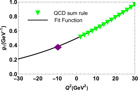
Figure 3: The sum rule’s data and fit function for $g_{1}(Q^{2})$. The diamond fixes the point $Q^{2}=-m_{J/\psi}^{2}$ where $g_{1}$ has been estimated.

III.2 Decay $T\rightarrow\eta_{b}\eta_{c}$

The partial width of the process $T\rightarrow\eta_{b}\eta_{c}$ is determined by the strong coupling $g_{2}$ at the vertex $T\eta_{b}\eta_{c}$. In the framework of the SR method the form factor $g_{2}(q^{2})$ can be obtained from analysis of the correlator

$$\Pi_{\mu\nu}(p,p^{\prime}) = i^{2}\int d^{4}xd^{4}ye^{ip^{\prime}y}e^{-ipx}\langle 0|\mathcal{T}\{\ J^{\eta_{b}}(y)$$ (34)

$$\times J^{\eta_{c}}(0)J_{\mu\nu}^{\dagger}(x)\}|0\rangle.$$

The interpolating currents of the quarkonia $\eta_{c}$ and $\eta_{b}$ in Eq. (34) are

$$J^{\eta_{c}}(x)=\overline{c}_{i}(x)i\gamma_{5}c_{i}(x),\ J^{\eta_{b}}(x)=\overline{b}_{j}(x)i\gamma_{5}b_{j}(x).$$ (35)

The matrix elements necessary to calculate $\Pi_{\mu\nu}^{\mathrm{Phys}}(p,p^{\prime})$ are

$$\langle 0|J^{\eta_{b}}|\eta_{b}(p^{\prime})\rangle=\frac{f_{\eta_{b}}m_{\eta_{b}}^{2}}{2m_{b}},$$

$$\langle 0|J^{\eta_{c}}|\eta_{c}(q)\rangle=\frac{f_{\eta_{c}}m_{\eta_{c}}^{2}}{2m_{c}},$$ (36)

with $f_{\eta_{b}}$, $m_{\eta_{b}}$ and $f_{\eta_{c}}$, $m_{\eta_{c}}$ being the decay constants and masses of the mesons $\eta_{b}$ and $\eta_{c}$, respectively. The vertex $T\eta_{b}\eta_{c}$ is modeled by the expression

$$\langle\eta_{b}(p^{\prime})\eta_{c}(q)|T(p,\epsilon)\rangle=g_{2}(q^{2})\epsilon_{\alpha\beta}^{(\lambda)}(p)p^{\prime\alpha}p^{\prime\beta}.$$ (37)

For the correlator $\Pi_{\mu\nu}^{\mathrm{Phys}}(p,p^{\prime})$, we find

$$\Pi_{\mu\nu}^{\mathrm{Phys}}(p,p^{\prime})=g_{2}(q^{2})\frac{\Lambda f_{\eta_{b}}m_{\eta_{b}}^{2}f_{\eta_{c}}m_{\eta_{c}}^{2}}{4m_{b}m_{c}\left(p^{2}-m^{2}\right)(p^{\prime 2}-m_{\eta_{b}}^{2})}$$

$$\times\frac{1}{(q^{2}-m_{\eta_{c}}^{2})}\left[\frac{m^{4}-2m^{2}(m_{\eta_{b}}^{2}+q^{2})+(m_{\eta_{b}}^{2}-q^{2})^{2}}{12m^{2}}g_{\mu\nu}\right.$$

$$\left.+p_{\mu}^{\prime}p_{\nu}^{\prime}+\text{other terms}\right],$$ (38)

The QCD side of the sum rule $\Pi_{\mu\nu}^{\mathrm{OPE}}(p,p^{\prime})$ has the form

$$\Pi_{\mu\nu}^{\mathrm{OPE}}(p,p^{\prime})=i\int d^{4}xd^{4}ye^{ip^{\prime}y}e^{-ipx}\left\{\mathrm{Tr}\left[\gamma_{5}S_{b}^{ia}(y-x)\right.\right.$$

$$\left.\times\gamma_{\mu}\widetilde{S}_{c}^{jb}(-x)\gamma_{5}\widetilde{S}_{c}^{bj}(x)\gamma_{\nu}S_{b}^{ai}(x-y)\right]$$

$$\left.-\mathrm{Tr}\left[\gamma_{5}S_{b}^{ia}(y-x)\gamma_{\mu}\widetilde{S}_{c}^{jb}(-x)\gamma_{5}\widetilde{S}_{c}^{aj}(x)\gamma_{\nu}S_{b}^{bi}(x-y)\right]\right\}.$$

(39)

The functions $\Pi_{\mu\nu}^{\mathrm{Phys}}(p,p^{\prime})$ and $\Pi_{\mu\nu}^{\mathrm{OPE}}(p,p^{\prime})$ have the same Lorentz organizations. We consider terms $\sim p_{\mu}^{\prime}p_{\nu}^{\prime}$ and use corresponding invariant amplitudes $\Pi_{2}^{\mathrm{Phys}}(p^{2},p^{\prime 2},q^{2})$ and $\Pi_{2}^{\mathrm{OPE}}(p^{2},p^{\prime 2},q^{2})$ to derive the sum rule for the form factor $g_{2}(q^{2})$

$$g_{2}(q^{2})=\frac{4m_{c}m_{b}(q^{2}-m_{\eta_{c}}^{2})}{\Lambda f_{\eta_{c}}m_{\eta_{c}}^{2}f_{\eta_{b}}m_{\eta_{b}}^{2}}e^{m^{2}/M_{1}^{2}}e^{m_{\eta_{b}}^{2}/M_{2}^{2}}$$

$$\times\Pi_{2}(\mathbf{M}^{2},\mathbf{s}_{0},q^{2}),$$ (40)

where $\Pi_{2}(\mathbf{M}^{2},\mathbf{s}_{0},q^{2})$ is the amplitude $\Pi_{2}^{\mathrm{OPE}}(p^{2},p^{\prime 2},q^{2})$ after Borel transformations and continuum subtractions

$$\Pi_{2}(\mathbf{M}^{2},\mathbf{s}_{0},q^{2})=\int_{4\mathcal{M}^{2}}^{s_{0}}ds\int_{4m_{b}^{2}}^{s_{0}^{\prime}}ds^{\prime}\rho_{2}(s,s^{\prime},q^{2})$$

$$\times e^{-s/M_{1}^{2}}e^{-s^{\prime}/M_{2}^{2}}.$$ (41)

Remaining manipulations are usual prescriptions of SR method which have been explained above. In numerical computations, for the masses of the quarkonia $\eta_{c}$ and $\eta_{b}$, we use $m_{\eta_{c}}=(2984.1\pm 0.4)~{}\mathrm{MeV}$, $m_{\eta_{b}}=(9398.7~{}\pm 2.0)\ \mathrm{MeV}\$ from PDG PDG:2022 . The decay constant $f_{\eta_{c}}=(421\pm 35)~{}\mathrm{MeV}$ was extracted from SR analysis Veliev:2010vd , whereas for $f_{\eta_{b}}$ we employ $724~{}\mathrm{MeV}$. We have utilized also the following windows for $M_{2}^{2}$, and $s_{0}^{\prime}$ in the $\eta_{b}$ channel

$$M_{2}^{2}\in[10,12]~{}\mathrm{GeV}^{2},\ s_{0}^{\prime}\in[95,99]~{}\mathrm{GeV}^{2}.$$ (42)

The extrapolating function $\mathcal{G}_{2}(Q^{2})$ and parameters $\mathcal{G}_{2}^{0}=33.63~{}\mathrm{GeV}^{-1}$, $c_{2}^{1}=8.31$, and $c_{2}^{2}=-13.55$ lead to reasonable agreement with SR data. Then the strong coupling $g_{2}$ amounts to

$$g_{2}\equiv\mathcal{G}_{2}(-m_{\eta_{c}}^{2})=(20.4\pm 4.9)\ \mathrm{GeV}^{-1}.$$ (43)

The partial width of this process is equal to

$$\Gamma\left[T\rightarrow\eta_{b}\eta_{c}\right]=g_{2}^{2}\frac{\lambda_{2}}{40\pi m^{2}}|M_{2}|^{2},$$ (44)

where

$$|M_{2}|^{2}=\frac{\left[m^{4}+(m_{\eta_{b}}^{2}-m_{\eta_{c}}^{2})^{2}-2m^{2}(m_{\eta_{b}}^{2}+m_{\eta_{c}}^{2})\right]^{2}}{24m^{4}},$$

(45)

and $\lambda_{2}=\lambda(m,m_{\eta_{b}},m_{\eta_{c}})$.

The width of the decay $T\rightarrow\eta_{b}\eta_{c}$ is

$$\Gamma\left[T\rightarrow\eta_{b}\eta_{c}\right]=(21.1\pm 7.2)~{}\mathrm{MeV}.$$ (46)

IV Modes $T\rightarrow B_{c}^{\ast+}B_{c}^{\ast-}$ and $B_{c}^{+}B_{c}^{-}$

Here, we consider decays of the tensor tetraquark $T$ to $B_{c}^{\ast+}B_{c}^{\ast-}$ and $B_{c}^{+}B_{c}^{-}$ final states. It is known that experimental information about $B_{c}$ mesons is limited by the mass of $B_{c}^{\pm}$ and its first radial excitation $B_{c}^{\pm}(2S)$ PDG:2022 . Therefore, for parameters of the $c\overline{b}$ ($b\overline{c}$) mesons with other spin-parities one should use theoretical predictions. In the case of the vector meson $B_{c}^{\ast\pm}$, for its mass and decay constant we employ

$$m_{B_{c}^{\ast}}=6338~{}\mathrm{MeV},\ f_{B_{c}^{\ast}}=471~{}\mathrm{MeV}$$ (47)

from Refs. Godfrey:2004ya ; Eichten:2019gig , respectively. We also utilize the experimental value $m_{B_{c}}=6274.47(27)(17)~{}\mathrm{MeV}$ for the mass of  $B_{c}^{\pm}$ and decay constant $f_{B_{c}}=(371\pm 37)~{}\mathrm{MeV}$ from Ref. Wang:2024fwc . It is not difficult to see that the processes $T\rightarrow B_{c}^{\ast+}B_{c}^{\ast-}$ and $B_{c}^{+}B_{c}^{-}$ are permitted decay modes of the tensor diquark-antidiquark state $T$, because thresholds for production of the $B_{c}^{\ast+}B_{c}^{\ast-}$ and $B_{c}^{+}B_{c}^{-}$ final-states $12.68~{}\mathrm{GeV}$ and $12.55~{}\mathrm{GeV}$ are below its mass $m$.

IV.1 $T\rightarrow B_{c}^{\ast+}B_{c}^{\ast-}$

Analysis of this decay goes in line with a scheme presented and explained above. Therefore, we write down principal formulas and final results.

The correlation function to derive SR for the form factor $\widetilde{g}_{1}(q^{2})$ responsible for strong interaction at the vertex $TB_{c}^{\ast+}B_{c}^{\ast-}$ is

$$\widetilde{\Pi}_{\mu\nu\alpha\beta}(p,p^{\prime}) = i^{2}\int d^{4}xd^{4}ye^{ip^{\prime}y}e^{-ipx}\langle 0|\mathcal{T}\{J_{\mu}^{B_{c}^{\ast+}}(y)$$ (48)

$$\times J_{\nu}^{B_{c}^{\ast-}}(0)J_{\alpha\beta}^{\dagger}(x)\}|0\rangle.$$

Here, $J_{\mu}^{B_{c}^{\ast+}}$ and $J_{\nu}^{B_{c}^{\ast-}}$ are the interpolating currents of $B_{c}^{\ast+}$ and $B_{c}^{\ast-}$ mesons which are determined by the expressions

$$J_{\mu}^{B_{c}^{\ast+}}(x)=\overline{b}_{i}(x)\gamma_{\mu}c_{i}(x),\ J_{\nu}^{B_{c}^{\ast-}}(x)=\overline{c}_{j}(x)\gamma_{\nu}b_{j}(x).$$ (49)

In terms of the physical parameters of the particles $\widetilde{\Pi}_{\mu\nu\alpha\beta}(p,p^{\prime})$ acquires the following form

$$\widetilde{\Pi}_{\mu\nu\alpha\beta}(p,p^{\prime})=\frac{\langle 0|J_{\mu}^{B_{c}^{\ast+}}|B_{c}^{\ast+}(p^{\prime},\varepsilon_{1})\rangle}{p^{\prime 2}-m_{B_{c}^{\ast}}^{2}}\frac{\langle 0|J_{\nu}^{B_{c}^{\ast-}}|B_{c}^{\ast-}(q,\varepsilon_{2})\rangle}{q^{2}-m_{B_{c}^{\ast}}^{2}}$$

$$\times\langle B_{c}^{\ast+}(p^{\prime},\varepsilon_{1})B_{c}^{\ast-}(q,\varepsilon_{2})|T(p,\epsilon)\rangle\frac{\langle T(p,\epsilon)|J_{\alpha\beta}^{\dagger}|0\rangle}{p^{2}-m^{2}}$$

$$+\cdots.$$ (50)

Subsequent calculations are carried out using the matrix elements

$$\langle 0|J_{\mu}^{B_{c}^{\ast+}}|B_{c}^{\ast+}(p^{\prime},\varepsilon_{1})\rangle=f_{B_{c}^{\ast}}m_{B_{c}^{\ast}}\varepsilon_{1\mu}(p^{\prime}),$$

$$\langle 0|J_{\nu}^{B_{c}^{\ast-}}|B_{c}^{\ast-}(q,\varepsilon_{2})\rangle=f_{B_{c}^{\ast}}m_{B_{c}^{\ast}}\varepsilon_{2\nu}(q),$$ (51)

where $\varepsilon_{1\mu}(p^{\prime})$ and $\varepsilon_{2\nu}(q)$ are the polarization vectors of $B_{c}^{\ast+}$ and $B_{c}^{\ast-}$, respectively. The vertex $TB_{c}^{\ast+}B_{c}^{\ast-}$ is considered in the form Eq. (23) with replacement $g_{1}(q^{2})\rightarrow\widetilde{g}_{1}(q^{2})$.

Then $\widetilde{\Pi}_{\mu\nu\alpha\beta}^{\mathrm{Phys}}(p,p^{\prime})$ in terms of the physical parameters of the tetraquark $T$ and mesons $B_{c}^{\ast\pm}$ reads

$$\widetilde{\Pi}_{\mu\nu\alpha\beta}^{\mathrm{Phys}}(p,p^{\prime})=\frac{\widetilde{g}_{1}(q^{2})\Lambda f_{B_{c}^{\ast}}^{2}m_{B_{c}^{\ast}}^{2}}{\left(p^{2}-m^{2}\right)\left(p^{\prime 2}-m_{B_{c}^{\ast}}^{2}\right)}$$

$$\times\frac{1}{(q^{2}-m_{B_{c}^{\ast}}^{2})}\left[\frac{1}{2}p_{\mu}p_{\alpha}^{\prime}g_{\nu\beta}+\frac{m^{2}+m_{B_{c}^{\ast}}^{2}-q^{2}}{4m^{2}}p_{\mu}^{\prime}p_{\alpha}g_{\beta\nu}\right.$$

$$\left.+p_{\beta}^{\prime}p_{\alpha}^{\prime}g_{\mu\nu}+\text{other structures}\right]+\cdots.$$ (52)

The function $\widetilde{\Pi}_{\mu\nu\alpha\beta}(p,p^{\prime})$ computed in terms of the quark propagators is equal to

$$\widetilde{\Pi}_{\mu\nu\alpha\beta}^{\mathrm{OPE}}(p,p^{\prime})=i\int d^{4}xd^{4}ye^{ip^{\prime}y}e^{-ipx}\left\{\mathrm{Tr}\left[\gamma_{\mu}S_{b}^{ia}(y-x)\right.\right.$$

$$\left.\times\gamma_{\alpha}\widetilde{S}_{c}^{jb}(-x)\gamma_{\nu}\widetilde{S}_{b}^{aj}(x)\gamma_{\beta}S_{c}^{bi}(x-y)\right]$$

$$\left.-\mathrm{Tr}\left[\gamma_{\mu}S_{b}^{ia}(y-x)\gamma_{\alpha}\widetilde{S}_{c}^{jb}(-x)\gamma_{\nu}\widetilde{S}_{b}^{bj}(x)\gamma_{\beta}S_{c}^{ai}(x-y)\right]\right\}.$$

The sum rule for $\widetilde{g}_{1}(q^{2})$ is derived using invariant amplitudes corresponding to terms $\sim p_{\mu}p_{\alpha}^{\prime}g_{\nu\beta}$

$$\widetilde{g}_{1}(q^{2})=\frac{2(q^{2}-m_{\eta_{c}}^{2})}{\Lambda f_{B_{c}^{\ast}}^{2}m_{B_{c}^{\ast}}^{2}}e^{m^{2}/M_{1}^{2}}e^{m_{B_{c}^{\ast}}^{2}/M_{2}^{2}}$$

$$\times\widetilde{\Pi}_{1}(\mathbf{M}^{2},\mathbf{s}_{0},q^{2}),$$ (54)

where $\widetilde{\Pi}_{1}(\mathbf{M}^{2},\mathbf{s}_{0},q^{2})$  is the amplitude $\widetilde{\Pi}_{1}^{\mathrm{OPE}}(p^{2},p^{\prime 2},q^{2})$ obtained after relevant transformations.

Numerical computations have been carried out by employing the following values for the parameters $M_{2}^{2}$ and$\ s_{0}^{\prime}$ in the $B_{c}^{\ast+}$ channel

$$M_{2}^{2}\in[6.5,7.5]~{}\mathrm{GeV}^{2},\ s_{0}^{\prime}\in[49,51]~{}\mathrm{GeV}^{2}.$$ (55)

The fitted constants of the function $\widetilde{\mathcal{G}}_{1}(Q^{2})$ are $\widetilde{\mathcal{G}}_{1}^{0}=0.31~{}\mathrm{GeV}^{-1}$, $\widetilde{c}_{1}^{1}=0.19$, and $\widetilde{c}_{1}^{2}=3.37$. We find for the strong coupling $\widetilde{g}_{1}$

$$\widetilde{g}_{1}\equiv\widetilde{\mathcal{G}}_{1}(-m_{B_{c}^{\ast}}^{2})=(3.6\pm 0.9)\times 10^{-1}\ \mathrm{GeV}^{-1}.$$ (56)

The partial width of the decay $T\rightarrow B_{c}^{\ast+}B_{c}^{\ast-}$ is equal to

$$\Gamma\left[T\rightarrow B_{c}^{\ast+}B_{c}^{\ast-}\right]=\frac{\widetilde{g}_{1}^{2}\widetilde{\lambda}_{1}}{80\pi m^{2}}(m^{4}-3m^{2}m_{B_{c}^{\ast}}^{2}+6m_{B_{c}^{\ast}}^{4}),$$ (57)

where $\widetilde{\lambda}_{1}=\lambda(m,m_{B_{c}^{\ast}},m_{B_{c}^{\ast}})$. Alternatively, the width of this decay can be obtained from Eqs. (30) and (31) upon replacement $m_{J/\psi}=m_{\Upsilon}\rightarrow m_{B_{c}^{\ast}}$.

Numerical calculations yield

$$\Gamma\left[T\rightarrow B_{c}^{\ast+}B_{c}^{\ast-}\right]=(20.1\pm 6.6)~{}\mathrm{MeV}.$$ (58)

IV.2 $T\rightarrow B_{c}^{+}B_{c}^{-}$

The process $T\rightarrow B_{c}^{+}B_{c}^{-}$ is investigated in analogous manner. We consider the correlation function

$$\widetilde{\Pi}_{\mu\nu}(p,p^{\prime}) = i^{2}\int d^{4}xd^{4}ye^{ip^{\prime}y}e^{-ipx}\langle 0|\mathcal{T}\{\ J^{B_{c}^{+}}(y)$$ (59)

$$\times J^{B_{c}^{-}}(0)J_{\mu\nu}^{\dagger}(x)\}|0\rangle.$$

with $\ J^{B_{c}^{+}}(x)$ and $J^{B_{c}^{-}}(x)$ being the interpolating currents of the $B_{c}^{+}$ and $B_{c}^{-}$ mesons

$$\ J^{B_{c}^{+}}(x)=\overline{b}_{i}(x)i\gamma_{5}c_{i}(x),\ J^{B_{c}^{-}}(x)=\overline{c}_{j}(x)i\gamma_{5}b_{j}(x).$$ (60)

The matrix elements of the $B_{c}^{\pm}$ mesons are

$$\langle 0|J^{B_{c}^{\pm}}|B_{c}^{\pm}\rangle=\frac{f_{B_{c}}m_{B_{c}}^{2}}{m_{b}+m_{c}}.$$ (61)

The vertex $\langle B_{c}^{+}(p^{\prime})B_{c}^{-}(q)|T(p,\epsilon)\rangle$ has the form

$$\langle B_{c}^{+}(p^{\prime})B_{c}^{-}(q)|T(p,\epsilon)\rangle=\widetilde{g}_{2}(q^{2})\epsilon_{\alpha\beta}^{(\lambda)}(p)p^{\prime\alpha}p^{\prime\beta}.$$ (62)

The $\widetilde{\Pi}_{\mu\nu}^{\mathrm{Phys}}(p,p^{\prime})$ obtained using these matrix elements after some substitutions [$m_{\eta_{b}}^{2}\mbox{and }m_{\eta_{c}}^{2}\rightarrow m_{B_{c}}^{2}$, $4m_{c}m_{b}\rightarrow(m_{b}+m_{c})^{2}$, etc.] is given by Eq. (38), whereas the QCD side of SR is defined by Eq. (39). The SR for the form factor $\widetilde{g}_{2}(q^{2})$ is

$$\widetilde{g}_{2}(q^{2})=\frac{(m_{b}+m_{c})^{2}(q^{2}-m_{B_{c}}^{2})}{\Lambda f_{B_{c}}^{2}m_{B_{c}}^{4}}e^{m^{2}/M_{1}^{2}}e^{m_{B_{c}}^{2}/M_{2}^{2}}$$

$$\times\widetilde{\Pi}_{2}(\mathbf{M}^{2},\mathbf{s}_{0},q^{2}).$$ (63)

In numerical analysis, we have used the following parameters

$$M_{2}^{2}\in[6.5,7.5]~{}\mathrm{GeV}^{2},\ s_{0}^{\prime}\in[45,47]~{}\mathrm{GeV}^{2}.$$ (64)

Computations of the form factor $\widetilde{g}_{2}(q^{2})$ and coupling $\widetilde{g}_{2}$ lead to the prediction

$$\widetilde{g}_{2}\equiv\widetilde{\mathcal{G}}_{2}(-m_{B_{c}}^{2})=(26.6\pm 6.4)\ \mathrm{GeV}^{-1},$$ (65)

where $\widetilde{\mathcal{G}}_{2}(Q^{2})$ is the fitting function with parameters $\widetilde{\mathcal{G}}_{2}^{0}=29.89~{}\mathrm{GeV}^{-1}$, $\widetilde{c}_{2}^{1}=0.95$, and $\widetilde{c}_{2}^{2}=1.90$.

The width of the decay $T\rightarrow B_{c}^{+}B_{c}^{-}$ can be computed by means of the expression

$$\Gamma\left[T\rightarrow B_{c}^{+}B_{c}^{-}\right]=\widetilde{g}_{2}^{2}\frac{\widetilde{\lambda}_{2}}{960\pi m^{2}}\left(m^{2}-4m_{B_{c}}^{2}\right)^{2},$$ (66)

where $\widetilde{\lambda}_{2}=\lambda(m,m_{B_{c}},m_{B_{c}})$. This formula in the limit $m_{\eta_{b}}\mbox{and }m_{\eta_{c}}\rightarrow m_{B_{c}}$ can be obtained from Eq. (45). Our computations yield

$$\Gamma\left[T\rightarrow B_{c}^{+}B_{c}^{-}\right]=(20.1\pm 6.9)~{}\mathrm{MeV}.$$ (67)

V Decays due to $b\overline{b}$ annihilations

As it has been emphasized above, the tetraquark $T$ may transform to a conventional meson pair also due to annihilation of $b\overline{b}$ to light quark-antiquark pairs Becchi:2020mjz ; Becchi:2020uvq ; Agaev:2023ara and creation of $DD$ mesons with required electric charges and spin-parities. Here, we consider decays of the tetraquark $T$ to $D^{\ast 0}\overline{D}^{\ast 0}$, $D^{0}\overline{D}^{0}$, $D^{\ast+}D^{\ast-}$, and $D^{+}D^{-}$ mesons.

It is clear that these decays are kinematically possible modes for transformation of the tetraquark $T$ to ordinary mesons. We study these processes in the same context of the three-point sum rule approach. But here we encounter a situation when relevant correlation functions contain$\ \overline{b}b$ quarks’ vacuum matrix element $\langle\overline{b}b\rangle$ Agaev:2023ara . In calculations, we replace this matrix element with known value of the gluon condensate $\langle\alpha_{s}G^{2}/\pi\rangle$.

V.1 Decays $T\rightarrow D^{\ast 0}\overline{D}^{\ast 0}$ and $D^{0}\overline{D}^{0}$

Let us analyze in the process $T\rightarrow D^{\ast 0}\overline{D}^{\ast 0}$. To find the coupling $G_{1}$ of particles at the vertex $TD^{\ast 0}\overline{D}^{\ast 0}$, we start from the correlation function

$$\widehat{\Pi}_{\mu\nu\alpha\beta}(p,p^{\prime}) = i^{2}\int d^{4}xd^{4}ye^{ip^{\prime}y}e^{-ipx}\langle 0|\mathcal{T}\{J_{\mu}^{\overline{D}^{\ast 0}}(y)$$ (68)

$$\times J_{\nu}^{D^{\ast 0}}(0)J_{\alpha\beta}^{\dagger}(x)\}|0\rangle,$$

where $J_{\mu}^{\overline{D}^{\ast 0}}(x)$ and $J_{\nu}^{D^{\ast 0}}(x)$ are interpolating currents for the mesons $\overline{D}^{\ast 0}$ and $D^{\ast 0}$

$$J_{\mu}^{\overline{D}^{\ast 0}}(x)=\overline{c}_{i}(x)\gamma_{\mu}u_{i}(x),\text{ }J_{\nu}^{D^{\ast 0}}(x)=\overline{u}_{j}(x)\gamma_{\nu}c_{j}(x).$$ (69)

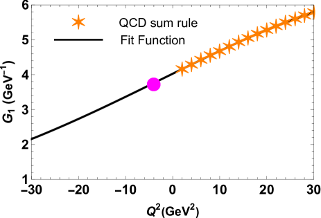
Figure 4: The sum rule data and extrapolating function for the form factor $G_{1}(Q^{2})$. The circle shows the point $Q^{2}=-m_{D^{\ast 0}}^{2}$.

The expression of the function $\widehat{\Pi}_{\mu\nu\alpha\beta}(p,p^{\prime})$ in terms of $T$, $D^{\ast 0}$, and $\overline{D}^{\ast 0}$ particles’ parameters reads

$$\widehat{\Pi}_{\mu\nu\alpha\beta}^{\mathrm{Phys}}(p,p^{\prime})=\frac{\langle 0|J_{\mu}^{\overline{D}^{\ast 0}}|\overline{D}^{\ast 0}(p^{\prime},\varepsilon_{1})\rangle}{p^{\prime 2}-m_{D^{\ast 0}}^{2}}\frac{\langle 0|J_{\nu}^{D^{\ast 0}}|D^{\ast 0}(q,\varepsilon_{2})\rangle}{q^{2}-m_{D^{\ast 0}}^{2}}$$

$$\times\langle\overline{D}^{\ast 0}(p^{\prime},\varepsilon_{1})D^{\ast 0}(q,\varepsilon_{2})|T(p,\epsilon)\rangle\frac{\langle T(p,\epsilon)|J_{\mu}^{\dagger}|0\rangle}{p^{2}-m^{2}}+\cdots,$$

where $m_{D^{\ast 0}}=(2006.85\pm 0.05)~{}\mathrm{MeV}$ is the mass of the mesons $\overline{D}^{\ast 0}$ and $D^{\ast 0}$, whereas $\varepsilon_{1\mu}$ and $\varepsilon_{2\nu}$ are their polarization vectors.

The matrix elements which are required to calculate $\widehat{\Pi}_{\mu\nu\alpha\beta}^{\mathrm{Phys}}(p,p^{\prime})$ are

$$\langle 0|J_{\mu}^{\overline{D}^{\ast 0}}|\overline{D}^{\ast 0}(p^{\prime},\varepsilon_{1})\rangle = f_{D^{\ast}}m_{D^{\ast 0}}\varepsilon_{1\mu}(p^{\prime}),$$

$$\langle 0|J_{\nu}^{D^{\ast 0}}|D^{\ast 0}(q,\varepsilon_{2})\rangle = f_{D^{\ast}}m_{D^{\ast 0}}\varepsilon_{2\nu}(q),$$ (71)

with $f_{D^{\ast}}=(252.2\pm 22.66)~{}\mathrm{MeV}$ being the decay constant of the mesons $D^{\ast 0}$ and $\overline{D}_{D}^{\ast 0}$. The vertex $\langle\overline{D}^{\ast 0}(p^{\prime},\varepsilon_{1})D^{\ast 0}(q,\varepsilon_{2})|T(p,\epsilon)\rangle$ is modeled in the form of Eq. (23).

The correlator $\widehat{\Pi}_{\mu\nu\alpha\beta}^{\mathrm{Phys}}(p,p^{\prime})$ is a sum of different components. The SR for the form factor $G_{1}(q^{2})$ is obtained by employing the invariant amplitude $\widehat{\Pi}_{1}^{\mathrm{Phys}}(p^{2},p^{\prime 2},q^{2})$ that corresponds to the structure $p_{\mu}p_{\alpha}^{\prime}g_{\beta\nu}$. The same correlation function $\widehat{\Pi}_{\mu\nu\alpha\beta}(p,p^{\prime})$ computed using the heavy and light quark propagators is

$$\widehat{\Pi}_{\mu\nu\alpha\beta}^{\mathrm{OPE}}(p,p^{\prime})=\frac{2}{3}\langle\overline{b}b\rangle\int d^{4}xd^{4}ye^{ip^{\prime}y}e^{-ipx}$$

$$\times\mathrm{Tr}\left[\gamma_{\mu}S_{u}^{ij}(y)\gamma_{\nu}{}S_{c}^{jb}(-x)\gamma_{\alpha}\gamma_{\beta}S_{c}^{bi}(x-y)\right],$$ (72)

where $S_{u}(x)$ is the propagator of $u$ quark Agaev:2020zad .

For further studies, we make use of the relation between condensates

$$\langle\overline{b}b\rangle=-\frac{1}{12\pi m_{b}}\langle\frac{\alpha_{s}G^{2}}{\pi}\rangle.$$ (73)

In what follows, we denote by $\widehat{\Pi}_{1}^{\mathrm{OPE}}(p^{2},p^{\prime 2},q^{2})$ the invariant amplitude which corresponds in $\widehat{\Pi}_{\mu\nu\alpha\beta}^{\mathrm{OPE}}(p,p^{\prime})$ to the term $p_{\mu}p_{\alpha}^{\prime}g_{\beta\nu}$.

The SR for the coupling $G_{1}(q^{2})$ reads

$$G_{1}(q^{2})=\frac{2(q^{2}-m_{D^{\ast 0}}^{2})}{\Lambda f_{D^{\ast}}^{2}m_{D^{\ast 0}}^{2}}e^{m^{2}/M_{1}^{2}}e^{m_{D^{\ast 0}}^{2}/M_{2}^{2}}$$

$$\times\widehat{\Pi}_{1}(\mathbf{M}^{2},\mathbf{s}_{0},q^{2}),$$ (74)

where $\widehat{\Pi}_{1}(\mathbf{M}^{2},\mathbf{s}_{0},q^{2})$ is the amplitude $\widehat{\Pi}_{1}^{\mathrm{OPE}}(p^{2},p^{\prime 2},q^{2})$ undergone to Borel transformations and continuum subtractions.

To extract $G_{1}(q^{2})$ from this SR we carry out standard manipulations, and skip further details: In the $\overline{D}^{\ast 0}$ meson channel, we have used the parameters

$$M_{2}^{2}\in[2,3]~{}\mathrm{GeV}^{2},\ s_{0}^{\prime}\in[5.7,5.8]~{}\mathrm{GeV}^{2}.$$ (75)

The coupling $G_{1}$ has been evaluated by employing SR data for $Q^{2}=2-30\ \mathrm{GeV}^{2}$ and extrapolating function with parameters $\widehat{\mathcal{G}}_{1}^{0}=0.04~{}\mathrm{GeV}^{-1}$, $\widehat{c}_{1}^{1}=2.66$, and $\widehat{c}_{1}^{2}=-3.79$. The SR data and fit function $\widehat{\mathcal{G}}_{1}(Q^{2})$ are plotted in Fig. 4. The coupling $G_{1}$ has been computed at the mass shell $q^{2}=m_{D^{\ast 0}}^{2}$ and amounts to

$$G_{1}\equiv\widehat{\mathcal{G}}_{1}(-m_{D^{\ast 0}}^{2})=(3.76\pm 0.90)\times 10^{-2}\ \mathrm{GeV}^{-1}.$$ (76)

The width of the decay $T\rightarrow D^{\ast 0}\overline{D}^{\ast 0}$ is

$$\Gamma\left[T\rightarrow D^{\ast 0}\overline{D}^{\ast 0}\right]=(5.1\pm 1.7)~{}\mathrm{MeV}.$$ (77)

The second process $T\rightarrow D^{0}\overline{D}^{0}$ is considered starting from the correlator

$$\widehat{\Pi}_{\mu\nu}(p,p^{\prime}) = i^{2}\int d^{4}xd^{4}ye^{ip^{\prime}y}e^{-ipx}\langle 0|\mathcal{T}\{J^{\overline{D}^{0}}(y)$$ (78)

$$\times J^{D^{0}}(0)J_{\mu\nu}^{\dagger}(x)\}|0\rangle,$$

where the currents $J^{\overline{D}^{0}}(x)$ and $J^{D^{0}}(x)$ are defined by expressions

$$J^{\overline{D}^{0}}(x)=\overline{c}_{i}(x)i\gamma_{5}u_{i}(x),\text{ }J^{D^{0}}(x)=\overline{u}_{j}(x)i\gamma_{5}c_{j}(x).$$ (79)

To get the sum rule for the form factor $G_{2}(q^{2})$ responsible for strong interaction of particles at the vertex $TD^{0}\overline{D}^{0}$, we calculate $\widehat{\Pi}_{\mu\nu}^{\mathrm{Phys}}(p,p^{\prime})$ and $\widehat{\Pi}_{\mu\nu}^{\mathrm{OPE}}(p,p^{\prime})$.

We determine $\widehat{\Pi}_{\mu\nu}^{\mathrm{Phys}}(p,p^{\prime})$ using the following matrix elements

$$\langle 0|J^{\overline{D}^{0}}|\overline{D}^{0}\rangle=\langle 0|J^{D^{0}}|D^{0}\rangle=\frac{f_{D}m_{D^{0}}^{2}}{m_{c}},$$ (80)

and

$$\langle\overline{D}^{0}(p^{\prime})D^{0}(q)|T(p,\epsilon)\rangle=G_{2}(q^{2})\epsilon_{\alpha\beta}^{(\lambda)}(p)p^{\prime\alpha}p^{\prime\beta},$$ (81)

with $m_{D^{0}}=(1864.84\pm 0.05)~{}\mathrm{MeV}$ and $f_{D}=(211.9\pm 1.1)~{}\mathrm{MeV}$ being the mass and decay constant of mesons $D^{0}$ and $\overline{D}^{0}$ PDG:2022 ; Rosner:2015wva . As a result, we obtain

$$\widehat{\Pi}_{\mu\nu}^{\mathrm{Phys}}(p,p^{\prime})=\frac{G_{2}(q^{2})\Lambda f_{D}^{2}m_{D^{0}}^{4}}{m_{c}^{2}\left(p^{2}-m^{2}\right)\left(p^{\prime 2}-m_{D^{0}}^{2}\right)\left(q^{2}-m_{D^{0}}^{2}\right)}$$

$$\times\left[\frac{m^{4}-2m^{2}(m_{D^{0}}^{2}+q^{2})+(m_{D^{0}}^{2}-q^{2})^{2}}{12m^{2}}g_{\mu\nu}\right.$$

$$\left.+p_{\mu}^{\prime}p_{\nu}^{\prime}-\frac{m^{2}+m_{D^{0}}^{2}-q^{2}}{2m^{2}}p_{\mu}p_{\nu}^{\prime}+\text{other terms}\right].$$ (82)

For $\widehat{\Pi}_{\mu\nu}^{\mathrm{OPE}}(p,p^{\prime})$, we find

$$\widehat{\Pi}_{\mu\nu}^{\mathrm{OPE}}(p,p^{\prime})=\frac{2}{3}\langle\overline{b}b\rangle\int d^{4}xd^{4}ye^{ip^{\prime}y}e^{-ipx}$$

$$\times\mathrm{Tr}\left[\gamma_{5}S_{u}^{ij}(y){}\gamma_{5}S_{c}^{jb}(-x)\gamma_{\mu}\gamma_{\nu}S_{c}^{bi}(x-y)\right].$$ (83)

We extract SR for $G_{2}(q^{2})$ using the amplitudes $\widehat{\Pi}_{2}^{\mathrm{Phys}}(p^{2},p^{\prime 2},q^{2})$ and $\widehat{\Pi}_{2}^{\mathrm{OPE}}(p^{2},p^{\prime 2},q^{2})$ corresponding to structures $p_{\mu}^{\prime}p_{\nu}^{\prime}$ and get

$$G_{2}(q^{2})=\frac{m_{c}^{2}(q^{2}-m_{D^{0}}^{2})}{\Lambda f_{D}^{2}m_{D^{0}}^{4}}e^{m^{2}/M_{1}^{2}}e^{m_{D^{0}}^{2}/M_{2}^{2}}$$

$$\times\widehat{\Pi}_{2}(\mathbf{M}^{2},\mathbf{s}_{0},q^{2}),$$ (84)

with $\widehat{\Pi}_{2}(\mathbf{M}^{2},\mathbf{s}_{0},q^{2})$ being the transformed function $\widehat{\Pi}_{2}^{\mathrm{OPE}}(p^{2},p^{\prime 2},q^{2})$.

In numerical calculations we employed the parameters

$$M_{2}^{2}\in[1.5,3]~{}\mathrm{GeV}^{2},\ s_{0}^{\prime}\in[5,5.2]~{}\mathrm{GeV}^{2}.$$ (85)

We have found the coupling $G_{2}$ by means of the of the function $\widehat{\mathcal{G}}_{2}(Q^{2})$ with $\widehat{\mathcal{G}}_{2}^{0}=0.14~{}\mathrm{GeV}^{-1}$, $\widehat{c}_{2}^{1}=2.11$, and $\widehat{c}_{2}^{2}=-3.65$

$$G_{2}\equiv\widehat{\mathcal{G}}_{2}(-m_{D^{0}}^{2})=(0.13\pm 0.03)\ \mathrm{GeV}^{-1}.$$ (86)

The partial width of the decay $T\rightarrow D^{0}\overline{D}^{0}$ is equal to

$$\Gamma\left[T\rightarrow D^{0}\overline{D}^{0}\right]=(4.6\pm 1.5)~{}\mathrm{MeV}.$$ (87)

V.2 Processes $T\rightarrow D^{\ast+}D^{\ast-}$ and $D^{+}D^{-}$

The modes $T\rightarrow D^{\ast+}D^{\ast-}$ and $D^{+}D^{-}$ are explored in accordance with the scheme explained above. Let us study the process $T\rightarrow D^{\ast+}D^{\ast-}$. The strong form factor $G_{3}(q^{2})$ at the vertex $TD^{\ast+}D^{\ast-}$ is extracted from the correlation function

$$\Pi_{\mu\nu\alpha\beta}^{\prime}(p,p^{\prime}) = i^{2}\int d^{4}xd^{4}ye^{ip^{\prime}y}e^{-ipx}\langle 0|\mathcal{T}\{J_{\mu}^{D^{\ast+}}(y)$$ (88)

$$\times J_{\nu}^{D^{\ast-}}(0)J_{\alpha\beta}^{\dagger}(x)\}|0\rangle,$$

where currents for the mesons $D^{\ast+}$ and $D^{\ast-}$ are given by the formulas

$$J_{\mu}^{D^{\ast+}}(x)=\overline{d}_{i}(x)\gamma_{\mu}c_{i}(x),\ J_{\nu}^{D^{\ast-}}(x)=\overline{d}_{j}(x)\gamma_{\nu}d_{j}(x).$$ (89)

The matrix elements of these particles and the vertex are similar to ones introduced above. Therefore, we omit these expressions and write down the QCD side of the SR

$$\overline{\Pi}_{\mu\nu\alpha\beta}^{\prime\mathrm{OPE}}(p,p^{\prime})=-\frac{i}{18m_{b}\pi}\langle\frac{\alpha_{s}G^{2}}{\pi}\rangle\int d^{4}xd^{4}ye^{ip^{\prime}y}e^{-ipx}$$

$$\times\mathrm{Tr}\left[\gamma_{\mu}S_{d}^{ij}(y)\gamma_{\nu}{}S_{c}^{jb}(-x)\gamma_{\alpha}\gamma_{\beta}S_{c}^{bj}(x-y)\right].$$ (90)

As usual, we utilize invariant amplitudes corresponding to the structure $p_{\mu}p_{\alpha}^{\prime}g_{\beta\nu}$. In numerical calculations the Borel and continuum subtraction parameters in the $D^{\ast+}$ channel are fixed as in Eq. (75). The mass of $D^{\ast\pm}$ mesons is $m_{D^{\ast}}=(2010.26\pm 0.05)~{}\mathrm{MeV}$, whereas for their decay constants we use $f_{D^{\ast}}=(252.2\pm 22.66)~{}\mathrm{MeV}$.

The function $\widehat{\mathcal{G}}_{3}(Q^{2})$ with the constants $\widehat{\mathcal{G}}_{3}^{0}=0.04~{}\mathrm{GeV}^{-1}$, $\widehat{c}_{3}^{1}=2.65$, and $\widehat{c}_{3}^{2}=-3.78$ gives to coupling $G_{3}$

$$G_{3}\equiv\widehat{\mathcal{G}}_{3}(-m_{D^{\ast}}^{2})=(3.77\pm 0.90)\times 10^{-2}\ \mathrm{GeV}^{-1}.$$ (91)

For the partial width of the mode $T\rightarrow D^{\ast+}D^{\ast-}$, we get

$$\Gamma\left[T\rightarrow D^{\ast+}D^{\ast-}\right]=(5.1\pm 1.6)~{}\mathrm{MeV}.$$ (92)

The process $T\rightarrow D^{+}D^{-}$ is explored in similar way. The coupling $G_{4}$ responsible for strong interaction of the particles at the vertex $TD^{+}D^{-}$ is

$$G_{4}\equiv\widetilde{\mathcal{G}}_{4}(-m_{D}^{2})=(0.13\pm 0.03)~{}\mathrm{GeV}^{-1}.$$ (93)

For the width of this decay, we find

$$\Gamma\left[T\rightarrow D^{+}D^{-}\right]=(4.6\pm 1.5)~{}\mathrm{MeV}.$$ (94)

Computations performed in present paper permit us to estimate the full width of the axial-vector tetraquark $T$ with content $bc\overline{b}\overline{c}$. As a result, we obtain

$$\Gamma\left[T\right]=(108.4\pm 15.4)~{}\mathrm{MeV}.$$ (95)

VI Conclusions

In present article, we have calculated the mass and full width of the tensor tetraquark  $bc\overline{b}\overline{c}$. Analyses have been performed in the framework of QCD sum rule method. To evaluate the mass of $T$, we have applied the two-point SR method, whereas its decays have been studied by invoking the three-point SR approach.

The mass $m$ of the tensor tetraquark $T$ was evaluated in different articles, sometimes with contradictory results Faustov:2022mvs ; Wu:2016vtq ; Liu:2019zuc ; Chen:2019vrj ; Bedolla:2019zwg ; Cordillo:2020sgc ; Weng:2020jao ; Yang:2021zrc . Our result $m=(12.70\pm 0.09)~{}\mathrm{GeV}$ is smaller than those reported in publications Faustov:2022mvs ; Wu:2016vtq ; Liu:2019zuc ; Chen:2019vrj . In Refs. Bedolla:2019zwg ; Cordillo:2020sgc ; Weng:2020jao ; Yang:2021zrc the authors found the mass of this state in most of cases below $m$. Thus, $m$ evaluated here is somewhere between these two groups of predictions.

The results of current paper demonstrate that the tensor state $T$ can decay to ordinary mesons through strong fall-apart mechanism. In almost all articles cited above authors made similar conclusions: Only in Ref. Yang:2021zrc $T$ was predicted to be stable against two-meson strong dissociations. But let us emphasize that structures $bc\overline{b}\overline{c}$, due to $b\overline{b}$ and $c\overline{c}$ annihilations and generations of ordinary heavy-light mesons, are always strong-interaction unstable particles.

We have calculated partial widths of four processes $T\rightarrow J/\psi\Upsilon$, $\eta_{b}\eta_{c}$ and $B_{c}^{(\ast)+}B_{c}^{(\ast)-}$ which are dominant decay channels of $T$. We have evaluated also widths of modes triggered by $b\overline{b}$ annihilations inside of $T$ and containing at the final states $D^{(\ast)+}D^{(\ast)-}$ and $D^{(\ast)0}\overline{D}^{(\ast)0}$ mesons. It is worth noting that contribution of these processes is not small and forms approximately $18\%$ of the $T$ tetraquark’s full width.

Our predictions characterize $T$ as a wide diquark-antidiquark state, which can decay to two-meson final states through both fall-apart and $b\overline{b}$ annihilation mechanisms. The tensor tetraquark $T$ , as well as the scalar and axial-vector tetraquarks establish a family of fully heavy exotic mesons $bc\overline{b}\overline{c}$ with different spin-parities. Having compared $m$ with masses of the scalar and axial-vector states $m_{\mathrm{S}}=(12.697\pm 0.090)~{}\mathrm{GeV}$ and $m_{\mathrm{AV}}=(12.715\pm 0.090)~{}\mathrm{GeV}$ Agaev:2024wvp ; Agaev:2024mng , one sees that they form almost degenerate system of particles.

Heavy tetraquarks are inseparable part of the exotic hadron spectroscopy. Structures $bc\overline{b}\overline{c}$ were not observed yet, but they can be seen in the future runs of the LHC and Future Circular Collider Carvalho:2015nqf ; Abreu:2023wwg . Publications devoted to fully heavy four-quark states are concentrated on analysis of their masses. Decays of these states, including $bc\overline{b}\overline{c}$ ones, did not become objects of detailed investigations. But besides masses, all conclusions about nature of discovered resonances have to be also based on knowledge about their decay channels and widths: This information is required for reliable interpretation of collected data and planning new measurements.

References

- (1) R. Aaij et al. (LHCb Collaboration), Sci. Bull. 65, 1983 (2020).
- (2) E. Bouhova-Thacker (ATLAS Collaboration), PoS ICHEP2022, 806 (2022).
- (3) A. Hayrapetyan, et al. (CMS Collaboration) Phys. Rev. Lett. 132, 111901 (2024).
- (4) J. R. Zhang, Phys. Rev. D 103, 014018 (2021).
- (5) R. M. Albuquerque, S. Narison, A. Rabemananjara, D. Rabetiarivony, and G. Randriamanatrika, Phys. Rev. D 102, 094001 (2020).
- (6) B. C. Yang, L. Tang, and C. F. Qiao, Eur. Phys. J. C 81, 324 (2021).
- (7) C. Becchi, A. Giachino, L. Maiani, and E. Santopinto, Phys. Lett. B 806, 135495 (2020).
- (8) C. Becchi, A. Giachino, L. Maiani, and E. Santopinto, Phys. Lett. B 811, 135952 (2020).
- (9) Z. G. Wang, Nucl. Phys. B 985, 115983 (2022).
- (10) R. N. Faustov, V. O. Galkin, and E. M. Savchenko, Symmetry 14, 2504 (2022).
- (11) P. Niu, Z. Zhang, Q. Wang, and M. L. Du, Sci. Bull. 68, 800 (2023).
- (12) W. C. Dong and Z. G. Wang, Phys. Rev. D 107, 074010 (2023).
- (13) G. L. Yu, Z. Y. Li, Z. G. Wang, J. Lu, and M. Yan, Eur. Phys. J. C 83, 416 (2023).
- (14) S. Q. Kuang, Q. Zhou, D. Guo, Q. H. Yang, and L. Y. Dai, Eur. Phys. J. C 83, 383 (2023).
- (15) Z. G. Wang and X. S. Yang, AAPPS Bull. 34, 5 (2024).
- (16) X. K. Dong, V. Baru, F. K. Guo, C. Hanhart, and A. Nefediev, Phys. Rev. Lett. 126, 132001 (2021); 127, 119901(E) (2021).
- (17) Z. R. Liang, X. Y. Wu, and D. L. Yao, Phys. Rev. D 104, 034034 (2021).
- (18) S. S. Agaev, K. Azizi, B. Barsbay, and H. Sundu, Phys. Lett. B 844, 138089 (2023).
- (19) S. S. Agaev, K. Azizi, B. Barsbay and H. Sundu, Eur. Phys. J. Plus 138, 935 (2023).
- (20) S. S. Agaev, K. Azizi, B. Barsbay and H. Sundu, Nucl. Phys. A 844, 122768 (2024).
- (21) S. S. Agaev, K. Azizi, B. Barsbay and H. Sundu, Eur. Phys. J. C 83, 994 (2023).
- (22) F. Carvalho, E. R. Cazaroto, V. P. Gonsalves, and F. S. Navarra, Phys. Rev. D 93, 034004 (2016).
- (23) L. M. Abreu, F. Carvalho, J. V. C. Cerquera, and V. P. Goncalves, Eur. Phys. J. C 84, 470 (2024).
- (24) J. Wu, Y. R. Liu, K. Chen, X. Liu, and S. L. Zhu, Phys. Rev. D 97, 094015 (2018).
- (25) M. S. Liu, Q. F. Lü, X. H. Zhang, and Q. Zhao, Phys. Rev. D 100, 016006 (2019).
- (26) X. Chen, Phys. Rev. D 100, 094009 (2019).
- (27) M. A. Bedolla, J. Ferretti, C. D. Roberts, and E. Santopinto Eur. Phys. J. C 80, 1004 (2020).
- (28) M. C. Gordillo, F. De Soto, and J. Segovia Phys. Rev. D 102, 114007 (2020).
- (29) X. Z. Weng, X. L. Chen, W. Z. Deng, and S. L. Zhu Phys. Rev. D 103, 034001 (2021).
- (30) Z. H. Yang, Q. N. Wang, W. Chen, and H. X. Chen Phys. Rev. D 104, 014003 (2021).
- (31) J. Hoffer, G. Eichmann, C. S. Fischer, Phys. Rev. D 109, 074025 (2024).
- (32) S. S. Agaev, K. Azizi, and H. Sundu, Phys. Lett. B 858, 139042 (2024).
- (33) S. S. Agaev, K. Azizi, and H. Sundu, arXiv:2410.00575 [hep-ph].
- (34) M. A. Shifman, A. I. Vainshtein and V. I. Zakharov, Nucl. Phys. B 147, 385 (1979).
- (35) M. A. Shifman, A. I. Vainshtein and V. I. Zakharov, Nucl. Phys. B 147, 448 (1979).
- (36) R. L. Workman et al. [Particle Data Group], Prog. Theor. Exp. Phys. 2022, 083C01 (2022).
- (37) O. Lakhina, and E. S. Swanson, Phys. Rev. D 74, 014012 (2006).
- (38) V. M. Braun, and N. Kivel, Phys. Lett. B 501, 48 (2001).
- (39) T. M. Aliev, and M. Savcı, Phys. Rev. D 99, 015020 (2019).
- (40) S. S. Agaev, K. Azizi, and H. Sundu, Phys. Lett. B 856, 138886 (2024).
- (41) E. V. Veliev, K. Azizi, H. Sundu, and N. Aksit, J. Phys. G 39, 015002 (2012).
- (42) S. Godfrey, Phys. Rev. D 70, 054017 (2004).
- (43) E. J. Eichten, and C. Quigg, Phys. Rev. D 99, 054025 (2019).
- (44) Z. G. Wang, Chin. Phys. C 48, 103104 (2024).
- (45) S. S. Agaev, K. Azizi, B. Barsbay, and H. Sundu, Phys. Rev. D 109, 014006 (2024).
- (46) S. S. Agaev, K. Azizi and H. Sundu, Turk. J. Phys. 44, 95 (2020).
- (47) J. L. Rosner, S. Stone, and R. S. Van de Water,(2015) arXiv:1509.02220.