Quantum permutation puzzles with indistinguishable particles
Abstract
Permutation puzzles, such as the Rubik’s cube and the 15 puzzle, are enjoyed by the general public and mathematicians alike. Here we introduce quantum versions of permutation puzzles where the pieces of the puzzles are replaced with indistinguishable quantum particles. The moves in the puzzle are achieved by swapping or permuting the particles. We show that simply permuting the particles can be mapped to a classical permutation puzzle, even though the identical particles are entangled. However, we obtain a genuine quantum puzzle by adding a quantum move—the square root of SWAP. The resulting puzzle cannot be mapped to a classical permutation puzzle. We focus predominately on the quantization of the slide puzzle and briefly treat the Rubik’s cube.
I Introduction
Permutation puzzles [1], such as the Rubik’s cube and the 15-puzzle, involve scrambling the pieces, with the objective of returning the puzzle to its original arrangement. All of these puzzles are solved by permuting the pieces in groups determined by the connectivity of the puzzle. For the Rubik’s cube, the basic permutation is a rotation about a face. For the 15-puzzle—an example of a “slide puzzle”—the basic permutation is swapping or sliding a piece into the location of a hole; see LABEL:fig:clas_perm_puzz. Our goal is to develop quantum versions of these puzzles.
Previous quantum computing research has linked the Rubik’s cube to quantum walks for encryption [2], scrambling in many-body dynamics [3], Clifford gate synthesis [4], energy-level diagrams [5], and nonlocal entangled states for quantum secret sharing [6]. Additionally, Corli et al. [7] used reinforcement learning to solve the classical cube by embedding its group into a boson-fermion model. Similarly, the 15 puzzle has received attention due to it’s relationship to itinerant ferromagnetism [8]. These analogies are useful for understanding and explaining deep results. However, our goal is to create a family of quantum puzzles whose primary purpose is quantized entertainment.
In this article, we construct quantum puzzles inspired by slide puzzles and the Rubik’s cube. To make a quantum puzzle, we will replace the pieces with quantum particles. A single species of identical particles [9, 10] will replace all the blue pieces and so on for all the other colors. All particles of the same “color” will be indistinguishable from one another, but all particles of different colors will be distinguishable. As the pieces are permuted, we must correctly account for the exchange statistics of the identical particles.
We focus on a 2D version of a permutation puzzle with identical particles, that is related to the 15 puzzle. We show in Section II that replacing pieces with quantum particles results in a new effectively classical puzzle that is finite-dimensional. Fortunately, the quantum structure of the puzzle permits new actions that are not possible classically. In Section III we add a new move, a square root SWAP, which allows the state of the puzzle to leave the subspace of classically allowed states. Then in Section IV we investigate solving strategies and compare how a solver with access to square root SWAPs can outperform solvers with only classical actions. We then consider several extensions to the puzzle. First, in Section V we explore adding more moves to allow our puzzle to, in principle, reach all states in the puzzle Hilbert space. Second, in Section VI we consider larger puzzles with more particles. Third, in Section VII we demonstrate how to generalize our 2D puzzle to 3D with a specific example of the Cube puzzle. Finally, we conclude with some open questions in Section VIII.
II Permutation Puzzles
Consider the following classical slide–like puzzle with two blue tiles and two green tiles
| (1) |
Here, the colored tiles are labelled 1,2,3,4 so they are distinguishable. The most basic operation in permutation puzzles is some method of permuting the pieces. For the slide puzzle, these permutations take the form of sliding a piece into a hole. The first departure of our puzzle from a regular slide puzzle is that we do not require a missing piece, instead we allow the swapping of pieces. In particular, we allow the following SWAP moves
| (2) | ||||
however we do not allow SWAPs between diagonal elements. Given these actions, it is easy to compute that there are arrangements of the board.
Next, we remove the labels to make a stronger analogy with identical particles. However, we insist that the puzzle respects orientation in the same way that most slide puzzles do. This means that rotating the board is not an allowed action, e.g. a rotation about the center
| (not allowed) . | (3) |
When this is taken into account and when the labels are removed there are now unique board states:
| (4) |
It is also clear that using the actions in Eq. 2, any board state can be generated from any other board state.
With the classical board understood we will replace the classical tiles with identical quantum particles. These particles could be sets of identical fermions or bosons. We are interested in the possible unique states of four particles on the board. Two of the particles are green and two are blue. The blue and green particles are distinguishable from each other. But particles with the same color are indistinguishable.
We denote the solved state of the quantum puzzle as
| (5) |
Because some of the particles are identical we must symmetrize or anti-symmetrize the particles, for this reason we momentarily re-introduce particle labels. For identical fermions or bosons the appropriately symmetrized solved state, up to normalization, is
| (6a) | |||||||||||
| (6b) | |||||||||||
In representing the identical particles this way we have assumed that the board is represented in two spatial dimensions and each lattice site of the board contains a single quantum particle. Further, we require that the spatial wavefunctions of these particles are localized to each site so that there is no spatial overlap between the wavefunctions of particles in different sites. From now on we drop the fictitious particle labels, but it should be understood that the underlying wavefunctions for any board state have been (anti) symmetrized.
To determine the quantum state space of the puzzle we start with the solved state and SWAP particles using the operations in Eq. 2. Because these operations are now acting on a quantum state they must be represented by a unitary operator
| (7) |
where denotes a “Up” SWAP, and similarly for Down, Right, and Left. Swapping indistinguishable particles leds to a global phase and thus is a trivial operation e.g.
| (8) |
Instead if we perform a Left SWAP
| (9) |
then the puzzle transitions to a new board state. It is easy to show that the new board state is orthogonal to the solved state, i.e.
| (10) |
by computing overlaps between the underlying (anti) symmetrized wavefunctions, see Appendix A. By applying sequences of SWAPs to the solved state we find a finite and mutually orthogonal set of basis of states,
| (11) |
which correspond to the classical realizations in Eq. 4. This means we can alternatively represent our collection of particles in a 6-dimensional or qudit Hilbert space where the SWAPs are permutation or signed permutation matrices depending on whether the particles are bosonic or fermionic. This representation is explored in Appendix B, including matrix representations of the SWAP operations in Eq. 7.
Although the puzzle consists of entangled fermions, the SWAP actions we introduced only allow transitions between six distinct and orthogonal basis states. The SWAPs never introduce a superposition between the basis states. So, despite the inherent quantum nature and entanglement, the puzzle is effectively classical.
III Escaping the Classical Subspace
We have argued that although the puzzle operates on quantum principles, it is equivalent to the classical puzzle. Now we propose a minimal addition that will unlock a richer state space that cannot be mapped cleanly onto any classical permutation puzzle. The basic idea is to introduce as a possible action.
All of the operators representing the physical SWAP are unitary and Hermitian so we can exponentiate them to generate fractional SWAPs
| (12) |
for . When we return to the SWAPs up to a global phase of .
We choose to add new actions to our puzzle, , that is square root SWAPs of the form
| (13) |
where . This move can be interpreted as the equal superposition of swapping and not swapping two elements and the phase of is necessary to keep the action unitary. This is different from the related classical action of flipping a coin to decide whether or not each SWAP should be applied. The classical action doesn’t change the number of possible board states. The square root SWAP action will make any classical puzzle quantum. For concreteness, in this section and the next, we will consider the case of indistinguishable Fermions.
We can quickly see that this SWAP action will allow our puzzle to reach more board states by applying the square root SWAP to one of our basis states
| (14) |
A single square root SWAP applied to a basis state gives us access to a state that is an equal superposition of our basis states. Applying two square root SWAPs
| (15) |
is the same as applying a full SWAP, in this case , up to a global phase. Continuing to apply square root SWAPs
| (16a) | ||||
| (16b) | ||||
we arrive back to the initial state with a different global phase. Only after applying will we return to the initial state with the same global phase.
Sequences of noncommuting square root SWAPs on different particles give us states that are no longer equal superpositions. For example with fermions,
| (17) |
where here the phase is a direct result of the fermionic exchange statistics.
A question we now pose is how many distinct states can be reached starting from by applying a sequence of square root SWAPs? Given that the action of the square root SWAP is discrete, it may be appealing to make a combinatorial argument to bound the total number of states, however this will not work. It turns out that our puzzle now has access to an infinite number of possible board positions. Showing this uses the group representation of the allowed square root SWAPs.
Our puzzle has an orthonormal basis of 6 states. Since the square root SWAP is unitary, the group generated by the set of square root SWAPs, , will be a subgroup of . To determine the cardinality of this subgroup, we use the methods outlined in Sawicki and Karnas [11, 12]. They show that a sufficient condition for a subgroup of to be infinite is if the subgroup contains two non-commuting elements, that are both sufficiently close to a scalar multiple of the identity. So, if two distinct elements generated by square root SWAPs are sufficiently close in Hilbert-Schmidt distance to the identity and do not commute, then the group generated by the square root SWAPs is infinite. We implement this method to show that the set of square root SWAPs on our puzzle generates an infinite subgroup of [13]. Using another method from Sawicki and Karnas [11] we can also show that the group is a proper subgroup, which means that there are elements of that cannot be generated from any (possibly infinite) sequence of square root SWAPs.
Realistic classical permutation puzzles have a finite state space. In fact, it is unclear what it may mean to solve a permutation with a set of infinite possible states, as typically a solver expects there to be a solving algorithm which is guaranteed to terminate after a bounded number of moves. Fortunately, even though the set of possible board states is infinite, the set of basis states is finite and only contains six elements. This will allow us to include operations that simplify the state of the puzzle and make the puzzle finitely solvable.
IV Solving Strategies
Now that we have a rich structure of allowed operations and possible board positions, we need to introduce a set of rules that describe scrambling and solving the puzzle. The goal of a permutation puzzle is to use sequences of swaps to go between some randomly chosen scrambled state to some preselected solved state. We chose to be the solved state, and we will consider a valid scrambled state to be any state that can reach the solved state via a sequence of square root SWAPs.
A “quantum solver” can use the square root SWAPs, , to move between the scramble state and the solved state. The solver is always told the starting scrambled state so that the puzzle can be solved. A quantum solver can input the square root SWAPs into unitary synthesis protocol to construct a (non-unique) sequence of moves to solve the puzzle. Thus, a quantum solver can return any scrambled state to the solved state, but may require many square root SWAPs and access to unlimited classical computation for certain scrambles.
A “classical solver” is restricted to using SWAPs to try and solve the puzzle. The classical SWAPs can permute the amplitudes on each of the six basis states but can never concentrate amplitude. Consequently, the classical solver can solve the puzzle only if the scrambled state is one of the six classical basis states; otherwise, it cannot.
To give the classical solver a chance, we will make a minimal addition to the puzzle. We add a measurement that checks if the puzzle is solved or not. If successful, the puzzle is projected into the solved state; if not, an outcome-dependent unitary is applied to reset the puzzle and the solver must start again. To describe the measurement we introduce the projectors
| (18) | ||||
To return the board to the scrambled state we introduce the outcome-dependent unitary for each outcome , that is .
So a classical solver can either apply a swap from their set of swaps or measure the puzzle. Both of these actions will be considered moves, and the goal of a solver will be to find a solution that minimizes this move count. For example, consider the board state below and a Right SWAP which moves the largest amplitude onto the solved state
| (19) |
After the Right SWAP the probability for projecting into the solved state is .
A solver will consider the states that can be reached by sequences of their allowed actions. Their goal is to find a state, , with a high probability of measurement success, , while factoring in the number of actions required to get there, . Because we allow the solvers to perform arbitrary classical computations before they begin their solution, we can assume that they always find the smallest number of moves between the scramble and each candidate state. The classical solver can only (for general scrambles) solve the puzzle nondeterministically due to the probabilistic nature of the measurements. Thus, we allow the puzzle to be reset and the solver to try again. In contrast, the quantum solver can deterministically solve the puzzle, at the cost of long move counts.
In order to compare the performance of the quantum solver and classical solver, we will now introduce the optimal strategy for each solver and compare this optimal performance of each solver on average over many scrambles. Because this puzzle can be solved nondeterministically, we will define the optimal strategy to be one that minimizes the expected move count of a solution.
To describe the solving statistics, we introduce the random variable which describes the number of moves required to solve the puzzle using the state . To solve the puzzle using we mean the solver applies the actions to take the scramble to , then measures the puzzle. If the measurement fails and the puzzle is reset, then they repeat this procedure. Because of this resetting behavior the random variable follows a geometric distribution: , where the comes from the additional one move required to measure. The mean of this random variable is . This will serve as the cost function that the solvers will minimize with their classical computation.
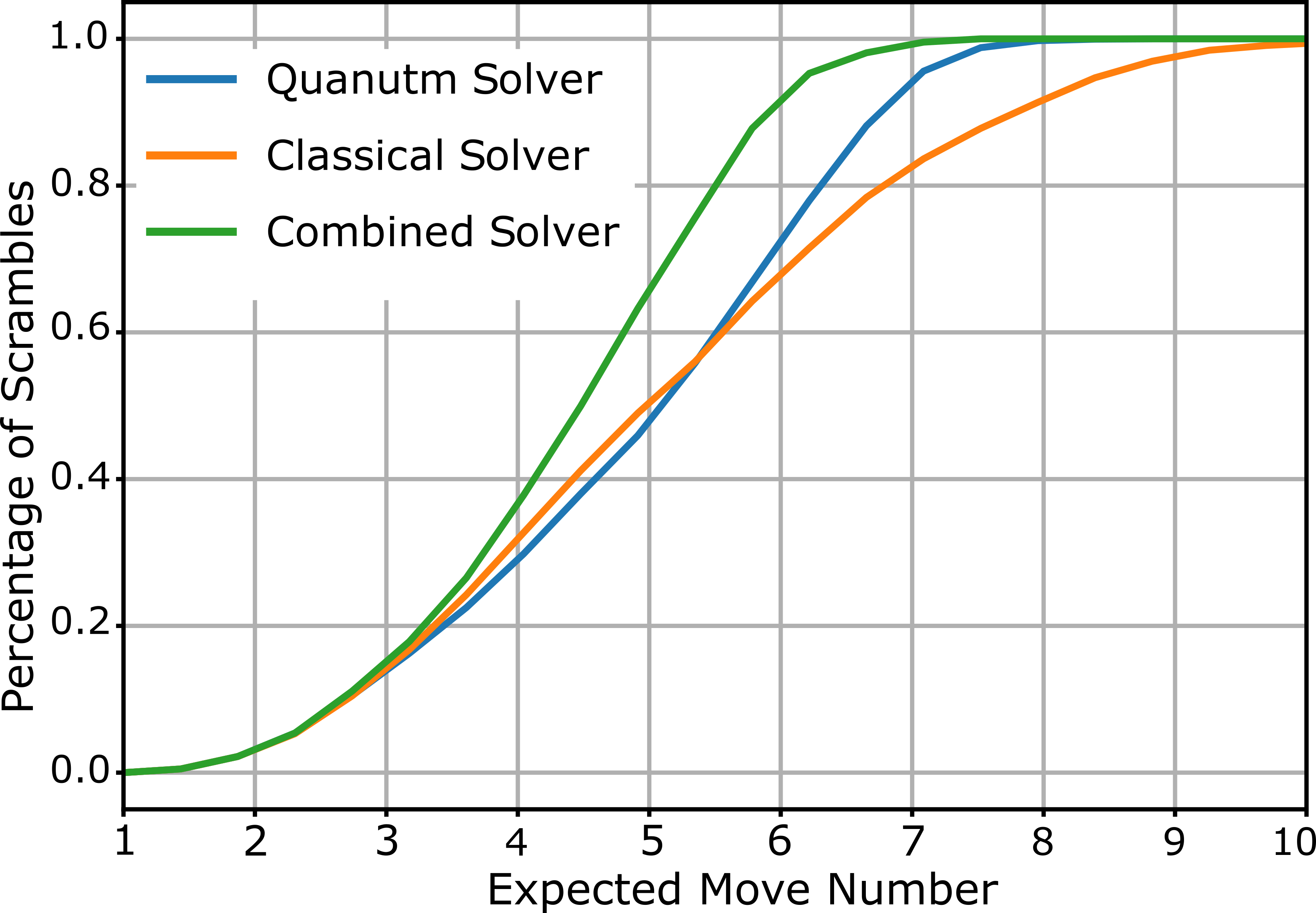
In Fig. 2 we simulate the performance of three solvers: the quantum solver with access to square root SWAPs, the classical solver with access to SWAPs, and a combined solver that can do both square root SWAPs and classical SWAPs each with just a single move. The classical solver can solve some scrambles much faster than the quantum solver, but the lack of versatility in the classical strategy leads to some scrambles taking many moves to solve. The combined solver mitigates this early advantage that comes from the faster SWAP action, but does not suffer from difficult scrambles. Overall, the classical solver does the worst on average with an average move count of 5.88 moves. The quantum solver is noticeably better taking only moves on average. And, as expected, the combined solver is much better at solving the puzzle in moves on average.
V Universality
Our puzzle corresponds to a six level qudit as explained in Section II. Although the state space of our puzzle is infinite, not every linear combination of basis states is achievable with just square root SWAPs starting from — ⟩. We now explore adding some additional actions to the solver’s repertoire so that all linear combinations become achievable. In quantum computing, a universal gate set enables one to generate an arbitrary approximation to any linear combination of basis states starting from any initial state. Specifically, if the set of operations generated by a gate set is dense in , then it is said to be a universal gate set for a -level qudit.
It might be helpful to first consider why the set of square root SWAPs is not universal. We determined this by applying the procedure introduced in [11], which checks two requirements. First, we check if the group generated from the set of square root SWAPs is infinite, which we previously mentioned is the case. Second, we find the set of matrices that commute with the adjoint representation of the generators. If this set is just scalar multiples of identity, then our puzzle is universal, but this is not the case.
To achieve universality, we can add additional gates to supplement the square root SWAPs. One simple additional gate is the gate
| (20) |
which applies a phase to one of the classical basis states, but does not permute any of the states amongst themselves. Although this gate does not have a clear interpretation in terms of solving the puzzle, as it is not related to an actual permutation of our puzzle pieces, it may still be related to the idea of piece parity in classical permutation puzzles. If we take the original gate set and include the gate, i.e. , and run the numerical proof, we find that this new gate set passes the universality test. The code is available here [13].
It is also possible to achieve universality by modifying the building blocks of our puzzle. If we allow different colored particles of our puzzle to also have different exchange statistics, e.g. green bosons and blue fermions. Now when a square root SWAPs exchanges the green bosons with each other and the blue fermions with each other they will pick up a different phase, similar to how we added this differential phase with . This phase difference, in addition to adding square root diagonal SWAPs or full diagonal SWAPs, is enough to make the gate set universal on this new puzzle. To verify this, we change the gate set that we input into the universality-checking algorithm so that this different phase is reflected. In fact this is equivalent to replacing one of the sets of fermions with empty sites. We show in Appendix C that these sites would have positive exchange statistics and are trivially indistinguishable, so they allow the puzzle to be universal.
VI Hilbert space dimension of larger board sizes
We have so far focused on the relatively small board that has unique classical board states which we mapped to a dimensional qudit Hilbert space. We now compute the qudit dimension of boards with more positions and colors. We will then briefly argue that the quantum advantage of the puzzle grows with board size.
One simple generalization of our puzzle is to consider two colors of particles in a larger grid of board positions. This will give us a total of arrangements of the board positions, of which many will be indistinguishable. For the simplest case where is even and thus we have particles of each color we can map this puzzle to an effective qudit dimension of
| (21) |
where we have divided through by the arangements of each color of indistinguishable particles. Interestingly, for even , the sequence of numbers given by is a well known integer sequence [14]. When is odd, we can simply assume that there is a single green fermion added, and then the asymptotic effective qudit dimension is identical to Eq. 21.
One can also consider boards, with colors of particles. In this case it does not matter if is odd or even, because each color of particle has indistinguishable configurations and we have colors. The equivalent qudit Hilbert space dimension grows as [15]
| (22) |
which grows much faster than Eq. 21.
For non-square puzzles it is useful to define a puzzle to be connected if for any two board positions there exist a series of nearest neighbor SWAPs that connect the two positions. Then we can consider a connected board with total board positions, that is populated with colors of particles with particle numbers such that . For such a board total number of board states or effective qudit Hilbert space dimension is
| (23) |
where the right-hand side is a multinomial coefficient. Clearly Eq. 21 and Eq. 22 are special cases of Eq. 23.
Let us briefly consider how the quantum advantage seen in Section IV might scale with board size. Providing an exact description is challenging, as it is known that finding the optimal solution to the classical puzzle is NP-hard [16]. Instead, we will provide a conjecture based on our observations in the puzzle.
We conjecture that the gap in performance between the classical and quantum solver will increase as board sizes become larger, favoring the quantum solver. This conjecture is based on the observation that the classical solver struggles to solve scrambles with less concentrated amplitudes, much more than the quantum solver does. As the size of the board increases, the number of classical basis states also increases greatly, so the proportion of scrambles with amplitude concentrated in a basis state should decrease. Because the quantum solver is able concentrated amplitude, it should suffer less from these “bad” scrambles.
VII A quantum cube puzzle
Previously, we have considered puzzles in two dimensions with nearest-neighbor SWAPs. This doesn’t capture the complexity of puzzles like the Rubik’s cube. Here, we introduce a quantum version of the Rubik cube shown in LABEL:fig:2x2x1_cube (a). The visible colored faces of the puzzle pieces are replaced with identical particles. We flatten the 3D puzzle into 2D, as depicted in LABEL:fig:2x2x1_cube(b), and consider permutations of the particles consistent with rotational configurations. In Appendix E, we briefly outline the full three-dimensional modeling of the puzzle. Surprisingly, in both cases the puzzle can be mapped onto the slide puzzle considered above.
The cube has six unique states, see Fig. 4, up to an orientation assumption. In this section, we assume that solving the cube depends only on the relative arrangement of colors, not the cube’s orientation.111This differs from our treatment of the slide puzzle in Section II. In 3D puzzles like the Rubik’s cube, the puzzle’s orientation is irrelevant, and ignoring this would unnecessarily expand the state space. Any scramble of this puzzle can be solved in at most three moves, i.e. “God’s number” is three.
The primitive moves on the puzzle are rotations of one of the portions of the puzzle. The possible moves on the cube are clockwise rotations of the Left, Right, Up, Down which are denoted [17], and the anti-clockwise versions are denoted with a prime, i.e. . In this puzzle the moves are sufficient to generate and solve all possible cube states, due to our orientation assumption. Specifically starting at the solved state the moves
| (24) |
generate the board states in Fig. 4.
It is possible to go through the same, albeit more complicated, procedure in the slide puzzle to correctly represent the underlying identical particles as we did in Appendix A, see Appendix E. As the flattened board state is too unwieldy to fit inside a ket, we will instead prescribe a canonical ordering of the states with the following kets
| (25) |
In Fig. 4, we give the mapping between these kets and the cube state.
[width=0.25]b0
\includestandalone[width=0.25]b1
\includestandalone[width=0.25]b2
\includestandalone[width=0.25]b3
\includestandalone[width=0.25]b4
\includestandalone[width=0.25]b5
In the flattened form, it is difficult to see how the rotations change the state, as the natural moves are no longer a SWAP of two identical particles. The rotations effectively swap several particles. For this reason, it is useful to think of the moves as permutations. Thus transitioning between board states is a permutation of several particles so we denote the permutations as
| (26) |
which are self inverse so and . Acting these permutations on the board indeed transitions the board to a new state, e.g. and . In Appendix D, we give the matrix representation of the permutation matrices. This simply reproduces the classical puzzle behaviour and because this is a six dimensional Hilbert space it is equivalent to the 2D slide puzzle.
As before, we choose to add a new action that a solver can take, the square root of a permutation
| (27) |
where . Acting on the solved state produces a superposition as you would expect e.g.
| (28a) | ||||
| (28b) | ||||
As before, sequences of noncommutting square root permutations lead to states that are no longer equal superpositions. And thus we have created a quantum version of the Rubik’s cube with a state space that is analogous to our slide puzzle.
In Appendix E, we give a treatment of the puzzle in 3D using rotations. Ultimately we arrive back to a puzzle with six unique states and add a square root SWAP to make the puzzle more quantum.
VIII Conclusion
We have introduced a quantum generalization of permutation puzzles which does not have a simple classical analogue. The core idea was to represent the different colored pieces of a permutation puzzle with sets of identical quantum particles and use a quantum move that created superpositions between classically allowed states. This puzzle can be solved deterministically with quantum moves or, with the addition of measurements, be solved nondeterministically with just classical moves.
With superpositions, the number of unique allowed states of the puzzle is infinite, unlike common permutation puzzles from toy stores. While this bigger state space allows for a richer puzzle structure we can also consider making finite quantum puzzles. One way to do this would be, for the case of e.g. identical fermions, to consider the allowed moves to be a subset of fermionic Gaussian unitaries [18, 19, 20] that correspond to discrete Clifford elements [21]. Such a restriction would result in a discrete (but large) state space. Since the state space and set of actions are both finite, these versions of the puzzles could be mapped onto classical permutation puzzles, albeit ones with very strange geometries.
There are several questions that we think naturally arise from our discussion here. First, there is the question of implementation. Arrays of ultracold atoms in optical lattices [22, 23, 24] might be a natural platform because confinement and swapping of both fermionic and bosonic atoms has been demonstrated. Moreover recent experiments have demonstrated confinement of multiple species of atoms [25, 26, 27]. Quantum dot plaquettes [28] could make an appealing experimental platform given recent experimental demonstrations [29].
The second question we highlight is: what is the “puzzle group” generated by the square root SWAPs? The group is not as our actions are not universal for . The actions may be universal on for some .
Finally, there are many more permutation puzzles (classical and quantum) than we have described here. On the quantum side one could imagine replacing the fermions and bosons with Anyons [30]. On the classical side we think our examples above provide a recipe to quantize permutation puzzles:
-
1.
Replace the structure of the puzzle with sets of identical particles. If the quantum particles are appropriately indistinguishable then the state space of the particles will match the state space of the classical puzzle.
-
2.
The classical primitive moves (swaps, permutations, rotations) can easily be quantized as permutation matrices acting on the state space. These permutation matrices are unitary and naturally act on the Hilbert space of the quantum puzzle.
-
3.
To achieve a non-classical puzzle one adds a quantum move. We have argued that unitaries that are generated by the exponential of permutations are a natural candidate.
Acknowledgments: The authors acknowledge helpful discussions with Todd Brun, Shawn Geller, Joshua Grochow, Kyle Gulshen, and Robert Smith. NL, AK, and JC were supported by the University of Colorado Boulder. MTG would like to thank Sharon Anderson and the CU Boulder Summer Program for Undergraduate Research (CU SPUR) for their support.
References
- Mulholland [2021] J. Mulholland, Permutation puzzles: a mathematical perspective, Departement Of mathematics Simon fraser University (2021).
- Zhao et al. [2022] J. Zhao, T. Zhang, J. Jiang, T. Fang, and H. Ma, Color image encryption scheme based on alternate quantum walk and controlled rubik’s cube, Scientific Reports 12, 14253 (2022).
- Thomson and Eisert [2024] S. J. Thomson and J. Eisert, Unravelling quantum dynamics using flow equations, Nature Physics 10.1038/s41567-024-02549-2 (2024).
- Bao and Hartnett [2024] N. Bao and G. S. Hartnett, Twisty-puzzle-inspired approach to clifford synthesis, Phys. Rev. A 109, 032409 (2024).
- Wang and Bo [2024] Y. Wang and M. Bo, Understanding energy level structure using quantum rubik’s cube (2024), arXiv:2403.01195 [quant-ph] .
- Shi et al. [2020] F. Shi, M. Hu, L. Chen, and X. Zhang, Strong quantum nonlocality with entanglement, Phys. Rev. A 102, 042202 (2020).
- Corli et al. [2023] S. Corli, L. Moro, D. E. Galli, and E. Prati, Casting rubik’s group into a unitary representation for reinforcement learning, Journal of Physics: Conference Series 2533, 012006 (2023).
- Bobrow et al. [2018] E. Bobrow, K. Stubis, and Y. Li, Exact results on itinerant ferromagnetism and the 15-puzzle problem, Phys. Rev. B 98, 180101 (2018).
- Pauli [1940] W. Pauli, The connection between spin and statistics, Phys. Rev. 58, 716 (1940).
- Spivak et al. [2022] D. Spivak, M. Y. Niu, B. C. Sanders, and H. de Guise, Generalized interference of fermions and bosons, Phys. Rev. Res. 4, 023013 (2022).
- Sawicki and Karnas [2017a] A. Sawicki and K. Karnas, Criteria for universality of quantum gates, Phys. Rev. A 95, 062303 (2017a).
- Sawicki and Karnas [2017b] A. Sawicki and K. Karnas, Universality of Single-Qudit Gates, Annales Henri Poincaré 18, 3515 (2017b).
- Lordi et al. [2024] N. Lordi, A. Kyle, M. Trank-Greene, and J. Combes, Quantum permutation puzzles codebase (2024).
- Royappa [2003] A. T. Royappa, Sequence A081623 in the On-line Encyclopedia of Integer Sequences (n.d.), https://oeis.org/A081623 (2003), accessed on May 20 2024.
- Friedman [2001] E. Friedman, Sequence A034841 in the On-line Encyclopedia of Integer Sequences (n.d.), https://oeis.org/A034841 (2001), accessed on May 20 2024.
- Ratner and Warmuth [1986] D. Ratner and M. Warmuth, Finding a shortest solution for the nxn extension of the 15-puzzle is intractable, in Proceedings of the Fifth AAAI National Conference on Artificial Intelligence, AAAI’86 (AAAI Press, 1986) p. 168–172.
- Singmaster [1981] D. B. Singmaster, Notes on Rubik’s Magic Cube (Penguin Books., 1981) https://www.amazon.com/exec/obidos/ASIN/0894900439/.
- Knill [2001] E. Knill, Fermionic linear optics and matchgates (2001), arXiv:quant-ph/0108033 [quant-ph] .
- Bravyi and Kitaev [2002] S. B. Bravyi and A. Y. Kitaev, Fermionic quantum computation, Annals of Physics 298, 210 (2002).
- Jozsa and Miyake [2008] R. Jozsa and A. Miyake, Matchgates and classical simulation of quantum circuits, Proceedings of the Royal Society A: Mathematical, Physical and Engineering Sciences 464, 3089 (2008).
- Zhao et al. [2021] A. Zhao, N. C. Rubin, and A. Miyake, Fermionic partial tomography via classical shadows, Phys. Rev. Lett. 127, 110504 (2021).
- Endres et al. [2016] M. Endres, H. Bernien, A. Keesling, H. Levine, E. R. Anschuetz, A. Krajenbrink, C. Senko, V. Vuletic, M. Greiner, and M. D. Lukin, Atom-by-atom assembly of defect-free one-dimensional cold atom arrays, Science 354, 1024 (2016).
- Ebadi et al. [2021] S. Ebadi, T. T. Wang, H. Levine, A. Keesling, G. Semeghini, A. Omran, D. Bluvstein, R. Samajdar, H. Pichler, W. W. Ho, S. Choi, S. Sachdev, M. Greiner, V. Vuletić, and M. D. Lukin, Quantum phases of matter on a 256-atom programmable quantum simulator, Nature 595, 227 (2021).
- Kaufman and Ni [2021] A. M. Kaufman and K.-K. Ni, Quantum science with optical tweezer arrays of ultracold atoms and molecules, Nature Physics 17, 1324 (2021).
- Singh et al. [2022] K. Singh, S. Anand, A. Pocklington, J. T. Kemp, and H. Bernien, Dual-element, two-dimensional atom array with continuous-mode operation, Phys. Rev. X 12, 011040 (2022).
- Anand et al. [2024] S. Anand, C. E. Bradley, R. White, V. Ramesh, K. Singh, and H. Bernien, A dual-species rydberg array, Nature Physics 10.1038/s41567-024-02638-2 (2024).
- Beterov and Saffman [2015] I. I. Beterov and M. Saffman, Rydberg blockade, förster resonances, and quantum state measurements with different atomic species, Phys. Rev. A 92, 042710 (2015).
- Buterakos and Das Sarma [2019] D. Buterakos and S. Das Sarma, Ferromagnetism in quantum dot plaquettes, Phys. Rev. B 100, 224421 (2019).
- Dehollain et al. [2020] J. P. Dehollain, U. Mukhopadhyay, V. P. Michal, Y. Wang, B. Wunsch, C. Reichl, W. Wegscheider, M. S. Rudner, E. Demler, and L. M. K. Vandersypen, Nagaoka ferromagnetism observed in a quantum dot plaquette, Nature 579, 528 (2020).
- Wilczek [1982] F. Wilczek, Quantum mechanics of fractional-spin particles, Phys. Rev. Lett. 49, 957 (1982).
Appendix A Inner product in explicit Fermion representation
The permutation puzzle has four physical locations:
| (29) |
To formalize our diagrammatic representation, we want to represent these locations (or positions) with a tensor product structure as
| (30) |
Any of these locations can hold a green or a blue fermion e.g. would decompose further as
| (31) |
Thus one can even write down fermionic creation operators to transition from the vacuum to a particular state. In the main text we represented the solved state as
| (32) |
Let’s rewrite this state with respect to the tensor product structure in Eq. 30 and leave the color tensor product in Eq. 31 implicit:
| (33) |
this gives meaning to the diagrammatic representation in Eq. 32. As another example lets consider another the board state
| (34) |
We can compute the inner product between these term by term. However it is easy to compute one term explicitly
| (35) |
where we separated the tensor product by locations, and the commas separate color. We can do this for all such terms in Eq. 33 and Eq. 34 to show that
which is Eq. 10.
Appendix B slide puzzle Qudit mapping
In the main text, see Eq. 6, we defined board states where the underlying identical particles were (anti) symmetrized
By performing the SWAP operations we can list all possible board states
Then by computing inner products of the underlying identical particle one can show that the six states are orthogonal. Thus these states correspond to a 6 dimensional qudit which we represent by the following column vectors
| (36a) | ||||
| (36b) | ||||
| (36c) | ||||
| (36d) | ||||
| (36e) | ||||
| (36f) | ||||
For the moment let’s focus on the fermionic case. To determine the 6 dimensional unitaries that correspond to the SWAP operations we simply act a particular SWAP on the basis of board states. This will represent the unitary in the board basis. For example, consider the Up SWAP operation acting on the solved board state
| (37) |
This indicates that the unitary has a in the top left position. Acting the Up SWAP on the remaining board states gives
| (38a) | ||||
| (38b) | ||||
| (38c) | ||||
| (38d) | ||||
| (38e) | ||||
If we collect all of this information together in a matrix we find the Unitary matrix that corresponds to applying a Up SWAP is
| (39) |
which is a signed permutation matrix.
If we repeat this process for the remaining SWAP operations we find
| (40) |
and
| (41) |
and
| (42) |
The bosonic case is similar except there are no minus signs in the Unitaries so they are simply permutation matrices.
Appendix C Fermionic vs Bosonic SWAPs
Lets imagine a the simplest case where we would have a swap of identical particles. We consider 2 sites each with at most 1 particle. For now consider only one species. We can write down distinguishable state as
| (43) |
where the first indecies account for particle location and the numbers indicate the number of paricles in that location, i.e means no particle in the first location and one particle in the second location.
For bosons the Full swap matrix acting on this Hilbert space is a permutation matrix with explicit form,
| (44) |
which acts on the states as follows
| (45) | ||||
The only difference with fermions is in the last element
| (46) |
This shows that swapping two instances of fermionic vacuum does not pick up a phase, i.e . Additionally swapping fermions with vacuum picks up no phase, but swapping two identical fermions picks up a minus sign.
Now if we go back to our 2x2 puzzle with two green particles and two blue particles we will quickly rederive the swapping relations. First we must note that swapping a green and blue fermions is really an emergent action. This action is a result of swapping a green particle in location 1 with green vacuum in location 2 and a blue particle in location 2 with blue vacuum in location 1. Each swap of particle and vacuum with pick up no phase since for both bosons and fermions .
So for both fermions and bosons it is true that
| (47a) | ||||
| (47b) | ||||
| (47c) | ||||
| (47d) | ||||
But they differ when identical particles are exchanged, e.g for bosons
| (48a) | ||||
| (48b) | ||||
and for fermions
| (49a) | ||||
| (49b) | ||||
Now a final question is what happens in the situation where we have green fermions and blue bosons. It is easy to show that all the situations in which no identical particles are swapped results in no phase since this is true for both bosons and fermions. Now for a specific swap we just need to determine which particles are swapped. For example if we swap the top particles of we would be swapping green particles which are fermions so . But if we apply the same swap to we would swap the blue particles which are bosons so no phase would be introduced.
Similarly if we remove the bosons and are left with two empty sites of fermionic vacuum we would have the same behavior. This follows directly from our previous note that fermionic vacuum can be exchanged without picking up a phase.
Appendix D Cube Qudit mapping
As before we map the six cube states to a 6 dimensional qudit. The board states are represented by the following column vectors
To determine the matrix elements of we the action on the cube and map its actions on the basis states and find
| (50) | ||||
It’s similarly straightforward to show that
| (51) | ||||
From these relations we define the permutation matrix (assuming bosonic statistics)
| (52) |
in this case the inverse . The permutation matrix for the action is
| (53) |
Appendix E The 3D Treatment of the cube
Our goal is to show that rotating a collection of particles simply permutes the board states and thus justifies the permutation treatment given in the main text. For simplicity we will consider the particles in this section to be Bosons.
Let’s start by defining the location of the quantum particles in 3D by the position vector. Because we will need to specify 16 locations we introduce a subscript e.g. a particle at location 1 is at the position
| (54) |
these locations are fixed and don’t depend on the color of the particle, see Fig. 5.
\includestandalone[width=0.2]axis \includestandalone[width=0.33]cube_2x2x1_labels \includestandalone[width=0.27]b_lab
We limit rotations to along any axis to prevent changing the puzzle’s shape, keeping it within the six board configurations. Now we want to determine how a rotation, e.g. rotation about the -axis acts on the collection of particles. Recall that the angular momentum operator, in this case
| (55) |
is the generator of rotations in the space of physical states. The corresponding rotation operator is , which can be written in terms of its SO(3) action
| (56) |
so that
| (57) |
where is the position wavefunction of the ’th particle.
However our moves are not simply a rotation about the axis. The move for example, is a rotation about the axis restricted to any positive coordinate, i.e. , so that the cubes below don’t move. We denote these restricted rotations as
| (58) |
and the related rotation about the positive axis would be .
Now consider the quantum state of the bosons. To be explicit we consider point like bosons denote the wavefunction of a single particle at location is denoted by . So if the third yellow particle was at location
| (59) |
where . To simplify the description of indistinguishable particles we will denote the wavefunction of four e.g. yellow particles at four locations
| (60) |
Using this notation we can denote the (anti) symmetrized wavefunction as
| (61) | ||||
The solved state wavefunction will be denoted as
| (62) | ||||
while for the first state it would be
| (63) | ||||
and similarly for the ’th board state.
Defining the correctly (anti) symmetrized wavefunction for the 16 particles and showing that it transforms correctly is tedious, so we present those calculations in Section E.1 for the following case
| (64) |
With some more work, one can show that
| (65) | ||||
which is consistent with the classical moves Eq. 24 and the permutation description. That means we have a fully quantum description, in 3D, of our puzzle.
In order to add an analogous move to the square root SWAP we need to be able to implement the operation
| (66) |
Physically implementing such a rotation in 3D seems hard. One possible way is to do a controlled rotation gate, controlled of e.g. a qubit in the plus state, and measure in the qubit basis. Then conditional on getting the outcome the square root SWAP operation would be enacted.
E.1 ‘U’ move on the solved state
In this subsection we show explicitly that
E.1.1 Red and Orange particles
From looking at Fig. 5 we see that the wavefunction of the red particles in the solved state is
| (67) |
We can see in Fig. 4 that the red particles remain in the same location after the rotation so lets check that. Assume that
| (68) |
then using Eq. 57 we can show
| (69) |
which just means that there is no change, as expected. The orange particles are completely unaffected by this rotation, so we don’t consider them.
E.1.2 Green and Blue particles
For the green and blue particles, we define locations
| (70) | ||||
The wavefunctions before the rotation are
| (71) | ||||
and after
| (72) | ||||
which is consistent with the board state.
E.1.3 White and Yellow particles
Initally the yellow particles are at the locations
| (73) | ||||
and the white particles are at
| (74) | ||||
The wave function of the yellow particles in the solved state is
| (75) | ||||
as only acts on locations 3 and 4 we only expect those particles to transform and similarly for the white particles. After acting the rotation we find
| (76) | ||||
In summary, what we have shown is that
| (77) |