Capturing the Elusive Curve-Crossing in Low-Lying States of Butadiene With Dressed TDDFT

Abstract

A striking example of the need to accurately capture states of double-excitation character in molecules is seen in predicting photo-induced dynamics in small polyenes. Due to the coupling of electronic and nuclear motions,the dark 2¹Ag state, known to have double-excitation character, can be reached after an initial photo-excitation to the bright ¹Bu state via crossings of their potential energy surfaces. However, the shapes of the surfaces are so poorly captured by most electronic structure methods, that the crossing is missed or substantially mis-located. We demonstrate that the frequency-dependent kernel of dressed TDDFT beyond Tamm-Dancoff successfully captures the curve-crossing, providing an energy surface close to the highly accurate but more expensive $\delta$-CR-EOMCC(2,3) benchmark reference. This, along with its accurate prediction of the excitation character of the state makes dressed TDDFT a practical and accurate route to electronic structure quantities needed in modeling ultrafast dynamics in molecules.

I Introduction

Linear polyenes have long been the focus of intensive experimental and theoretical work owing to their importance in biological and technologically important systems Hudson and Kohler (1972); Schulten and Karplus (1972); Schulten et al. (1976); Andrews and Hudson (1978); Cave and Davidson (1987); Orlandi et al. (1991); Fuss et al. (1998); Christensen et al. (2004); Levine and Martínez (2007); Levine and MartÃnez (2009); Komainda et al. (2013); Barford (2022). In particular the photophysical behavior of the smallest polyenes, s-trans-butadiene and s-trans-hexatriene, is of significant interest in organic electronics and photovoltaics Papagiannakis et al. (2002), and are viewed as representative motifs of polyenes responsible for triggering vision Orlandi et al. (1991). Despite this longstanding interest, accurately describing the electronic structure and photodynamics of linear polyenes has proven challenging for theoretical methods, leading to unreliable predictions of relaxation processes through conical intersections after photo-excitation. These difficulties stem from the nature of the low-lying excited states in these molecules, particularly the dark 2¹Ag state, due to its partial doubly-excited character Ohmine et al. (1978); Lappe and Cave (2000), which many single reference methods struggle to capture. Conventional computational techniques such as complete active space self-consistent field (CASSCF) and equation of motion coupled cluster with singles and doubles (EOM-CCSD) frequently fall short in describing these excited states Loos et al. (2019); Park et al. (2021). Even though these approximate methods can be adjusted to describe a single-point calculation of 2¹Ag accurately, their reliability across geometry variations is suspect. They typically incorrectly predict the crossing of the potential energy surfaces of the two lowest excited states, 1¹Bu and 2¹Ag Park et al. (2021). As a result, many studies have struggled to describe the ultrafast dynamics of polyenes with the precision required for predicting observed results.

While it is known that the challenge essentially lies in incorporating double excitations in the descriptions of the excited states, most computational techniques that do accurately handle these states tend to become very expensive for longer polyenes. For instance, the $\delta$-CR-EOMCC(2,3) approach of Refs.Fradelos et al. (2011); Piecuch et al. (2015), which corrects the excited-state potentials obtained with EOMCCSD for the effects of triple excitations, correctly captures the curve crossing in s-trans-butadiene and s-trans-hexatriene Park et al. (2021). However, developing a method that achieves comparable accuracy at a lower computational cost would significantly benefit calculations for larger systems.

In principle, time-dependent density functional theory (TDDFT) Runge and Gross (1984); Casida (1995); Petersilka et al. (1996) could serve as a low-cost alternative due to its famously tolerable scaling. However, in practice the adiabatic approximation inherent in its standard linear response formulation ignores double excitation contributions, and as a result it struggles to accurately describe the energy ordering and shapes of the surfaces for these states Park et al. (2021). Going beyond adiabatic TDDFT (ATDDFT), so-called dressed TDDFT approaches have been developed Tozer et al. (1999); Tozer and Handy (2000); Cave et al. (2004); Casida (2005); Mazur and Włodarczyk (2009); Mazur et al. (2011); Romaniello et al. (2009); Sangalli et al. (2011); Huix-Rotllant et al. (2011); Casida and Huix-Rotllant (2012, 2016); Maitra (2022); Dar and Maitra (2023), in which a frequency-dependent kernel is designed to incorporate contributions from double excitations. The original version operated within the Tamm-Dancoff approximation Maitra et al. (2004); Cave et al. (2004); Casida (2005); Mazur and Włodarczyk (2009); Casida and Huix-Rotllant (2016), denoted here as dressed Tamm-Dancoff (DTDA), and has successfully predicted the energies of double excitations across a variety of molecules Cave et al. (2004); Huix-Rotllant et al. (2011); Mazur and Włodarczyk (2009); Mazur et al. (2011); Maitra (2022). However, because the Tamm-Dancoff approximation inherently does not preserve oscillator strengths, DTDA cannot be used reliably for transition properties including the non-adiabatic couplings between states needed for dynamics. In Ref. Dar and Maitra (2023), we derived a frequency-dependent kernel designed to function within the full TDDFT linear response framework, ensuring that the oscillator strength sum rule is preserved. Its performance on model as well as real systems, including the lowest ${}^{1}D$ excitations of the Be atom and LiH molecule across varying interatomic distances was found to be satisfactory. This kernel redistributes the transition density of a Kohn-Sham (KS) single excitation into a mix of single and double excitations, resulting in better predictions for transitions between excited states, as demonstrated in Ref. Dar and Maitra (2023). The examples in Ref. Dar and Maitra (2023) involved cases where one single excitation couples with a double excitation while more commonly, and in the case of the $2^{1}$Ag state of linear polyenes, the state is composed of several single-excitations mixing with a double-excitation with respect to the ground-state KS reference. Here we extend the approach of Ref Dar and Maitra (2023) to scenarios where multiple single excitations couple with a double excitation. We show that the potential energy surfaces of 1¹Bu and 2¹Ag for s-trans-butadiene resulting from our dressed TDDFT (DTDDFT) display a crossing close to that predicted by the highly-accurate $\delta$-CR-EOMCC(2,3) Piecuch et al. (2015); Park et al. (2021) method, which we use as a benchmark in this study.

II Theory

The fundamental of idea of DTDDFT beyond DTDA was presented in Ref. Dar and Maitra (2023), motivated by needing accurate oscillator strengths and transition densities, in addition to the energies. The equations were derived there for the case when the state of interest involves one single excitation out of the KS ground-state reference mixing with one double excitation. One begins with the time-independent Schrodinger equation in the following form:

$$(H-E_{0})^{2}\Psi=\omega^{2}\Psi$$ (1)

where $E_{0}$ is the ground state energy and $\omega$ represents the excitation frequency. In the truncated Hilbert space of the doubly-excited determinant $|D\rangle$ and singly-excited determinant $|Q\rangle$, diagonalization of the operator $(H-E_{0})^{2}$ leads to

$$\omega^{2} = (H_{QQ}-E_{0})^{2}+|H_{QD}|^{2}$$ (2)

$$\times \Bigg{[}1+\frac{(H_{QQ}+H_{DD}-2E_{0})^{2}}{\omega^{2}-\left[(H_{DD}-E_{0})^{2}+|H_{QD}|^{2}\right]}\Bigg{]}$$

where $H_{AB}$ are the matrix elements of the true Hamiltonian between KS states. Obtaining excitation energies in TDDFT however does not proceed through diagonalization, but instead through a linear response procedure, where the KS single excitations get corrected to the exact ones via the exchange-correlation (xc) kernel $f_{\scriptscriptstyle\rm XC}({\bf r},{\bf r}^{\prime},\omega)$ Casida (1995); Petersilka et al. (1996). Ref. Dar and Maitra (2023) mapped Eq. (2) on to the TDDFT linear response equation truncated to one single excitation, and thereby extracted a frequency-dependent xc kernel. The first term in Eq. 2, which is the contribution to $\omega^{2}$ from the single excitation, was replaced with the ATDDFT small matrix approximation (SMA) value, while the residual part, with $E_{0}$ replaced by $H_{00}$ to balance the errors in accordance with what was done in Ref. Maitra et al. (2004), was interpreted as a frequency-dependent kernel in a dressed SMA (DSMA):

$$f_{{\scriptscriptstyle\rm XC}\,QQ}^{\rm DSMA_{0}}(\omega) = f_{{\scriptscriptstyle\rm XC}\,QQ}^{\rm adia}+\frac{|H_{QD}|^{2}}{4\nu_{q}}$$

$$\times \left(1+\frac{(H_{QQ}+H_{DD}-2H_{00})^{2}}{\left[\omega^{2}-\left((H_{DD}-H_{00})^{2}+H_{QD}^{2}\right)\right]}\right)\,.$$

Here $f_{{\scriptscriptstyle\rm XC}\,QQ}^{\rm adia}$ denotes the diagonal matrix element of an adiabatic xc-kernel, whose general expression is

$$\small f^{\rm adia}_{{\scriptscriptstyle\rm XC}\,QQ^{\prime}}(\omega)=\int d^{3}r\int d^{3}r^{\prime}\,\Phi_{Q}^{*}(\mathbf{r})\,f^{\rm adia}_{\scriptscriptstyle\rm XC}(\mathbf{r},\mathbf{r}^{\prime},\omega)\,\Phi_{Q^{\prime}}(\mathbf{r^{\prime}})$$ (4)

in which $\Phi_{Q}^{*}(\mathbf{r})=\phi_{i}({\bf r})\phi_{a}({\bf r})$ is the product of orbitals involved in the KS single excitation $Q:i\rightarrow a$. Eq. (II) represents a dressed SMA (DSMA), and this kernel should be used within the SMA. Further, two variants of Eq. (II) were proposed by making the following replacements

$$(H_{QQ}+H_{DD}-2H_{00})^{2} \xrightarrow{\rm{DSMA}_{\scriptscriptstyle\rm S}} (\nu_{Q}+\nu_{D})^{2}$$

$$(H_{DD}-H_{00})^{2} \xrightarrow{\hskip 28.45274pt} \nu_{D}^{2}$$ (5)

and

$$(H_{QQ}+H_{DD}-2H_{00})^{2} \xrightarrow{\rm{DSMA}_{\displaystyle\rm a}} (\Omega_{Q}^{A}+\Omega_{s1}^{A}+\Omega_{s2}^{A})^{2}$$

$$(H_{DD}-H_{00})^{2} \xrightarrow{\hskip 28.45274pt} (\Omega_{s1}^{A}+\Omega_{s2}^{A})^{2}$$ (6)

where $\nu_{Q}$ and $\nu_{D}\equiv\nu_{s1}+\nu_{s2}$ are the KS frequencies of the single and double excitations, obtained from KS orbital energy differences (e.g. $\nu_{Q}=\epsilon_{a}-\epsilon_{i}$) and $\Omega_{Q(s1,s2)}^{A}$ are the ATDDFT-corrected frequencies of the single excitation $Q$ and the two single excitations $s_{1},s_{2}$ that compose the KS double-excitation. These two variants are much easier than DSMA₀ to implement computationally as they require fewer two-electron matrix elements to be computed: Apart from $H_{QD}$ one can extract all the other quantities directly from the ATDDFT calculation.

To extend this approach to cases where more than one single excitation couples with a double excitation, we follow a similar strategy as above but explicitly mix in more than one single KS excitation by first expressing the single-excitation component $|Q\rangle$ of the interacting state as a linear combination of all the KS single excitations $|q\rangle$

$$|Q\rangle=\displaystyle\sum_{q}c_{q}|q\rangle.$$ (7)

Diagonalization in the space of all these single excitations plus the double excitation that couples with them again leads to Eq. 2 with the following redefinitions

$$H_{QQ}=\sum_{q,q^{\prime}}c_{q}^{*}c_{q^{\prime}}H_{qq^{\prime}}$$ (8)

and

$$H_{QD}=\sum_{q}c_{q}^{*}H_{qD}\,.$$ (9)

Using these forms, Eq. (2) becomes

$$\omega^{2}=\left(\sum_{q,q^{\prime}}c_{q}^{*}c_{q^{\prime}}H_{qq^{\prime}}-H_{00})\right)^{2}+\sum_{q,q^{\prime}}c_{q}^{*}c_{q^{\prime}}H_{qD}H_{Dq^{\prime}}$$

$$\times\left[1+\frac{(\sum_{q,q^{\prime}}c_{q}^{*}c_{q}^{\prime}H_{qq^{\prime}}+H_{DD}-2H_{00})^{2}}{\omega^{2}-\left[(H_{DD}-H_{00})^{2}+\sum_{q,q^{\prime}}c_{q}^{*}c_{q^{\prime}}H_{qD}H_{Dq^{\prime}}\right]}\right].$$ (10)

As in the case of a single single-excitation coupling to a double, this result of diagonalization is used to inspire an approximation for a frequency-dependent TDDFT xc kernel for the present case of several single-excitations coupling to a double. This time, we are beyond the SMA, and consider the full TDDFT matrix,

$$\Omega(\omega)_{qq^{\prime}}=\nu^{2}_{q}\delta_{qq^{\prime}}+4\sqrt{\nu_{q}\nu_{q^{\prime}}}f_{{\scriptscriptstyle\rm HXC}\,qq^{\prime}}(\omega)\,$$ (11)

whose eigenvalues give the (in-principle exact) squares of the frequencies $\omega^{2}$ of the true system. Here $\nu_{q}$ is the frequency of the KS single excitation $|q\rangle$ and $f_{{\scriptscriptstyle\rm HXC}\,qq^{\prime}}(\omega)$ is matrix element (Eq. (4)) of the Hartree-xc kernel

$$f_{\scriptscriptstyle\rm HXC}(\mathbf{r},\mathbf{r}^{\prime},\omega)=\frac{1}{|\mathbf{r}-\mathbf{r}^{\prime}|}+f_{\scriptscriptstyle\rm XC}(\mathbf{r},\mathbf{r}^{\prime},\omega)\,.$$ (12)

Now, to construct the approximation to the xc kernel, we first require that in the limit of all the couplings between the single and double excitations in Eq. (10) going to zero, $H_{qD}\rightarrow 0$, the procedure reduces to Eq. (11) with an adiabatic approximation to the kernel. The justification is that ATDDFT is typically accurate for states of single-excitation character, provided the ground-state approximation used has appropriate long-ranged characters when needed Stein et al. (2009); Maitra (2016, 2017); Kümmel (2017). That is, we replace the diagonalization amongst the KS singles in Eq. (10) with the adiabatic part of Eq. (11) i.e.

$$\left(\sum_{q,q^{\prime}}c_{q}^{*}c_{q^{\prime}}H_{qq^{\prime}}-H_{00})\right)^{2}\Rightarrow\nu^{2}_{q}\delta_{qq^{\prime}}+4\sqrt{\nu_{q}\nu_{q^{\prime}}}f^{\rm{adia}}_{{\scriptscriptstyle\rm HXC}\,qq^{\prime}}\,$$ (13)

This then suggests the following approximation for the frequency-dependent DTDDFT xc kernel matrix:

$$f^{\mathrm{DTDDFT_{0}}}_{{\scriptscriptstyle\rm XC}\,qq^{\prime}}(\omega) = f^{\rm{adia}}_{{\scriptscriptstyle\rm XC}\,qq^{\prime}}+X^{0}_{qq^{\prime}}(\omega)$$ (14)

where

$$X^{0}_{qq^{\prime}}(\omega)=\frac{H_{qD}H_{Dq^{\prime}}}{4\sqrt{\nu_{q}\nu_{q^{\prime}}}}\left[1+\frac{(H_{qq^{\prime}}+H_{DD}-2H_{00})^{2}}{\omega^{2}-(H_{DD}-H_{00})^{2}}\right]$$ (15)

We dropped the last term in the denominator of Eq. (10) for the following two reasons. First, it would give the kernel an unphysical dependence on the arbitrary sign choice for the states $q,q^{\prime}$. Second, taking the Tamm-Dancoff limit of our approximation, where “backward” transitions are neglected, it should reduce to the previously-derived DTDA of Refs. Cave et al. (2004); Mazur and Włodarczyk (2009), but this only happens if this term is dropped (see the Supporting Information).

Eq. (14), together with two variants that reduce the computational cost, analogous to Eqs. (5)–(6),

$$f_{{\scriptscriptstyle\rm HXC}\,qq^{\prime}}^{\mathrm{DTDDFT_{\scriptscriptstyle\rm S}}}(\omega)=f^{\rm{adia}}_{{\scriptscriptstyle\rm HXC}\,qq^{\prime}}+X^{{}_{\scriptscriptstyle\rm S}}_{qq^{\prime}}(\omega)$$ (16)

$$f_{{\scriptscriptstyle\rm HXC}\,qq^{\prime}}^{\mathrm{DTDDFT_{\displaystyle\rm a}}}(\omega)=f^{\rm{adia}}_{{\scriptscriptstyle\rm HXC}\,qq^{\prime}}+X^{{}_{\displaystyle\rm a}}_{qq^{\prime}}(\omega)$$ (17)

where

$$X^{{}_{\scriptscriptstyle\rm S}}_{qq^{\prime}}(\omega)=\frac{H_{qD}H_{Dq^{\prime}}}{4\sqrt{\nu_{q}\nu_{q^{\prime}}}}\left[1+\frac{(\nu_{q}+\nu_{D})(\nu_{q^{\prime}}+\nu_{D})}{\omega^{2}-\nu_{D}^{2}}\right]$$ (18)

and

$$X^{{}_{\displaystyle\rm a}}_{qq^{\prime}}(\omega)=\frac{H_{qD}H_{Dq^{\prime}}}{4\sqrt{\nu_{q}\nu_{q^{\prime}}}}\left[1+\frac{(\Omega_{q}^{A}+\Omega_{s1}^{A}+\Omega_{s2}^{A})(\Omega_{q^{\prime}}^{A}+\Omega_{s1}^{A}+\Omega_{s2}^{A})}{\omega^{2}-(\Omega_{s1}^{A}+\Omega_{s2}^{A})^{2}}\right]$$ (19)

form the central equations of this paper. They define three non-adiabatic kernel approximations that account for a double-excitation mixing with multiple single excitations. On the one hand, these equations extend the DSMA approximations of Ref. Dar and Maitra (2023) to the case where the state of double-excitation character involves several KS single excitations instead of just one, and on the other hand, they extend the approximation of Refs. Cave et al. (2004); Mazur and Włodarczyk (2009); Casida (2005) to include the “backward excitations” that are needed to restore the oscillator strength sum-rule. As stated above, for computational simplicity reasons, we will utilize $f^{\text{DTDDFT}_{\scriptscriptstyle\rm S}}_{\scriptscriptstyle\rm XC}$ and $f^{\text{DTDDFT}_{\displaystyle\rm a}}_{\scriptscriptstyle\rm XC}$.

For practical application, the kernel needs to be integrated into the established methodology for computing excitations from TDDFT. This typically proceeds via diagonalizing the pseudo-eigenvalue equation

$$\begin{pmatrix}A&B\\ B^{*}&A^{*}\end{pmatrix}\begin{pmatrix}X\\ Y\end{pmatrix}=\omega^{2}\begin{pmatrix}-1&0\\ 0&1\end{pmatrix}\begin{pmatrix}X\\ Y\end{pmatrix}$$ (20)

where $A_{qq^{\prime}}=\delta_{qq^{\prime}}\nu_{q}+2f^{\text{adia}}_{{\scriptscriptstyle\rm HXC}\,qq^{\prime}}$ and $B_{qq^{\prime}}=2f_{{\scriptscriptstyle\rm HXC}\,qq^{\prime}}^{\text{adia}}$. Assuming real orbitals, this is equivalent to diagonalizing the matrix Casida (1995, 1996); Dreuw and Head-Gordon (2005)

$$\Omega=(A-B)^{1/2}(A+B)(A-B)^{1/2}.$$ (21)

Implementing the dressed kernels Eqs. (14)–(17) amounts to adding one of the dressing terms defined in Eqs. (15),(18 and (19) to matrices A and B. The oscillator strengths for the excited states are computed from the eigenvectors, $G_{I}$ of Eq.20 normalized according to

$$G_{I}^{{\dagger}}\left(1-\left[\frac{\partial\Omega(\omega)}{\partial\omega^{2}}\right]_{\omega=\omega_{I}}\right)G_{I}=1$$ (22)

II.1 Implementation

We first outline the computational process before applying DTDDFT to a particular molecular system. As in previous dressed approaches Maitra et al. (2004); Cave et al. (2004); Casida (2005); Mazur and Włodarczyk (2009); Mazur et al. (2011); Huix-Rotllant et al. (2011); Dar and Maitra (2023), the dressings in Eq. (15),(18 and (19) operate as a posteriori correction to ATDDFT calculations. Importantly, all the necessary ingredients except for $H_{qD}$ can be obtained solely from any code with ATDDFT capabilities. In atomic orbital codes, $H_{qD}$ can also be reconstructed from the ATDDFT calculation, since the required two-electron integrals are used in the computation of the kernel matrix elements. In the following, we detail this using the quantum chemistry software, NWChem but the procedure can be carried out using any code that is capable of doing ATDDFT and outputting the quantities needed to construct the matrix in Eq. (20) (or (21)) and the chosen dressing.

The procedure begins with a standard ATDDFT calculation to obtain the excitation energies of the states of interest. For the states that require correction due to missing contributions from doubly-excited KS excitations, we then extract the matrices $A$ and $B$ in the relevant truncated subspace after running the ATDDFT calculation. For instance, suppose the KS excitations labeled as $q:i\rightarrow a$ and $q^{\prime}:j\rightarrow b$ dominate the excitation under consideration. In that case, we extract the matrix elements $A_{qq^{\prime}}=A_{ia,jb}$ and $B_{qq^{\prime}}=B_{ia,jb}$ within the reduced space defined by these excitations. In NWChem these matrices are written to the output file by setting the print level to debug.

For computational efficiency mentioned above, we will utilize the dressing corrections of Eq. (18) and Eq (19). For these, we need to obtain the following additional quantities:

1. KS frequencies of single and double excitations that contribute to the state of interest: The frequencies are computed from the differences in molecular orbital energies, which are readily available from the output of the ATDDFT calculation in NWChem. Specifically, the KS excitation energies for single excitations, $\nu_{q}$, are given by the energy-difference of the unoccupied and occupied orbitals involved in the transition. For the double excitation frequency $\nu_{D}$, we pick the orbitals for which the sum of KS frequencies lies in the vicinity of the single excitations that contribute to a given state (denoted $s_{1}$ and $s_{2}$ earlier). Additionally, for the DTDDFT_a variant, the ATDDFT frequencies $\Omega_{Q}^{A}$, $\Omega_{s1}^{A}$ and $\Omega_{s2}^{A}$ are also required which are typically contained in the output.

2. Two-electron integrals: The two-electron integrals are essential for computing the Hamiltonian matrix elements $H_{qD}$ between KS states. These integrals account for the coupling between different excitations in the system. In NWChem these can be obtained by appending to the end of the ATDDFT input script an fcidump block together with the keyword orbitals molecular. This will output the two-electron molecular orbital integrals in a separate file.

Finally, we construct the dressed Casida matrix as given in Eq. (21) in the truncated subspace of dominant single excitations and the double excitation that couples with them. The frequency-dependence of this (small) matrix means it must be diagonalized in a self-consistent manner to obtain the corrected excitation energies and transition properties. We found, for our cases, that the frequencies were converged up to $\approx 0.02$ meV within about 5 iterations. Before determining the oscillator strengths from the resulting eigenvectors, they need to be normalized according to Eq. (22).

III Example: Butadiene

We now apply this method to compute the two lowest-lying singlet excited potential energy surfaces of butadiene, 1¹Bu and 2¹Ag, along a particular one-dimensional cut. This cut is chosen as that in Ref. Park et al. (2021), parameterized by different bond-length alternations (BLA), and along which the true surfaces cross each other, so there is a switch of energy order on either side. As discussed in the introduction, butadiene has required computationally demanding methods to accurately reproduce experimental results due to the partial double-excitation character of the 2A_g state. While the 1¹Bu state is characterized by a dominant one-electron HOMO $\rightarrow$ LUMO transition with ionic character at the ground-state equilibrium, the 2¹Ag state involves substantial mixing of the HOMO$-1\rightarrow$ LUMO, HOMO $\rightarrow$ LUMO$+1$, and two-electron excitation HOMO${}^{2}\rightarrow$ LUMO² configurations, and has a covalent character at the ground-state equilibrium geometry. Thus, while ATDDFT does a reasonably good job describing 1¹Bu state (even at the GGA level, the shape is well-captured), its lack of double excitation accounting makes it inappropriate and inaccurate for the 2¹Ag state.

The geometries of Ref. Park et al. (2021) were generated across a range of BLA coordinates and are listed explicitly in the supplementary material of that work. The BLA is defined by subtracting the average double-bond length from the average single-bond length. We will use the results from the $\delta$-CR-EOMCC(2,3) method presented in that work as our reference (“exact”). We performed a standard ATDDFT with functional PBE0 in the basis set cc-pVTZ for these geometries to extract the excitation frequencies of 1¹Bu and 2¹Ag. For our DTDDFT, we then followed the procedure described in Sec. II.1 using the NWChem code Valiev et al. (2010), with the truncated subspace being spanned by $q=$ HOMO$-1\rightarrow$ LUMO, and $q^{\prime}=$ HOMO $\rightarrow$ LUMO$+1$, and the double excitation $D$ as HOMO${}^{2}\rightarrow$ LUMO². We tested both the DTDDFT_a and DTDDFT_S variants in these calculations. The iterative diagonalization is performed in the $2\times 2$ space spanned by these excitations and convergence was reached in five iterations.

In the top panel of Fig. 1 we show the potential energy surfaces, defined as $E_{n}({\underline{\underline{\bf R}}})-E_{0}({\underline{\underline{\bf R}}}_{0})$ where $E_{n}({\underline{\underline{\bf R}}})$ is the energy of the $n$th excited state at the nuclear geometry ${\underline{\underline{\bf R}}}$, and ${\underline{\underline{\bf R}}}_{0}$ is the geometry at the Frank-Condon point. The ATDDFT energy of the 1¹Bu state approximates the reference $\delta$-CR-EOMCC(2,3) closely, both in magnitude and trend, but ATDDFT fails spectacularly for the 2¹Ag energy and completely misses the curve crossing. In contrast, the DTDDFT_a results show a much closer agreement with the reference, significantly lowering the energy predicted by ATDDFT, and correcting the trend as a function of BLA coordinate. The conical intersection is predicted to be at BLA of -0.020 $\mathring{A}$ to be compared with -0.032 $\mathring{A}$ of the reference.

We note that the earlier DTDA of Ref. Maitra et al. (2004); Cave et al. (2004) was applied to butadiene in Ref. Cave et al. (2004); Mazur and Włodarczyk (2009); Huix-Rotllant et al. (2011); Mazur et al. (2011), also with the PBE0 functional (but in smaller basis sets). While single-point calculations were performed at the ground-state geometry and at the excited state minimum, the shape of the potential energy surfaces was not studied. Interestingly, we find that DTDA with PBE0/cc-pVTZ significantly underestimates the energy of the 2Ag state throughout this range of BLA, and fails to capture the curve-crossing with 1Bu. While this is true for any of the three variants, Fig. 1 shows just the DTDA_a variant. While we do not expect DTDA to provide accurate oscillator strengths of this state, calculations on systems studied previously Dar and Maitra (2023) showed that DTDA performed similarly to DTDDFT for the energies themselves, and an analysis of why this is not the case here is left for future work.

The bottom panel of Fig. 1 shows the norm-square of the eigenvector of Eq. (21), normalized according to Eq. (22), for the 2¹Ag state. As argued in Ref. Dar and Maitra (2023), this is an estimate of the proportion of the single excitation contribution to the oscillator strength. While we do not have an exact reference for this, we note that the value around the ground-state equilibrium (BLA around 0.13$\mathring{A}$) is consistent with the $\%T_{1}$ value of (74-76 %) from the CC3 calculation quoted in Ref. Loos et al. (2019). Thus, not only the excitation energy but also the character of the state, is accurately captured by DTDDFT.

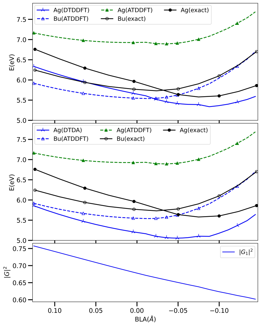
Figure 1: Top panel: 1¹Bu (empty marker) and 2¹Ag (filled marker) excitation energies along the BLA coordinate of trans-butadiene from ATDDFT( 1¹Bu: blue and 2¹Ag: green) within PBE0/cc-pVTZ, “exact” reference $\delta$-CR-EOMCC(2,3) (black), and our DTDDFT_a (blue crosses) curve. Middle panel: Same as in top panel but now showing DTDA_a (blue crosses) 2¹Ag curves. Bottom panel: Norm-square of the eigenvector corresponding to 2¹Ag of Eq. (21) normalized according to Eq. (22).

A key consideration in the DTDDFT computation is the basis-set dependence: the $H_{qD}$ ingredient may potentially increase the basis-set dependence above what ATDDFT typically enjoys. To investigate this, the top panel of Fig. 2 shows the ATDDFT (PBE0) energies of 1¹Bu and 2¹Ag with the basis sets def2-SVP, def2-TZVP, cc-pVDZ, and cc-pVTZ. The results show little difference for either the 1¹Bu or 2¹Ag states across different BLA values. In the second panel, we examine how this behavior changes when replacing the ATDDFT 2¹Ag with its DTDDFT_a counterpart. Notably, DTDDFT_a maintains a comparable level of basis-set dependence to ATDDFT, suggesting robust numerical stability.

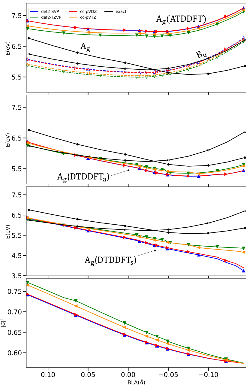
Figure 2: Energies and norm-squares of $G_{I}$ in basis sets def2-SVP(blue), def2-TZVP(green), cc-pVDZ(red) and cc-pVTZ(orange). Top panel: ATDDFT energies of 1¹Bu (empty markers) and 2¹Ag (filled markers) along with the corresponding reference values in black. Second panel: DTDDFT_a 2¹Ag (filled markers). Third panel: DTDDFT_a 2¹Ag (filled markers). Bottom panel: Norm-square, $|G_{I}|$ of the eigenvector corresponding to 2¹Ag.

The third panel shows these same basis sets for the DTDDFT_S variant. First, we notice that although DTDDFT_S would also capture the curve-crossing, it is less accurate than DTDDFT_a, and the trend particularly deviates from the reference towards the negative BLA end of the curve. The figure indicates that this is partly a basis-set non-convergence issue since the results show an increasing sensitivity as the BLA goes from positive values to negative ones. The cc-pVTZ results are likely not quite converged for these larger negative values of the BLA. It is worth noting that the difference between different high-level wavefunction methods also increases as the BLA changes from positive to negative Park et al. (2021). We leave to future work to understand better the underlying cause of this increased sensitivity and deviation of the DTDDFT_S variant at these BLAs. Why the DTDDFT_a variant is more accurate than DTDDFT_S may be understood from the fact that the former accounts for couplings between the KS single excitations in the dressing itself, unlike in DTDDFT_S, which may be important when the single-excitations couple strongly. We further note that DSMA_a outperformed DSMA_S for the lower excitation of the mixed single-double pair in the systems shown in Ref. Dar and Maitra (2023). Finally, we show the $|G|^{2}$ in the above basis sets in the lowest panel. We observe a relatively small basis set dependence especially for negative BLA values; in contrast to the energies, the predicted percentage of single excitations is less sensitive at the negative BLA end than the positive.

III.1 Summary

In conclusion, DTDDFT is an accurate and computationally efficient method for modeling the challenging state of double-excitation character in butadiene, yielding energies much closer to high-level wavefunction reference $\delta-$CR-EOMCC(2,3) of Ref. Park et al. (2021), and better than many other wavefunction methods Park et al. (2021) that much more computationally expensive. The shape of the predicted 2Ag surface through a cut of varying BLA tracks the reference well, and displays the elusive curve-crossing with the 1Bu state at a bond-length close to that of the reference, showing the promise of using DTDDFT for non-adiabatic dynamics calculations of interconversion processes. Whether the entire topology of the conical intersection is well-reproduced will be studied in future work. The underlying character of the state is captured well, as further evidenced by the predicted percentage of single-excitation character, being similar to that from CC3 calculations of Ref. Loos et al. (2019).

Thus, our DTDDFT approach offers a significant advance in the low-cost computational modeling of states of double-excitation character, overcoming key challenges that both ATDDFT and many wavefunction methods suffer from, and offers a more reliable foundation for studying ultrafast dynamics in molecular systems. While our earlier work Dar and Maitra (2023) had demonstrated the fundamental idea of DTDDFT, which in turn had built upon the earlier DTDA Maitra et al. (2004); Cave et al. (2004); Mazur and Włodarczyk (2009); Mazur et al. (2011); Huix-Rotllant et al. (2011) that was unable to correctly yield oscillator strengths and transition densities, here we have shown that DTDDFT can be efficiently extended and implemented to compute excitations involving several single excitations mixing with a double-excitation as in the case of realistic molecules such as the low-lying polyenes. The computational cost is not much beyond ATDDFT, involving only two-electron calculations in a small subspace, and the implementation can be straightforwardly interfaced with standard quantum chemistry codes. This makes it a promising tool for spectra, mapping out excited state potential energy surfaces, and for computing ultrafast non-adiabatic dynamics in photo-excited molecules, an increasingly topical research area.

III.2 Acknowledgment

We thank Piotr Piecuch and Jun Shen for providing us with the BLA data from their work and for useful conversations. We gratefully acknowledge financial support from the National Science Foundation (NSF) under Award No. CHE-2154829 and OAC-2117429, which includes support for the High-Performance Computing Cluster (Price).

III.3 Supplementary

III.3.1 Reduction of DTDDFT kernel to DTDA

Here we show that the dressed frequency-dependent kernels derived above reduce to the DTDA expression from Cave et al. (2004); Mazur and Włodarczyk (2009) when backward transitions are neglected, as in the Tamm-Dancoff approach. We start with the dressing in Eq. 18) but keeping the term, $H_{qD}H_{Dq^{\prime}}$ in the denominator from Eq. (10):

$$X_{qq^{\prime}}(\omega)=\frac{H_{qD}H_{Dq^{\prime}}}{4\sqrt{\nu_{q}\nu_{q^{\prime}}}}\left[1+\frac{(\nu_{q}+\nu_{D})(\nu_{q^{\prime}}+\nu_{D})}{\omega^{2}-(\nu_{D}^{2}+H_{qD}H_{Dq^{\prime}})}\right]\,.$$ (S.23)

Note that the analysis below proceeds similarly for the different variants. The Tamm-Dancoff approximation involves ignoring the backward transitions, i.e. by considering positive-frequencies far from negative-frequency roots. Let us expand around the positive root of the denominator, $\omega_{+}$, where

$$\omega_{+}=\sqrt{\nu_{D}^{2}+H_{qD}H_{Dq^{\prime}}}.$$ (S.24)

Near this root, we express $\omega$ as $\omega_{+}+\delta$, where $\delta$ is a small deviation:

$$\omega=\omega_{+}+\delta.$$ (S.25)

Expanding the denominator in terms of $\delta$ gives, up to order $\delta$:

$$(\omega_{+}+\delta)^{2}-(\nu_{D}^{2}+H_{qD}H_{Dq^{\prime}})=2\omega_{+}\delta\,,$$ (S.26)

so that

$$\frac{1}{\omega^{2}-(\nu_{D}^{2}+H_{qD}H_{Dq^{\prime}})}=\frac{1/2\omega_{+}}{\omega-\omega_{+}}.$$ (S.27)

Assuming the single KS excitation frequencies, $\nu_{q}$ and $\nu_{q^{\prime}}$ lie close to each other and also to the double excitation frequency $\nu_{D}$, the above dressing reduces to

$$X_{qq^{\prime}}(\omega)=\frac{H_{qD}H_{Dq^{\prime}}}{4\nu_{D}}\left[1+\frac{2\nu_{D}^{2}/\omega_{+}}{\left(\omega-\omega_{+}\right)}\right]$$ (S.28)

Near a double excitation, the last term in the brackets becomes much larger than 1, so we can write the above equation as

$$X_{qq^{\prime}}(\omega)=\frac{H_{qD}H_{Dq^{\prime}}(\nu_{D}/\sqrt{\nu_{D}^{2}+H_{qD}H_{Dq^{\prime}}})}{2\left(\omega-\sqrt{\nu_{D}^{2}+H_{qD}H_{Dq^{\prime}}}\right)}.$$ (S.29)

Recalling that $X_{qq^{\prime}}$ is added to the adiabatic part of the xc kernel, we now compare this equation with the kernel given in Ref. Mazur and Włodarczyk (2009), which was derived from the original dressed Tamm-Dancoff approach, and using the analog of what we call here the DTDDFT_S variant. The result from Ref. Mazur and Włodarczyk (2009) is

$$f_{{\scriptscriptstyle\rm XC}\,qq^{\prime}}^{\text{DTDA}}(\omega)=f_{{\scriptscriptstyle\rm XC}\,qq^{\prime}}^{\text{adia}}+\frac{H_{qD}H_{Dq^{\prime}}}{2(\omega-\nu_{D})},$$ (S.30)

from which we see that the dressing term (second term in the above equation) agrees with ours once we replace $\nu_{D}^{2}+H_{qD}H_{Dq^{\prime}}$ to $\nu_{D}^{2}$. As discussed in the main text of the paper, having $H_{qD}H_{Dq^{\prime}}$ in the denominator of the dressing makes it ill-defined by giving it an arbitrary sign-dependence. Here we see another reason to neglect it: ignoring this term makes our kernel agree with the one given in Ref. Mazur and Włodarczyk (2009); Maitra et al. (2004); Cave et al. (2004) derived from the dressed Tamm-Dancoff approach.

References

- Hudson and Kohler (1972) B. S. Hudson and B. E. Kohler, Chemical Physics Letters 14, 299 (1972).
- Schulten and Karplus (1972) K. Schulten and M. Karplus, Chemical Physics Letters 14, 305 (1972).
- Schulten et al. (1976) K. Schulten, I. Ohmine, and M. Karplus, The Journal of Chemical Physics 64, 4422 (1976).
- Andrews and Hudson (1978) J. R. Andrews and B. S. Hudson, The Journal of Chemical Physics 68, 4587 (1978).
- Cave and Davidson (1987) R. J. Cave and E. R. Davidson, Journal of Physical Chemistry 91, 4481 (1987).
- Orlandi et al. (1991) G. Orlandi, F. Zerbetto, and M. Z. Zgierski, Chemical Reviews 91, 867 (1991).
- Fuss et al. (1998) W. Fuss, S. Lochbrunner, A. Müller, T. Schikarski, W. Schmid, and S. Trushin, Chemical Physics 232, 161 (1998).
- Christensen et al. (2004) R. L. Christensen, E. A. Barney, R. D. Broene, M. G. I. Galinato, and H. A. Frank, Archives of biochemistry and biophysics 430, 30 (2004).
- Levine and Martínez (2007) B. G. Levine and T. J. Martínez, Annu. Rev. Phys. Chem. 58, 613 (2007).
- Levine and MartÃnez (2009) B. G. Levine and T. J. MartÃnez, The Journal of Physical Chemistry A 113, 12815 (2009), pMID: 19813720, eprint https://doi.org/10.1021/jp907111u, URL https://doi.org/10.1021/jp907111u.
- Komainda et al. (2013) A. Komainda, B. Ostojic, and H. Köppel, The Journal of Physical Chemistry A 117, 8782 (2013), pMID: 23834412, eprint https://doi.org/10.1021/jp404340m, URL https://doi.org/10.1021/jp404340m.
- Barford (2022) W. Barford, Physical Review B 106, 035201 (2022).
- Papagiannakis et al. (2002) E. Papagiannakis, J. T. Kennis, I. H. van Stokkum, R. J. Cogdell, and R. van Grondelle, Proceedings of the National Academy of Sciences 99, 6017 (2002).
- Ohmine et al. (1978) I. Ohmine, M. Karplus, and K. Schulten, The Journal of Chemical Physics 68, 2298 (1978).
- Lappe and Cave (2000) J. Lappe and R. J. Cave, The Journal of Physical Chemistry A 104, 2294 (2000).
- Loos et al. (2019) P.-F. Loos, M. Boggio-Pasqua, A. Scemama, M. Caffarel, and D. Jacquemin, Journal of Chemical Theory and Computation 15, 1939 (2019), eprint https://doi.org/10.1021/acs.jctc.8b01205, URL https://doi.org/10.1021/acs.jctc.8b01205.
- Park et al. (2021) W. Park, J. Shen, S. Lee, P. Piecuch, M. Filatov, and C. H. Choi, The Journal of Physical Chemistry Letters 12, 9720 (2021).
- Fradelos et al. (2011) G. Fradelos, J. J. Lutz, T. A. Wesołowski, P. Piecuch, and M. Włoch, Journal of Chemical Theory and Computation 7, 1647 (2011).
- Piecuch et al. (2015) P. Piecuch, J. A. Hansen, and A. O. Ajala, Molecular Physics 113, 3085 (2015).
- Runge and Gross (1984) E. Runge and E. K. U. Gross, Phys. Rev. Lett. 52, 997 (1984), URL http://link.aps.org/doi/10.1103/PhysRevLett.52.997.
- Casida (1995) M. Casida, in Recent Advances in Density Functional Methods, Part I, edited by D. Chong (World Scientific, Singapore, 1995).
- Petersilka et al. (1996) M. Petersilka, U. J. Gossmann, and E. K. U. Gross, Phys. Rev. Lett. 76, 1212 (1996), URL http://link.aps.org/doi/10.1103/PhysRevLett.76.1212.
- Tozer et al. (1999) D. J. Tozer, R. D. Amos, N. C. Handy, B. O. Roos, and L. Serrano-Andres, Mol. Phys. 97, 859 (1999).
- Tozer and Handy (2000) D. J. Tozer and N. C. Handy, Phys. Chem. Chem. Phys. 2, 2117 (2000).
- Cave et al. (2004) R. J. Cave, F. Zhang, N. T. Maitra, and K. Burke, Chem. Phys. Lett. 389, 39 (2004), ISSN 0009-2614.
- Casida (2005) M. E. Casida, J. Chem. Phys. 122, 054111 (2005).
- Mazur and Włodarczyk (2009) G. Mazur and R. Włodarczyk, J. Comput. Chem. 30, 811 (2009), ISSN 1096-987X.
- Mazur et al. (2011) G. Mazur, M. Makowski, R. Włodarczyk, and Y. Aoki, Int. J. Quant. Chem. 111, 819 (2011), ISSN 1097-461X.
- Romaniello et al. (2009) P. Romaniello, D. Sangalli, J. A. Berger, F. Sottile, L. G. Molinari, L. Reining, and G. Onida, J. Chem. Phys. 130, 044108 (2009).
- Sangalli et al. (2011) D. Sangalli, P. Romaniello, G. Onida, and A. Marini, The Journal of Chemical Physics 134, 034115 (2011), eprint https://doi.org/10.1063/1.3518705, URL https://doi.org/10.1063/1.3518705.
- Huix-Rotllant et al. (2011) M. Huix-Rotllant, A. Ipatov, A. Rubio, and M. E. Casida, Chem. Phys. 391, 120 (2011), ISSN 0301-0104.
- Casida and Huix-Rotllant (2012) M. Casida and M. Huix-Rotllant, Ann. Rev. Phys. Chem. 63, 287 (2012).
- Casida and Huix-Rotllant (2016) M. E. Casida and M. Huix-Rotllant, Many-Body Perturbation Theory (MBPT) and Time-Dependent Density-Functional Theory (TD-DFT): MBPT Insights About What Is Missing In, and Corrections To, the TD-DFT Adiabatic Approximation (Springer International Publishing, Cham, 2016), pp. 1–60, ISBN 978-3-319-22081-9, URL https://doi.org/10.1007/128_2015_632.
- Maitra (2022) N. T. Maitra, Annual Review of Physical Chemistry 73, 117 (2022), pMID: 34910562, eprint https://doi.org/10.1146/annurev-physchem-082720-124933, URL https://doi.org/10.1146/annurev-physchem-082720-124933.
- Dar and Maitra (2023) D. B. Dar and N. T. Maitra, The Journal of Chemical Physics 159 (2023).
- Maitra et al. (2004) N. T. Maitra, F. Zhang, R. J. Cave, and K. Burke, J. Chem. Phys. 120, 5932 (2004).
- Stein et al. (2009) T. Stein, L. Kronik, and R. Baer, J. Am. Chem. Soc. 131, 2818 (2009).
- Maitra (2016) N. T. Maitra, The Journal of Chemical Physics 144, 220901 (2016), eprint https://doi.org/10.1063/1.4953039, URL https://doi.org/10.1063/1.4953039.
- Maitra (2017) N. T. Maitra, Journal of Physics: Condensed Matter 29, 423001 (2017), URL https://doi.org/10.1088/1361-648x/aa836e.
- Kümmel (2017) S. Kümmel, Advanced Energy Materials 7, 1700440 (2017), eprint https://onlinelibrary.wiley.com/doi/pdf/10.1002/aenm.201700440, URL https://onlinelibrary.wiley.com/doi/abs/10.1002/aenm.201700440.
- Casida (1996) M. E. Casida, in Recent Developments and Applications of Modern Density Functional Theory, edited by J. M. Seminario (Elsevier, Amsterdam, 1996), p. 391.
- Dreuw and Head-Gordon (2005) A. Dreuw and M. Head-Gordon, Chemical reviews 105, 4009 (2005).
- Valiev et al. (2010) M. Valiev, E. Bylaska, N. Govind, K. Kowalski, T. Straatsma, H. V. Dam, D. Wang, J. Nieplocha, E. Apra, T. Windus, et al., Computer Physics Communications 181, 1477 (2010), ISSN 0010-4655, URL http://www.sciencedirect.com/science/article/pii/S0010465510001438.