Near-field dynamical Casimir effect

Abstract

We propose the dynamical Casimir effect in a time-modulated near-field system. The system consists of two bodies made of polaritonic materials, that are brought in close proximity to each other, and the modulation frequency is approximately twice the relevant resonance frequencies of the system. We develop a rigorous fluctuational electrodynamics formalism to explore the produced Casimir flux, associated with the degenerate as well as non-degenerate two-polariton emission processes. We have identified flux contributions from both quantum and thermal fluctuations at finite temperatures, with a dominant quantum contribution even at room temperature under the presence of a strong near-field effect. We have conducted a nonclassicality test for the total radiative flux at finite temperatures, and shown that nonclasscical states of emitted photons can be obtained for a high temperature up to $\sim 250\,$K. Our findings open an avenue for the exploration of dynamical Casimir effect beyond cryogenic temperatures, and may be useful for creating tunable nanoscale nonclassical light sources.

The exploration of fluctuation-induced phenomena in the near-field systems, where at least two bodies are brought in close proximity to each other, has attracted significant interests. Prominent effects in such near-field systems include quantum or thermal Casimir forces Milonni (1994); Lifshitz (1956); Dzyaloshinskii et al. (1961); Mohideen and Roy (1998); M.Bordag et al. (2001); Bressi et al. (2002); Klimchitskaya et al. (2009); Munday et al. (2009); Plunien et al. (1986), where mechanical forces between the bodies can be generated due to quantum or thermal fluctuations, and near-field radiative heat transfer Polder and Van Hove (1971); Carminati and Greffet (1999); Joulain et al. (2005); Kittel et al. (2005); Narayanaswamy et al. (2008); Ben-Abdallah and Biehs (2014); Otey et al. (2010); Kralik et al. (2012); Rousseau et al. (2009); Kim et al. (2015); Zhao et al. (2017); Zhu and Fan (2016); Shi et al. (2015); Bimonte et al. (2017); Ben-Abdallah et al. (2011); Asheichyk and Krüger (2022); Yu et al. (2017) with the heat transfer coefficient between the bodies significantly exceeding the far-field limit. Moreover, while most of the studies on near-field systems focus on systems that are static, in recent years there have been emerging interests in investigating fluctuation physics under the presence of time modulation Khandekar et al. (2015a, b); Buddhiraju et al. (2020); Sloan et al. (2021); Vázquez-Lozano and Liberal (2023); Oue et al. (2023); Yu and Fan (2023, 2024), where the material permittivity is varied as a function of time, with potential applications in cooling and energy harvesting Yu and Fan (2024). In all existing works on time-modulated near-field systems, however, the modulation frequency chosen is significantly smaller compared with the relevant resonance frequencies of the system.

In this work, we consider a time-modulated two-body system composed of two different polaritonic materials, with a modulation frequency that is approximately twice the frequencies of relevant photonic modes supported in the system. We develop a rigorous fluctuational electrodynamics formalism to study both quantum and thermal contributions in the near-field radiative flux between the two bodies. We show that in our time-modulated system the quantum component can dominate over thermal components even at room temperature provided that a strong near-field effect is available. Near-field enhanced degenerate as well as non-degenerate two-polariton emissions can be achieved by tuning the modulation frequency. Furthermore, we consider a nonclassicality test for the total radiative flux at finite temperatures, showing that a nonclasscical state of emitted photons can be obtained for a temperature up to $\sim 250\,$K. Our findings open an avenue for the exploration of dynamical Casimir effect beyond cryogenic temperatures, and may be useful for creating tunable nanoscale nonclassical light sources.

Our work is related to the dynamical Casimir effect that explores photon pair generations from quantum vacuum fluctuations using moving systems Moore (1970); Dodonov et al. (1993); Dalvit et al. (2011). The resulted photon flux is known as Casimir radiation or Casimir flux Kardar and Golestanian (1999); Kenneth and Nussinov (2002). The existing experimental demonstration of dynamical Casimir effect however was carried out in cryogenic temperatures Wilson et al. (2011). The dynamical Casimir effect is also connected to vacuum frictions Pendry (1997); Manjavacas and García de Abajo (2010a, b); Zhao et al. (2012) and the Unruh effect Unruh (1976); Nation et al. (2012). Also, photon-pair generations have been considered in time-varying media Law (1994); Sloan et al. (2021). Such pair generation can lead to the production of two-mode squeezed states Johansson et al. (2010); Wilson et al. (2011); Johansson et al. (2013) which is important for many quantum applications Ralph and Lam (1998); Polzik et al. (1992); Aasi et al. (2013). However, the implication of such pair generation has not been previously studied in time-modulated near-field systems.

Figure 1: (a) Schematic of a planar photonic system composed of two semi-infinitely extended structures separated by a vacuum gap of a separation distance $d=10\,$nm. The upper structure is made of quartz (body 1), whereas in the bottom structure a time-modulated lossless layer is on top of an indium phosphide (InP, body 2) substrate. We assume that the whole system is in thermal equilibrium at a temperature $T$. (b) Dispersion relations of the phonon polartions sustained in the system shown in panel (a). Two flat bands around frequencies $\Omega_{1}$ and $\Omega_{2}$ can be seen. (c) Time modulation, of a modulation frequency $\Omega$, can enable frequency conversion processes from multiple source frequencies $\omega_{l}=\omega+l\Omega$ to the output frequency $\omega$, with $l$ an integer. Conversion processes with $\omega_{l}<0$ (indicated by dashed arrows) will generate the Casimir flux, and all the other processes (indicated by solid arrows) will contribute to the inelastic scattering flux. (d) Net Casimir fluxes $\Phi_{1}^{Q}$ (quantum contribution) and $\Phi_{1}^{T}$ (thermal contribution), as well as inelastic scattering flux $\Upsilon_{1}$, received by body 1 as a function of the modulation frequency $\Omega$ at $T=300\,$K. (e) Time-modulated photon number flux spectra $-F_{1}^{(-1)}$ for three different modulation frequencies which are resonance frequencies labeled in panel (d). The frequency here is for the received photons at body 1.

We consider a time-modulated photonic system composed of two planar structures separated by a vacuum gap of a distance $d=10\,$nm. The upper structure consists of a semi-infinite quartz (body 1, red region) substrate, whereas in the bottom structure a lossless time-modulated layer (green region) with a thickness of 22 nm is located on top of a semi-infinite indium phosphide (InP, body 2, blue region) substrate, as shown in Fig. 1(a). Both quartz and InP support phonon polaritons, and their permittivities are given by da Silva et al. (2012); Palik (1985) $\epsilon_{1,2}(\omega)=\epsilon_{1,2}^{\infty}\left(1+\frac{(\omega_{1,2}^{L})^{2}-(\omega_{1,2}^{T})^{2}}{(\omega_{1,2}^{T})^{2}-\omega^{2}-i\gamma_{1,2}\omega}\right)$ with $\hbar\omega_{1}^{L}=$50 meV, $\hbar\omega_{2}^{L}=$43 meV, $\hbar\omega_{1}^{T}=$49 meV, $\hbar\omega_{2}^{T}=$38 meV, $\hbar\gamma_{1}=$0.26 meV, $\hbar\gamma_{2}=$0.43 meV, $\epsilon_{1}^{\infty}=$2.4, and $\epsilon_{2}^{\infty}=9.6$. The permittivity of the time-modulated layer is given as $\epsilon_{3}(t)=\epsilon_{s}+\delta\epsilon\,{\rm cos}(\Omega t)$, with $\epsilon_{s}=4$ the static permittivity, $\Omega$ the modulation frequency, $\delta\epsilon$ the modulation strength, and $t$ the time. The whole system is translationally invariant in the $x-y$ plane and is assumed to be in thermal equilibrium at a temperature $T$.

Both bodies 1 and 2 support surface phonon polariton modes in the infrared frequency range. The dispersion relation of these modes features two rather flat bands, extending over a broad range of in-plane wavevectors ${\bf k}_{\parallel}\equiv(k_{x},k_{y})$, with frequencies near $\Omega_{1}$ and $\Omega_{2}$, as shown in Fig. 1(b). The modes at $\Omega_{1}$ and $\Omega_{2}$ are mostly confined in body 1 and 2, respectively. In our system, we choose the modulation frequency $\Omega$ to be near the range of $[2\Omega_{1},\,2\Omega_{2}]$. In general, dynamical Casimir effect manifests in terms of the emission of pairs of photons due to modulation. Here, the emission should be strongly enhanced by the presence of the surface phonon polariton Rivera et al. (2019); Sloan et al. (2021).

To illustrate the dynamical Casimir effect in our system, we focus on the net radiative energy flux $Q_{1}$ received by body 1. In the absence of modulation, we have $Q_{1}=0$ since the system is in thermal equilibrium. In the presence of modulation, we have $Q_{1}\neq 0$ and are able to observe signatures of dynamical Casimir effect by analyzing $Q_{1}$. Following a fluctuational electrodynamics formalism Yu and Fan (2023, 2024) for time-modulated radiative energy transfer, $Q_{1}$ can be decomposed into three components as $Q_{1}=\Phi_{1}^{Q}+\Phi_{1}^{T}+\Upsilon_{1}$, where $\Phi_{1}^{Q}$ is the quantum contribution in the Casimir flux, $\Phi_{1}^{T}$ is the thermal contribution in the Casimir flux, and $\Upsilon_{1}$ is the inelastic scattering flux, which has only thermal contribution. These components are given as

$$\Phi_{1}^{Q} =-\int_{0}^{+\infty}d\omega\sum_{l}u(-\omega_{l})\hbar\omega F_{1}^{(l)}(\omega),$$ (1)

$$\Phi_{1}^{T} =-\int_{0}^{+\infty}d\omega\sum_{l}u(-\omega_{l})\hbar\omega\left[n(\omega)+n(-\omega_{l})\right]F_{1}^{(l)}(\omega),$$ (2)

$$\Upsilon_{1} =\int_{0}^{+\infty}d\omega\sum_{l}u(\omega_{l})\hbar\omega\left[n(\omega_{l})-n(\omega)\right]F_{1}^{(l)}(\omega),$$ (3)

where $u(\omega)$ is the Heaviside step function, $n(\omega)=\left[{\rm exp}(\hbar\omega/k_{\rm B}T)-1\right]^{-1}$ is the Bose-Einstein distribution function, $\omega_{l}=\omega+l\Omega$ (with $l$ an integer) is the source frequency, and

$$F_{\beta}^{(l)}(\omega)=\sum_{\alpha,i,j}\frac{2\epsilon_{0}^{2}}{\pi}\frac{1}{A}\epsilon^{\prime\prime}_{\beta}(\omega)\epsilon^{\prime\prime}_{\alpha}(\omega_{l})$$

$$\times\int d{\bf r}_{\beta}\int d{\bf r}_{\alpha}\left|G_{ij}({\bf r}_{\beta},{\bf r}_{\alpha};\omega,\omega_{l})\right|^{2}$$ (4)

with $\alpha,\beta=1,2$ for body 1 or 2, $\epsilon^{\prime\prime}_{\alpha,\beta}(\omega)={\rm Im}\left\{\epsilon_{\alpha,\beta}(\omega)\right\}$, ${\bf r}_{\alpha,\beta}$ the spatial coordinates occupied by body $\alpha$ or $\beta$, and $A$ the surface area of the entire structure in the $x-y$ plane. In Eq. 4, $G_{ij}({\bf r}_{\beta},{\bf r}_{\alpha};\omega,\omega_{l})$, with $i,j=x,y,z$, is the Green’s function for our time-modulated system. The quantity $F_{\beta}^{(l)}$, given in Eq. 4, is the photon number flux spectrum of the frequency conversion process from $\omega_{l}$ to $\omega$. In particular, when $\omega_{l}$ is negative, time modulation introduces mixing between positive (i.e., $\omega$) and negative (i.e., $\omega_{l}$) frequencies, which results in photon pair generations Dodonov et al. (1990); Dodonov and Klimov (1992). Eqs. 1 and 2 describe such pair generation processes, where the photons are generated from quantum and thermal fluctuations, respectively. Other processes, corresponding to the inelastic scattering of existing photons, are included in the inelastic scattering flux, given by Eq. 3, which sources only from thermal fluctuations. All these processes are illustrated in Fig. 1(c).

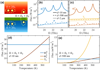
Figure 2: (a) Depending on the resonance condition, a pair of polaritons can be emitted with both of them into either body 1 or 2, or with one into body 1 and the other into body 2. (b,c) Flux components $\Phi_{1}^{Q}$, $\Phi_{1}^{T}$, and $\Upsilon_{1}$ as a function of the modulation frequency $\Omega$ with different separation distances $d$ at $T=300\,$K, where the quantum component ($\Phi_{1}^{Q}$) is shown in panel (b) and the thermal components ($\Phi_{1}^{T}$ and $\Upsilon_{1}$) are shown in panel (c). (d,e) Flux components $\Phi_{1}^{Q}$, $\Phi_{1}^{T}$, and $\Upsilon_{1}$ as a function of temperature $T$ with $d=10\,$nm (d) and $d=500\,$nm (e). The modulation frequency is assumed to be $\Omega_{1}+\Omega_{2}$. Black dashed curves are given by $\Phi_{1}^{Q}\times\left[n(\Omega_{1})+n(\Omega_{2})\right]$.

In Fig. 1(d), we show $\Phi_{1}^{Q}$, $\Phi_{1}^{T}$, and $\Upsilon_{1}$ as a function of the modulation frequency $\Omega$ at $T=300\,$K. The modulation strength is assumed to be $\delta\epsilon=0.4$ throughout this work unless otherwise specified. Three peaks, located at frequencies $\Omega\approx 2\Omega_{2}$, $\Omega_{1}+\Omega_{2}$, and $2\Omega_{1}$, can be found in $\Phi_{1}^{Q}$ (blue curve), each corresponding to a resonance condition for two-polariton generations. Specifically, at $\Omega\approx 2\Omega_{2}$ ($\Omega\approx 2\Omega_{1}$), degenerate generations of two polaritons of the same frequency $\Omega_{2}$ ($\Omega_{1}$) are resonantly enhanced. In contrast, at $\Omega\approx\Omega_{1}+\Omega_{2}$, non-degenerate generations of two polaritons of two different frequencies $\Omega_{1}$ and $\Omega_{2}$ are resonantly enhanced. Similar resonance features can be also seen in the thermal contribution $\Phi_{1}^{T}$ (red curve) of the Casimir flux, since these two terms share the same pair generation mechanism. In contrast, $\Upsilon_{1}$ (orange curve) is featureless, and its magnitude is much smaller than that of the Casimir flux, since the modulation frequency chosen are far from the resonance condition required for the inelastic scattering.

We show in Figs. 1(e) the spectra of $-F_{1}^{(-1)}$ (with $l=-1$), representing the most dominant process. For $\Omega=2\Omega_{2}$, we find three peaks with the dominant one in the middle around the frequency $\Omega_{2}$ (green curve), indicating the dominance of the resonant degenerate two-polariton emission at $\Omega_{2}$. The frequencies of the other two minor peaks are located at $\Omega_{1}$ and $2\Omega_{2}-\Omega_{1}$, respectively, corresponding to a non-degenerate two-polariton emission process. This process is weaker since there is no polariton mode near the frequency of $2\Omega_{2}-\Omega_{1}$. The spectrum for $\Omega=2\Omega_{1}$ (magenta curve) can be similarly interpreted. When $\Omega=\Omega_{1}+\Omega_{2}$, only two peaks, located around $\Omega_{1}$ and $\Omega_{2}$, can be seen, corresponding to a resonant non-degenerate two-polariton emission into the two polariton modes at $\Omega_{1}$ and $\Omega_{2}$, respectively.

In our system, when $\Omega=2\Omega_{1}$ or $2\Omega_{2}$, we expect emission of polariton pairs mainly in body 1 or 2, respectively. In contrast, when $\Omega=\Omega_{1}+\Omega_{2}$, we expect one polariton in the pair should be in body 1 and the other in body 2, as illustrated in Fig. 2(a). Moreover, since these polaritons are strongly confined in either body, we expect the generation process should depend strongly on the separation distance between the bodies. In Fig. 2(b), we show $\Phi_{1}^{Q}$ as a function of the modulation frequency $\Omega$ with different separation distances $d$. The results for $d=10\,$nm (solid curve) are taken from Fig. 1(d). When increasing the separation distance to $d=500\,$nm, one can still observe three peaks but with drastically reduced magnitudes (dashed curve), corresponding to a much weaker resonant enhancement in the two-polariton emission. When further increasing $d$ to $2\,\mu$m, the peak features largely disappear, thus demonstrating a strong near-field effect in producing two-polariton emission into body 1. Note that a frequency shift of the resonance peaks can be seen when varying $d$ because the polariton dispersion changes as $d$ varies. As shown in Fig. 2(c), similar observations can be found in $\Phi_{1}^{T}$ (red curves) as $d$ changes at a temperature of $T=300\,$K. Here, at room temperature, the magnitude of $\Phi_{1}^{T}$ is smaller than that of $\Phi_{1}^{Q}$. In contrast, $\Upsilon_{1}$ decreases more mildly as $d$ increases and shows no resonance features for all separation distances, as shown by the orange curves in Fig. 2(c). As mentioned above, here the inelastic scattering is an off-resonance process. Thus the polariton response, which dominates in the near field, is not the key contributing factor here. Noticeably, $\Upsilon_{1}$ dominates over both $\Phi_{1}^{Q}$ and $\Phi_{1}^{T}$ at a large separation distance $d=2\,\mu$m.

In Figs. 2(d,e), we show $\Phi_{1}^{Q}$, $\Phi_{1}^{T}$, and $\Upsilon_{1}$ as a function of temperature $T$ with $\Omega=\Omega_{1}+\Omega_{2}$ for two different separation distances. For $d=10\,$nm [Fig. 2(d)], in the temperature range under study, $\Upsilon_{1}$ (orange curve) is much smaller than the other two components, as also demonstrated in Fig. 1(d). $\Phi_{1}^{Q}$ (blue curve) is independent on the temperature because it origins from quantum fluctuations, whereas $\Phi_{1}^{T}$ (red curve) shows strong temperature dependence and becomes dominant over $\Phi_{1}^{Q}$ only when $T\apprge 480\,$K. These results demonstrate that the quantum contribution $\Phi_{1}^{Q}$ can dominate over all other contributions in the near-field regime. In contrast, when increasing the separation distance to $d=500\,$nm, $\Upsilon_{1}$ can be dominant over both $\Phi_{1}^{Q}$ and $\Phi_{1}^{T}$ when $T\apprge 292\,$K, as shown in Fig. 2(e), and $\Phi_{1}^{Q}$ is no longer dominant. Noticeably, as shown in Figs. 2(d,e), $\Phi_{1}^{T}$ can be simply reproduced by $\Phi_{1}^{Q}\times\left[n(\Omega_{1})+n(\Omega_{2})\right]$, given by the black dashed curves, which highlights the underlining mechanism of non-degenerate two-polariton emissions for both $\Phi_{1}^{Q}$ and $\Phi_{1}^{T}$. Also, as shown in Figs. 2(d,e), both $\Phi_{1}^{T}$ and $\Upsilon_{1}$ vanish at zero temperature because they both source from thermal fluctuations.

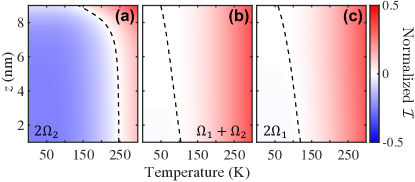
Figure 3: Normalized quantum-classical indicator $\mathcal{I}$ as a function of temperature $T$ and vertical distance $z$ measured from the top of the time-modulated layer, for the system considered in Fig. 1. Normalized $\mathcal{I}$ is evaluated within the vacuum gap for three different modulation frequencies $\Omega=2\Omega_{2}$ (a), $\Omega_{1}+\Omega_{2}$ (b), and $2\Omega_{1}$ (c), as indicated in Fig. 1(d). Black dashed curves indicate $\mathcal{I}=0$. The regions of nonclassical radiations locate on the left-hand side of the black dashed curves, where $\mathcal{I}<0$.

In the dynamical Casimir effect, the generation of correlated photon pairs can lead to two-mode squeezing Wilson et al. (2011). Two-mode squeezed states can also be generated with thermal vacuum Lee (1990). Inspired by these works, here we study the quantum nature of the emitted radiative flux by conducting a nonclassicality test for our system shown in Fig. 1. For a Hermitian operator $\hat{\bf h}^{\dagger}\cdot\hat{\bf h}$, with $\hat{\bf h}$ composed of creation and annihilation operators, one can show, by using the Glauber-Sudarshan P function, that any classical state of fields satisfies Miranowicz et al. (2010) $\langle:\hat{\bf h}^{\dagger}\cdot\hat{\bf h}:\rangle\geq 0$, where $::$ denotes normal ordering. Here for $\hat{\bf h}$ we consider the two-mode quadrature operator $\hat{\bf h}_{\theta}$, which is given as Miranowicz et al. (2010)

$$\hat{\bf h}_{\theta}= \frac{1}{\sqrt{8\pi\epsilon_{0}\hbar}}\left[e^{i\theta}\hat{{\bf E}}({\bf r},\omega_{-})+e^{-i\theta}\hat{{\bf E}}^{\dagger}({\bf r},\omega_{-})\right.$$

$$\left.+ie^{i\theta}\hat{{\bf E}}({\bf r},\omega_{+})-ie^{-i\theta}\hat{{\bf E}}^{\dagger}({\bf r},\omega_{+})\right].$$ (5)

In Eq. 5, $\theta$ is the angle that defines the principal squeezing axis, $\hat{{\bf E}}({\bf r},\omega_{-})$ and $\hat{{\bf E}}({\bf r},\omega_{+})$ represent the electric field operators for the two modes evaluated at two frequencies $\omega_{-}=\frac{\Omega}{2}-\delta\omega$ and $\omega_{+}=\frac{\Omega}{2}+\delta\omega$, respectively, with $\omega_{-}+\omega_{+}=\Omega$. The variable ${\bf r}$ represents the spatial coordinate inside the vacuum gap. Note that for $\delta\omega\rightarrow 0$, $\hat{\bf h}_{\theta}$ can be used to characterize the degenerate two-mode squeezing (i.e., $\omega_{-}=\omega_{+}$). We define the quantum-classical indicator $\mathcal{I}$ as Miranowicz et al. (2010)

$$\mathcal{I}=\min_{\theta}\langle:\hat{\bf h}^{\dagger}_{\theta}\cdot\hat{\bf h}_{\theta}:\rangle=C({\bf r},T)-|B({\bf r},T)|.$$ (6)

Here $C({\bf r},T)=\sum_{M=\pm}R({\bf r};\omega_{M},\omega_{M})n(\omega_{M})$ and $B({\bf r},T)=\sum_{M=\pm}R({\bf r};\omega_{M}-\Omega,\omega_{M})[2n(\omega_{M})+1]$ with

$$R({\bf r};\omega,\omega^{\prime})=\sum_{\alpha,i,j}\epsilon^{\prime\prime}_{\alpha}(\omega^{\prime})$$

$$\times\int d{\bf r}_{\alpha}{G}_{ij}({\bf r},{\bf r}_{\alpha};\omega,\omega^{\prime}){G}^{*}_{ij}({\bf r},{\bf r}_{\alpha};\omega^{\prime},\omega^{\prime}),$$

where the superscript * denotes the complex conjugate operation. Note that $C({\bf r},T)$ is a real positive quantity.

In Eq. 6, $C({\bf r},T)$ arises from the inelastic scattering flux, whereas $B({\bf r},T)$ arises from the Casimir flux, containing both thermal and quantum components, the presence of which is essential to reach the nonclassicality condition

$$C({\bf r},T)<|B({\bf r},T)|,$$ (7)

leading to $\mathcal{I}<0$. In Figs. 3(a-c), we show the normalized quantum-classical indicator $\mathcal{I}/{\mathcal{N}}$, with ${\mathcal{N}}=\sum_{M=\pm}R({\bf r};\omega_{M},\omega_{M})/2$, as a function of temperature $T$ and vertical distance $z$ measured from the top of the time-modulated layer, for the system considered in Fig. 1. The normalized quantum-classical indicator is evaluated within the vacuum gap for three different modulation frequencies (see labels inside). In Figs. 3(a) and (c), we have $\delta\omega=0$ for degenerate two-mode squeezing, whereas $\delta\omega=(\Omega_{1}-\Omega_{2})/2$ for non-degenerate two-mode squeezing in Fig. 3(b). As shown in Figs. 3(a-c), the state of the emitted photon flux can exhibit nonclassical behaviors even at finite temperatures. The behaviors change from nonclassical to classical when increasing the temperature for all three modulation frequencies due to an increased thermal noise. Moreover, there is also a spatial dependence in the state of the radiation. Away from the time-modulated layer (i.e, as $z$ increases), the nonclassical behavior is weaker since the effect of modulation is weaker, as shown in Figs. 3(a-c). Moreover, when $\Omega=2\Omega_{2}$ [Fig. 3(a)], there is a larger parameter range where nonclassical behaviors can be observed, since the time-modulated layer is attached to body 2 and the degenerate two-mode squeezing at $\Omega_{2}$ is more efficient. In this case, the nonclassical behavior can survive up to a temperature of $\sim 250\,$K.

In summary, we have shown that a strong dynamical Casimir effect can be obtained in a time-modulated near-field polaritonic system composed of two bodies, which results in near-field enhanced degenerate and non-degenerate two-polariton generations. The two-polariton generation is manifested as a photon flux, named Casimir flux, which has contributions from both quantum and thermal fluctuations at finite temperatures. Noticeably, the quantum components can dominate over all the other thermal components even at room temperature when a strong near-field effect due to the excitation of polaritons is present. We have conducted the nonclassicality test for the total radiative flux at finite temperatures, and shown that nonclasscical states of emitted photons can be obtained even for a high temperature up to $\sim 250\,$K. Our findings may be of importance for developing tunable nanoscale nonclassical light sources, and may motivate further explorations for quantum applications based on thermal light.

This work has been supported by a MURI program from the U. S. Army Research Office (Grant No. W911NF-19-1-0279).

References

- Milonni (1994) P. W. Milonni, The quantum vacuum: an introduction to quantum electrodynamics (Academic Press, San Diego, 1994).
- Lifshitz (1956) E. M. Lifshitz, Sov. Phys. JETP 52, 73 (1956).
- Dzyaloshinskii et al. (1961) I. E. Dzyaloshinskii, E. M. Lifshitz, and L. P. Pitaevskii, Advances in Physics 10, 165 (1961).
- Mohideen and Roy (1998) U. Mohideen and A. Roy, Phys. Rev. Lett. 81, 4549 (1998).
- M.Bordag et al. (2001) M.Bordag, U. Mohideen, and V. M. Mostepanenko, Phys. Rep. 353, 1 (2001).
- Bressi et al. (2002) G. Bressi, G. Carugno, R. Onofrio, and G. Ruoso, Phys. Rev. Lett. 88, 41804 (2002).
- Klimchitskaya et al. (2009) G. Klimchitskaya, U. Mohideen, and V. Mostepanenko, Reviews of Modern Physics 81, 1827 (2009).
- Munday et al. (2009) J. N. Munday, F. Capasso, and V. A. Parsegian, Nature 457, 170 (2009).
- Plunien et al. (1986) G. Plunien, B. Müller, and W. Greiner, Physics Reports 134, 87 (1986).
- Polder and Van Hove (1971) D. Polder and M. Van Hove, Phys. Rev. B 4, 3303 (1971).
- Carminati and Greffet (1999) R. Carminati and J. J. Greffet, Phys. Rev. Lett. 82, 1660 (1999).
- Joulain et al. (2005) K. Joulain, J.-P. Mulet, F. Marquier, R. Carminati, and J.-J. Greffet, Surface Science Reports 57, 59 (2005).
- Kittel et al. (2005) A. Kittel, W. Müller-Hirsch, J. Parisi, S. A. Biehs, D. Reddig, and M. Holthaus, Phys. Rev. Lett. 95, 224301 (2005).
- Narayanaswamy et al. (2008) A. Narayanaswamy, S. Shen, and G. Chen, Phys. Rev. B 78, 115303 (2008).
- Ben-Abdallah and Biehs (2014) P. Ben-Abdallah and S.-A. Biehs, Phys. Rev. Lett. 112, 044301 (2014).
- Otey et al. (2010) C. R. Otey, W. T. Lau, S. Fan, et al., Physical Review Letters 104, 154301 (2010).
- Kralik et al. (2012) T. Kralik, P. Hanzelka, M. Zobac, V. Musilova, T. Fort, and M. Horak, Physical Review Letters 109, 224302 (2012).
- Rousseau et al. (2009) E. Rousseau, A. Siria, G. Jourdan, S. Volz, F. Comin, J. Chevrier, and J. J. Greffet, Nat. Photon. 3, 514 (2009).
- Kim et al. (2015) K. Kim, B. Song, V. Fernández-Hurtado, W. Lee, W. Jeong, L. Cui, D. Thompson, J. Feist, M. H. Reid, F. J. García-Vidal, et al., Nature 528, 387 (2015).
- Zhao et al. (2017) B. Zhao, B. Guizal, Z. M. Zhang, S. Fan, and M. Antezza, Phys. Rev. B 95, 245437 (2017).
- Zhu and Fan (2016) L. Zhu and S. Fan, Phys. Rev. Lett. 117, 134303 (2016).
- Shi et al. (2015) J. Shi, B. Liu, P. Li, L. Y. Ng, and S. Shen, Nano Lett. 15, 1217 (2015).
- Bimonte et al. (2017) G. Bimonte, T. Emig, M. Kardar, and M. Krüger, Annual Review of Condensed Matter Physics 8, 119 (2017).
- Ben-Abdallah et al. (2011) P. Ben-Abdallah, S. A. Biehs, and K. Joulain, Phys. Rev. Lett. 107, 114301 (2011).
- Asheichyk and Krüger (2022) K. Asheichyk and M. Krüger, Phys. Rev. Lett. 129, 170605 (2022).
- Yu et al. (2017) R. Yu, A. Manjavacas, and F. J. García de Abajo, Nat. Commun. 8, 2 (2017).
- Khandekar et al. (2015a) C. Khandekar, A. Pick, S. G. Johnson, and A. W. Rodriguez, Phys. Rev. B 91, 115406 (2015a).
- Khandekar et al. (2015b) C. Khandekar, Z. Lin, and A. W. Rodriguez, Applied Physics Letters 106, 151109 (2015b).
- Buddhiraju et al. (2020) S. Buddhiraju, W. Li, and S. Fan, Physical Review Letters 124, 077402 (2020).
- Sloan et al. (2021) J. Sloan, N. Rivera, J. D. Joannopoulos, and M. Soljačić, Physical Review Letters 127, 053603 (2021).
- Vázquez-Lozano and Liberal (2023) J. E. Vázquez-Lozano and I. Liberal, Nature Communications 14, 4606 (2023).
- Oue et al. (2023) D. Oue, K. Ding, and J. Pendry, Physical Review A 107, 063501 (2023).
- Yu and Fan (2023) R. Yu and S. Fan, Phys. Rev. Lett. 130, 096902 (2023).
- Yu and Fan (2024) R. Yu and S. Fan, Proceedings of the National Academy of Sciences 121, e2401514121 (2024).
- Moore (1970) G. T. Moore, Journal of Mathematical Physics 11, 2679 (1970).
- Dodonov et al. (1993) V. Dodonov, A. Klimov, and D. Nikonov, Physical Review A 47, 4422 (1993).
- Dalvit et al. (2011) D. A. R. Dalvit, P. A. M. Neto, and F. D. Mazzitelli, Fluctuations, Dissipation and the Dynamical Casimir Effect (Springer-Verlag, Berlin, 2011), pp. 419–457.
- Kardar and Golestanian (1999) M. Kardar and R. Golestanian, Rev. Mod. Phys. 71, 1233 (1999).
- Kenneth and Nussinov (2002) O. Kenneth and S. Nussinov, Phys. Rev. D 65, 085014 (2002).
- Wilson et al. (2011) C. M. Wilson, G. Johansson, A. Pourkabirian, M. Simoen, J. R. Johansson, T. Duty, F. Nori, and P. Delsing, Nature 479, 376 (2011).
- Pendry (1997) J. B. Pendry, J. Phys. Condens. Matter 9, 10301 (1997).
- Manjavacas and García de Abajo (2010a) A. Manjavacas and F. J. García de Abajo, Phys. Rev. Lett. 105, 113601 (2010a).
- Manjavacas and García de Abajo (2010b) A. Manjavacas and F. J. García de Abajo, Phys. Rev. A 82, 063827 (2010b).
- Zhao et al. (2012) R. Zhao, A. Manjavacas, F. J. García de Abajo, and J. B. Pendry, Phys. Rev. Lett. 109, 123604 (2012).
- Unruh (1976) W. G. Unruh, Physical Review D 14, 870 (1976).
- Nation et al. (2012) P. Nation, J. Johansson, M. Blencowe, and F. Nori, Reviews of Modern Physics 84, 1 (2012).
- Law (1994) C. Law, Physical Review A 49, 433 (1994).
- Johansson et al. (2010) J. Johansson, G. Johansson, C. Wilson, and F. Nori, Physical Review A 82, 052509 (2010).
- Johansson et al. (2013) J. Johansson, G. Johansson, C. Wilson, P. Delsing, and F. Nori, Physical Review A 87, 043804 (2013).
- Ralph and Lam (1998) T. C. Ralph and P. K. Lam, Physical Review Letters 81, 5668 (1998).
- Polzik et al. (1992) E. Polzik, J. Carri, and H. Kimble, Physical Review Letters 68, 3020 (1992).
- Aasi et al. (2013) J. Aasi, J. Abadie, B. Abbott, R. Abbott, T. Abbott, M. Abernathy, C. Adams, T. Adams, P. Addesso, R. Adhikari, et al., Nature Photonics 7, 613 (2013).
- da Silva et al. (2012) R. E. da Silva, R. Macêdo, T. Dumelow, J. Da Costa, S. Honorato, and A. Ayala, Physical Review B 86, 155152 (2012).
- Palik (1985) E. D. Palik, Handbook of Optical Constants of Solids (Academic Press, San Diego, 1985).
- Rivera et al. (2019) N. Rivera, T. Christensen, and P. Narang, Nano Letters 19, 2653 (2019).
- Dodonov et al. (1990) V. Dodonov, A. Klimov, and V. Man’Ko, Physics Letters A 149, 225 (1990).
- Dodonov and Klimov (1992) V. Dodonov and A. Klimov, Physics Letters A 167, 309 (1992).
- Lee (1990) C. T. Lee, Physical Review A 42, 4193 (1990).
- Miranowicz et al. (2010) A. Miranowicz, M. Bartkowiak, X. Wang, Y.-x. Liu, and F. Nori, Physical Review A 82, 013824 (2010).
- Scheel and Buhmann (2008) S. Scheel and S. Y. Buhmann, acta physica slovaca 58, 675 (2008).