High-Dimensional Gaussian Process Regression with
Soft Kernel Interpolation
Chris Camaño* Daniel Huang*
California Institute of Technology ccamano@caltech.edu San Francisco State University danehuang@sfsu.edu
Abstract
We introduce soft kernel interpolation (SoftKI) designed for scalable Gaussian Process (GP) regression on high-dimensional datasets. Inspired by Structured Kernel Interpolation (SKI), which approximates a GP kernel via interpolation from a structured lattice, SoftKI approximates a kernel via softmax interpolation from a smaller number of learned interpolation (i.e., inducing) points. By abandoning the lattice structure used in SKI-based methods, SoftKI separates the cost of forming an approximate GP kernel from the dimensionality of the data, making it well-suited for high-dimensional datasets. We demonstrate the effectiveness of SoftKI across various examples, and demonstrate that its accuracy exceeds that of other scalable GP methods when the data dimensionality is modest (around ).
1 Introduction
Gaussian processes (GPs) are flexible function approximators based on Bayesian inference. However, there are scalability concerns. For a dataset comprising data points, constructing the covariance matrix required for GP inference incurs a space complexity of , and solving the associated linear system for exact posterior inference and hyperparameter optimization via direct methods requires time complexity. These computational costs render exact GP inference challenging, even for modest , though efforts have been made to accelerate exact GP inference Wang et al., (2019); Gardner et al., (2021).
One approach to constructing scalable GP algorithms is based on inducing points (e.g., see Quinonero-Candela and Rasmussen, (2005) and Snelson and Ghahramani, (2005)). Intuitively, a set of inducing points forms a representative subset of the original dataset. Given inducing points, we can form a low-rank approximation of the original GP kernel to construct an approximate GP which reduces the time complexity of posterior inference to . However, the limitation of using inducing points means that the model may not accurately approximate the full kernel if the selected inducing points are not sufficiently representative of the entire dataset.
Another approach is based on Structured Kernel Interpolation (SKI) Wilson and Nickisch, (2015) and its variants such as product kernel interpolation Gardner et al., (2018) and Simplex-SKI Kapoor et al., (2021). SKI approximates a GP kernel via interpolation from a pre-computed and dense rectilinear grid of inducing points. Structured interpolation enables fast matrix-vector multiplications (MVMs), which can be leveraged to scale inference by using the conjugate gradient (CG) method to solve for the inversion of the approximate kernel matrix. Importantly, SKI supports a larger number of inducing points than many other approximate GPs since it is applicable even when there is not low-rank structure in the true kernel. However, this approach also causes the time complexity of posterior inference to become dependent on the dimensionality of the data (e.g., for a MVM in SKI and for a MVM in Simplex-SKI). This motivates us to search for accurate and scalable GP regression algorithms that can scale to larger while retaining the benefits of kernel interpolation.
In this paper, we introduce soft kernel interpolation (SoftKI), which combines aspects of inducing points and SKI to enable scalable GP regression on high-dimensional data sets. SoftKI retains SKI’s insight that a kernel can be well-approximated via interpolation. However, we opt to learn the locations of the interpolation points as in an inducing point approach. Our main observation is that while SKI can support large numbers of interpolation points, it uses them in a sparse manner—only a few interpolation points contribute to the interpolated value of any single data point. Consequently, we should still be able to interpolate successfully provided that we place enough inducing points in good locations relative to the dataset at hand, i.e., learn their locations. The code can be found at https://github.com/danehuang/softki.
This change removes the explicit dependence of the cost of the method on the data dimensionality , but at the cost of disrupting the structure of the kernel, motivating the need for an alternative inference method. We show how to recover efficient and accurate inference by interpolating from a softmax of learned interpolation points, hence the name soft kernel interpolation (Section 1 and Section 4.2). The time complexity of posterior inference is and the space complexity is (Section 4.3). Additionally, SoftKI can leverage GPU acceleration and supports stochastic optimization for scalability. We evaluate SoftKIs on a variety of datasets from the UCI repository Kelly et al., (2017) and show that it is more accurate in test Root Mean Square Error (RMSE) compared to popular scalable GP methods based on inducing points when the data dimensionality is modest (around ) and also scalable to larger than methods based on SKI (Section 5). We also evaluate SoftKI on high-dimensional molecule datasets ( in the hundreds to thousands) and show its superior performance.
2 Background
Notation. We will write a list of vectors as the flattened length- vector so that , i.e., is a vector where indices to exclusive is . The notation maps a function across a flattened list of vectors. Uppercase boldface letters denote matrices. We will sometimes use the notation to define a matrix by defining its th and th entry. For example, defines a matrix whose -th and -th entry .
2.1 Gaussian processes
A (centered) Gaussian process (GP) is a random function . It has jointly Gaussian finite-dimensional distributions so that
| (1) |
for any where is a positive semi-definite function called a kernel function and indicates a Gaussian distribution with mean and kernel matrix (also called covariance matrix).
To perform GP regression on the labeled dataset , we assume the data is generated as follows:
| (GP) | ||||
| (likelihood) |
where is a function sampled from a GP and each observation is evaluated at perturbed by independent and identically distributed (i.i.d.) Gaussian noise with zero mean and variance . The posterior predictive distribution has the closed-form solution Rasmussen and Williams, (2005)
| (2) |
where . Using standard direct methods, the time complexity of inference is which is the complexity of solving the system of linear equations in variables
| (3) |
for so that the posterior mean (2) is .
A GP’s hyperparameters include the noise and other parameters such as those involved in the definition of a kernel such as its lengthscale and scale . Thus . The hyperparameters can be set by maximizing the log-marginal likelihood of a GP
| (4) |
where is notation for the probability density function (PDF) of a Gaussian distribution with mean and covariance and we have explicitly indicated the dependence of and on . For simplicity, we will abbreviate and leave the dependence on hyperparameters implicit.
2.2 Sparse Gaussian Process Regression.
Many scalable GP methods address the high computational cost of GP inference by approximating the kernel using a Nyström method Williams and Seeger, (2000). This approach involves selecting a smaller set of inducing points, , to serve as representatives for the complete dataset. The original kernel is then approximated as:
| (5) |
leading to an overall inference complexity of .
Over the last two decades, Nyström approximation for GP kernels has been refined and adapted in various ways, with many improvements driven by a theoretical re-characterization of inducing points as inducing variables and the limitations of the Nyström approximation as a standalone approximation of the true covariance Quinonero-Candela and Rasmussen, (2005). These ideas were crystallized into the widely used SGPR method Titsias, (2009), which combines Nyström GP kernel approximation with a variational optimization process. To perform SGPR, we use the following generative process:
| (SGPR) | ||||
| (likelihood) |
where are inducing variables and is a set of inducing points. We will abbreviate . Observe that so that a SGPR reduces to GP regression after marginalizing out the inducing variables . In SGPR, inference is directly performed with the inducing variables since marginalization would lead to an expensive computation. Consequently, we need a procedure for selecting the inducing points .
Towards this end, Titsias, (2009) introduces a variational distribution and solves for the that minimizes the KL divergence . The optimal is
| (6) |
where . This maximizes the evidence lower bound (ELBO)
| (7) |
where is a Nyström approximation of . Since the ELBO is a lower bound on the log-marginal likelihood , we can maximize the ELBO via gradient based optimization as a proxy for maximizing to learn the location of the inducing points by treating it as a GP hyperparmeter, i.e., . The time complexity of computing the ELBO is .
Given learned inducing points, the posterior predictive distribution has closed form
| (8) |
The time complexity of posterior inference is since it requires solving
| (9) |
for which is dominated by forming .
2.3 Structured Kernel Interpolation.
SKI approaches scalable GP regression by approximating a large covariance matrix by interpolating from cleverly chosen inducing points. In particular, SKI makes the approximation
| (10) | ||||
| (11) | ||||
| (12) | ||||
| (13) |
where is a sparse matrix of interpolation weights, , and . The posterior predictive distribution is then the standard GP posterior predictive
| (14) |
where is replaced with . SKI uses linear CG to solve the linear system
| (15) |
for . Since the time complexity of CG depends on access to fast MVMs, SKI makes two design choices that are compatible with CG. First, SKI uses cubic interpolation Keys, (1981) weights so that has four non-zero entries in each row, i.e., is sparse. Second, SKI chooses the inducing points to be on a fixed rectilinear grid in which induces multilevel Toeplitz structure in if is a stationary kernel.
Putting the two together, the resulting is a structured kernel which enables fast MVMs. If we wish to have distinct inducing points for each dimension, the grid will contain inducing points leading to a total complexity of GP inference of since there are nonzero entries per row of and a MVM with a Toeplitz structured kernel like can be done in time via a Fast Fourier Transform (FFT) Wilson, (2014). Thus, for low dimensional problems, SKI can provide significant speedups compared to vanilla GP inference and supports a larger number of inducing points compared to SGPR.
3 Related work
Beyond SGPR and vanilla SKI, a wide range of approximate GP models and variants have been developed that align closely with SoftKI.
Building on SGPR, Stochastic Variational Gaussian Processes (SVGP) Hensman et al., (2013) extends the optimization process used for SGPR to use stochastic variational inference. This further reduces the computational cost of GP inference to since optimization is now over a variational distribution on , rather than the full posterior. Importantly SVGP is highly scalable to GPUs since its optimization strategy is amenable to minibatch optimization procedures.
Variants of Structured Kernel Interpolation. While SKI can provide significant speedups over vanilla GP inference, its scaling restricts its usage to low-dimensional settings where . To address this, Gardner et al., (2018) introduced SKIP, which optimizes SKI by expressing a -dimensional kernel as a product of one-dimensional kernels. This reduces MVM costs from to , using grid points per component kernel instead of . However, SKIP is limited to dimensions to for large datasets, as it requires substantial memory and may suffer from low-rank approximation errors.
Recent work on improving the scaling properties of SKI has been focused on efficient incorporation of simplicial interpolation, which when implemented carefully in the case of Simplex-GP Kapoor et al., (2021) and Sparse grid GP Yadav et al., (2023) can reduce the cost of a single MVM with an down to . These methods differ in the grid construction used for interpolation with Simplex-SKI opting for a permutohedral lattice Adams et al., (2010), while sparse grid-GP uses sparse grids and a bespoke recursive MVM algorithm, leading to MVM costs of and respectively. While both of these methods greatly improve the scaling of SKI, they still feature a problematic dependency on limiting their extension to arbitrarily large datasets.
4 Method
In this section, we introduce SoftKI (Algorithm 1). To construct a SoftKI, we will take the same starting point as SKI, namely that
| (16) |
can be used as an approximation of . However, we will deviate in that we will abandon the structure given by a lattice and opt to learn the locations of the interpolation points instead. This raises several issues. First, we revisit the choice of interpolation because we have changed the locations of the interpolation points (Section 1). Second, we require an efficient procedure for learning the inducing points (Section 4.2). Third, we require an alternative route to recover a scalable GP since our approach removes structure in the kernel that was used in SKI for efficient inference (Section 4.3).
4.1 Soft Kernel Interpolation
Whereas a cubic (or higher-order) interpolation scheme is natural in SKI when using a static lattice structure, our situation is different since the locations of the interpolation points are dynamic. In particular, we would ideally want our interpolation scheme to have the flexibility to adjust the contributions of inducing points used to interpolate a kernel value in a data-dependent manner. To accomplish this, we propose softmax interpolation weights.
Definition 4.1 (Softmax interpolation weights).
Define softmax interpolation weights as the following matrix
| (17) |
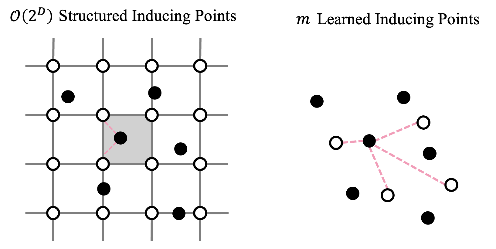
Since a softmax can be interpreted as a probability distribution, we can view SoftKI as interpolating from a probabilistic mixture of inducing points. Softmax interpolation ensures that each input point is interpolated from all inducing points, with an exponential weighting favoring closer points. As a result, we obtain a matrix where each row represents the softmax interpolation weights between a single point and all inducing points (Figure 1). Since softmax interpolation continuously assigns weights over each inducing point for each , the resulting matrix is not strictly sparse. However, as increases the weights for distant points become negligible. This leads to an effective sparsity, with each predominantly influenced only by its nearest inducing points during reconstruction of .
4.2 Learning Inducing Points
Similar to a SGPR, we can treat the inducing points as hyper parameters of a GP and learn them by optimizing an appropriate objective. We propose optimizing the marginal log likelihood for a SoftKI which has closed form solution
| (18) |
Each evaluation of has time complexity and space complexity where is the number of interpolation points. However, this is tractable to compute only when because is low-rank. We thus propose to learn inducing points by maximizing with a method based on gradient descent. In our experience a direct implementation of (18) is prone to numerical instability since it is possible for to only be approximately psd (See Appendix B.1 ).
Hutchinson’s Pseudoloss. To address this problem, we compute a pseudo-marginal log likelihood following Maddox et al., (2022), which was originally used to stabilize GP regression in low precision settings. The main idea is to construct a such that . In this way, a gradient-based optimization scheme can still optimize the GP hyperparameters as if the exact marginal log likelihood was used.
Let where we have explicitly indicated the dependence on the GP hyperparameters .
Definition 4.2 (Hutchinson Pseudoloss).
The Hutchinson Pseudoloss is defined as
| (19) |
where are Gaussian random vectors normalized to have unit length, and are solutions to the equations
| (20) |
The gradient of w.r.t. the hyperparameters is
| (21) | |||
| (22) | |||
| (23) |
so that it is approximately equivalent to the gradient of w.r.t. the hyperparameters estimated with Hutchinson’s trace estimator Girard, (1989); Hutchinson, (1989); Gibbs and MacKay, (1996).
Stochastic optimization. For further stability, we perform minibatch gradient descent on the Hutchinson pseudoloss (see line 7 of Algorithm 1). We emphasize that we are performing stochastic gradient descent and not stochastic variational inference as in SVGP Hensman et al., (2013). In particular, we do not define a distribution on nor make a variational approximation. Our experiments (Section 5) show that this approach works well in practice.
4.3 Posterior Inference
Because is low-rank, we can use the matrix inversion lemma to rewrite the posterior predictive of SoftKI as
| (24) |
where (see Appendix A). To perform posterior mean inference, we solve
| (25) |
for weights . Note that this is the posterior mean of a SGPR with replaced with and replaced with . Moreover, note that is with replaced with . Since is a matrix, the solution of the system of linear equations has time complexity . The formation of requires the multiplication of a matrix with a matrix which has time complexity . Thus the complexity of SoftKI posterior mean inference is since it is dominated by the formation of .
Solving with QR. Unfortunately, solving (25) for can be numerically unstable. Foster et al., (2009) introduce a stable QR solver approach for a Subset of Regressors (SoR) GP Smola and Bartlett, (2000) which we adapt to a SoftKI.
Define a matrix
| (26) |
where is the Cholesky decomposition of so that
| (27) |
Let be the the QR decomposition of so that is a orthogonal matrix and is right triangular matrix. Then
| (28) | ||||
| (29) | ||||
| (30) |
is a solution to . We thus solve for . For additional experiments demonstrating the inability of other linear solvers to offer comparable accuracy to the QR-stabilized solve detailed in this section, see Appendix B.3.
| n | d | SoftKI-512 | SGPR-512 | SVGP-1024 | |
|---|---|---|---|---|---|
| 3droad | 391386 | 3 | 0.605 0.0 | - | 0.496 0.001 |
| Kin40k | 36000 | 8 | 0.237 0.008 | 0.205 0.008 | 0.192 0.006 |
| Protein | 41157 | 9 | 0.649 0.01 | 0.66 0.009 | 0.659 0.008 |
| Houseelectric | 1844352 | 11 | 0.064 0.001 | - | 0.071 0.0 |
| Bike | 15641 | 17 | 0.204 0.006 | 0.284 0.002 | 0.268 0.003 |
| Elevators | 14939 | 18 | 0.389 0.01 | 0.401 0.007 | 0.389 0.009 |
| Keggdirected | 43944 | 20 | 0.081 0.005 | 0.096 0.007 | 0.088 0.005 |
| Pol | 13500 | 26 | 0.195 0.006 | 0.261 0.008 | 0.3 0.005 |
| Keggundirected | 57247 | 27 | 0.115 0.004 | 0.126 0.005 | 0.127 0.007 |
| Buzz | 524925 | 77 | 0.253 0.002 | - | 0.296 0.0 |
| Song | 270000 | 90 | 0.793 0.004 | - | 0.803 0.004 |
| Slice | 48150 | 385 | 0.049 0.003 | 0.479 0.027 | 0.127 0.001 |
| n | d | SoftKI-512 | SVGP-512 | SVGP-1024 | |
|---|---|---|---|---|---|
| 3droad | 391386 | 3 | 25.159 0.667 | 29.043 0.336 | 35.646 0.492 |
| Kin40k | 36000 | 8 | 2.327 0.149 | 2.792 0.09 | 3.421 0.038 |
| Protein | 41157 | 9 | 2.625 0.15 | 3.03 0.075 | 3.762 0.037 |
| Houseelectric | 1844352 | 11 | 118.355 0.856 | 137.845 1.217 | 168.461 1.77 |
| Bike | 15641 | 17 | 0.96 0.008 | 1.224 0.116 | 1.456 0.028 |
| Elevators | 14939 | 18 | 0.972 0.07 | 1.11 0.005 | 1.383 0.033 |
| Keggdirected | 43944 | 20 | 2.86 0.052 | 3.233 0.054 | 4.051 0.021 |
| Pol | 13500 | 26 | 0.84 0.032 | 1.039 0.037 | 1.304 0.017 |
| Keggundirected | 57247 | 27 | 3.545 0.098 | 4.269 0.055 | 5.231 0.06 |
| Buzz | 524925 | 77 | 37.166 0.195 | 40.015 0.695 | 49.109 0.319 |
| Song | 270000 | 90 | 19.45 0.203 | 20.45 0.141 | 25.012 0.042 |
| Slice | 48150 | 385 | 3.869 0.044 | 3.78 0.054 | 4.715 0.068 |
| n | d | SoftKI-512 | SGPR-512 | SVGP-1024 | |
|---|---|---|---|---|---|
| Ac-ala3-nhme | 76598 | 126 | 0.67 0.006 | 0.861 0.006 | 0.859 0.005 |
| Dha | 62777 | 168 | 0.592 0.004 | 0.899 0.012 | 0.902 0.011 |
| Stachyose | 24544 | 261 | 0.372 0.004 | 0.68 0.003 | 0.613 0.002 |
| At-at | 18000 | 354 | 0.459 0.012 | 0.594 0.011 | 0.644 0.012 |
| At-at-cg-cg | 9137 | 354 | 0.398 0.006 | 0.595 0.03 | 0.569 0.039 |
| Buckyball-catcher | 5491 | 444 | 0.245 0.017 | 0.776 0.011 | 0.468 0.048 |
| Double-walled-nanotube | 4528 | 1110 | 0.105 0.004 | 1.001 0.048 | 0.518 0.036 |
5 Experiments
We compare the performance of SoftKIs against popular scalable GPs on selected data sets from the UCI data set repository Kelly et al., (2017), a common GP benchmark (Section 5.1). Next, we test SoftKIs on high-dimensional molecule data sets from the domain of computational chemistry (Section 5.2). Finally we explore the role of noise in a SoftKI and discuss best practices (Section 5.3).
5.1 Benchmark on UCI Regression
We evaluate the efficacy of a SoftKI against other scalable GP methods on data sets of varying size and data dimensionality from the UCI repository Kelly et al., (2017). We choose SGPR and SVGP as two scalable GP methods since these methods can be applied in a relatively blackbox fashion, and thus, can be applied to many data sets.
Hardware details. We run all experiments on a single Nvidia RTX 3090 GPU which has 24Gb of VRAM. A GPU with more VRAM can support larger datasets. Our machine uses an Intel i9-10900X CPU at 3.70GHz with 10 cores. This primarily affects the timing of SoftKI and SVGP which use batched hyperparameter optimization, and thus, move data on and off the GPU more frequently than SGPR.
Experiment details. For this experiment, we split the data set into for training and for testing. We standardize the data to have mean and standard deviation using the training data set. We use a radial basis function (RBF) kernel with a single learnable lengthscale for all dimensions and a learnable output scale. We choose inducing points for SoftKI. Following Wang et al., (2019), we use for SGPR and for SVGP. We learn model hyperparameters for SoftKI by maximizing the marginal log likelihood, and for SGPR and and SVGP by maximizing the ELBO. However, we opt to not learn the noise for SoftKI instead fixing the value as which is explained further in Section 5.3.
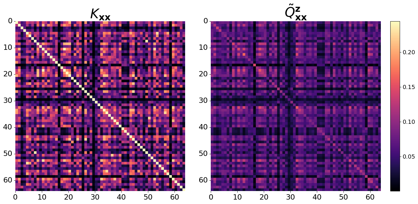
We perform iterations of training using the Adam optimizer Kingma and Ba, (2014) for all methods with a learning rate of . The learning rate for SGPR is since we are not performing batching. We use a default implementation of SGPR and SVGP from GPyTorch. For SoftKI and SVGP, we use a minibatch size of . We report the average test RMSE and hyperparameter optimization time for each method across three seeds. A visualization of the learned kernel for the elevators dataset is given in Figure 2.
Accuracy. Table 1 compares the test RMSE of various GP models trained on the UCI data set. We observe that SoftKI’s have competitive and/or more accurate test RMSE compared to SGPR or SVGP when the data dimensionality is modest (around ). This holds on all data sets that we have tested. For low-dimensional datasets such as 3droad, SoftKI performs poorly. SKI performs well on these low-dimensional datasets.
Timing. Table 2 compares the average training time per epoch in seconds to for hyperparameter optimization of SoftKI vs SVGP. We do not include SGPR since it is much faster but does not support batched stochastic optimization, and thus, is limited to smaller datasets. We observe that SVGP and SoftKI have similar performance characteristics due to the mini-batch gradient descent approach that both SVGP and SoftKI employ. SVGP requires slightly more compute since it additionally learns the parameters of a variational Gaussian distribution. We include both 512 and 1024 inducing points for SVGP for a fair timing comparison with SoftKI, although the test RMSE performance for SVGP is better with 1024 inducing points.
5.2 High-Dimensional Molecule Dataset
Since SoftKI’s are performant on large dimensional data sets from the UCI repository, we also test the performance on molecular potential energy surface data. These datasets have high dimensionality.
Dataset details. The MD22 Chmiela et al., (2023) data set consists of biomolecules ranging from 42 atoms to 370 atoms and their properties. More concretely, we have a labeled data set where encodes the Cartesian coordinates of the atomic nuclei in the bio-molecule in Ångström’s and encodes the energy of the bio-molecule in kcal/mol. The dimensionality of is where is the number of atoms in the bio-molecule since each atom takes 3 coordinates to describe in -space. For example, a atom system will have . We consider all available molecules.
Experiment details. For consistency, we keep the experimental setup the same as for UCI regression. In particular, we still use the RBF kernel and not a molecule-specific kernel that incorporates additional information such as the atomic number of each atom (e.g., a Hydrogen atom) or invariances (e.g., rotational invariance). We standardize the data set to have mean and standard deviation . We note that in an actual application of GP regression to this setting, we may only opt to center the targets to be mean . This is because energy is a relative number that can be arbitrarily shifted, whereas scaling the distances between atoms will affect the physics.
Accuracy. Table 3 compares the test RMSE of various GP models trained on MD22. We see that SoftKI is by far the most performant approximate GP method. GPs that fit forces have been successfully applied to fit such data sets to chemical accuracy. In our case, we do not fit derivative information. It would be an interesting direction of future work to extend SoftKI to handle derivatives. Notably, GP regression with derivative information results in covariance matrices, posing additional scaling challenges with and .
5.3 The Role of the Noise Hyperparameter
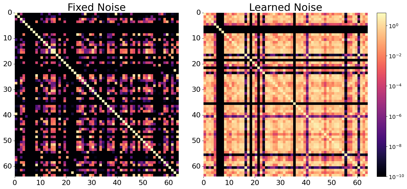
The noise hyper parameter is typically learned jointly with the other GP hyper parameters when performing GP regression. However, in our experience we achieve lower RMSE by fixing to a small value instead, e.g., . We hypothesize that this is because a learned noise parameter can interfere with learning the locations of the inducing points. In Figure 3, we show the log entries of for keggdirected (). We see that the fixed noise kernel has smaller entries compared to the kernel with learned noise. A smaller entry means that a pair of inducing points and are more dissimilar for fixed noise kernels compared to kernels with learned noise. In other words, they are further apart in data space w.r.t. the kernel. Since we seek to learn optimal placements for a set of inducing points this behavior can be understood as inducing points independently mapping the data space instead of clustering together. We observe that the gap in performance diminishes as the dimensionality increases. This matches our understanding of distances in high-dimensional spaces which are larger, and thus, more dissimilar.For additional details on the RMSE impact of learning noise, as well as the effect of increasing or decreasing the total number of inducing points used in SoftKI (see Appendix B.2 and Appendix B.4).
6 Conclusion
In this paper, we introduce SoftKI designed for GP regression on large and high-dimensional datasets. SoftKI combines aspects of SKI and inducing points methods to retain the benefits of kernel interpolation while also scaling to higher dimensional datasets. We have tested SoftKI on a variety of datasets from the UCI repository and shown that it outperforms other scalable GP methods. We have also demonstrated the superior performance of SoftKI on molecular data, a high-dimensional dataset.
Acknowledgements Chris Camaño acknowledges support by the National Science Foundation Graduate Research Fellowship under Grant No. 2139433. Additionally, we would like to extend our appreciation to Ethan N. Epperly for his thoughtful comments and advice on this work.
References
- Adams et al., (2010) Adams, A., Baek, J., and Davis, M. (2010). Fast high-dimensional filtering using the permutohedral lattice. Comput. Graph. Forum, 29:753–762.
- Chmiela et al., (2023) Chmiela, S., Vassilev-Galindo, V., Unke, O. T., Kabylda, A., Sauceda, H. E., Tkatchenko, A., and Müller, K.-R. (2023). Accurate global machine learning force fields for molecules with hundreds of atoms. Science Advances, 9(2):eadf0873.
- Foster et al., (2009) Foster, L., Waagen, A., Aijaz, N., Hurley, M., Luis, A., Rinsky, J., Satyavolu, C., Way, M. J., Gazis, P., and Srivastava, A. (2009). Stable and efficient gaussian process calculations. Journal of Machine Learning Research, 10(31):857–882.
- Gardner et al., (2021) Gardner, J. R., Pleiss, G., Bindel, D., Weinberger, K. Q., and Wilson, A. G. (2021). Gpytorch: Blackbox matrix-matrix gaussian process inference with gpu acceleration.
- Gardner et al., (2018) Gardner, J. R., Pleiss, G., Wu, R., Weinberger, K. Q., and Wilson, A. G. (2018). Product kernel interpolation for scalable gaussian processes.
- Gibbs and MacKay, (1996) Gibbs, M. N. and MacKay, D. J. C. (1996). Efficient implementation of Gaussian processes for interpolation.
- Girard, (1989) Girard, A. (1989). A fast ‘monte-carlo cross-validation’ procedure for large least squares problems with noisy data. Numer. Math., 56(1):1–23.
- Hensman et al., (2013) Hensman, J., Fusi, N., and Lawrence, N. D. (2013). Gaussian processes for big data. arXiv preprint arXiv:1309.6835.
- Hutchinson, (1989) Hutchinson, M. (1989). A stochastic estimator of the trace of the influence matrix for laplacian smoothing splines. Communication in Statistics- Simulation and Computation, 18:1059–1076.
- Kapoor et al., (2021) Kapoor, S., Finzi, M., Wang, K. A., and Wilson, A. G. G. (2021). Skiing on simplices: Kernel interpolation on the permutohedral lattice for scalable gaussian processes. In International Conference on Machine Learning, pages 5279–5289. PMLR.
- Kelly et al., (2017) Kelly, M., Longjohn, R., and Nottingham, K. (2017). The uci machine learning repository. https://archive.ics.uci.edu.
- Keys, (1981) Keys, R. (1981). Cubic convolution interpolation for digital image processing. IEEE Transactions on Acoustics, Speech, and Signal Processing, 29(6):1153–1160.
- Kingma and Ba, (2014) Kingma, D. P. and Ba, J. (2014). Adam: A method for stochastic optimization. arXiv preprint arXiv:1412.6980.
- Maddox et al., (2022) Maddox, W. J., Potapcynski, A., and Wilson, A. G. (2022). Low-precision arithmetic for fast gaussian processes. In Uncertainty in Artificial Intelligence, pages 1306–1316. PMLR.
- Quinonero-Candela and Rasmussen, (2005) Quinonero-Candela, J. and Rasmussen, C. E. (2005). A unifying view of sparse approximate gaussian process regression. The Journal of Machine Learning Research, 6:1939–1959.
- Rasmussen and Williams, (2005) Rasmussen, C. E. and Williams, C. K. I. (2005). Gaussian Processes for Machine Learning (Adaptive Computation and Machine Learning). The MIT Press.
- Smola and Bartlett, (2000) Smola, A. and Bartlett, P. (2000). Sparse greedy gaussian process regression. In Leen, T., Dietterich, T., and Tresp, V., editors, Advances in Neural Information Processing Systems, volume 13. MIT Press.
- Snelson and Ghahramani, (2005) Snelson, E. and Ghahramani, Z. (2005). Sparse gaussian processes using pseudo-inputs. Advances in neural information processing systems, 18.
- Titsias, (2009) Titsias, M. (2009). Variational learning of inducing variables in sparse gaussian processes. In Artificial intelligence and statistics, pages 567–574. PMLR.
- Wang et al., (2019) Wang, K. A., Pleiss, G., Gardner, J. R., Tyree, S., Weinberger, K. Q., and Wilson, A. G. (2019). Exact gaussian processes on a million data points.
- Williams and Seeger, (2000) Williams, C. K. I. and Seeger, M. (2000). Using the nyström method to speed up kernel machines. In Proceedings of the 13th International Conference on Neural Information Processing Systems, NIPS’00, page 661–667, Cambridge, MA, USA. MIT Press.
- Wilson and Nickisch, (2015) Wilson, A. and Nickisch, H. (2015). Kernel interpolation for scalable structured gaussian processes (kiss-gp). In International conference on machine learning, pages 1775–1784. PMLR.
- Wilson, (2014) Wilson, A. G. (2014). Covariance kernels for fast automatic pattern discovery and extrapolation with Gaussian processes. PhD thesis, University of Cambridge Cambridge, UK.
- Yadav et al., (2023) Yadav, M., Sheldon, D., and Musco, C. (2023). Kernel interpolation with sparse grids.
Appendix A SoftKI Posterior Predictive Derivation
We first recall how to apply the matrix inversion lemma to the posterior mean of a GP.
Lemma A.1 (Matrix inversion with GPs).
| (31) |
Proof.
| (identity) | ||||
| (mult by ) | ||||
| (rearrange) | ||||
| (mult both sides by on left) | ||||
| (defn ) | ||||
| (factor) | ||||
| (matrix inversion lemma) | ||||
| (mult on right) |
∎
Now, we extend the matrix inversion lemma to SoftKI.
Lemma A.2 (Matrix inversion with interpolation).
| (32) |
Proof.
Recall . The result follows by applying Lemma A.1 with replaced with . ∎
Appendix B Additional Experiments
In this section, we examine the influence of various aspects of the SoftKI model and its sensitivity to algorithm design decisions made throughout the paper.
In Section B.1, we discuss the rationale behind using a stochastic trace estimation scheme for computing the marginal log likelihood during stochastic optimization. Sections B.2 and B.4 provide further insights into the model’s dependence on the noise hyperparameter and the effect of the number of inducing points. Lastly, B.3 motivates choice of linear solver, comparing the use alternative linear solvers for the posterior inference procedure described in. Section 4.3.
B.1 Effect of Hutchinson Pseudoloss
| N | D | |||
|---|---|---|---|---|
| 3droad | 391386 | 3 | 0.605 0.0 | - |
| Kin40k | 36000 | 8 | 0.237 0.008 | 0.24 0.0 |
| Protein | 41157 | 9 | 0.649 0.01 | - |
| Houseelectric | 1844352 | 11 | 0.064 0.001 | - |
| Bike | 15641 | 17 | 0.204 0.006 | 0.203 0.006 |
| Elevators | 14939 | 18 | 0.389 0.01 | 0.389 0.01 |
| Keggdirected | 43944 | 20 | 0.081 0.005 | 0.081 0.005 |
| Pol | 13500 | 26 | 0.195 0.006 | 0.193 0.006 |
| Keggundirected | 57247 | 27 | 0.115 0.004 | - |
| Buzz | 524925 | 77 | 0.254 0.0 | 0.248 0.001 |
| Song | 270000 | 90 | 0.793 0.005 | 0.793 0.004 |
| Slice | 48150 | 385 | 0.049 0.003 | 0.024 0.005 |
In Section 4.2, we advocate for the use of the Hutchinson pseudoloss to overcome numerical stability issues that arise when calculating the exact marginal log likelihood. This adjustment is specifically to address situations where the matrix is not psd. In other approximate GP model using gpytorch, this challenge is typically met by performing a Cholesky decomposition followed by an efficient low-rank computation of the log determinant through the matrix determinant lemma. In our experience even when using versions of the Cholesky decomposition that add additional jitter along the diagonal there are still situations where can be poorly conditioned. The Hutchinson pseudoloss offers a more stable alternative because it does not rely on the matrix being positive semi-definite.
In Table 4 we replicate the UCI experiment of Section 5.1 using the Hutchinson pseudoloss and the exact marginal log likelihood . For most situations the exact marginal log likelihood produces a lower test RMSE rsult than the Hutchinson pseudoloss, however for some datasets that produce noisy the method can crash due to the Cholesky decomposition failing.
Hutchinson pseudoloss involves computing solutions to the equations
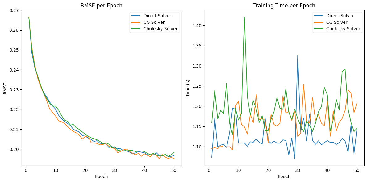
where is the covariance matrix parameterized by GP hyperparameters , is the target vector, and are unit length normalized Gaussian random vectors. In most implementations, these systems are typically solved using CG solvers due to their efficiency with large, sparse systems. However, during the training of a SoftKI, the matrices involved are relatively small because of the mini-batching strategy employed (See Algorithm 1). This makes direct solvers more efficient and attractive in practice. Figure 4 illustrates the impact of different linear solvers for this task, comparing CG, a direct solver, and a Cholesky decomposition routine.
In this example, we set the tolerance of the CG solver to to achieve accuracy comparable to that of a direct solve. Following the approach outlined by Gardner et al. Gardner et al., (2021), we employ a rank-10 pivoted Cholesky preconditioner. Additionally, we incorporate the CG stabilization modifications proposed by Maddox et al in Maddox et al., (2022). All three approaches exhibited roughly similar behavior, with the direct solver running slightly faster than the alternatives. We suspect this performance gain is due to low-level optimizations in the underlying numerical linear algebra package used for direct linear solves.
B.2 Additional Experiments for the Noise Hyperparameter
| N | D | Learn | ||
|---|---|---|---|---|
| 3droad | 391386 | 3 | 0.605 0.0 | 0.728 0.001 |
| Kin40k | 36000 | 8 | 0.237 0.008 | 0.385 0.004 |
| Protein | 41157 | 9 | 0.649 0.01 | 0.725 0.004 |
| Houseelectric | 1844352 | 11 | 0.064 0.001 | 0.072 0.001 |
| Bike | 15641 | 17 | 0.204 0.006 | 0.245 0.002 |
| Elevators | 14939 | 18 | 0.389 0.01 | 0.393 0.005 |
| Keggdirected | 43944 | 20 | 0.081 0.005 | 0.083 0.005 |
| Pol | 13500 | 26 | 0.195 0.006 | 0.235 0.006 |
| Keggundirected | 57247 | 27 | 0.115 0.004 | 0.118 0.004 |
| Buzz | 524925 | 77 | 0.254 0.0 | 0.262 0.004 |
| Song | 270000 | 90 | 0.793 0.005 | 0.791 0.005 |
| Slice | 48150 | 385 | 0.049 0.003 | 0.051 0.003 |
As we discussed in Section 5.3, the noise hyperparameter plays a delicate role in the performance of a SoftKI. Earlier we argued that allowing the noise hyperparameter to be learned jointly with other hyperparameters can negatively affect the final test RMSE of the model. To investigate this further, we revisited the UCI benchmark, this time treating the noise as a learnable parameter, while keeping all other settings aligned with the original experiement setting. The results, summarized in Table 5, demonstrate that for most datasets allowing the model to learn the noise negatively impacts the the final RMSE.
B.3 Alternative Methods for Posterior Inference
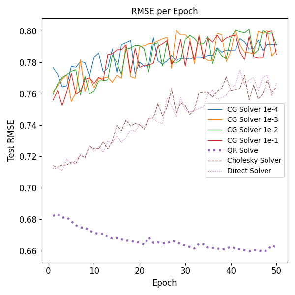
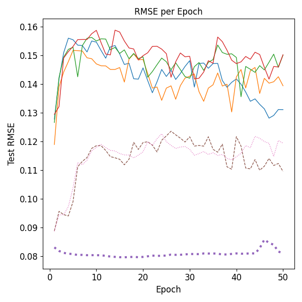
Section 4.3 details the adaptation of the QR stabilized linear solve for approximate kernels Foster et al., (2009) to the SoftKI setting. In this section, we provide empirical evidence illustrating how other linear solvers fail when confronted with datasets that generate noisy kernels. We focus on two datasets, protein and keggundirected, which have previously caused instability in the Hutchinson pseudoloss computation.
As a reminder the QR stabilized linear solve is motivated by the challenge of solving the linear system:
| (33) |
where is the estimated (potentially noisy) kernel matrix , and is the interpolated kernel between inducing points and training points .
In this example we evaluate a direct solver, the Cholesky decomposition method, and CG with convergence tolerances set to , , , and . Despite adjusting the tolerances for the CG method, our experiments revealed that all solvers—except for the QR-stabilized routine—resulted in training instability. Figure 5 depicts the test RMSE performance across the different solvers. The direct and Cholesky solvers, while more stable than the CG solvers, failed to produce reliable solutions. Similarly, the CG method did not converge to acceptable solutions within the tested tolerance levels. In contrast, the QR-stabilized solver consistently produced stable and accurate solutions justifying its choice as a correctional measure that stabilizes a SoftKI on difficult problems.
B.4 The Effect of Inducing Points
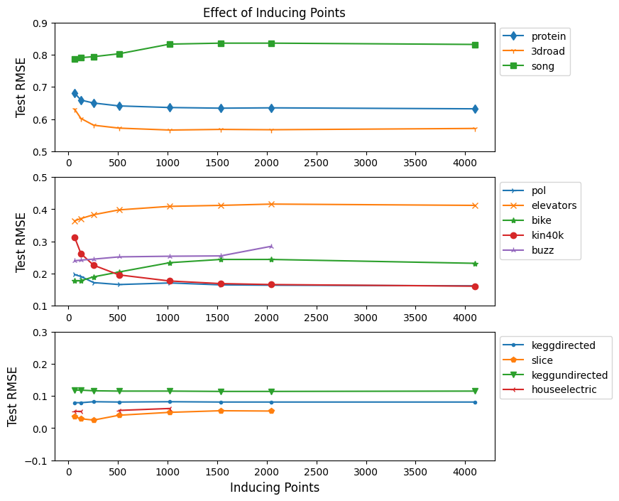
Figure 3 illustrates the effect of the number of inducing points on the test RMSE of SoftKI. We find that increasing the number of inducing points is helpful for improving test RMSE performance on some datasets (e.g., kin40k and pol) while it is detrimental for other datasets (e.g., elevators and bike). While it would stand to reason that increasing the number of inducing points would improve performance (up to a certain point), it is not clear to us why increasing the number of inducing points would be detrimental in some cases. We do not observe over fitting in the test RMSE curves but see saturation at a higher test RMSE. It would be an interesting direction of future work to investigate this phenomenon and how to improve it.