Observable-projected ensembles

Abstract

Measurements in many-body quantum systems can generate non-trivial phenomena, such as preparation of long-range entangled states, dynamical phase transitions, or measurement-altered criticality. Here, we introduce a new measurement scheme that produces an ensemble of mixed states in a subsystem, obtained by measuring a local Hermitian observable on part of its complement. We refer to this as the observable-projected ensemble. Unlike standard projected ensembles—where pure states are generated by projective measurements on the complement—our approach involves projective partial measurements of specific observables. This setup has two main advantages: theoretically, it is amenable to analytical computations, especially within conformal field theories. Experimentally, it requires only a linear number of measurements, rather than an exponential one, to probe the properties of the ensemble. As a first step in exploring the observable-projected ensemble, we investigate its entanglement properties in conformal field theory and perform a detailed analysis of the free compact boson.

1 Introduction

In recent years quantum dynamics involving measurements has drawn a lot of attention in the literature, driven by multiple factors. First of all, any interaction of a quantum computer with a classical observer will include a measurement. With the ever-growing number of quantum-computing experiments, it is hard to overestimate the importance of this. For instance, performing measurements on a subsystem of a resource state can be used to prepare non-trivial quantum states with long-range correlations, and this is the basis of measurement-based quantum computation [1, 2, 3, 4, 5, 6, 7]. On a more fundamental level, the dynamics with measurement can exhibit a rich phase structure [8, 9, 10, 11, 12, 13, 14, 15, 16, 17, 18], which in some cases can be explained by an emergent quantum error correction in an ensemble of states [19]. Moreover, measurements can be used to alter the pristine entanglement properties of critical states [20, 21, 22, 23, 24, 25, 26], as well as to uncover the intricate inner structure of pure states, which is the subject of this paper.

Projected ensembles: Given a system $A\cup\overline{A}$, if the state $|\Psi\rangle$ is the result of a unitary evolution, at late times, the local stationary behavior is described by a statistical ensemble, corresponding to a thermal or generalized Gibbs ensemble for chaotic or integrable systems, respectively [27, 28]. This implies that the reduced density matrix $\rho_{A}=\mathrm{Tr}_{\overline{A}}|\Psi\rangle\langle\Psi|$ is the main conceptual tool to understand how and in which sense an isolated quantum system can be described by a mixed state at large times. A natural definition that arises from the reduced density matrix is a family of entanglement measures, the Rényi entropies, which are given by

$$S_{A}^{(n)}=\frac{1}{1-n}\log\operatorname*{Tr}[\rho_{A}^{n}],\qquad S_{A}^{(1)}=-\operatorname*{Tr}[\rho_{A}\log\rho_{A}].$$ (1)

The right part of the equation above is the definition of the von Neumann entanglement entropy, one of the most successful entanglement measures, which can be derived by doing an analytic continuation in $n$ of $S_{A}^{(n)}$ and then taking the limit $n\to 1$ [29].

The question of whether the thermalization is even approximately true or not, and how to properly describe it, has been the focus of quantum statistical mechanics. The above statement, however, raises questions about the coarse-grained nature of $A$: if we average over the state of $\overline{A}$, what is the most appropriate way to describe the state of $A$? Modern quantum experiments have put forward a new perspective, in which one can consider a projected ensemble of pure states corresponding to different microscopic states of $\overline{A}$: given a set of states $|z_{i}\rangle$ in $\overline{A}$, we define the projected ensemble $\mathcal{E}$ of states of $A$ as

$$\mathcal{E}=\{p_{i},\ |\Psi_{i}\rangle=p_{i}^{-1/2}\langle z_{i}|\Psi\rangle\},$$ (2)

where $p_{i}=|\langle z_{i}|\Psi\rangle|^{2}$ are the corresponding probabilities of finding $\overline{A}$ in the state $|z_{i}\rangle$ . Then, for a complete set of states of $\overline{A}$, the average state $|\Psi_{i}\rangle$ reduces to $\rho_{A}$, since

$$\rho_{1}=\mathbb{E}_{\mathcal{E}}|\Psi_{i}\rangle\langle\Psi_{i}|=\sum_{i}p_{i}|\Psi_{i}\rangle\langle\Psi_{i}|=\sum_{i}\langle z_{i}|\Psi\rangle\langle\Psi|z_{i}\rangle=\operatorname*{Tr}_{\overline{A}}|\Psi\rangle\langle\Psi|.$$ (3)

However, a similar operation is far from trivial if we consider the higher moments of $\mathcal{E}$, i.e. averaging $(|\Psi_{i}\rangle\langle\Psi_{i}|)^{\otimes k}$. Indeed, one main feature of the projected ensemble is its convergence to a uniform distribution over the set of pure states in $A$, the Haar ensemble, for chaotic dynamics and infinite-temperature initial states. This phenomenon has been dubbed deep thermalization and it represents a form of equilibration in quantum many-body systems stronger than the regular thermalization we mentioned above, which only constrains the expectation values of observables over the ensemble of the stationary state [30, 31]. It has been also proven in different setups like free fermionic systems [32], deep random circuits [30, 33], dual-unitary models [34, 35, 36, 37, 38], and then also extended to finite temperature cases [39, 33]. Nevertheless, beyond dynamical settings, the ground state properties of the ensemble (2) have not been further studied so far. To the best of our knowledge, the main features one can derive about $\mathcal{E}$ after a complete set of measurements is that, if $|\Psi\rangle$ is an infinite temperature state, then $\mathcal{E}$ is the Haar ensemble, while at finite temperature $\mathcal{E}$ is the Scrooge ensemble (a deformation of the Haar random ensemble [40]) corresponding to the appropriate thermal reduced density matrix. The goal of this paper is to investigate more projected ensembles originating from the ground states.

Entanglement after partial projective measurements:

Despite studying the static properties of $\mathcal{E}$ is challenging, focusing on specific measurement outcomes is more accessible for analytical computations. For instance, many interesting quantum many-body systems in 1+1 dimensions possess quantum critical points whose ground state can be described by conformal field theories (CFT) at long distances, and there has been a moderate progress in describing post-measurement states $|\Psi_{i}\rangle$ of CFT using the boundary CFT (BCFT) description [41, 42]. Unfortunately, these are applicable only by choosing the basis and the outcome $|z_{i}\rangle$ in a way that the induced boundary condition on $B$ is still conformally invariant. For instance, we can measure the transverse magnetization in the XX spin chain (aka free fermionic model) and post-select a measurement outcome. In the absence of a magnetic field, the most likely outcome is an antiferromagnetic string. It is expected that this case leads to the Dirichlet boundary condition in the bosonization language and so it is related to the BCFT. More generally, the main result about specific measurement outcomes is that, after partial projective measurements, if $B$ is a subsystem of length $s$ in an infinite system, $A$ is a region of length $\ell$ adjacent to $B$, and $\epsilon$ is a UV cutoff, then the Rényi entanglement entropies behave, at leading order, as [41]

$$S^{(n)}_{A}=\frac{c}{12}\frac{n+1}{n}\log\frac{\ell(\ell+s)}{s\epsilon}+\log b_{0}$$ (4)

where $c$ is the central charge of the CFT and $\log b_{0}$ is the Affleck-Ludwig boundary term. This result has been generalized to several different geometries, including cases where $B$ is not a simply connected region. We can recognize in Eq. (4) the leading order behavior of the entanglement entropy in the presence of a boundary. However, not all the measurement outcomes lead to conformal invariant boundary conditions. For instance, if we post-select the ferromagnetic string, it does not lead to a BCFT, because it already breaks the $U(1)$ symmetry [43, 44]. The challenging part of this problem is not only the extension to the non-conformal invariant setups, but also the computations of quantities like the localizable entanglement [45] or the measurement induced entanglement (MIE) [46]. The latter is defined for a tripartite geometry, $A_{1},A_{2}$ and $B$, where we projectively measure $B$ and the MIE between $A_{1}$ and $A_{2}$ is defined as

$$\mathrm{MIE}(A_{1}:A_{2})=\sum_{i}p_{i}S^{(1)}_{A_{1}}(|\Psi_{i}\rangle)\qquad S^{(1)}_{A_{1}}(|\Psi_{i}\rangle)=-\mathrm{Tr}\rho_{A_{1}}\log\rho_{A_{1}}.$$ (5)

Here $i$ parameterize the measurement outcomes with probabilities $p_{i}$ and $\rho_{A_{1}}=\mathrm{Tr}_{A_{2}}|\Psi_{i}\rangle\langle\Psi_{i}|$. Since both the MIE and the localizable entanglement involve a sum of all possible measurement outcomes, it is hard to analytically predict their behavior, since we do not have a closed formula for each $S^{(1)}_{A_{1}}$ in a field theory setup. However, the MIE can be used to gain insights about the initial state $|\Psi\rangle$, for example, the sign structure of stabilizer states [46], or whether measurements can generate entanglement between distant parties without the need for direct interaction.

Main results:

Even though a lot of effort has been done to understand the out-of-equilibrium properties of projected ensembles, finding result in the ground state of critical theories is far from being trivial due to the main challenges we summarized above.

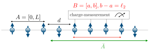
Figure 1: The geometry we consider in this manuscript is the following: we measure an observable (such as the charge operator) in a region $B$ and we study the properties of the reduced density matrix $\rho_{A}$ after this operation.

The focus of this paper is exactly to approach the structure of a projected ensemble using a field-theoretic framework. Fortunately, oftentimes we are not interested in the state of the system after a complete projection of its subsystem $B$: in general there are exponentially many (in the size of $B$) outcomes, so sampling from this ensemble is hard. In contrast, measuring a certain observable inside $B$ will lead to a number of outcomes that scale at most linearly with the size. This is why in this paper we will introduce a smaller ensemble which corresponds to projecting on a particular value of an extensive observable, rather than a complete projective measurement of $B$. As we will see, such an ensemble has an elegant field-theoretic description. Specifically, we will consider a local Hermitian operator $\mathcal{O}$ and ask about the ensemble of states having a definite value $q$ after measuring $\sum_{j\in B}\mathcal{O}_{j}$, or its continuum counterpart $\int_{B}dx\ \mathcal{O}$

$$\mathcal{E}_{\mathcal{O}}=\left\{p_{q},\ \Pi^{B}_{q}|\Psi\rangle=\delta\left(q-\int_{B}dx\ \mathcal{O}\right)|\Psi\rangle\right\},$$ (6)

being $p_{q}$ the probability of finding $q$ as an outcome of the measurement of our observable. This setup is closely related to the projected ensembles introduced at the beginning but differs from it in three key aspects. First, we are obtaining very limited information about $B$ (the value of $\int_{B}dx\ \mathcal{O}$). Second, the state we get after the partial projection of $\int_{B}dx\ \mathcal{O}$ and tracing over $\overline{A}$ is not pure anymore, contrarily to what happens after a standard projective measurement in the limit in which $B=\overline{A}$. Beyond Ref. [40], we are not aware of settings where $\mathcal{E}$ consists of a set of mixed, rather than pure, states at equilibrium. Such a scenario is actually more realistic than the one with pure states, and, indeed, we can think of $\mathcal{E}_{\mathcal{O}}$ as an ensemble of mixed states. Third, we ask questions not about the complement of $B$, but rather about a smaller subsystem which we will keep calling $A$. Given these differences, we dub $\mathcal{E}_{\mathcal{O}}$ an observable-projected ensemble (see Fig. 1 for a visualization of the geometry we are considering).

In this paper, we discuss the general properties of $\mathcal{E}_{\mathcal{O}}$ and we evaluate the entanglement entropy $S_{A}$ of the region $A$, for both fixed post-measurement states $\Pi^{B}_{q}|\Psi\rangle$ and averaged over the measurement outcomes:

$${\rm MIE}(A:\overline{A\cup B})=\sum_{q}p_{q}S^{(n)}_{A}(\Pi^{B}_{q}|\Psi\rangle),$$ (7)

where $S^{(n)}_{A}$ are the Rényi entropies defined in Eq. (1). This quantity is again a MIE, according to the definition in Eq. (5), where now $A_{1}=A,A_{2}=\overline{A\cup B}$ is an infinite subsystem and $S_{A}^{(n)}$ refers to the entanglement entropy of $A$ in the post-measurement state.

If $\mathcal{O}$ is the density of a conserved charge, then the quantity we are studying is closely related to the symmetry-resolved entanglement (see [47] for a review). Given a subsystem $A$, the reduced density matrix of $A$ often consists of blocks corresponding to different charge sectors and the symmetry-resolved entanglement is the entanglement in each sector. Here, the main difference is that we project into a charge sector of $B$ and then we study the entanglement entropy between $A$ and its complement (including $B$).

One technical challenge in defining the observable-projected ensemble $\mathcal{E}_{\mathcal{O}}$ is whether the related quantities we compute in the field-theoretic approximation are universal (UV-insensitive) or not. Renormalizable quantum field theories (QFTs) are distinguished by the fact that all UV divergences in all correlation functions can be removed after fixing a small subset of data (e.g. lower-point correlation functions at a given kinematics). It is not entirely obvious if the moments of $\mathcal{E}_{\mathcal{O}}$ have a similar property. Technically, the problem comes from the fact that $B$ is a finite interval. However, we will argue that if $\mathcal{O}$ has low conformal dimension, it is possible to obtain universal answers about the moments of $\mathcal{E}_{\mathcal{O}}$.

After the introduction of the observable-projected ensembles $\mathcal{E}_{\mathcal{O}}$ as a new theoretical tool suitable for modern quantum experiments, which can generate and investigate ensembles of states labeled by specific measurements, we summarize here the key theoretical findings about $\mathcal{E}_{\mathcal{O}}$ that we present in this manuscript. The first setup in which we develop our analysis is when the measured observable is the charge of the system, such as the generator of a $U(1)$ symmetry. This is the main content of section 2. We show how a potential experimental setup involving randomized measurements can be used to study the properties of this ensemble. This setting is also suitable for a field theory study, since a prototypical system with a global $U(1)$ symmetry can be described by a simple CFT, a free compact boson with central charge $c=1$, as we show in section 3. In this case, we perform partial measurements of the number operator in a subsystem and, if we focus on a specific charge sector, it turns out that the dependence on the measurement outcome simplifies and Eq. (7) reduces, at leading order, to the total entanglement entropy with a subleading contribution depending on the geometry of the charge-projected region. As a consequence of this result, one may conclude that measuring the charge operator does not have drastic changes on the initial state $|\Psi\rangle$. For this specific theory, we can also infer the upper bound to the amount of accessible information we can extract by varying the size of the measured region.

This conclusion naturally raises the question about what happens measuring $\int_{B}dx\,\mathcal{O}$ for an observable $\mathcal{O}$ different from the charge density. To address this problem in CFT, we consider the projection of some other Hermitian local operator, which is a primary field with Gaussian correlators. In this setup, we find that each $S^{(n)}_{A}(\Pi^{B}_{q}|\Psi\rangle)$ becomes a non-trivial function of both $q$ and the size of the projected region, as we show in section 4. As a consequence, the dependence of the MIE (7) on the geometry we consider becomes more intricate. Moreover, in our field theory setup, this expression is divergent and non-universal, and we aim to find a finite expression for the MIE. By using different weights for each measurement outcome, rather than simply $p_{q}$ as in Eq. (7), we can also construct universal quantities for the observable-projected ensemble in section 5. We extend our results to non-Gaussian CFTs, even though finding UV-finite expressions for generic theories is more challenging and requires more constraints on the operator we can measure. Finally, for Gaussian states, we develop a strategy to compute numerically the entanglement properties of the observable-projected ensembles in section 6.

2 Charge-projected ensemble

As a first and more intuitive example of an observable-projected ensemble, we start from a system with a global $U(1)$ symmetry, i.e. the number of particles. If we denote by $Q$ the total charge and $|\Psi\rangle$ is its eigenstate, then the total density matrix $\rho=|\Psi\rangle\langle\Psi|$ satisfies $[\rho,Q]=0$. We consider a geometry in which $A$ and $B$ are not complementary parts (see Fig. 1), so we denote by $\overline{A}$ and $\overline{A\cup B}$ all the region outside $A$ and $A\cup B$, respectively, and the total charge splits as $Q=Q_{A}+Q_{B}+Q_{\overline{A\cup B}}$. The Hilbert space associated to the subsystem $A$ ($\overline{A}$) is $\mathcal{H}_{A}$ ($\mathcal{H}_{\overline{A}}$). If now we act with a unitary operator $U_{B}$ only in the subregion $B$, we do not modify the entanglement between $A$ and $\overline{A}$, because $\rho_{A}=\operatorname*{Tr}_{\overline{A}}[U_{B}\rho U^{\dagger}_{B}]=\operatorname*{Tr}_{\overline{A}}\rho$, due to the cyclicity of the trace. However, if we perform a more drastic operation in $B$, like the projection into a given charge sector of $Q_{B}$, then the result is not trivial. In principle, we want to study

$$\mathcal{E}_{Q}=\left\{p_{q},\ \Pi^{B}_{q}|\Psi\rangle\right\},$$ (8)

where $q$ is an eigenvalue of $Q_{B}$ and $\Pi^{B}_{q}$ is the projection operator into the $q$-charge sector. At this level, $\mathcal{E}_{Q}$ is an ensemble of pure states living in $\mathcal{H}_{A}\otimes\mathcal{H}_{\overline{A}}$. However, if we consider a full projection in the subsystem $B$, as in Eq. (2), then the resulting state is defined only on $\mathcal{H}_{A}$. Thus, since we are interested in a framework similar to the full projected ensemble but after measuring a certain observable inside $B$, we focus our attention on the following ensemble of mixed states

$$\mathcal{E}_{Q}^{\rm mixed}=\left\{p_{q},\rho_{A,q}=\operatorname*{Tr}_{\overline{A}}\Pi^{B}_{q}\rho\Pi^{B}_{q}\right\}.$$ (9)

We can ask what is the amount of information that one can extract from the ensemble $\mathcal{E}_{Q}^{\rm mixed}$, i.e. the accessible information [48, 49]. For this purpose, we use the Holevo-$\chi$ quantity [50], which provides an upper bound for the accessible information and it is given by $\chi(\mathcal{E}_{\mathcal{O}})\equiv S_{A}^{(1)}(\rho_{A})-\sum_{q}p_{q}S^{(1)}_{A}(\Pi^{B}_{q}|\Psi\rangle)$.

In order to address this question and also to compute the MIE in Eq. (7), we can exploit the Fourier representation of $\Pi^{B}_{q}$

$$\Pi^{B}_{q}=\frac{1}{2\pi}\int d\alpha\ e^{i\alpha Q_{B}-i\alpha q},$$ (10)

such that we rewrite Eq. (9) as

$$\rho_{A,q}=\frac{1}{2\pi\mathcal{N}}\operatorname*{Tr}_{\overline{A}}\int d\alpha_{1}d\alpha_{2}\ e^{-i\alpha_{2}q}e^{i\alpha_{1}q}e^{i\alpha_{2}Q_{B}}\rho e^{-i\alpha_{1}Q_{B}}=\frac{1}{\mathcal{N}}\int d\gamma\ e^{-i\gamma q}\operatorname*{Tr}_{\overline{A}}(e^{i\gamma Q_{B}}\rho),$$ (11)

after the change of variables $\gamma=\alpha_{1}-\alpha_{2}$. Here $\mathcal{N}$ is the normalization factor

$$\mathcal{N}=\int d\alpha\ e^{-iq\alpha}\operatorname*{Tr}(e^{iQ_{B}\alpha}\rho),$$ (12)

that ensures that $\mathrm{Tr}\rho_{A,q}=1$. Let us remark that $\mathrm{Tr}$ simply denotes the trace over the full system. If we are interested in the replicated version of the problem, as in the computation of the Rényi entropies in Eq. (1), the object we need to compute is

$$\operatorname*{Tr}\rho_{A,q}^{n}=\frac{1}{\mathcal{N}^{n}}\int d\gamma_{1}d\gamma_{2}\dots d\gamma_{n}e^{-iq\sum_{k}\gamma_{k}}\operatorname*{Tr}\prod_{k=1}^{n}\operatorname*{Tr}_{\overline{A}}[\rho e^{i\hat{Q}_{B}\gamma_{k}}].$$ (13)

By using Eq. (13), we provide a prescription to analyze the properties of the observable-projected ensemble when the operator is the generator of the $U(1)$ symmetry. We remark that this prescription is valid to investigate $\mathcal{E}_{Q}$ both on the lattice and at the field theory level, even though the primary focus of this manuscript is the study of this quantity in CFTs. Before showing how to compute Eq. (13) in a specific theory, we will outline how the charge-projected ensembles can be experimentally probed using measurements and additional classical computational steps.

2.1 Randomized measurements as an experimental probe

We can ask whether it is possible to design an experimental implementation to study the properties of our charge-projected ensembles. We first observe that, if we can prepare a non-trivial state on $N$ sites, then measuring the possible values of the charge is much easier than considering all the possible projective measurements. Indeed, the first set of measurements scales linearly with the system size ($O(N)$), while the second set grows exponentially ($O(e^{N})$). Therefore, studying the reduced density matrix in different charge sectors $q$ is not prohibitive.

For this purpose, one can employ the randomized measurement toolbox, which is particularly efficient in estimating quantum state properties expressible as polynomial functions of a density matrix (see [51] for a review). First, we need an unbiased estimator of the reduced density matrix after a projection of the charge, $\rho_{A,q}$, called classical shadow. A way to measure the charge in quantum circuits can be found in [52]. This requires a number of ancillae and a circuit depth scaling logarithmically with the subsystem size. Morally, in this approach, one prepares an auxiliary particle in a position eigenstate $|x=0\rangle$, applies the operator $e^{iQ_{B}p}$, where $p$ is the momentum conjugate to $x$ and then measures the new particle position.

We can get the classical shadow by applying a random unitary transformation $U$ to the quantum state $\rho_{A,q}$, where $U$ is typically chosen from a unitary 2-design, such as the Clifford group or the Haar measure over the unitary group. We then measure the transformed state $\rho^{q}_{U}=U^{\dagger}\rho_{A,q}U$ in the computational basis (e.g. the number operator in this case) to obtain an outcome $|s^{q}\rangle$, where $s^{q}$ is a bit string representing the measurement outcome. For each measurement outcome, we can construct an estimator of the original state $\rho_{A,q}$, as

$$\hat{\rho}^{q}_{U}=dU^{\dagger}|s^{q}\rangle\langle s^{q}|U-(d-1)\mathbbm{1}/d,$$ (14)

where $d$ is the Hilbert space dimension. By repeating the above steps for multiple random unitaries $U_{i}$ and measurement outcomes $|s^{q}_{i}\rangle$, that we denote by $M$, the classical shadow of the quantum state $\rho_{A,q}$ is the average of the individual estimators

$$\hat{\rho}_{A,q}=\frac{1}{M}\sum_{i=1}^{M}\hat{\rho}^{q}_{U_{i}}.$$ (15)

The above estimator is unbiased, in the sense that $\mathbbm{E}[\hat{\rho}_{A,q}]=\rho_{A,q}$, and the expectation value is taken over randomized measurements. There are different options that one might employ to boost the convergence to a better estimator, for instance by combining independent realizations of the classical shadow $\hat{\rho}^{q}_{U_{i}}$ [53, 54]. Even though we will not perform a thorough statistical analysis here, we believe that this approach can measure the properties of $\rho_{A,q}$ and of $\mathcal{E}_{Q}^{\rm mixed}$ in various NISQ platforms up to moderate partition sizes, especially because the ensemble we consider only requires a linear number of measurements of $Q_{B}$, rather than exponential.

Finally, we observe that, rather than doing a pre-selection on the measurement charge, one might also construct an unbiased estimator for $\rho_{AB}$, i.e. the reduced density matrix on $A\cup B$, and then analytically project into the eigenspace of $Q_{B}$ with eigenvalue $q$. A similar approach has already been used to measure the symmetry-resolved entanglement or related quantities [54, 53, 55, 56]. However, since we are interested in measuring the entanglement, the construction for the estimator of $\rho_{AB}$ is more expensive as the Hilbert space dimension would be larger than only $\rho_{A,q}$.

3 A case study: the free compact boson

To give a more concrete estimate of the charge-projective ensemble, let us focus on a compact boson, which is the CFT of the Luttinger liquid, described by the action

$$S=\frac{1}{2}\displaystyle\int d^{2}z(\partial_{\mu}\varphi)^{2}.$$ (16)

The target space of the real field $\varphi$ is compactified on a circle of radius $R$, so the action is invariant under the transformation $\varphi\to\varphi+\alpha$ which, due to the compact nature of $\varphi$, realizes a $U(1)$ global symmetry. The compactification radius $R$ is proportional to the Luttinger parameter $K$ ($R\propto K^{-1/2}$). We can further fix the geometry to be $A=[0,L]$, $B=[a,b]$, with $a,b>L,b-a=\ell_{2}$ (see Fig. 1). The first object we want to compute is $\operatorname*{Tr}\prod_{k=1}^{n}\operatorname*{Tr}_{\overline{A}}[\rho e^{iQ_{B}\gamma_{k}}]$, a quantity similar to the charged moments discussed in [57] to evaluate how much a symmetry is broken in a subsystem. Indeed, we stress that even though $[\rho,Q]=0$, once we restrict the charge to the subsystem $B$, $[\rho,Q_{B}]\neq 0$, and we need to be careful in preserving the order of the non-commuting operators in Eq. (13).

The charged moments are defined on the $n$-sheeted Riemann surface $\mathcal{R}_{n}$ shown in the left panel of Fig. 2 and parametrized by the coordinate $z$.

Figure 2: Mapping the replica geometry $\mathcal{R}_{n}$ to a single complex plane using Eq. (17).

In order to evaluate them, we first map $\mathcal{R}_{n}$ to the complex plane $\mathbb{C}$ in Fig. 2 via the uniformization map

$$w=\left(\frac{z}{z-L}\right)^{1/n}.$$ (17)

Each end-point of the subsystem $B$, $a$ and $b$, maps into $n$ points $a_{k}$ and $b_{k}$ in the complex plane, described by the coordinates

$$a_{k}=\left(\frac{a}{a-L}\right)^{1/n}e^{2\pi ik/n},\qquad b_{k}=\left(\frac{b}{b-L}\right)^{1/n}e^{2\pi ik/n}.$$ (18)

The charge restricted to $B$ is

$$Q_{B}=\displaystyle\int_{B}\ dzj_{0}(z)+\displaystyle\int_{B}\ d\overline{z}j_{0}(\overline{z}),$$ (19)

where $j_{0}(z)=\partial\phi(z)/(2\pi)$ and $j_{0}(\overline{z})=\overline{\partial}\phi(\overline{z})/(2\pi)$ have conformal dimension $(1,0)$ and $(0,1)$, respectively, and they correspond to the holomorphic ($j_{0}(z)$) and anti-holomorphic ($j_{0}(\overline{z})$) component of the bosonic current. We can focus on the holomorphic part of the charge and notice that, under the conformal map (17), the Jacobian of the transformation simplifies and we get

$$\int_{B}\ dzj_{0}(z)=\displaystyle\int_{B}\ dwj_{0}(w).$$ (20)

If we exploit the fact that the theory is Gaussian, by applying the Wick theorem, we get

$$\langle\exp\left(i\sum_{k}\gamma_{k}\int_{a_{k}}^{b_{k}}dwj_{0}(w)\right)\rangle_{\mathbb{C}}=\exp\left(-\frac{1}{2}\sum_{k,k^{\prime}}\gamma_{k}\gamma_{k^{\prime}}\int_{a_{k}}^{b_{k}}dw\int_{a_{k}^{\prime}}^{b_{k}^{\prime}}dw^{\prime}\langle j_{0}(w)j_{0}(w^{\prime})\rangle_{\mathbb{C}}\right).$$ (21)

Therefore, the evaluation of the charged moments reduces to the computation of the two-point correlation function of the current field

$$\langle j_{0}(w)j_{0}(w^{\prime})\rangle=-\frac{K}{4\pi^{2}(w-w^{\prime})^{2}},$$ (22)

and similarly for anti-holomorphic part $j_{0}({\overline{w}})$. Plugging this result in Eq. (21) and taking into account both the holomorphic and anti-holomorphic parts, we get

$$\dfrac{\operatorname*{Tr}\prod_{k=1}^{n}\operatorname*{Tr}_{\overline{A}}[\rho e^{iQ_{B}\gamma_{k}}]}{\operatorname*{Tr}\rho_{A}^{n}}=\exp\left(-\frac{K}{8\pi^{2}}\sum_{kl}\gamma_{k}\gamma_{l}M_{kl}\right),$$ (23)

where $M$ is a $n\times n$ matrix whose elements are given by

$$M_{kl}=-\int dw_{1}dw_{2}\frac{1}{(w_{1}-w_{2})^{2}}+\text{h.c.}=-\log\Big{|}\frac{(a_{k}-a_{l})(b_{k}-b_{l})}{(a_{k}-b_{l})(a_{l}-b_{k})}\Big{|}^{2},\ k\neq l.$$ (24)

Let us observe that in Eq. (23) we have introduced the normalization factor $\operatorname*{Tr}\rho_{A}^{n}$, which is what we expect to find if $\gamma_{k}\to 0$ for any value of $k$.

In order to deal with the diagonal part of the matrix $M$, we need to be more careful and properly regularize the divergence arising from $a_{k}\to a_{l}$. For this reason, we introduce a UV cutoff $\epsilon$ and regularize the distance between two coincident points as

$$a^{reg}_{k}=\left(\frac{a+\epsilon}{a+\epsilon-L}\right)^{1/n}e^{2\pi ik/n}-\left(\frac{a-\epsilon}{a-\epsilon-L}\right)^{1/n}e^{2\pi ik/n}\approx\frac{-2\epsilon Le^{2\pi ik/n}}{a^{2}n-aLn}\left(\frac{a}{a-L}\right)^{1/n},$$ (25)

and similarly for $b_{k}^{reg}$. Therefore, the diagonal components of the matrix $M$ read

$$M_{kk}=-\log\Big{|}\frac{a^{reg}_{k}b^{reg}_{k}}{(a_{k}-b_{k})^{2}}\Big{|}^{2}.$$ (26)

A useful sanity check is to consider the case in which $A$ and $B$ coincide, i.e. $[0,L]=[a,b]$. The expression for the charged moments simplifies and they read

$$\operatorname*{Tr}\prod_{k=1}^{n}\operatorname*{Tr}_{\overline{A}}[\rho e^{iQ_{A}\gamma_{k}}]=\operatorname*{Tr}[\rho_{A}e^{iQ_{A}\sum_{k}\gamma_{k}}]$$ (27)

This object has played an important role in the computation of the symmetry resolution of the entanglement [58], and their analytical expression is well known for a compact boson. By taking $a=\epsilon,b=L+\epsilon$, one can check that the $L$-dependent part reads $M_{kl}=4/n\log\frac{L}{\epsilon}$ for $k,l=1,\dots,n$ and

$$\exp\left(-\frac{K}{8\pi^{2}}\sum_{kl}\gamma_{k}\gamma_{l}M_{kl}\right)=\exp\left(-\frac{K}{2\pi^{2}}\log\frac{L}{\epsilon}(\sum_{k}\gamma_{k})^{2}\right).$$ (28)

We remark that here we are neglecting an $L$-independent contribution which makes our result different with respect to the charged moments associated with the symmetry-resolved entanglement. The reason comes from the regularization that we are taking in terms of the UV cutoff $\epsilon$, such that the current operator implementing the charge does not lie exactly at the entangling point but it is a bit deviated from it.

Once we plug the result (23) into Eq. (13), we find that

$$\int d\gamma_{1}\cdots d\gamma_{n}\exp\left(-\frac{K}{8\pi^{2}}\sum_{kl}\gamma_{k}\gamma_{l}M_{kl}-i\sum_{j}\gamma_{j}q\right)\simeq\frac{e^{-2\pi^{2}q^{2}C_{n}/K}}{\sqrt{{\rm det}M}}\left(\frac{8\pi^{3}}{K}\right)^{n/2},$$ (29)

where $C_{n}=vM^{-1}v^{T}$, $v$ is a $n$-dimensional vector $(1\dots 1)$ and, to solve the integral, we have used the saddle point approximation. This is justified by the structure of the matrix $M$ that we are going to study in great detail in the next paragraph.

Analytical details about the matrix $M$:

We can write explicitly the matrix elements of $M$ in terms of the parameters $a,b$ and $L$ as

$$M_{jk}=\begin{cases}\widetilde{a}_{j-k}\equiv-2\log\left[\frac{4\left(\frac{a}{a-L}\right)^{\frac{1}{n}}\left(\frac{b}{b-L}\right)^{\frac{1}{n}}\sin^{2}\left(\frac{\pi(j-k)}{n}\right)}{-2\left(\frac{a}{a-L}\right)^{\frac{1}{n}}\left(\frac{b}{b-L}\right)^{\frac{1}{n}}\cos\left(\frac{2\pi(j-k)}{n}\right)+\left(\frac{a}{a-L}\right)^{2/n}+\left(\frac{b}{b-L}\right)^{2/n}}\right],\quad&j\neq k\\ \widetilde{a}_{0}\equiv-2\log\left[\frac{4L^{2}\epsilon^{2}\left(\frac{a}{a-L}\right)^{\frac{1}{n}}\left(\frac{b}{b-L}\right)^{\frac{1}{n}}}{abn^{2}(a-L)(b-L)[(\frac{a}{a-L})^{1/n}-(\frac{b}{b-L})^{1/n}]^{2}}\right],\quad&j=k\end{cases}$$ (30)

This equation shows that $M$ is a symmetric circulant matrix [59], and we can use this property in order to evaluate both the inverse matrix $M^{-1}$ and the determinant. First of all, the elements of the inverse matrix are given by

$$M^{-1}_{jl}=\frac{1}{n}\sum_{k=0}^{n-1}\frac{e^{2\pi i(j-l)k/n}}{\sum_{m}\widetilde{a}_{m}e^{2\pi ikm/n}},$$ (31)

and it is also useful to compute

$$\sum_{j}M^{-1}_{jl}=\frac{1}{n}\sum_{j}\sum_{k=0}^{n-1}\frac{e^{2\pi i(j-l)k/n}}{\sum_{m}\widetilde{a}_{m}e^{2\pi ikm/n}}=\frac{1}{\sum_{m}\widetilde{a}_{m}}.$$ (32)

Putting everything together, we get

$$C_{n}=n\left(\sum_{j}\widetilde{a}_{j}\right)^{-1}=\frac{n}{4\log[(b-a)/(2\epsilon)]}.$$ (33)

Surprisingly, the dependence on the replica index considerably simplifies and $C_{n}$ is $L$-independent. We can also write down an analytical expression for the determinant in terms of the matrix elements

$$\mathrm{det}M=\prod_{k=0}^{n-1}\left[\widetilde{a}_{0}+\sum_{j=1}^{n-1}\widetilde{a}_{j}e^{2\pi ijk/n}\right].$$ (34)

A closer inspection of the matrix elements in Eq. (30) shows that $\widetilde{a}_{0}\gg\widetilde{a}_{j}$, and, as a consequence, $\mathrm{det}M\approx\widetilde{a}_{0}^{n}$. In order to completely compute Eq. (13), we also need to take into account the normalization factor $\mathcal{N}$. From the results above, we find

$$\mathcal{N}=\frac{e^{-2\pi^{2}q^{2}C_{1}/K}}{\sqrt{M_{11}}},$$ (35)

and, therefore,

$$\frac{\operatorname*{Tr}\rho_{A,q}^{n}}{\mathrm{Tr}\rho_{A}^{n}}=\frac{e^{-2\pi^{2}q^{2}C_{n}/K}}{\sqrt{\det M}}\left(\frac{e^{-2\pi^{2}q^{2}C_{1}/K}}{\sqrt{M_{11}}}\right)^{-n}.$$ (36)

The denominator $\mathrm{Tr}\rho_{A}^{n}$ is the usual partition function on the $n-$sheeted Riemann surface which, for this geometry, reads $\mathrm{Tr}\rho_{A}^{n}\propto L^{-\frac{1}{6}(n-\frac{1}{n})}$. Given the simple dependence on $n$ of Eq. (33), the formula (36) gives

$$\frac{\operatorname*{Tr}\rho_{A,q}^{n}}{\mathrm{Tr}\rho_{A}^{n}}=\sqrt{\dfrac{M_{11}^{n}}{\mathrm{det}M}},\quad{\rm MIE}(A:\overline{A\cup B})=\sum_{q}p_{q}S^{(n)}_{A}(\Pi^{B}_{q}|\Psi\rangle)=S_{A}^{(n)}+\dfrac{1}{2(1-n)}\log\dfrac{M_{11}^{n}}{\mathrm{det}M}.$$ (37)

Using the structure of the determinant of $M$, the subleading term in the result above is negative and very close to 0, since $\det M\approx a_{0}^{n}=M_{11}^{n}$.

Let us now analyze the physical consequences of this result. The effect of projecting into a given charge sector in part of a system almost disappears when we sum over all of them. Therefore, at leading order, we simply retrieve the total entanglement entropy between $A$ and $\overline{A}$, up to a small correction depending on the geometry of the measured region. This is somehow expected because the operation that we are doing on our system is not as drastic as performing projective measurements, and the total entanglement structure is only mildly affected by this.

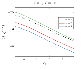
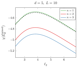
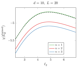
Figure 3: Log-log plot of the Holevo $\chi$-quantity as a function of $b-a=\ell_{2}$ for different values of subsystem size of $A$, $L$, and different $a=d+L$, i.e. different distances between $A$ and $B$. The $\chi$-quantity corresponds to the green line $n=1$ and it has been obtained by using a numerical approach. The black dashed line is the approximation in Eq. (40), valid for $\ell_{2}\gg\epsilon$. As a reference, we also plot different values of $n$ for $\frac{1}{2(1-n)}\log\frac{M_{11}^{n}}{\mathrm{det}M}$.

To have a more refined analysis about the bound on the accessible information we can extract from our charge-projected ensemble, we can evaluate the Holevo $\chi$-quantity, which reads from Eq. (37)

$$\chi(\mathcal{E}^{\rm mixed}_{\mathcal{Q}})\equiv S_{A}^{(1)}(\rho_{A})-\sum_{q}p_{q}S^{(1)}_{A}(\Pi^{B}_{q}|\Psi\rangle)=\lim_{n\to 1}\dfrac{1}{2(1-n)}\log\dfrac{M_{11}^{n}}{\mathrm{det}M}.$$ (38)

However, this would require performing an analytic continuation that we do not know how to evaluate. We can bypass this problem by using a numerical approach [60]. We report the result of this numerical analysis in Fig. 3 by fixing the size of $A$, $L$, the position $a=d+L$ and varying $\ell_{2}$, which denotes the size of the measured region. We observe that as far as $A$ and $B$ are distant, the Holevo-quantity increases for small values of $\ell_{2}$, and then it slowly decreases. This implies that there exists an optimal size of $B$ from which we can ‘maximally’ extract information about $A$, but after this threshold, since the subsystem size of $A$ is fixed, the more we measure $B$, the less information we gain about $A$. In other words, given a set of measurements, $\{q_{i}\}$, the corresponding sequence of states $\{\rho_{A,q_{i}}\}$ becomes too large if the number of measurements (subsystem size of $B$ in this case) is huge compared to the size of $A$, and therefore reconstructing $\rho_{A}$ is even more complicated. On the other hand, if $\ell_{2}$ is small enough and $A$ and $B$ are distant, we can explain the increase in the upper bound of the accessible information by noting that, in the system we are considering, the correlations between $A$ and $B$ decay algebraically, so it means that the farther they are, the larger is the size of $B$ we need to measure to gain information about $A$, at least before the threshold above mentioned.

We also remark here an important difference between our setup and the case of a standard projected ensemble: after our measurement and partial trace over $\overline{A}$, we get an ensemble of mixed states and the bound on the accessible information depends on the size of the subsystem $B$. On the other hand, for the projected ensembles described by Eq. (2), the Holevo $\chi$-quantity reduces to the standard entanglement entropy of $\rho_{A}$, so it does not depend at all on the size of the projected region.

If we focus on the regime $\widetilde{a}_{0}\gg\widetilde{a}_{j}$ in Eq. (30), we can obtain a close expression for the analytical continuation above. Indeed, the second term in Eq. (37) can be rewritten as

$$\begin{split}\frac{\log\det M-n\log M_{11}}{2(n-1)}&=-\frac{1}{2(n-1)}\sum_{k=0}^{n-1}\log[1+\sum_{j=1}^{n-1}e^{2\pi ikj/n}\frac{\widetilde{a}_{j}(n)}{\widetilde{a}_{0}(n)}]+\frac{n}{2(n-1)}\log\frac{\widetilde{a}_{0}(1)}{\widetilde{a}_{0}(n)}\\ &\stackrel{{\scriptstyle\widetilde{a}_{0}\gg\widetilde{a}_{j}}}{{\simeq}}-\frac{1}{2(n-1)}\sum_{k=0}^{n-1}\sum_{j=1}^{n-1}e^{2\pi ikj/n}\frac{\widetilde{a}_{j}(n)}{\widetilde{a}_{0}(n)}+\frac{n}{2(n-1)}\log\frac{\widetilde{a}_{0}(1)}{\widetilde{a}_{0}(n)}.\end{split}$$ (39)

The only non-vanishing contribution of the expression above comes from the second term because the sum over $k$ imposes $j=0$, which is absent, such that

$$\lim_{n\to 1}\frac{1}{2(n-1)}\log\frac{\det M}{M^{n}_{11}}\simeq\frac{1}{\log\left(\frac{b-a}{2\epsilon}\right)}-\frac{(2ab-L(a+b))\log\left[\frac{a(b-L)}{b(a-L)}\right]}{2L(b-a)\log\left(\frac{b-a}{2\epsilon}\right)}.$$ (40)

We report this approximation for the analytical continuation as black dashed lines in Fig. 3. We observe that, as we increase the distance between $A$ and $B$ and $\ell_{2}\gg\epsilon$, the approximation get closer and closer to the exact solution.

We can slightly generalize the result above by considering a dynamical setup, where we measure the charge of the subsystem $B$ at time $t-i\epsilon^{\prime}$. This means that we have to be careful when we consider the anti-holomorphic part. Indeed, the chiral components can be obtained from Eq. (18), by shifting $a,b$ as $a\to a+i(\tau-\epsilon^{\prime})$ and $b\to b+i(\tau-\epsilon^{\prime})$, while for the anti-holomorphic components we should consider $a\to a+i(\tau+\epsilon^{\prime})$ and $b\to b+i(\tau+\epsilon^{\prime})$. Therefore, the matrix $M$ is $2n\times 2n$, it acquires a non-trivial time dependence but preserves its symmetric circulant structure. In the large time limit, we can compute

$$\lim_{n\to 1}\frac{1}{2(n-1)}\log\frac{\det M(t)}{M^{n}_{11}(t)}\stackrel{{\scriptstyle t\to\infty}}{{\simeq}}\frac{(b-a)^{2}L^{2}}{24\log[(b-a)/(2\epsilon)]t^{4}},$$ (41)

which implies that the measurement-induced entanglement in Eq. (37) simply reduces to the total von Neumann entropy between $A$ and $\overline{A}$, $S_{A}^{1}$, and the accessible information goes to 0. In other words, at large time, the effect of the partial measurement of the charge vanishes, as one would have expected.

4 Projecting other operators

In this section, we will consider the situation where we project some other operator, not necessarily the charge. However, we will still assume that it is extensive

$$Q_{B}=\int_{B}dx\ \mathcal{O}(x),$$ (42)

and $\mathcal{O}$ is a Hermitian operator. It can be either a scalar primary $\mathcal{O}_{s}(z,\overline{z})$ of dimension $(h_{s}/2,h_{s}/2)$ or a non-conserving vector $j_{0}(z,\overline{z})$, which is a sum of two operators of weight $(1+h_{v}/2,h_{v}/2)$ and $(h_{v}/2,1+h_{v}/2)$ to make it Hermitian. The real $x$ variable we are using parameterizes the $t=0$ slice, $z=\overline{z}=x$. Finally, we should keep in mind that $h_{s,v}$ cannot be too large, since irrelevant operators in QFT are very UV-sensitive. We will make this statement more precise below.

The steps we need to perform to study the observable-projected ensemble are the same as in the previous section. The reduced density matrix $\rho_{A,q}$ after the projection is defined in exactly the same way (c.f. Eq. (11))

$$\rho_{A,q}=\frac{1}{\mathcal{N}}\int d\gamma\ e^{-i\alpha q}\operatorname*{Tr}_{\overline{A}}(e^{i\gamma Q_{B}}\rho).$$ (43)

In evaluating the Renyi entropies $\operatorname*{Tr}\rho_{A,q}^{n}$, we can again perform a conformal transformation $w(z)$, as in Fig. 2, to map it to a correlation function on a sphere. However, now we have to take into account the Jacobian factors. For example, for a primary operator of dimension $(h_{s}/2,h_{s}/2)$, we need to evaluate

$$\langle\exp\left(i\sum^{n}_{k=1}\gamma_{k}\int_{a}^{b}dx\ \left(\frac{\partial w_{k}}{\partial x}\frac{\partial\overline{w}_{k}}{\partial x}\right)^{h_{s}/2}\mathcal{O}_{s}(w_{k}(x),\overline{w_{k}}(x))\right)\rangle_{\mathbb{C}},$$ (44)

where for convenience we kept the original integration variable $x$ and $w_{k}$ are different branches of the conformal mapping $w(z)$

$$w_{k}=e^{2\pi ik/n}\left(\frac{z}{z-L}\right)^{1/n}.$$ (45)

Without additional assumptions, it would be very hard to evaluate these expectation values. The only general statement we can make is that if $a\rightarrow b$ or $L\rightarrow 0$ we get the operator product expansion (OPE) limit in which the correlations of the measured observables among different replicas decouple and we simply obtain the standard Rényi entropies.

We can derive significant results if we assume that $\mathcal{O}$ has Gaussian correlators. This assumption is not very restrictive since several models satisfy this criterion, such as free theories, holographic theories, and the so-called symmetric orbifold CFTs. The latter are defined as follows: we can take $N$ copies of any “seed" CFT $T$, which we denote as $T^{\otimes n}$ and consider the following quotient:

$$\text{Sym orbifold}(T)=\frac{T^{\otimes N}}{\text{Sym}_{N}}.$$ (46)

An example of an operator in this theory (sometimes called untwisted sector) is

$$\mathcal{O}_{s}=\frac{1}{N}\sum_{i=1}^{N}\mathcal{O}_{i},$$ (47)

where $\mathcal{O}_{i}$ belong to different copies. Thanks to the central limit theorem the correlations of $\mathcal{O}_{s}$ are Gaussian for large $N$.

If $\mathcal{O}$ are Gaussian operators, then we can again use the Wick contractions to arrive at

$$\dfrac{\operatorname*{Tr}\prod_{k=1}^{n}\operatorname*{Tr}_{\overline{A}}[\rho e^{iQ_{B}\gamma_{k}}]}{\operatorname*{Tr}\rho_{A}^{n}}=\exp\left(-\frac{1}{2}\sum_{ij}\gamma_{i}\gamma_{j}M_{ij}\right),$$ (48)

where $M$ depends on the type of operator we are studying.

Beyond the Gaussian fields, we can look at Eq. (48) as a leading perturbative expansion in $\gamma$. In section 6, we will check our predictions against the numerical computations in the Majorana CFT where the charge field is indeed non-Gaussian. Also, we will see in section 5 that such quantities with fixed $\gamma$ (charge distribution generating functions) have better UV properties.

For $\mathcal{O}=\mathcal{O}_{s}(z,\overline{z})$, the matrix elements are given by

$$M_{ij}=\int dx_{1}dx_{2}\langle\mathcal{O}_{s}(w_{i}(x_{1}),\overline{w_{i}}(x_{1}))\mathcal{O}_{s}(w_{j}(x_{2}),\overline{w_{j}}(x_{2}))\rangle\left(\frac{\partial w_{i}}{\partial x_{1}}\frac{\partial\overline{w_{i}}}{\partial x_{1}}\right)^{h_{s}/2}\left(\frac{\partial w_{j}}{\partial x_{2}}\frac{\partial\overline{w_{j}}}{\partial x_{2}}\right)^{h_{s}/2},$$ (49)

while for the vector $j_{0}$:

$$M_{ij}=\int dx_{1}dx_{2}\langle j_{0}(w_{i}(x_{1}),\overline{w_{i}}(x_{1}))j_{0}(w_{j}(x_{2}),\overline{w_{j}}(x_{2}))\rangle\times$$

$$\times\left(\frac{\partial w_{i}}{\partial x_{1}}\right)^{1+h_{v}/2}\left(\frac{\partial\overline{w_{i}}}{\partial x_{1}}\right)^{h_{v}/2}\left(\frac{\partial w_{j}}{\partial x_{2}}\right)^{1+h_{v}/2}\left(\frac{\partial\overline{w_{j}}}{\partial x_{2}}\right)^{h_{v}/2}+h.c.$$

In the $w$ plane, the correlation function of $\mathcal{O}$ can be easily evaluated in the ground state

$$\langle\mathcal{O}_{s}(w_{i},\overline{w_{i}})\mathcal{O}_{s}(w_{j},\overline{w_{j}})\rangle=\frac{1}{|w_{i}-w_{j}|^{2h_{s}}},$$ (50)

$$\langle j_{0}(w_{i},\overline{w_{i}})j_{0}(w_{j},\overline{w_{j}})\rangle=-\frac{1}{(w_{i}-w_{j})^{2}|w_{i}-w_{j}|^{2h_{v}}}.$$ (51)

For simplicity, we have normalized them to $1$, since a global prefactor would only affect the overall “charge" distribution variance. The signs are fixed by requiring reflection-positivity in the Euclidean spacetime. Once we plug these expressions in the matrix elements $M_{ij}$, the resulting integrals can only be evaluated numerically. However, we can still discuss a few general features of these expressions.

Notice that for $n=2$, the complex conjugation in the equations above is not relevant, because $w_{1}=-w_{2}$ are real variables. Hence the answer depends only on the total operator dimension, except for a possible UV-divergent non-universal part - see e.g. Eq. (55).

The integrals (49), (4) are finite for $i\neq j$ because $w_{i}\neq w_{j}$, while for $i=j$, the correlators diverge and the resulting singularity might not be integrable. However, this divergence is universal in the following sense: since it comes from two points colliding, the divergence structure does not depend on the number of replicas or the interval lengths. For example, for the $(h_{s}/2,h_{s}/2)$ case the integrand for $M_{ii}$ has the following form at $x_{1}\approx x_{2}$:

$$\langle\mathcal{O}_{s}(w_{j}(x_{1}),\overline{w_{j}}(x_{1}))\mathcal{O}_{s}(w_{j}(x_{2}),\overline{w_{j}}(x_{2}))\rangle\left(\frac{\partial w_{j}}{\partial x_{1}}\frac{\partial\overline{w_{j}}}{\partial x_{1}}\right)^{h_{s}/2}\left(\frac{\partial w_{j}}{\partial x_{2}}\frac{\partial\overline{w_{j}}}{\partial x_{2}}\right)^{h_{s}/2}\approx$$

$$\approx\frac{1}{(x_{1}-x_{2})^{2h_{s}}}\left(1+\frac{h_{s}L(n^{2}-1)(x_{1}-x_{2})^{2}}{12n^{2}(L-x_{2})^{2}x_{2}^{2}}+\dots\right).$$

Hence, if the operator is not too irrelevant, that is $h_{s}<3/2$, we can remove the divergence by subtracting $1/(x_{1}-x_{2})^{2h_{s}}$, which is simply the two-point function of $\mathcal{O}_{s}(x)$ on a plane. Correspondingly, the integral of $1/(x_{1}-x_{2})^{2h_{s}}$ controls the distribution of $Q_{B}$ for a single interval. The same conclusion holds for the vector case if we impose $h_{v}<1/2$. We will return to this observation later when we discuss how to define UV-finite quantities, while now we evaluate the entanglement entropy. We also notice that, if $h_{s}<1/2$, then UV divergences completely disappear.

Similar to the charge case, we can integrate over $\gamma_{k}$ with the weight $\exp(-iq\sum_{k}\gamma_{k})$ and we get

$$\frac{\operatorname*{Tr}\rho_{A,q}^{n}}{\mathrm{Tr}\rho_{A}^{n}}=\frac{e^{-q^{2}C_{n}/2}}{\sqrt{\det M}}\left(\frac{e^{-q^{2}C_{1}/2}}{\sqrt{M_{11}}}\right)^{-n},$$ (52)

where $C_{n}=(1,\dots)^{T}M^{-1}(1,\dots)$. Subtracting the UV-divergent terms at this stage would be very difficult because $C_{n}$ is highly non-linear in $M$.

Unlike the case in which the observable is simply the charge operator of a compact boson, (see Eq. (33)), we could not find an explicit formula for $C_{n}$. However, it is relatively easy to find it numerically. Two important features, which are not present in the charge case (33), are:

• $C_{n}$ is not linear in $n$ - Fig. 4 (left panel).

• $C_{n}$ depends on the length $L$ of the interval $A$ (the one for which we evaluate the entanglement entropy) - Fig. 4 (right panel).

Moreover, we have numerically checked that $C_{n}$ is not even a function of the conformal cross-ratio of the two intervals $A$ and $B$.

If we sum over all the possible measurement outcomes $q$, we get

$${\rm MIE}(A:\overline{A\cup B})\simeq S_{A}^{(n)}+\dfrac{1}{2(1-n)}\log\dfrac{M_{11}^{n}}{\mathrm{det}M}-\frac{C_{n}-nC_{1}}{2\sqrt{2\pi C_{1}^{3}M_{11}}(1-n)},$$ (53)

where we have used that $\sum_{q}p_{q}q^{2}\simeq(2\pi C_{1}^{3}M_{11})^{-1/2}$. Contrarily to the result (37), the equation above displays a non-trivial dependence on the size of $A$ and on the measured region through the last term.

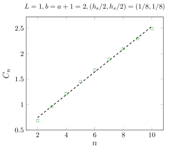
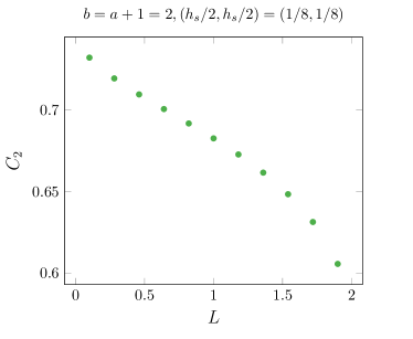
Figure 4: Plot of the $C_{n}$ coefficient defined in Eq. (52). In the left panel, we prove that its dependence on $n$ is nonlinear, as the disagreement between the exact numerical values of $C_{n}$ (symbols) and the best linear fit (dashed black line) shows. In the right panel, we plot the non-trivial $L$ dependence of $C_{2}$ for the 2-replica computation. In both cases, we have used the operator with conformal weight $(1/8,1/8)$.

It is important to discuss the relevant point-splitting procedure for the evaluation of the integrals (49), (4). The main point is that it has to preserve the current conservation (e.g. $\partial_{\overline{z}}j_{0}(z)=0$), which means that the regularization must not mix holomorphic and anti-holomorphic parts. For example, the integrand for the two-point function of a conserved current appearing in Eq. (24) must be regularized as

$$\int dz_{1}dz_{2}\ \frac{1}{(z_{1}-z_{2})^{2}}\rightarrow\int dz_{1}dz_{2}\ \frac{1}{(z_{1}-z_{2}+i\epsilon)^{2}}.$$ (54)

Alternatively, one can understand it as adding an extra $i\epsilon$ Euclidean time evolution before the operators are inserted.

Now, for the scalar operator of dimension $(h_{s}/2,h_{s}/2)$ the integral after regularization becomes

$$\int_{a}^{b}\frac{dz_{1}dz_{2}}{|z_{1}-z_{2}|^{2h_{s}}}\rightarrow\int_{a}^{b}\frac{dz_{1}dz_{2}}{(|z_{1}-z_{2}|^{2}+\epsilon^{2})^{h_{s}}}=\frac{1}{-1+2h_{s}}|b-a|\epsilon^{1-2h_{s}}+\frac{|b-a|^{2-2h_{s}}}{1-3h_{s}+2h_{s}^{2}}+\mathcal{O}(\epsilon).$$ (55)

Some special cases are $h_{s}=1/2$

$$\int_{a}^{b}\frac{dz_{1}dz_{2}}{|z_{1}-z_{2}+i\epsilon|}=2(b-a)\left(\log\frac{|b-a|}{\epsilon}-1\right),$$ (56)

and $h_{s}=1$

$$\int_{a}^{b}\frac{dz_{1}dz_{2}}{|z_{1}-z_{2}+i\epsilon|^{2}}=\frac{\pi|b-a|}{\epsilon}-2\left(1+\log\frac{|b-a|}{\epsilon}\right)+\mathcal{O}(\epsilon).$$ (57)

For the vector case, we have the following regularized integral:

$$\int_{a}^{b}dz_{1}dz_{2}\frac{-1}{(z_{1}-z_{2}+i\epsilon)^{2}(|z_{1}-z_{2}|^{2}+\epsilon^{2})^{h_{v}}},$$ (58)

which is much harder to evaluate. For small $\epsilon$, it yields a series of terms starting with $\epsilon^{-1-2h_{v}}$ with non-universal coefficients plus a regular term $|b-a|^{-2h_{v}}$ with a universal coefficient. One can adopt a slightly different regularization where this universal term can be easily evaluated for $h_{v}>0$:

$$\int_{a}^{b}dz_{1}dz_{2}\frac{-1}{(z_{1}-z_{2}+i\epsilon)^{2}|z_{1}-z_{2}|^{2h_{v}}}=-\frac{\operatorname{const}}{\epsilon^{2h_{v}}}+\dots+\frac{|b-a|^{2h_{v}}}{2h_{v}(1+2h_{v})}+\mathcal{O}(\epsilon).$$ (59)

5 Extracting universal quantities

In the previous sections, we showed that computing the entropy after the projections produces UV divergences if we measure an operator of large conformal dimensions. These divergences, however, are tied to colliding operators and are replica-diagonal. Thus it seems possible to subtract them in a physical way. In this section, we discuss how to do it by studying quantities related to an observable-projected ensemble.

The probabilities $p_{q}$ of observing different charges, or more generally extensive quantities $\int_{B}dx\ \mathcal{O}$ inside the region $B$, are determined by the Born rule

$$p_{q}=\operatorname*{Tr}(\Pi_{q}\rho).$$ (60)

Summing over $q$ with $e^{i\gamma q}$ weight produces the generating function $\langle e^{i\gamma Q_{B}}\rangle$,

$$\sum_{q}p_{q}e^{i\gamma q}=\operatorname*{Tr}(\rho e^{i\gamma Q_{B}}).$$ (61)

By preparing two copies of the system and measuring $q_{1},q_{2}$ inside the two copies of $B$, we can access the overlap (for example, by performing a swap test)

$$R_{q_{1}q_{2}}=\operatorname*{Tr}(\rho_{A,q_{1}}\rho_{A,q_{2}}),$$ (62)

where the post-measurement state of $A$ is

$$\rho_{A,q}=\frac{1}{p_{q}}\operatorname*{Tr}_{\overline{A}}(\Pi_{q}\rho\Pi_{q})\equiv\frac{1}{p_{q}}\widetilde{\rho}_{A,q},$$ (63)

with $\widetilde{\rho}_{A,q}$ the unnormalized density matrix

$$\widetilde{\rho}_{A,q}=\frac{1}{(2\pi)^{2}}\operatorname*{Tr}_{\overline{A}}\int d\gamma_{1}d\gamma_{2}\ e^{i\gamma_{1}q-i\gamma_{2}q}e^{-i\gamma_{1}Q_{B}}\rho e^{+i\gamma_{2}Q_{B}}.$$ (64)

We remark that Eq. (62) represents the distance between two operators, $\rho_{A,q_{1}}$ and $\rho_{A,q_{2}}$, so measuring $R_{q_{1}q_{2}}$ can be relevant to understand how much two operators are distinguishable if $q_{1}\neq q_{2}$. Since $B\in\overline{A}$, we can move $e^{i\gamma_{i}Q_{B}}$ inside the trace in Eq. (64) to obtain

$$\widetilde{\rho}_{A,q}=\frac{1}{2\pi}\operatorname*{Tr}_{\overline{A}}\int d\gamma\ e^{-i\gamma q}\rho e^{i\gamma Q_{B}}\equiv\frac{1}{2\pi}\int d\gamma\ e^{-i\gamma q}\widetilde{\rho}_{A,\gamma}.$$ (65)

Therefore, if we prepare the system samples and compute the average $R_{q_{1}q_{2}}$ over the charges with weights $e^{i\gamma_{1}q_{1}+i\gamma_{2}q_{2}}$, it will yield

$$\sum_{q_{1}q_{2}}e^{i\gamma_{1}q_{1}+i\gamma_{2}q_{2}}p_{q_{1}}p_{q_{2}}R_{q_{1}q_{2}}=\sum_{q_{1}q_{2}}e^{i\gamma_{1}q_{1}+i\gamma_{2}q_{2}}\operatorname*{Tr}_{A}\left(\widetilde{\rho}_{A,q_{1}}\widetilde{\rho}_{A,q_{2}}\right)=$$ (66)

$$=\frac{1}{(2\pi)^{2}}\sum_{q_{1}q_{2}}e^{i\gamma_{1}q_{1}+i\gamma_{2}q_{2}}\int d\gamma_{1}d\gamma_{2}e^{-iq_{1}\gamma_{1}-iq_{2}\gamma_{2}}\operatorname*{Tr}_{A}(\widetilde{\rho}_{A,\gamma_{1}}\widetilde{\rho}_{A,\gamma_{2}}).$$ (67)

By explicitly summing over $q_{1},q_{2}$, Eq. (66) gives

$$\sum_{q_{1}q_{2}}e^{i\gamma_{1}q_{1}+i\gamma_{2}q_{2}}p_{q_{1}}p_{q_{2}}R_{q_{1}q_{2}}=\operatorname*{Tr}(\widetilde{\rho}_{A,\gamma_{1}}\widetilde{\rho}_{A,\gamma_{2}}),$$ (68)

which is a two-replica calculation with the appropriate fluxes. As we discussed before, the UV divergences arise only within each replica copy and they are the same as in computing $\langle e^{i\gamma_{1}Q_{B}}\rangle$. Even though, strictly speaking, our arguments are based on an explicit Gaussian computation, in Sec. 5.1, we will argue that they hold more generally. Hence, if we divide Eq. (68) by $\langle e^{i\gamma_{1}Q_{B}}\rangle\langle e^{i\gamma_{2}Q_{B}}\rangle$, the UV-divergence will cancel and

$$\frac{\operatorname*{Tr}(\widetilde{\rho}_{A,\gamma_{1}}\widetilde{\rho}_{A,\gamma_{2}})}{\langle e^{i\gamma_{1}Q_{B}}\rangle\langle e^{i\gamma_{2}Q_{B}}\rangle}\ -\ \text{UV-finite}.$$ (69)

The above observable is unusual because it includes the overlap of two different states and it might be difficult to access it theoretically or experimentally.

A more standard object to study is the averaged purity:

$$\sum_{q}p_{q}e^{i\gamma q}\operatorname*{Tr}(\rho_{A,q}^{2})=\sum_{q}\int d\gamma_{1}d\gamma_{2}e^{i\gamma q-i\gamma_{1}q-i\gamma_{2}q}\operatorname*{Tr}(\rho_{A,\gamma_{1}}\rho_{A,\gamma_{2}}).$$ (70)

Let us repeat the analysis above to see if it can be made finite by dividing by a correlation function involving $e^{iQ_{B}}$. Now the sum over $q$ projects $\gamma_{1}+\gamma_{2}=\gamma$, so we need to compute the integral

$$\int d\gamma_{1}d\gamma_{2}\ \delta(\gamma-\gamma_{1}-\gamma_{2})e^{-M_{11}\gamma_{1}^{2}/2-\gamma_{1}\gamma_{2}M_{12}-M_{22}\gamma_{2}^{2}/2}.$$ (71)

After simple manipulations, it leads to

$$\sum_{q}p_{q}e^{i\gamma q}\operatorname*{Tr}(\rho_{A,q}^{2})=\frac{\sqrt{\pi}}{\sqrt{M_{11}-M_{12}}}\exp\left(-\frac{\gamma^{2}}{4}(M_{11}-M_{12})\right).$$ (72)

Hence we can still find a UV-finite quantity if we divide Eq. (72) by $\langle e^{i\gamma Q_{B}/\sqrt{2}}\rangle$.

5.1 Introducing interactions

In the previous part, we explained that the ratio

$$\frac{\operatorname*{Tr}(\widetilde{\rho}_{A,\gamma_{1}}\widetilde{\rho}_{A,\gamma_{2}})}{\langle e^{i\gamma_{1}Q_{B}}\rangle\langle e^{i\gamma_{2}Q_{B}}\rangle}$$ (73)

is UV-finite and our arguments were based on the explicit expression for Gaussian theories found in Sec. 4. Now, we would like to argue that it is true more generally. The idea is that interactions introduce extra smearing, so the diagrams are less divergent. In other words, diagrams that involve interactions are finite. We can illustrate this by evaluating the expectation value $\langle e^{i\gamma Q_{B}}\rangle$. Let us imagine that we are drawing all possible Feynman diagrams associated with this quantity. As usual, disconnected diagrams combine into an exponent of connected ones [61], so we only need to focus on connected diagrams. A generic connected diagram is illustrated in Fig. 5. Importantly, we will assume that the interaction vertex $V(z,\overline{z})$ can be connected to $k$ copies of $Q$ and that it has no extra derivatives, so the external propagators are simply the $\mathcal{O}_{s}$ Green functions. The analysis below can be easily modified to include these possibilities.

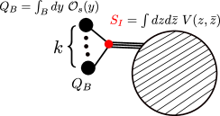
Figure 5: A generic diagram contributing to $\langle e^{i\gamma Q_{B}}\rangle$.

As in the rest of the paper we can consider two cases: measuring a scalar operator of the conformal weight $(h_{s}/2,h_{s}/2)$ or a vector with weights $(1+h_{v}/2,h_{v}/2)$ and $(h_{v}/2,1+h_{v}/2)$.

We can start from the scalar case, where the external propagator is

$$\int_{B=[a,b]}dy\ \frac{1}{((y-z)(y-\overline{z}))^{h_{s}}},$$ (74)

and $z,\overline{z}$ are the coordinates of the interaction vertex represented by the red blob. If we assume that $z$ is outside the interval $B$, the integral over $y$ can be computed exactly and it gives

$$-(-1)^{h_{s}}\frac{1}{1-h_{s}}(y-\overline{z})^{1-h_{s}}\left(\frac{1}{z-\overline{z}}\right)^{h_{s}}\phantom{m}_{2}F_{1}\left(1-h_{s},h_{s},2-h_{s},\frac{y-\overline{z}}{z-\overline{z}}\right)\Big{|}^{y=b}_{y=a}.$$ (75)

Since there might be several $Q_{B}$ insertions leading to the same vertex, Eq. (75) must be taken to some power $k$. The second step is to perform the integral over $z,\overline{z}$, which is more complicated. Indeed, it might have additional UV divergences coming from points colliding inside the blob (which can be canceled by adding counter-terms), and also when $z,\overline{z}$ are inside the interval $B$ or near its endpoints. For small $z-\overline{z}$ the hypergeometric function in Eq. (75) has the following expansion

$$\phantom{m}{}_{2}F_{1}\left(1-h_{s},h_{s},2-h_{s},\frac{y-\overline{z}}{z-\overline{z}}\right)=\\ -e^{\pm i\pi h_{s}}\frac{\Gamma(2-h_{s})\Gamma(-1+2h_{s})}{\Gamma(h_{s})}\left(\frac{y-\overline{z}}{z-\overline{z}}\right)^{h_{s}-1}+\mathcal{O}((z-\overline{z})^{h_{s}}).$$ (76)

After plugging it in Eq. (75), we notice that the factor $(y-\overline{z})^{1-h_{s}}$ cancels up to a possible phase. This phase is determined by the prefactor $e^{\pm i\pi h}$ which comes from the hypergeometric function branch cut. If $z$ is real and outside the interval $[a,b]$ then the points $y=a$ and $y=b$ come with the same phase and the divergence $(z-\overline{z})^{1-h_{s}}$ cancels out. However, if $z$ is between $a$ and $b$ then the phase $e^{\pm i\pi h_{s}}$ is different and the integrand blows up as

$$\left(\frac{1}{(z-\overline{z})^{2h_{s}-1}}\right)^{k},$$ (77)

if $h_{s}>1/2$, otherwise it is finite. Does this behavior lead to a divergent integral? It is natural to assume that the interaction vertex $V(z,\overline{z})$ has conformal dimension less than $2$, but it contains at least $k$ insertions of $\mathcal{O}_{h_{s}/2,h_{s}/2}$, hence

$$kh_{s}<2.$$ (78)

At the same time $k\geq 1$. Therefore, we can conclude that the negative power of $(z-\overline{z})$ in the integrand is

$$k(2h_{s}-1)=2kh_{s}-k\leq 4-1=3.$$ (79)

So, in principle, the integral in $z,\overline{z}$ can still be divergent and to ensure its convergence we need to impose

$$2kh_{s}-k\leq 1\rightarrow h_{s}\leq\cfrac{1}{2}+\frac{1}{2k}.$$ (80)

If this condition is satisfied, the divergent contributions only arise from the free-field behavior, hence the ratio (73) will be finite. We should emphasize that $k$ here is not a fixed number, but it represents how many operators $\mathcal{O}_{s}$ could couple to the interaction vertex. For example, for a scalar field $\phi$, if $\mathcal{O}_{s}=\phi$ and $V=\phi^{4}$, then $k$ can be $1,2,3$ or $4$. The inequality is the strictest for the maximal possible $k$.

The case of a vector operator with weights $(h_{v}/2+1,h_{v}/2)+(h_{v}/2,h_{v}/2+1)$ is similar. Instead of Eq. (74), the integrand is $1/((y-z)^{2}|y-z|^{2h_{v}})$. After integrating over $y$, the resulting expression has the following behavior for small $z-\overline{z}$:

$$\frac{1}{(z-\overline{z})^{2h_{v}}}.$$ (81)

Again, assuming that the interaction vertex has degree $k$, we need to impose the following inequality to ensure that the $z,\overline{z}$ integral is convergent

$$h_{v}\leq\frac{1}{2k}.$$ (82)

To summarize, we have shown that by using observable-projected ensembles, it is possible to extract UV-finite quantities also in the presence of interactions generated by operators with low scaling dimension.

6 Numerical Checks

In the sections above we have shown it is possible to compute the entanglement properties of the observable-projected ensembles in field theory. Now, we show how it is possible to address this question also numerically, when the observable we measure is the charge. We focus on the ground state of the Hamiltonian

$$H=-\frac{1}{2}\sum_{j=-\infty}^{\infty}\left(c^{\dagger}_{j}c_{j+1}+\kappa c^{\dagger}_{j}c^{\dagger}_{j+1}+\mathrm{h.c.}+2hc^{\dagger}_{j}c_{j}\right),$$ (83)

for two sets of parameters: when $\kappa=h=1$, it reduces to a critical Majorana chain, while for $\kappa=h=0$ is corresponds to a tight-binding model with $U(1)$ symmetry (whose continuum limit is described in section 3 for $K=1$). Here $\boldsymbol{c}_{j}=(c_{j}^{\dagger},c_{j})$ are the fermionic operators. We consider an infinite system $A\cup B\cup C$ and we define $\rho_{AB}=\mathrm{Tr}(\rho_{ABC})$ (i.e. $\overline{A}=B\cup C$). The reduced density matrix $\rho_{AB}$ of the ground state of the Hamiltonian (83) is a Gaussian operator in terms of $\boldsymbol{c}_{j}$ [62]. Therefore, we can express our quantities of interest in terms of the two-point correlation matrix

$$\Gamma_{jj^{\prime}}=2\mathrm{Tr}\left[\rho_{A}\boldsymbol{c}_{j}^{\dagger}\boldsymbol{c}_{j^{\prime}}\right]-\delta_{jj^{\prime}},$$ (84)

with $j,j^{\prime}\in AB$. Since $\rho_{AB}$ is a Gaussian operator, we can write it as

$$\mathrm{Tr}_{B}(\rho_{AB}e^{i\gamma Q_{B}})=\mathrm{Tr}_{B}\left(\frac{1}{Z_{AB}}e^{-\sum_{jj^{\prime}}\boldsymbol{c}_{j}^{\dagger}h_{jj^{\prime}}\boldsymbol{c}_{j^{\prime}}}e^{i\gamma\sum_{jj^{\prime}}\boldsymbol{c}_{j}^{\dagger}n^{B}_{jj^{\prime}}\boldsymbol{c}_{j^{\prime}}}\right),$$ (85)

where $n^{B}_{jj^{\prime}}=0$ if $j,j^{\prime}\in A$ and $n^{B}_{jj^{\prime}}=\sigma^{z}\delta_{jj^{\prime}}$ otherwise, and $Z_{AB}$ is a normalization factor. The operator above involves the product of Gaussian operators, so it is still a Gaussian operator and by using the Baker-Campbell-Haussdorf formula, we can find [63, 57]

$$e^{\sum_{j,j^{\prime}}\boldsymbol{c}_{j}^{\dagger}A_{jj^{\prime}}\boldsymbol{c}_{j^{\prime}}}e^{\sum_{j,j^{\prime}}\boldsymbol{c}_{j}^{\dagger}B_{jj^{\prime}}\boldsymbol{c}_{j^{\prime}}}=e^{\sum_{j,j^{\prime}}\boldsymbol{c}_{j}^{\dagger}H_{jj^{\prime}}\boldsymbol{c}_{j^{\prime}}}$$ (86)

where $H=\log(e^{A}e^{B})$. Therefore, Eq. (85) can be written as

$$\mathrm{Tr}_{B}\left(\frac{1}{Z_{AB}}e^{-\sum_{jj^{\prime}}\boldsymbol{c}_{j}^{\dagger}h^{\gamma}_{jj^{\prime}}\boldsymbol{c}_{j^{\prime}}}\right),\qquad h^{\gamma}=\log(e^{-h}e^{i\gamma n^{B}}).$$ (87)

Moreover, the single-particle entanglement Hamiltonian $h$ of Eq. (85) can be expressed in terms of the correlation matrix (84) as

$$e^{-h}=\frac{1-\Gamma}{1+\Gamma}.$$ (88)

We can now define a normalized operator with trace 1

$$\mathrm{Tr}_{B}\left(\frac{1}{Z^{\gamma}_{AB}}e^{-\sum_{jj^{\prime}}\boldsymbol{c}_{j}^{\dagger}h^{\gamma}_{jj^{\prime}}\boldsymbol{c}_{j^{\prime}}}\right),\qquad Z^{\gamma}_{AB}=\mathrm{Tr}\left(e^{-\sum_{jj^{\prime}}\boldsymbol{c}_{j}^{\dagger}h^{\gamma}_{jj^{\prime}}\boldsymbol{c}_{j^{\prime}}}\right),$$ (89)

and rewrite it as

$$\mathrm{Tr}_{B}\left(\frac{1}{Z^{\alpha}_{AB}}e^{-\sum_{jj^{\prime}}\boldsymbol{c}_{j}^{\dagger}h^{\gamma}_{jj^{\prime}}\boldsymbol{c}_{j^{\prime}}}\right)=\frac{1}{Z^{\gamma}_{A}}e^{-\sum_{jj^{\prime}}\boldsymbol{c}_{j}^{\dagger}h^{\gamma,A}_{jj^{\prime}}\boldsymbol{c}_{j^{\prime}}},\qquad Z^{\gamma}_{A}=\mathrm{Tr}\left(e^{-\sum_{jj^{\prime}}\boldsymbol{c}_{j}^{\dagger}h^{\gamma,A}_{jj^{\prime}}\boldsymbol{c}_{j^{\prime}}}\right),$$ (90)

with

$$e^{-h^{\gamma}}=\frac{1-\Gamma^{\gamma}}{1+\Gamma^{\gamma}}.$$ (91)

For a general non-Hermitian matrix $H$, we can use that [63]

$$\mathrm{Tr}(e^{\sum_{j,j^{\prime}}\boldsymbol{c}_{j}^{\dagger}H_{jj^{\prime}}\boldsymbol{c}_{j}})=\sqrt{\mathrm{det}(1+e^{H})},$$ (92)

and hence

$$Z^{\alpha}_{AB}=\det\left(1+\frac{1-\Gamma}{1+\Gamma}e^{i\gamma n_{B}}\right),\qquad Z^{\alpha}_{A}=\det\left(1+\frac{1-\Gamma^{\gamma}_{A}}{1+\Gamma^{\gamma}_{A}}\right).$$ (93)

We remark that $\Gamma^{\gamma}_{A}$ can be obtained by restricting $\Gamma^{\gamma}$ to the subsystem $A$. If we put everything together, we find that

$$\mathrm{Tr}_{B}\left(\frac{1}{Z_{AB}}e^{-\sum_{jj^{\prime}}\boldsymbol{c}_{j}^{\dagger}h_{jj^{\prime}}\boldsymbol{c}_{j^{\prime}}}e^{i\gamma\sum_{jj^{\prime}}\boldsymbol{c}_{j}^{\dagger}n^{B}_{jj^{\prime}}\boldsymbol{c}_{j^{\prime}}}\right)=\frac{Z_{AB}^{\gamma}}{Z_{AB}}\frac{1}{Z_{A}^{\gamma}}e^{-\sum_{jj^{\prime}}\boldsymbol{c}_{j}^{\dagger}h^{\gamma,A}_{jj^{\prime}}\boldsymbol{c}_{j^{\prime}}},$$ (94)

and for a generic Rényi index $n$

$$\mathrm{Tr}_{A}\left[\prod_{j=1}^{n}\left(\frac{1}{Z_{AB}}e^{-\sum_{jj^{\prime}}\boldsymbol{c}_{j}^{\dagger}h_{jj^{\prime}}\boldsymbol{c}_{j^{\prime}}}e^{i\gamma_{j}\sum_{jj^{\prime}}\boldsymbol{c}_{j}^{\dagger}n^{B}_{jj^{\prime}}\boldsymbol{c}_{j^{\prime}}}\right)\right]=\frac{1}{Z_{AB}^{n}}\prod_{j=1}^{n}\left[\frac{Z_{AB}^{\gamma_{j}}}{Z_{A}^{\gamma_{j}}}\right]\det\left(1+\prod_{j=1}^{n}\frac{1-\Gamma^{\gamma_{j}}_{A}}{1+\Gamma^{\gamma_{j}}_{A}}\right).$$ (95)

If we denote by

$$\frac{Z_{n}(\gamma_{1},\dots,\gamma_{n})}{Z_{n}}=\frac{\mathrm{Tr}_{A}[\prod_{j=1}^{n}\mathrm{Tr}_{B}(\rho_{AB}e^{i\gamma_{j}Q_{B}})]}{\mathrm{Tr}(\rho_{A}^{n})},$$ (96)

we can cross-check the result in Eq. (23) by choosing $\kappa=h=0$ in Eq. (83). We report the comparison between the exact numerical results and our analytical predictions in Fig. 6 for fixed subsystem size $L$, $a=L+d$, and by varying $b-a\equiv\ell_{2}$.

We repeat the same analysis for the ground state of the Majorana chain at its critical point by setting $\kappa=h=1$ in Eq. (83). Despite the lattice operator is quadratic, $Q=\sum_{j}c^{\dagger}_{j}c_{j}$, as well as its continuum counterpart (one of the primary fields of the Ising CFT with scaling dimension $1$), it does not satisfy Wick’s theorem. Therefore, we can use our result (57) only as a perturbative expansion in $\gamma$. From Eq. (57) we expect the presence of a linear term in $\ell_{2}$, whose prefactor $1/\epsilon$ is non-universal, and a subleading logarithmic growth. To find the exact result in all orders in $\gamma$, we should map Eq. (96) to a cylinder with $n$ defects, rather than to the complex plane, as we did in Eq. (45). After the mapping, Ref. [64] proved that this quantity can be related to the ground state energy of the massless Majorana fermion theory on a circle with marginal point defects, at least in the limit in which $a\to 0,b\to L$, i.e. $A$ and $B$ coincide. Our case is slightly different because the boundary conditions that the fields obey along $B$ on the Riemann surface appearing in Fig. 2 are simpler, so each $i$-th sheet can be related to the massless Majorana fermion theory with only one single defect, that in our original problem would be $e^{i\gamma_{i}Q_{B}}$. We can borrow the results from Ref. [64] and we find that our results match up to rescaling $\gamma_{i}\to\textrm{arctanh}(\tan(\gamma_{i}/2))$ in Eq. (48). We cross-check this with the exact numerical results in Fig. 7 focusing on the universal logarithmic term, and we remark that for small values of $\gamma_{i}$, $\textrm{arctanh}(\tan(\gamma_{i}/2))\simeq\gamma_{i}/2$ and our quadratic approximation is valid, as we would expect (dashed black lines). In the large $\ell_{2}$-limit, we stress that this approximation is enough to get the result in Eq. (52).

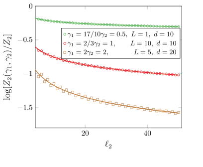
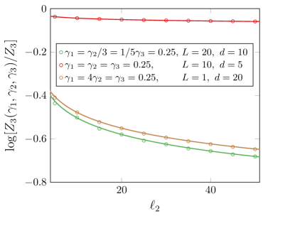
Figure 6: Normalized (logarithm of the) charged moments defined in Eq. (96) as a function of $\ell_{2}$ for different values of $\gamma_{1},\gamma_{2},d,\ell_{1}$. Here we are considering the ground state of the Hamiltonian (83) with $\kappa=h=0$. The curves correspond to our result (23) with an additive constant obtained from a fit, while the symbols are the exact numerical values from Eq. (95). We report only the real part, the imaginary part is due to how the charge is discretized on the lattice.

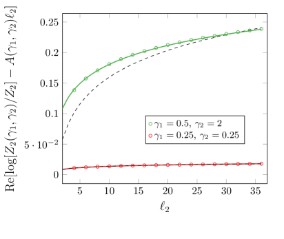
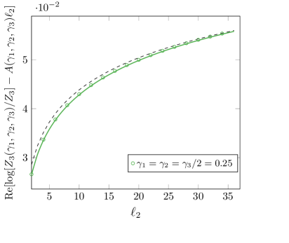
Figure 7: Real part of the normalized (logarithm of the) charged moments defined in Eq. (96) as a function of $\ell_{2}$ for different values of $\gamma$, $\ell_{1}=d=10$ for the ground state of the Majorana chain at the critical point. Once we subtract the non-universal contribution (which is linear in $\ell_{2}$ and we denote it by $A(\gamma_{i})\ell_{2}$), the solid curves have been obtained by plugging Eq. (57) in (48) with $\gamma_{i}\to\frac{1}{\pi}\textrm{arctanh}(\tan(\gamma_{i}/2))$ and an additive fitted constant. The symbols are the exact numerical values from Eq. (95). The black dashed lines correspond to the quadratic approximation in $\gamma_{i}$.

7 Conclusions

In this manuscript, we have investigated the projected ensembles from a novel perspective, considering set of states generated not by partial projective measurements on the system but by measurements of a given observable, like the number of particles or the magnetization. After this operation, we have considered an ensemble of mixed-states and we have investigated the entanglement properties, both for any individual outcome and the measurement-induced entanglement (cf. Eq. (7)). The advantages of considering an observable-projected ensemble are two-fold: as we have shown in the main text, it is amenable to an analytical solution, but at the same time these properties can also be experimentally probed, by using classical shadows and randomized measurements. For a free compact boson, we could compute explicit analytical expressions that have also provided an upper bound on the amount of the information that one can extract about the subsystem $A$ after the measurement of the charge in a non-complementary region, in particular how this is related to the size of the measured system. For generic Gaussian theories, similar computations can be performed, even though the dependence on the geometry becomes more involved. Finally, we suggest how our observable-projected ensemble can be used to extract universal quantities, by properly regularizing UV divergences.

There are several future directions that our manuscript might open. For usual projected ensembles, after averaging the $k$-moments, i.e. constructing $\mathcal{E}_{k}=\mathbb{E}_{\mathcal{E}}\left(|\Psi_{i}\rangle\langle\Psi_{i}|\right)^{\otimes k},$ one can show that, in the absence of symmetries and conservation laws, ergodic systems produce subsystems in the maximally mixed states [30, 31]. We have already mentioned in the introduction that these moments are close to an ensemble of Haar-random states. We can ask a similar question for observable-projected ensembles: after preparing a given state, $\rho$, and letting it evolve with Haar random dynamics, we can construct the ensemble (6) and ask whether the corresponding $k$-moments are close to some universal distribution and they also satisfy a maximum entropy principle [39]. To address this question we can also start from an easier setup in which $A$ and $B$ are complementary systems, we fix the subsystem size of $A$ and we scale the subsystem size of $B$. In general, it would be interesting to study the observable-projected ensemble in a dynamical setup and investigate if phenomena like deep thermalization also occur in this case.

In section 2 we have outlined an experimental proposal to probe the properties of the charge-projected ensembles. This can be doable, for instance, by exploiting the preparation of the ground state of the XXZ spin chain (recently discussed in [65]), which is a microscopic realization of the compact boson studied in section 3.

Our work provides a strategy to study projected ensembles in a field theory setup, by implementing them through local operators depending on the measured observable. On the way to study also the projected ensembles (2) in field theory, Ref. [66] points out that performing a Bell measurement amounts to inserting a boundary changing operator between the measured and the unmeasured part. This implies that if the boundary condition is conformal invariant, the measurement-induced entanglement might reduce to a correlation function of boundary changing operators. A thorough analysis in this direction might allow for studying the projected ensembles in conformal field theories.

Finally, it would be interesting to use observable-projected ensembles to extract information about the initial wavefunction. For instance, in [46], the authors found that measuring stabilizer sign-free states in the sign-free basis cannot generate more correlations than those that already exist, by providing some bounds on the MIE for different systems. On the other hand, these bounds are violated for generic (non-stabilizer) states, for example, critical states with sign structure.

References

- [1] Nathanan Tantivasadakarn, Ryan Thorngren, Ashvin Vishwanath, and Ruben Verresen. “Long-range entanglement from measuring symmetry-protected topological phases”. Phys. Rev. X 14, 021040 (2024).
- [2] Tsung-Cheng Lu, Leonardo A. Lessa, Isaac H. Kim, and Timothy H. Hsieh. “Measurement as a shortcut to long-range entangled quantum matter”. PRX Quantum 3, 040337 (2022).
- [3] Nathanan Tantivasadakarn, Ashvin Vishwanath, and Ruben Verresen. “Hierarchy of topological order from finite-depth unitaries, measurement, and feedforward”. PRX Quantum 4, 020339 (2023).
- [4] Sergey Bravyi, Isaac Kim, Alexander Kliesch, and Robert Koenig. “Adaptive constant-depth circuits for manipulating non-abelian anyons” (2022). arXiv:2205.01933.
- [5] Jong Yeon Lee, Wenjie Ji, Zhen Bi, and Matthew P. A. Fisher. “Decoding measurement-prepared quantum phases and transitions: from ising model to gauge theory, and beyond” (2022). arXiv:2208.11699.
- [6] Guo-Yi Zhu, Nathanan Tantivasadakarn, Ashvin Vishwanath, Simon Trebst, and Ruben Verresen. “Nishimori’s cat: Stable long-range entanglement from finite-depth unitaries and weak measurements”. Phys. Rev. Lett. 131, 200201 (2023).
- [7] Lorenzo Piroli, Georgios Styliaris, and J. Ignacio Cirac. “Quantum circuits assisted by local operations and classical communication: Transformations and phases of matter”. Phys. Rev. Lett. 127, 220503 (2021).
- [8] Yaodong Li, Xiao Chen, and Matthew P. A. Fisher. “Quantum Zeno effect and the many-body entanglement transition”. Phys. Rev. B 98, 205136 (2018).
- [9] Yaodong Li, Xiao Chen, and Matthew P. A. Fisher. “Measurement-driven entanglement transition in hybrid quantum circuits”. Phys. Rev. B 100, 134306 (2019).
- [10] Brian Skinner, Jonathan Ruhman, and Adam Nahum. “Measurement-Induced Phase Transitions in the Dynamics of Entanglement”. Phys. Rev. X 9, 031009 (2019). arXiv:1808.05953.
- [11] Marcin Szyniszewski, Alessandro Romito, and Henning Schomerus. “Entanglement transition from variable-strength weak measurements”. Phys. Rev. B 100, 064204 (2019).
- [12] Marcin Szyniszewski, Alessandro Romito, and Henning Schomerus. “Universality of Entanglement Transitions from Stroboscopic to Continuous Measurements”. Phys. Rev. Lett. 125, 210602 (2020).
- [13] Soonwon Choi, Yimu Bao, Xiao-Liang Qi, and Ehud Altman. “Quantum Error Correction in Scrambling Dynamics and Measurement-Induced Phase Transition”. Phys. Rev. Lett. 125, 030505 (2020). arXiv:1903.05124.
- [14] Sagar Vijay. “Measurement-Driven Phase Transition within a Volume-Law Entangled Phase” (2020). arXiv:2005.03052.
- [15] Yaodong Li and Matthew P. A. Fisher. “Statistical mechanics of quantum error correcting codes”. Physical Review B103 (2021).
- [16] A. Altland, M. Buchhold, S. Diehl, and T. Micklitz. “Dynamics of measured many-body quantum chaotic systems”. Phys. Rev. Res. 4, L022066 (2022). arXiv:2112.08373.
- [17] Alexey Milekhin and Fedor K. Popov. “Measurement-induced phase transition in teleportation and wormholes”. SciPost Phys. 17, 020 (2024). arXiv:2210.03083.
- [18] Beni Yoshida. “Projective measurement of black holes” (2022). arXiv:2203.04968.
- [19] Ruihua Fan, Sagar Vijay, Ashvin Vishwanath, and Yi-Zhuang You. “Self-organized error correction in random unitary circuits with measurement”. Phys. Rev. B 103, 174309 (2021).
- [20] Samuel J. Garratt, Zack Weinstein, and Ehud Altman. “Measurements conspire nonlocally to restructure critical quantum states”. Phys. Rev. X 13, 021026 (2023).
- [21] Samuel J. Garratt and Ehud Altman. “Probing postmeasurement entanglement without postselection”. PRX Quantum 5, 030311 (2024).
- [22] Zack Weinstein, Rohith Sajith, Ehud Altman, and Samuel J. Garratt. “Nonlocality and entanglement in measured critical quantum ising chains”. Phys. Rev. B 107, 245132 (2023).
- [23] Xinyu Sun, Hong Yao, and Shao-Kai Jian. “New critical states induced by measurement” (2023). arXiv:2301.11337.
- [24] Sara Murciano, Pablo Sala, Yue Liu, Roger S. K. Mong, and Jason Alicea. “Measurement-altered ising quantum criticality”. Phys. Rev. X 13, 041042 (2023).
- [25] Alessio Paviglianiti, Xhek Turkeshi, Marco Schirò, and Alessandro Silva. “Enhanced Entanglement in the Measurement-Altered Quantum Ising Chain” (2023). arXiv:2310.02686.
- [26] Rushikesh A. Patil and Andreas W. W. Ludwig. “Highly complex novel critical behavior from the intrinsic randomness of quantum mechanical measurements on critical ground states – a controlled renormalization group analysis” (2024). arXiv:2409.02107.
- [27] Mark Srednicki. “Chaos and quantum thermalization”. Phys. Rev. E 50, 888–901 (1994).
- [28] J. M. Deutsch. “Quantum statistical mechanics in a closed system”. Phys. Rev. A 43, 2046–2049 (1991).
- [29] Pasquale Calabrese and John Cardy. “Entanglement entropy and quantum field theory”. J. Stat. Mech. 2004, P06002 (2004).
- [30] Jordan S. Cotler, Daniel K. Mark, Hsin-Yuan Huang, Felipe Hernández, Joonhee Choi, Adam L. Shaw, Manuel Endres, and Soonwon Choi. “Emergent quantum state designs from individual many-body wave functions”. PRX Quantum 4, 010311 (2023).
- [31] Joonhee Choi, Adam L. Shaw, Ivaylo S. Madjarov, Xin Xie, Ran Finkelstein, Jacob P. Covey, Jordan S. Cotler, Daniel K. Mark, Hsin-Yuan Huang, Anant Kale, Hannes Pichler, Fernando G. S. L. Brandão, Soonwon Choi, and Manuel Endres. “Preparing random states and benchmarking with many-body quantum chaos”. Nature 613, 468–473 (2023).
- [32] Maxime Lucas, Lorenzo Piroli, Jacopo De Nardis, and Andrea De Luca. “Generalized deep thermalization for free fermions”. Phys. Rev. A 107, 032215 (2023).
- [33] Amos Chan and Andrea De Luca. “Projected state ensemble of a generic model of many-body quantum chaos” (2024). arXiv:2402.16939.
- [34] Wen Wei Ho and Soonwon Choi. “Exact emergent quantum state designs from quantum chaotic dynamics”. Phys. Rev. Lett. 128, 060601 (2022).
- [35] Matteo Ippoliti and Wen Wei Ho. “Solvable model of deep thermalization with distinct design times”. Quantum 6, 886 (2022).
- [36] Pieter W. Claeys and Austen Lamacraft. “Emergent quantum state designs and biunitarity in dual-unitary circuit dynamics”. Quantum 6, 738 (2022).
- [37] Matteo Ippoliti and Wen Wei Ho. “Dynamical purification and the emergence of quantum state designs from the projected ensemble”. PRX Quantum 4, 030322 (2023).
- [38] Harshank Shrotriya and Wen Wei Ho. “Nonlocality of deep thermalization” (2023). arXiv:2305.08437.
- [39] Daniel K. Mark, Federica Surace, Andreas Elben, Adam L. Shaw, Joonhee Choi, Gil Refael, Manuel Endres, and Soonwon Choi. “A maximum entropy principle in deep thermalization and in hilbert-space ergodicity” (2024). arXiv:2403.11970.
- [40] Richard Jozsa, Daniel Robb, and William K. Wootters. “Lower bound for accessible information in quantum mechanics”. Phys. Rev. A 49, 668–677 (1994).
- [41] M. A. Rajabpour. “Post-measurement bipartite entanglement entropy in conformal field theories”. Phys. Rev. B 92, 075108 (2015).
- [42] M A Rajabpour. “Entanglement entropy after a partial projective measurement in 1+1 dimensional conformal field theories: exact results”. J. Stat. Mech. 2016, 063109 (2016).
- [43] Jean-Marie Stéphan. “Emptiness formation probability, toeplitz determinants, and conformal field theory”. J. Stat. Mech. 2014, P05010 (2014).
- [44] Jean-Marie Stéphan. “Shannon and rényi mutual information in quantum critical spin chains”. Phys. Rev. B 90, 045424 (2014).
- [45] F. Verstraete, M. Popp, and J. I. Cirac. “Entanglement versus correlations in spin systems”. Phys. Rev. Lett. 92, 027901 (2004).
- [46] Cheng-Ju Lin, Weicheng Ye, Yijian Zou, Shengqi Sang, and Timothy H. Hsieh. “Probing sign structure using measurement-induced entanglement”. Quantum 7, 910 (2023).
- [47] Olalla A. Castro-Alvaredo and Lucía Santamaría-Sanz. “Symmetry resolved measures in quantum field theory: a short review” (2024). arXiv:2403.06652.
- [48] Michael A. Nielsen and Isaac L. Chuang. “Quantum computation and quantum information”. Cambridge University Press. (2000).
- [49] Richard Jozsa, Daniel Robb, and William K. Wootters. “Lower bound for accessible information in quantum mechanics”. Phys. Rev. A 49, 668–677 (1994).
- [50] Alexander. S. Holevo. “The capacity of the quantum channel with general signal states”. IEEE Tran. on Info. Th. 44, 269–273 (1998).
- [51] Andreas Elben, Steven T Flammia, Hsin-Yuan Huang, Richard Kueng, John Preskill, Benoît Vermersch, and Peter Zoller. “The randomized measurement toolbox”. Nat. Rev. Phys. 5, 9–24 (2023).
- [52] Lorenzo Piroli, Georgios Styliaris, and J. Ignacio Cirac. “Approximating many-body quantum states with quantum circuits and measurements” (2024). arXiv:2403.07604.
- [53] Antoine Neven, Jose Carrasco, Vittorio Vitale, Christian Kokail, Andreas Elben, Marcello Dalmonte, Pasquale Calabrese, Peter Zoller, Benoît Vermersch, Richard Kueng, and Barbara Kraus. “Symmetry-resolved entanglement detection using partial transpose moments”. npj Quantum Inf. 7, 152 (2021).
- [54] Vittorio Vitale, Andreas Elben, Richard Kueng, Antoine Neven, Jose Carrasco, Barbara Kraus, Peter Zoller, Pasquale Calabrese, Benoît Vermersch, and Marcello Dalmonte. “Symmetry-resolved dynamical purification in synthetic quantum matter”. SciPost Phys. 12, 1–37 (2022).
- [55] Aniket Rath, Vittorio Vitale, Sara Murciano, Matteo Votto, Jérôme Dubail, Richard Kueng, Cyril Branciard, Pasquale Calabrese, and Benoît Vermersch. “Entanglement barrier and its symmetry resolution: Theory and experimental observation”. PRX Quantum 4, 010318 (2023).
- [56] Lata Kh. Joshi, Johannes Franke, Aniket Rath, Filiberto Ares, Sara Murciano, Florian Kranzl, Rainer Blatt, Peter Zoller, Benoît Vermersch, Pasquale Calabrese, Christian F. Roos, and Manoj K. Joshi. “Observing the quantum mpemba effect in quantum simulations”. Phys. Rev. Lett. 133, 010402 (2024).
- [57] Filiberto Ares, Sara Murciano, Eric Vernier, and Pasquale Calabrese. “Lack of symmetry restoration after a quantum quench: An entanglement asymmetry study”. SciPost Phys.15 (2023).
- [58] Moshe Goldstein and Eran Sela. “Symmetry-resolved entanglement in many-body systems”. Phys. Rev. Lett. 120, 200602 (2018).
- [59] Robert M. Gray. “Toeplitz and circulant matrices: A review”. Foundations and Trends in Comm. and Info. Th. 2, 155–239 (2006).
- [60] A. Milekhin and S. Murciano. “work in preparation”.
- [61] Michael E. Peskin and Daniel V. Schroeder. “An Introduction to quantum field theory”. Addison-Wesley. Reading, USA (1995).
- [62] Ingo Peschel. “Calculation of reduced density matrices from correlation functions”. J. Phys. A 36, L205–L208 (2003).
- [63] Maurizio Fagotti and Pasquale Calabrese. “Entanglement entropy of two disjoint blocks inxychains”. J. Stat. Mech. 2010, P04016 (2010).
- [64] Michele Fossati, Filiberto Ares, Jérôme Dubail, and Pasquale Calabrese. “Entanglement asymmetry in cft and its relation to non-topological defects”. JHEP2024 (2024).
- [65] Nazlı Uğur Köylüoğlu, Swarndeep Majumder, Mirko Amico, Sarah Mostame, Ewout van den Berg, M. A. Rajabpour, Zlatko Minev, and Khadijeh Najafi. “Measuring central charge on a universal quantum processor” (2024). arXiv:2408.06342.
- [66] Masahiro Hoshino, Masaki Oshikawa, and Yuto Ashida. “Entanglement swapping in critical quantum spin chains” (2024). arXiv:2406.12377.