Primal-dual algorithm for weakly convex functions under sharpness conditions

Abstract

We investigate the convergence of the primal-dual algorithm for composite optimization problems when the objective functions are weakly convex. We introduce a modified duality gap function, which is a lower bound of the standard duality gap function. Under the sharpness condition of this new function, we identify the area around the set of saddle points where we obtain the convergence of the primal-dual algorithm. We give numerical examples and applications in image denoising and deblurring to demonstrate our results.

1 Introduction

Our interest is the following saddle point problem,

$$\min_{x\in X}\max_{y\in Y}f(x)+\langle Lx,y\rangle-g^{*}(y),$$ (1)

where $X$ and $Y$ are Hilbert, $f:X\to\left(-\infty,+\infty\right]$ is proper lsc weakly convex and $g:Y\to\left(-\infty,+\infty\right]$ is proper lsc convex, $L:X\to Y$ is a bounded linear operator and the conjugate $g^{*}(y)=\sup_{w\in Y}\{\langle y,w\rangle-g(w)\}$. When $g$ is convex, problem (1) is equivalent to the composite optimization problem in Hilbert spaces (Bednarczuk and Syga, 2022),

$$\inf_{x\in X}f\left(x\right)+g\left(Lx\right).$$ (2)

Problem (2) encompasses many optimization problems and applications by using appropriate functions in the modeling process. For example, in the convex case, one can use indicator functions to model constrained problems or use total variation for image processing problems, e.g. Rudin et al. (1992); Chambolle and Pock (2011).

When $f$ and $g$ are convex functions, there have been many primal-dual methods and convergence discussions of problem (2) for the last two decades (Chambolle and Pock, 2011; Condat, 2013; He and Yuan, 2012; Vũ, 2013). For nonconvex settings, there are several attempts to analyze the primal-dual algorithms for saddle point problem (1). For example, in the series of work (Clason et al., 2021; Mazurenko et al., 2020; Valkonen, 2014), the authors consider a smooth nonlinear coupling term instead of $\langle Lx,y\rangle$ in problem (1), while in Hamedani and Aybat (2021), an accelerated primal-dual algorithm with backtracking is proposed to solve the nonlinear saddle point problem. On the other hand, in (Guo et al., 2023; Li et al., 2022; Sun et al., 2018; Zhu et al., 2024), the convergence of primal-dual methods for nonconvex objective functions is investigated by relying on Kurdyka-Łojasiewicz (KŁ) inequality, which is satisfied by a large class of functions (Bolte et al., 2007). Note that KŁ inequality is equivalent to other conditions such as quadratic growth condition, metric sub-regularity condition, or error bound condition, e.g. (Drusvyatskiy and Lewis, 2018; Cuong and Kruger, 2022; Bai et al., 2022). These conditions are usually used to improve numerical algorithms’ convergence rate or achieve convergence in the nonconvex setting.

Our main contribution is the convergence analysis of primal-dual algorithms, i.e., Algorithm 1 and 2 for solving problem (1) under the assumption of sharpness or error-bound condition of the new duality gap function (Definition 3.4) and sharpness of objective function f problem (2) (Definition 6.22). Our problem setting refers to the case where the objective functions are weakly convex. It is a large class of functions, including convex and differentiable functions with Lipschitz continuous gradient. It has been shown that for weakly convex functions, the proximal subgradient is well-defined and global. In Jourani (1996), such property is called globalization property. Recent results (Bednarczuk et al. (2023a)) show that the proximal subgradient enjoys the calculus sum rule, so we can analyze the primal-dual algorithm in terms of the proximal subgradient. From the works of Davis et al. (2018); Bednarczuk et al. (2023b), weakly convex functions with sharpness condition give us a linear convergence as well as specify a starting area where the convergence is guaranteed. Moreover, it was observed in Mollenhoff et al. (2015); Shen and Gu (2018); Liu et al. (2019) that by including a weakly convex regularizer into the model, one can improve the performance of the model.

Sharpness conditions are usually imposed on the objective function, see, e.g., Davis et al. (2018); Bednarczuk et al. (2023b); Johnstone and Moulin (2020). For the saddle point problem, the role of objective is played by the Lagrangian and duality gap functions appear in investigating the convergence rate of primal-dual methods. However, duality gap functions are not often used to establish convergence for primal-dual algorithms. It is effective when the domains of the saddle point problem are bounded. On the other hand, one uses the gradient/subgradient to measure the distance to criticality by using the KKT condition as a criterion ((Rockafellar and Wets, 2009, Example 11.41)). Recently, in Lu and Yang (2022), the authors introduce the infimal-subdifferential size, which uses subgradient to measure the distance of the iterates toward the saddle points for the primal-dual algorithm.

For our setting, when problem (1) is defined on general Hilbert spaces $X$ and $Y$, the standard duality gap function (17) is not a good choice for investigating convergence of primal-dual algorithm. Observe that in Chambolle and Pock (2011), the restricted duality gap function is introduced to achieve convergence. Instead, we introduce a modified gap function (see Definition 3.4 below), which is a lower bound of the standard duality gap function, to formulate our main requirement for convergence. This function comes naturally from the structure of the primal-dual algorithm, albeit more restrictive than the standard gap function. Combined with the sharpness condition, we use this new modified gap function for obtaining the convergence to the set of saddle points for problems with unbounded saddle point sets (Theorem 4.16 and 5.21).

The structure of the paper is as follows. In Section 2, we give the definition of weakly convex functions, and their properties, together with proximal subgradient and calculus sum rule for weakly convex functions. In Section 3, we introduce the Lagrange saddle point problem as well as the standard duality gap function and the new modified duality gap function. We also give definitions of sharpness for the duality gap functions and supporting examples. Section 4 and 5 are devoted to the convergence analysis of the primal-dual Algorithm 1 and 1 which can be considered as a weakly convex counterpart of the Chambolle-Pock algorithm (Chambolle and Pock (2011)). We show that, under sharpness condition (Definition 3.4), both primal and dual iterates converge to a saddle point provided that the iterates start sufficiently close to the set of saddle points. Since Algorithm 1, is not symmetric with respect to the primal and dual updates, we formulate Algorithm 2 by changing the order of updates, and investigate its convergence in Theorem 5.21. Section 6 is dedicated to the analysis of the primal-dual algorithm when only problem (2) is sharp. Then, the dual iterate provides auxiliary information on how close we are to the set of minimizers of problem (2). Finally, in Section 7, we perform numerical tests for our theory on Algorithm 1 and 2. We test against the $\ell_{1}$-regularization problem with a fully weakly convex problem. We also extend our model to image denoising and deblurring problems.

2 Preliminaries

Let $X$ be Hilbert space with the inner product $\langle,\rangle$ and the norm $\|x\|=\sqrt{\langle x,x\rangle}$. A function $f:X\to\left(-\infty,+\infty\right]$ is proper if its domain, denoted by $\text{dom }f=\left\{x\in X:f\left(x\right)<+\infty\right\}$ is nonempty. We start with the definition of $\rho$-weak convexity (also known as $\rho$-paraconvexity, see Jourani (1996); Rolewicz (1979) or $\rho$-semiconvexity, see Cannarsa and Sinestrari (2004)).

Definition 1 ($\rho$-weak convexity)

Let $X$ be a Hilbert space. A function $h:X\rightarrow(-\infty,+\infty]$ is said to be $\rho$-weakly convex if there exists a constant $\rho\geq 0$ such that for $\lambda\in[0,1]$ the following inequality holds:

$$\quad(\forall(x,y)\in X^{2}) h(\lambda x+(1-\lambda)y)\leq\lambda h(x)+(1-\lambda)h(y)+\lambda(1-\lambda)\frac{\rho}{2}\|x-y\|^{2}.$$ (3)

We refer to $\rho$ as the modulus of weak convexity of the function $h$.

Equivalently in Hilbert space, a $\rho$-weak convexity $f$ means that $f+\frac{\rho}{2}\|\cdot\|^{2}$ is convex (see (Cannarsa and Sinestrari, 2004, Proposition 1.1.3)). A function of the form $f(x)=-a\|x\|^{2}$ is $2a$-weakly convex for $a>0$. Below is another example of a weakly convex function.

Example 1

Let $f:\mathbb{R}\rightarrow(-\infty,+\infty)$ be defined as $f(x)=|(x-a)(x-b)|$, where $(a,b)\in\{(a,b)\in\mathbb{R}^{2}\,|\,a<b\}$. Function $f$ is $2$-weakly convex ((Bednarczuk et al., 2023b, Example 1)).

Function $f$ from Example 1 is a simple example of a non-smooth weakly convex function. Despite its simplicity, it can be used as a modeling function in various applications, as we will show in the numerical section.

We also give a definition of a convex conjugate of a proper function $F:X\to(-\infty,+\infty]$

Definition 2

Let $X$ be Hilbert, $F:X\to(-\infty,+\infty]$ be proper, its conjugate $F^{*}:X\to(-\infty,+\infty]$ is defined as

$$F^{*}(u)=\sup_{x\in X}\ \langle u,x\rangle-F(x).$$

For subdifferentials, since the weakly convex function is general nonconvex, its Moreau subdifferentials can be empty (e.g. Example (1) for $a<x<b$). However, its proximal subgradient is nonempty, giving us an important global property of a weakly convex function. We introduce the proximal subgradient below.

Definition 3 (Global proximal ${\varepsilon\text{-subdifferential}}$)

Let $\varepsilon\geq 0$. Let $X$ be a Hilbert space. The global proximal ${\varepsilon\text{-subdifferential}}$ of a function $F:X\to(-\infty,+\infty]$ at $x_{0}\in\text{dom }F$ for $C\geq 0$ is defined as follows:

$$\partial^{\,\varepsilon}_{C}F(x_{0})=\left\{v\in X\,|\,F(x)-F(x_{0})\geq\langle v\ |\ x-x_{0}\rangle-C\|x-x_{0}\|^{2}-\varepsilon\ \ \forall x\in X\right\}.$$ (4)

For $\varepsilon=0$, we have

$$\partial_{C}F(x_{0})=\{v\in X\,|\,F(x)\geq F(x_{0})+\langle v\ |\ x-x_{0}\rangle-C\|x-x_{0}\|^{2},\;\forall x\in X\}.$$ (5)

In view of (5), $\partial_{0}F(x)$ denotes the subdifferential in the sense of convex analysis. The elements of $\partial^{\,\varepsilon}_{C}F(x)$ are called proximal $\varepsilon$-subgradients.

By (Jourani, 1996, Proposition 3.1), for a proper lsc $\rho$-weakly convex $F$, the global proximal subdifferential $\partial_{{\rho}/{2}}F(x_{0})$ defined by (5) coincides with the set of local proximal subgradients which satisfy (5) locally in a neighbourhood of $x_{0}$. This important property is called the globalisation property, see e.g. [56]. It also coincides with Clarke subdifferential $\partial_{c}h(x_{0})$ (see Jourani (1996); Atenas et al. (2023)). In this work, we only consider proper lsc $\rho$-weakly convex functions, we will use $\partial_{\rho}F(x_{0})$ instead of $\partial_{\rho/2}F(x_{0})$ for proximal subdifferentials of $F$ at $x_{0}$. The next proposition describes the domain of proximal subdifferentials for weakly convex function $F$.

Proposition 1 ((Bednarczuk et al., 2023a, Proposition 2))

Let $X$ be a Hilbert space, and $F$ is proper lsc $\rho$-weakly convex on $X$ with $\rho\geq 0$. Then $\text{dom}\,\partial_{\rho}F\subset\text{dom}\,F,$ and for every $\varepsilon>0$ we have the equality $\text{dom}\,\partial_{\rho}^{\,\varepsilon}h=\text{dom}\,h$.

Moreover, we also have the sum rule for proximal subdifferentials for weakly convex functions. This is an important property when analyzing primal-dual algorithm below.

Theorem 1

(Bednarczuk et al., 2023a, Theorem 2) Let $X$ be a Hilbert space. For $i=0,1$, let function $f_{i}:X\rightarrow(-\infty,+\infty]$ be proper lower semicontinuous and $\rho_{i}$-weakly convex on $X$ with $\rho_{i}\geq 0$. Then, for all $x\in\text{dom}\,f_{0}\cap\text{dom}\,f_{1}$ and for all $\varepsilon_{0},\varepsilon_{1}\geq 0$ we have

$$\partial_{\varepsilon_{0},\rho_{0}}f_{0}(x)+\partial_{\varepsilon_{1},\rho_{1}}f_{1}(x)\subseteq\partial_{\varepsilon,{\rho}}(f_{0}+f_{1})(x)$$ (6)

for all $\varepsilon\geq\varepsilon_{0}+\varepsilon_{1}$ and for all $\rho\geq\rho_{0}+\rho_{1}$. The equality

$$\partial_{\varepsilon,\rho_{0}+\rho_{1}}(f_{0}+f_{1})(x)=\bigcup_{\varepsilon_{0},\varepsilon_{1}\,|\,\varepsilon_{0}+\varepsilon_{1}\leq\varepsilon}\partial_{\varepsilon_{0},\rho_{0}}f_{0}(x)+\partial_{\varepsilon_{1},\rho_{1}}f_{1}(x)$$ (7)

holds when $\text{dom}\,f_{0}\cap\text{dom}\,f_{1}$ contains a point at which either $f_{0}+{\rho_{0}}/2\|\cdot\|^{2}$ or $f_{1}(\cdot)+{\rho_{1}}/2\|\cdot\|^{2}$ is continuous.

3 Primal-Dual relationship of Composite Minimization Problem with weakly convex function

In this section, we introduce the Lagrangian dual problem corresponding to (2) and define the modifeid duality gap function, which has a global minimizers at the saddle point of Lagrange saddle point problem. We also define sharpness condition, which will be our main tool for the convergence analysis below.

For problem (2), the following holds

$$\inf_{x\in X}\sup_{y\in Y}f(x)+\langle Lx,y\rangle-g^{*}(y)=\inf_{x\in X}f(x)+g(Lx),$$ (8)

where the function $f:X\to(-\infty,+\infty]$ is a proper lsc weakly convex defined on Hilbert space $X$, $g:Y\to(-\infty,+\infty]$ is a proper lsc convex function on Hilbert space $Y$ and $L:X\to Y$ is a bounded linear operator with its adjoint $L^{*}:Y\to X$. The LHS can be considered as Lagrange primal problem (8). Noted that, in general, Lagrange primal is not equivalent to the primal problem (2) unless function $g$ is convex (Bednarczuk and Syga, 2022, Proposition 5.1). The Lagrange dual problem with respect to (8) is

$$\sup_{y\in Y}\inf_{x\in X}\mathcal{L}(x,y),$$ (9)

where $\mathcal{L}:X\times Y\to(-\infty,+\infty]$ is the Lagrangian defined as

$$\mathcal{L}(x,y):=f(x)+\langle Lx,y\rangle-g^{*}(y).$$ (10)

In the next result, we show that the fully weakly convex case ($f,g$ weakly convex) in the form of problem (2) can be reduced to our current setting ($f$ weakly convex, $g$ convex).

Lemma 1

Let $X,Y$ be Hilbert spaces, consider the functions $f:X\to(-\infty,+\infty]$ be proper lsc $\rho_{f}$-weakly convex and $g:Y\to(-\infty,+\infty]$ be proper lsc $\rho_{g}$-weakly convex, the problem (2)

$$\inf_{x\in X}f(x)+g(Lx),$$

is equivalent to

$$\inf_{x\in X}F(x)+G(Lx),$$ (11)

where $F:X\to(-\infty,+\infty]$ is proper lsc weakly convex and $G:Y\to(-\infty,+\infty]$ is proper lsc convex.

Proof 3.2.

Since $g$ is $\rho_{g}$-weakly convex, we can turn (2) into

$$\inf_{x\in X}f(x)-\frac{\rho_{g}}{2}\|Lx\|^{2}+\frac{\rho_{g}}{2}\|Lx\|^{2}+g(Lx).$$

Denoting $F(x)=f(x)-\frac{\rho_{g}}{2}\|Lx\|^{2}$ and $G(y)=g(y)+\frac{\rho_{g}}{2}\|y\|^{2}$, we obtain (11) where $F$ is $\rho_{f}+\rho_{g}\|L\|^{2}$-weakly convex (see (Bednarczuk and Tran, 2023, Proposition 4.5)) and the function $G$ is convex. The conjugate dual problem with respect to functions $F$ and $G$ is

$$\sup_{y\in Y}\inf_{x\in X}F\left(x\right)+\left\langle Lx,y\right\rangle-G^{*}\left(y\right),$$ (12)

with the respective Lagrangian

$$\mathcal{L}_{FG}(x,y)=F\left(x\right)+\left\langle Lx,y\right\rangle-G^{*}\left(y\right).$$ (13)

Now let us consider the Lagrange primal problem with respect to (13),

$$\inf_{x\in X}\sup_{y\in Y}\mathcal{L}_{FG}(x,y)=\inf_{x\in X}\sup_{y\in Y}F\left(x\right)+\left\langle Lx,y\right\rangle-G^{*}\left(y\right)=\inf_{x\in X}F\left(x\right)+G^{**}\left(Lx\right).$$

Because $G$ is lsc convex, $G^{**}=G$ (Bauschke and Combettes, 2017, Theorem 13.37) so we finish the proof.

By the fact that the conjugate function is a convex function, the Lagrangian is convex with respect to the second variable $y\in Y$. On the other hand, it is nonconvex (weakly convex) in the primal variable $x\in X$.

Let us consider $\mathcal{K}:X\times Y\to(\infty,+\infty]$ be a proper function. Recall that $(x^{*},y^{*})$ is a saddle point (Bauschke and Combettes, 2017, Definition 19.16) of $\mathcal{K}(x,y)$ if it satisfies

$$(\forall(x,y)\in X\times Y)\qquad\sup_{y\in Y}\mathcal{K}(x^{*},y)\geq\mathcal{K}(x^{*},y^{*})\geq\inf_{x\in X}\mathcal{K}(x,y^{*}).$$ (14)

Combining with the general minimax relationship i.e.

$$\inf_{x\in X}\sup_{\hat{y}\in Y}\mathcal{K}\left(x,\hat{y}\right)-\sup_{y\in Y}\inf_{\hat{x}\in X}\mathcal{K}\left(\hat{x},y\right)\geq 0,$$ (15)

one can define a gap function $\mathcal{G}_{\mathcal{K}}:X\times Y\to[0,\infty)$

$$\mathcal{G}_{\mathcal{K}}(x,y) :=\sup_{(\overline{x},\overline{y})\in X\times Y}\mathcal{K}(x,\overline{y})-\mathcal{K}(\overline{x},y).$$ (16)

This is a standard definition of duality gap function which comes from variation inequality, first appearing in (Auslender, 1973) and is widely used for general saddle point problem (Chambolle and Pock, 2011; Tran-Dinh and Cevher, 2014; Davis, 2015). From (16), it is clear that $\mathcal{G}_{\mathcal{K}}(x,y)=0$ if and only if $(x,y)$ is a saddle point $(x,y)$. For the Lagrangian (10), the gap function can be written as

$$\mathcal{G}_{\mathcal{L}}(x,y) =f(x)+g^{*}(y)+\sup_{(\hat{x},\hat{y})\in X\times Y}\langle Lx,\hat{y}\rangle-\langle L\hat{x},y\rangle-f(\hat{x})-g^{*}(\hat{y})$$ (17)

$$=f(x)+g^{*}(y)+g^{**}(Lx)-f^{*}(-L^{*}y).$$

Observe that $\mathcal{G}_{\mathcal{L}}(x,y)$ can take $+\infty$ when $f(\hat{x})=-\infty$ or $g^{*}(y)=+\infty$. Since $f$ is proper lsc weakly convex and $g$ is proper lsc convex, the gap function $\mathcal{G}_{\mathcal{L}}(x,y)$, according to (17), is weakly convex with respect to $x$, and convex with respect to $y$. It is also jointly weakly convex with respect to $(x,y)$ thanks to its structure. Indeed, let $\lambda\in[0,1],(x_{1},y_{1}),(x_{2},y_{2})\in X\times Y$, we have

$$\mathcal{G}_{\mathcal{L}}(x_{1}+(1-\lambda)x_{2},y_{1}+(1-\lambda)y_{2})$$

$$=f(x_{1}+(1-\lambda)x_{2})+g^{*}(y_{1}+(1-\lambda)y_{2})$$

$$+\sup_{(\hat{x},\hat{y})\in X\times Y}\langle L(x_{1}+(1-\lambda)x_{2}),\hat{y}\rangle-\langle L\hat{x},y_{1}+(1-\lambda)y_{2}\rangle-f(\hat{x})-g^{*}(\hat{y})$$

$$\leq f(x_{1})+g^{*}(y_{1})+(1-\lambda)(f(x_{2})+g^{*}(y_{2}))+\sup_{(\hat{x},\hat{y})\in X\times Y}\langle Lx_{1},\hat{y}\rangle-\langle L\hat{x},y_{1}\rangle-f(\hat{x})-g^{*}(\hat{y})$$

$$+(1-\lambda)\sup_{(\hat{x},\hat{y})\in X\times Y}\langle Lx_{2},\hat{y}\rangle-\langle L\hat{x},y_{2}\rangle-f(\hat{x})-g^{*}(\hat{y})+\lambda(1-\lambda)\frac{\rho_{f}}{2}\|x_{1}-x_{2}\|^{2}$$

$$\leq\mathcal{G}(x_{1},y_{1})+(1-\lambda)\mathcal{G}(x_{2},y_{2})+\lambda(1-\lambda)\frac{\rho_{f}}{2}\|(x_{1},y_{1})-(x_{2},y_{2})\|^{2}_{X\times Y},$$ (18)

where we use weak convexity of $f$ with modulus $\rho_{f}$, convexity of $g^{*}$, and the norm of the Cartesian product $X\times Y$ is defined as $\|(x,y)\|_{X\times Y}=\sqrt{\|x\|_{X}^{2}+\|y\|_{Y}^{2}}.$ Hence, the standard duality gap function $\mathcal{G}_{\mathcal{L}}$ is jointly weakly convex with modulus $\rho_{f}$.

3.1 Sharpness

Let us introduce the sharpness condition for the Lagrangian, which measures how far we are from the saddle point in terms of Lagrangian values.

Definition 3.3 (Sharpness).

Let us denote $z=(x,y)\in X\times Y=Z$, and let $S\subset Z$ be the nonempty set of saddle point of $\mathcal{K}:Z\to(-\infty,+\infty]$. We say that $\mathcal{K}$ is sharp if there exists a positive constant $\mu>0$ such that

$$(\forall z\in Z)\quad\mathcal{G}_{\mathcal{K}}(z)\geq\mu\text{dist}\left(z,S\right),$$

where the distance function is defined as

$$\text{dist}(z,S)=\inf_{\bar{z}\in Z}\|z-\bar{z}\|=\inf_{(\bar{x},\bar{y})\in S}\sqrt{\|x-\bar{x}\|^{2}_{X}+\|y-\bar{y}\|^{2}_{Y}}.$$

Definition 3.3 coincides with sharpness condition of a proper function $F:X\to(-\infty,+\infty]$ with respect to its minimizer, in view of the fact $\mathrm{argmin}\ \mathcal{G}_{\mathcal{K}}=S$,

$$F(x)-\inf_{\bar{x}\in X}F(\bar{x})\geq\mu\text{dist}(x,\arg\min F).$$

Sharpness condition is also known as error bound condition and is often used to speed up the convergence of algorithms Roulet and d’Aspremont (2017); Colbrook (2022); Fercoq (2023). In a nonconvex setting, sharpness is used to investigate the convergence of algorithm Davis et al. (2018); Li et al. (2019); Chen et al. (2021). For necessary and sufficient conditions for error bound condition, the reader is referred to the works of Drusvyatskiy and Lewis (2018); Drusvyatskiy et al. (2021); Cuong and Kruger (2022).

In the context of primal-dual problems, there are several ways of introducing sharpness conditions. For example, Applegate et al. (2023) introduces the normalized duality gap function and proves that it is sharp for linear programming problems. They exploit its properties to obtain a linear convergence of the primal-dual algorithm with restart. With an analogous approach, Xiong and Freund (2023) gives two new measures and condition to study the convergence of primal-dual algorithm based on normalized dual gap function, namely limiting error ratio and LP sharpness. Conversely, Fercoq (2023) use smoothed dual gap function with quadratic growth condition (or sharpness of order $2$) to investigate linear convergence of primal-dual hybrid gradient for convex optimization problem. Another line of work comes from Colbrook (2022), where the author uses sharpness condition on the primal objective of the linear inverse problem (instead of the dual gap function) and study the linear convergence of the primal-dual algorithm. To the best of our knowledge, these are the only works in the literature that use a concept analogous to the sharpness in the sense of Definition 3.3.

Nevertheless, the duality gap function $\mathcal{G}_{\mathcal{K}}$ is not often used to achieve convergence of primal-dual algorithm, even in the fully convex case. Instead, one can obtain the convergence by utilizing the gap function restricted on bounded set which contain the saddle points (Chambolle and Pock, 2011, Theorem 1). To investigate the convergence of the primal-dual Algorithm 1 and 2, we introduce inf-sharpness condition below based on a modified gap function, which will be crucial in the convergence analysis, see, e.g., Theorem 4.16 and Theorem 5.21. The modified gap function $\mathcal{H}_{\mathcal{K}}:Z\to(-\infty,+\infty]$ is defined as

$$\mathcal{H}_{\mathcal{K}}(x,y):=\inf_{(\bar{x},\bar{y})\in S}\left\{\mathcal{K}\left(x,\bar{y}\right)-\mathcal{K}\left(\bar{x},y\right)\right\},$$ (19)

where $S$ is the set of saddle points of $\mathcal{K}$. Observe that $\mathcal{H}_{\mathcal{K}}(x,y)\geq 0$ for any $(x,y)\in Z$ and if $(x,y)\in S$ then $\mathcal{H}_{\mathcal{K}}(x,y)=0$. The converse is not true, as we will see in Example 7.34 below. Moreover, we have

$$\mathcal{G}_{\mathcal{K}}(x,y)\geq\sup_{(\bar{x},\bar{y})\in S}\left\{\mathcal{K}\left(x,\bar{y}\right)-\mathcal{K}\left(\bar{x},y\right)\right\}\geq\mathcal{H}_{\mathcal{K}}(x,y)\geq\inf_{(\bar{x},\bar{y})\in X\times Y}\left\{\mathcal{K}\left(x,\bar{y}\right)-\mathcal{K}\left(\bar{x},y\right)\right\}.$$ (20)

Now, we are ready to introduce sharpness condition for function $\mathcal{H}_{\mathcal{K}}$ which we will call Inf-Sharpness.

Definition 3.4 (Inf-Sharpness).

Let $S\subset Z$ be the nonempty set of saddle points of the $\mathcal{K}$. We say that the $\mathcal{K}$ is inf-sharp if there exists a positive constant $\mu>0$ such that,

$$(\forall z\in Z)\quad\mathcal{H}_{\mathcal{K}}(z)\geq\mu\text{dist}\left(z,S\right).$$ (21)

Observe that, from (20), if the $\mathcal{K}$ is inf-sharp, then we also have $\mathcal{K}$ sharpness in the sense of Definition 3.3 with the same constant $\mu>0$.

In the case of Lagrangian $\mathcal{L}$ defined in (10), if the functions $f$ and $g^{*}$ are strongly convex, the set of minimizers of $\mathcal{H}_{\mathcal{L}}$ coincides with the set of saddle points of problem (2). Indeed, let $\mathcal{H}_{\mathcal{L}}(x,y)=0$ and $(x^{*},y^{*})\in S$ be the saddle point such that the infimum is attained for $\mathcal{H}_{\mathcal{L}}(x,y)$, we have

$$0=\mathcal{H}_{\mathcal{L}}(x,y)=\left(f(x)-f(x^{*})+\langle Lx,y^{*}\rangle\right)+\left(g^{*}(y)-g^{*}(y^{*})-\langle Lx^{*},y\rangle\right)\geq\frac{\rho_{f}}{2}\|x-x^{*}\|^{2}+\frac{\rho_{g^{*}}}{2}\|y-y^{*}\|^{2},$$

where $\rho_{f},\rho_{g^{*}}>0$ are the strongly convex modulus of $f$ and $g^{*}$, respectively.

In the fully weakly convex case, one can follow the approach of Fercoq (2023) and define the following function

$$\mathcal{I}_{\mathcal{K}}(x,y):=\inf_{(x^{\prime},y^{\prime})\in S}\left\{\mathcal{K}(x,y^{\prime})-\mathcal{K}(x^{\prime},y)+\frac{\beta}{2}\left(\|x-x^{\prime}\|^{2}+\|y-y^{\prime}\|^{2}\right)\right\}\geq\mathcal{H}_{\mathcal{K}}(x,y),$$

where $\beta>0$ is the scaling parameter. Its minimizers are the saddle points of $\mathcal{K}$, and $\beta$ can be taken to be a scaling parameter. The use of the function $\mathcal{I}$, in the convergence analysis of Algorithm 1 and 2, would require more constraints on the stepsizes.

Example 3.5.

Let us give a simple example of function $\mathcal{K}(x,y)$ that satisfies Definition 3.4. Consider $\mathcal{K}:\mathbb{R}\times\mathbb{R}\to(-\infty,+\infty]$ of the following form,

$$\mathcal{K}(x,y)=|x|-|y|,$$ (22)

which is convex-concave. It has a unique saddle point at $x=y=0$. We have

$$\mathcal{H}_{\mathcal{K}}(x,y)=\mathcal{K}(x,0)-\mathcal{K}(0,y)=|x|+|y|\geq\sqrt{x^{2}+y^{2}},$$

so the function $\mathcal{K}$ is inf-sharp with a constant $1$.

Example 3.6.

Even though the function $\mathcal{K}$ from the previous example is inf-sharp, it does not have the bilinear term as in (10). Let us consider another example inspired by (22),

$$\mathcal{L}(x,y)=|x|+xy-\frac{y^{2}}{8},$$ (23)

which has a unique saddle point at $x=y=0$ (see figure 1). Moreover, the primal and dual problems corresponding to (23) are

$$\inf_{x\in\mathbb{R}}|x|+2x^{2},\quad \sup_{y\in\mathbb{R}}-\frac{y^{2}}{8}.$$

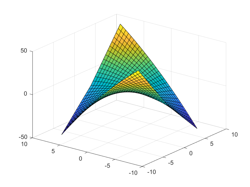
Figure 1: Lagrange function from Example 3.6

To check for inf-sharp condition, we calculate

$$\mathcal{H}_{\mathcal{L}}(x,y)=\mathcal{L}(x,0)-\mathcal{L}(0,y)=|x|+\frac{y^{2}}{8},$$

and check for the value of $\mu>0$ such that for all $(x,y)\in X\times Y$,

$$\mathcal{H}_{\mathcal{L}}(x,y)-\mu\sqrt{x^{2}+y^{2}}>0.$$ (24)

We test $\mu=1,0.5,0.1$. To see the area of interest, we plot the contour of (24) in Figure 2.

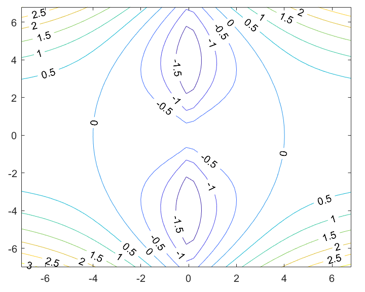
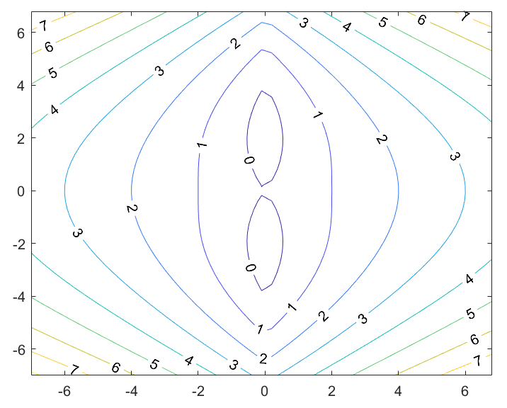
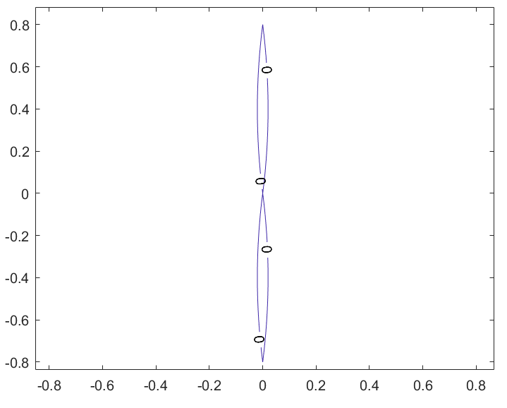
Figure 2: Example 3.6; From left to right: contour plots of $\mathcal{H}_{\mathcal{L}}(x,y)-\mu\sqrt{x^{2}+y^{2}}$ at $\mu=1,0.5,0.1$.

As we can see, Lagrangian is not inf-sharp around $(0,0)$ with $\mu=1$. As we decrease $\mu$, we gain more area for which $\mathcal{H}_{\mathcal{L}}(x,y)-\mu\sqrt{x^{2}+y^{2}}>0$ around $(0,0)$ but never a full neighborhood of $(0,0)$ (even with $\mu=0.1$). Hence, the Lagrangian in this example is not inf-sharp.

Example 3.7.

Let us consider Example 3.5 with the bilinear term as

$$\mathcal{L}(x,y)=|x|+xy-|y|,$$

which has a saddle point at $(0,0)$. The respective primal and dual problems for this Lagrangian are

$$\inf_{-1\leq x\leq 1}|x|,\quad\sup_{-1\leq y\leq 1}-|y|.$$

We calculate the function $\mathcal{H}(x,y)$

$$\mathcal{H}_{\mathcal{L}}(x,y)=\mathcal{L}(x,0)-\mathcal{L}(0,y)=|x|+|y|\geq\sqrt{x^{2}+y^{2}}=\text{dist}((x,y),(0,0)).$$

Therefore, the Lagrangian in this case is inf-sharp with constant $1$. We also illustrate the difference $\mathcal{H}_{\mathcal{L}}(x,y)-\mu\text{dist}((x,y),S$ for $\mu=0.5,0.9,1$ in Figure 3.

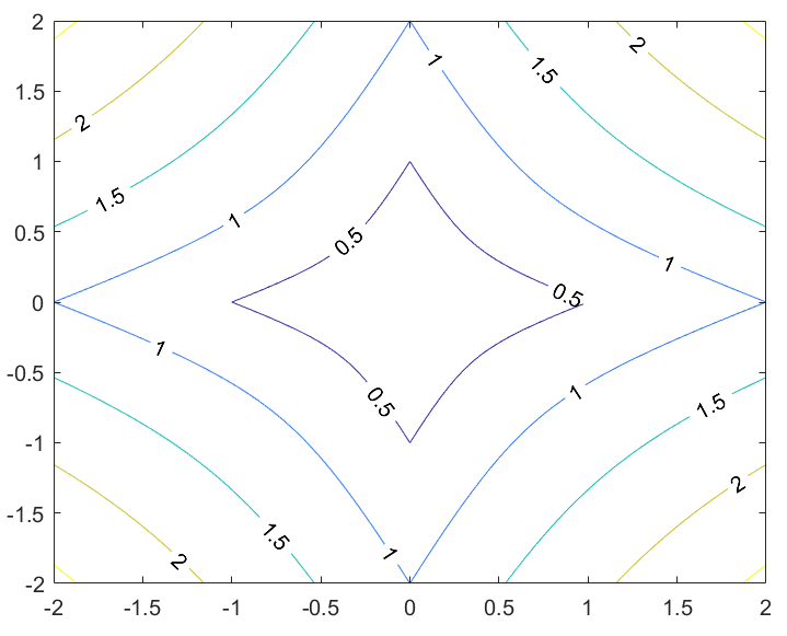
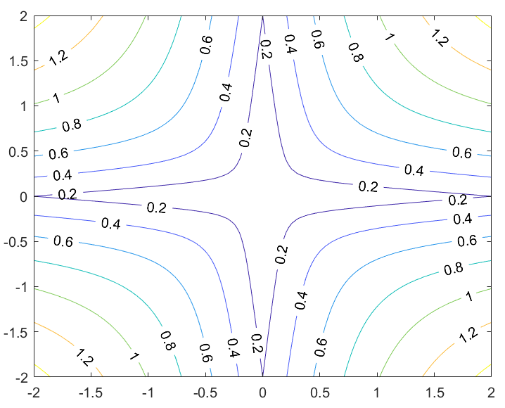
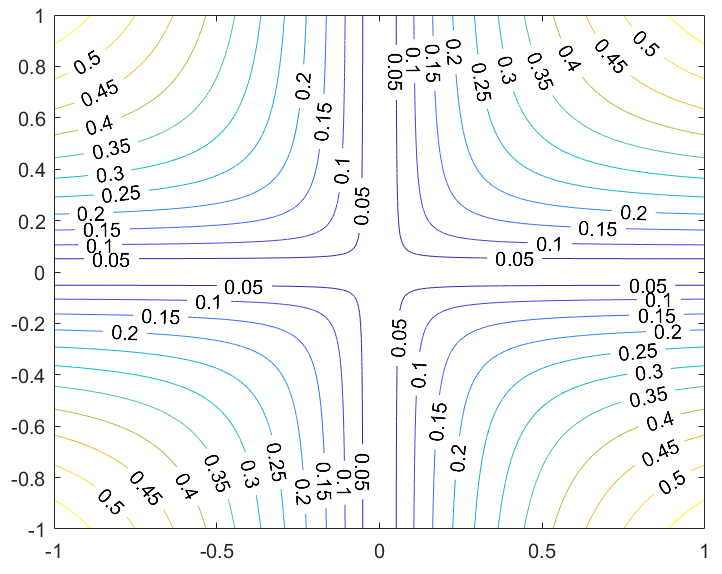
Figure 3: Example 3.7; From left to right: contour plots of $\mathcal{H}_{\mathcal{L}}(x,y)-\mu\text{dist}((x,y),(0,0))$ at $\mu=0.5,0.9,1$.

Example 3.8.

We give one more example of a more complex function. Consider the function

$$\mathcal{K}(x,y)=|x|+|x^{2}-1|+xy-|y|-|y^{2}-1|,$$

which has a saddle point at $(0,0)$ (see Figure 4). The function $\mathcal{K}(x,y)$ is weakly convex in $x$ and weakly concave in $y$.

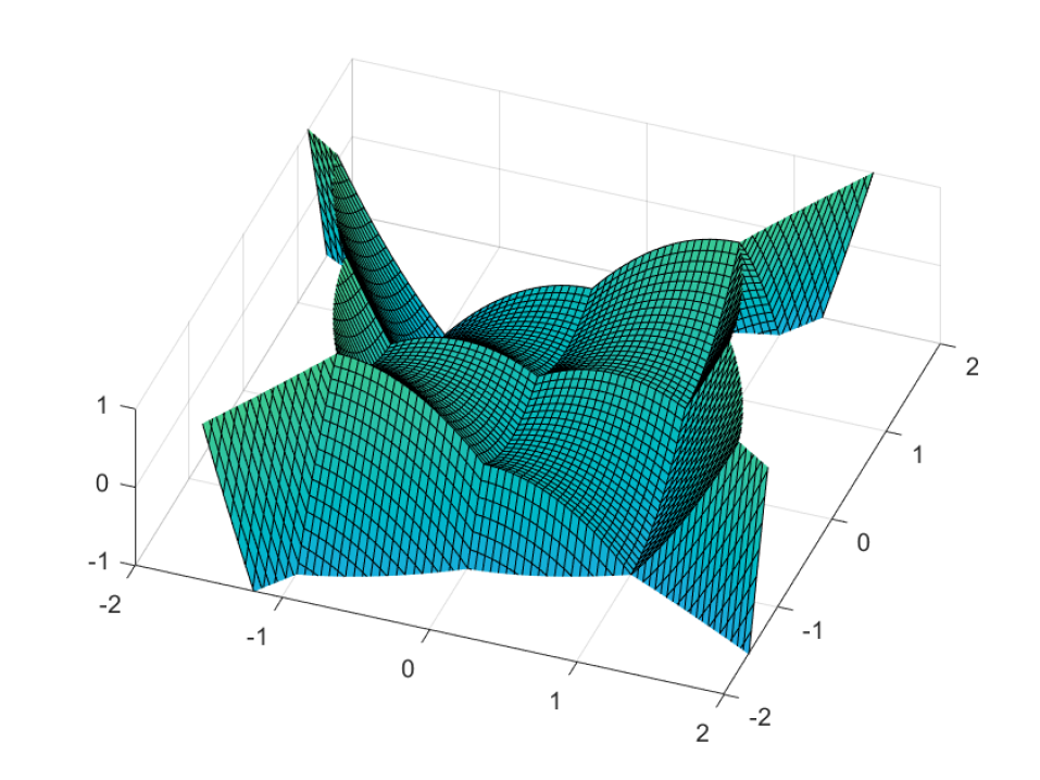
Figure 4: Function $\mathcal{K}(x,y)$ from Example 3.8.

We calculate the function $\mathcal{H}_{\mathcal{K}}(x,y)$

$$\mathcal{H}_{\mathcal{K}}(x,y)=\mathcal{K}(x,0)-\mathcal{K}(0,y) =|x|+|x^{2}-1|+|y|+|y^{2}-1|-2\geq\sqrt{x^{2}+y^{2}}-2=\text{dist}((x,y),(0,0))-2.$$

The above inequality implies that $\mathcal{K}$ is not inf-sharp with constant $1$. In fact, it is locally inf-sharp with constant $\mu<1$. We illustrate the difference $\mathcal{H}_{\mathcal{K}}(x,y)-\mu\text{dist}((x,y),(0,0))$ with $\mu=0.5,0.9,1$ in Figure 5. Notice that there are others points other than the saddle point that $\mathcal{H}_{\mathcal{K}}(x,y)=0$, e.g., $\mathcal{H}_{\mathcal{K}}(0,1)=\mathcal{H}_{\mathcal{K}}(1,1)=\mathcal{H}_{\mathcal{K}}(1,0)=0$.

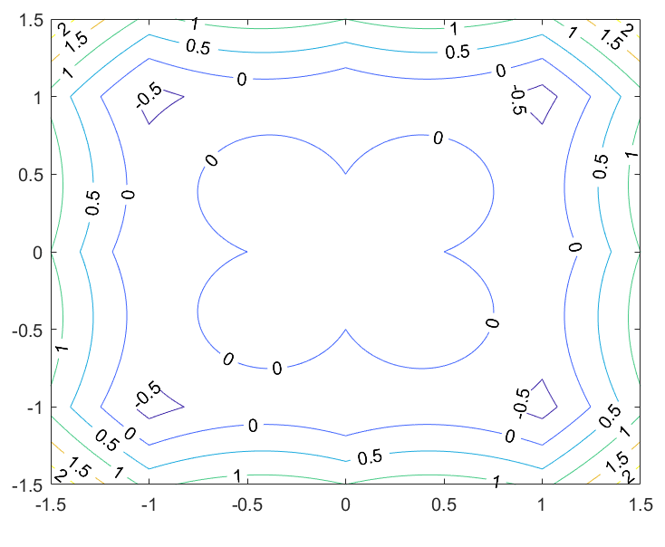
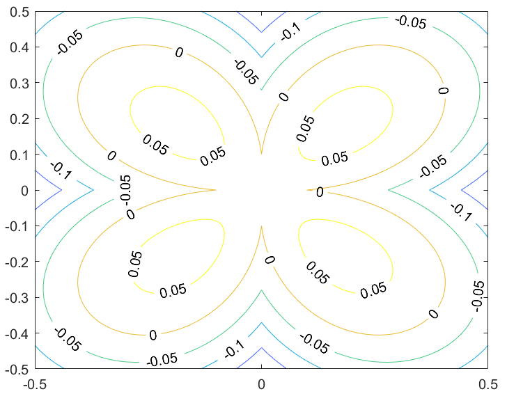
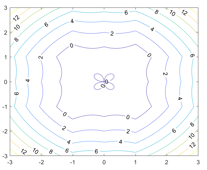
Figure 5: Example 3.8; From left to right: contour plots of $\mathcal{H}_{\mathcal{K}}(x,y)-\mu\text{dist}((x,y),(0,0))$ at $\mu=0.5,0.9,1$.

4 Primal-Dual algorithm with Dual Update

Let us recall the Lagrange saddle point problem (8)

$$\inf_{x\in X}\sup_{y\in Y}f(x)+\langle Lx,y\rangle-g^{*}(y)=\inf_{x\in X}f(x)+g(Lx),$$

where $f$ is proper lsc $\rho$-weakly convex function and $g$ is proper lsc convex defined on Hilbert spaces $X$ and $Y$, respectively, and $L:X\to Y$ is a bounded linear operator with the adjoint operator $L^{*}:Y\to X$. Our standing assumption in this section is that $\text{dom}\,f\cap\text{dom}\,g\circ L\neq\emptyset$ and the set of saddle points $S$ is nonempty.

For convex functions $f$ and $g$, the analogous of Algorithm 1 has been studied in Chambolle and Pock (2011). In He et al. (2014), the authors consider Algorithm 1 for convex case with no relaxation ($\theta=0$). They emphasize that the algorithm may diverge even if the Lagrangian is convex-concave.

In our setting, under the inf-sharpness condition defined in Definition 3.4, we investigate the convergence of Algorithm 1 where function $f$ is weakly convex and $g$ is convex (see Theorem 4.16). For weakly convex function $f$, we use proximal subdifferentials. It has been proved that for this particular class of functions, the proximal subdifferential can be globalized (see (Jourani, 1996, Proposition 3.1)).

1:Initialize: $x_{0}\in\text{dom}\,f\cap\text{dom}\,g\circ L$ and $\bar{y}_{0}=y_{0}$

2:Set: $\tau,\sigma>0,\sigma\rho<1,\theta\in[0,1],\sqrt{\sigma\tau}\|L\|<1$

3:for $n\in\geq 0$ do

4:     $y_{n+1}=\text{argmin}_{y\in Y}g^{*}(y)+\frac{1}{2\tau}\|y-y_{n}-\tau Lx_{n}\|^{2}$ $\triangleright$ (dual update)

5:     $\bar{y}_{n+1}=y_{n+1}+\theta(y_{n+1}-y_{n})$ $\triangleright$ ($\theta$ relaxation step)

6:     $x_{n+1}=\text{argmin}_{x\in X}f(x)+\frac{1}{2\sigma}\|x-x_{n}+\sigma L^{*}\bar{y}_{n+1}\|^{2}$ $\triangleright$ (primal update)

7:end for

Algorithm 1 Primal-Dual Algorithm

In each step of Algorithm 1, we have to solve two minimization problems where the objectives are convex thanks to the appropriate choice of stepsize $\sigma\rho<1$,

$$0\in\partial\left(g^{*}+\frac{1}{2\tau}\|\cdot-y_{n}-\tau Lx_{n}\|^{2}\right)(y_{n+1}),$$ (25)

$$0\in\partial\left(f+\frac{1}{2\sigma}\|\cdot-x_{n}+\sigma L^{*}\bar{y}_{n+1}\|^{2}\right)(x_{n+1}),$$ (26)

where $\partial$ is the subdifferential in the sense of convex analysis. We can apply the convex subdifferentials sum rule to the dual update (25) as both functions are convex (Bauschke and Combettes, 2017, Corollary 16.48). Equivalently, since $\sigma\rho<1$ and $f$ is weakly convex, we utilize the sum rule for proximal subdifferentials for weakly convex function in Theorem 1 with $\varepsilon=0$ to (26), we obtain

$$\frac{y_{n}-y_{n+1}}{\tau}+Lx_{n} \in\partial g^{*}\left(y_{n+1}\right),$$ (27)

$$\frac{x_{n}-x_{n+1}}{\sigma}-L^{*}\bar{y}_{n+1} \in\partial_{\rho}f\left(x_{n+1}\right).$$ (28)

Without the condition $\sigma\rho<1$, the above equivalence between (26) and (28) do not hold. For a detailed discussion of the splitting rule of weakly convex functions, the reader is referred to the work of Bednarczuk et al. (2023a).

Let us estimate the Lagrangian values for the iterates generated by Algorithm 1 for the Lagrangian given in (10).

Proposition 4.9.

Let $X,Y$ be Hilbert spaces, $f:X\to(-\infty,+\infty]$ be proper lsc $\rho$-weakly convex function and $g:Y\to(-\infty,+\infty]$ be proper lsc convex defined on Hilbert spaces $X$ and $Y$, respectively, and $L:X\to Y$ be a bounded linear operator. Let $(x_{n})_{n\in\mathbb{N}},(y_{n})_{n\in\mathbb{N}}$ be the primal and dual sequences generated according to formulas in Algorithm 1. Then for any $(x,y)\in X\times Y$, we have

$$\mathcal{L}\left(x,y_{n+1}\right)-\mathcal{L}\left(x_{n+1},y\right)$$

$$\geq \frac{1-\sqrt{\sigma\tau}\|L\|}{2\tau}\left\|y-y_{n+1}\right\|^{2}-\frac{1}{2\tau}\left\|y-y_{n}\right\|^{2}+\frac{1-\theta\sqrt{\sigma\tau}\|L\|}{2\tau}\left\|y_{n}-y_{n+1}\right\|^{2}$$

$$+\frac{1-\sigma\rho-\theta\sqrt{\sigma\tau}\|L\|}{2\sigma}\left\|x-x_{n+1}\right\|^{2}-\frac{1}{2\sigma}\left\|x-x_{n}\right\|^{2}+\frac{1-\sqrt{\sigma\tau}\|L\|}{2\sigma}\left\|x_{n}-x_{n+1}\right\|^{2}.$$ (29)

Proof 4.10.

From the update of Algorithm 1 and (28), by definitions of subdifferentials, we have

$$(\forall x\in X)\ f(x)-f(x_{n+1}) \geq\frac{1}{\sigma}\langle x_{n}-x_{n+1},x-x_{n+1}\rangle-\langle L^{*}\bar{y}_{n+1},x-x_{n+1}\rangle-\frac{\rho}{2}\|x-x_{n+1}\|^{2},$$

$$(\forall y\in Y)\ g^{*}(y)-g^{*}(y_{n+1}) \geq\frac{1}{\tau}\langle y_{n}-y_{n+1},y-y_{n+1}\rangle+\langle Lx_{n},y-y_{n+1}\rangle,$$

Summing the above inequalities and taking into account the Lagrangian given in (10), we have

$$\mathcal{L}\left(x,y_{n+1}\right)-\mathcal{L}\left(x_{n+1},y\right)$$

$$\geq \left\langle\frac{y_{n}-y_{n+1}}{\tau},y-y_{n+1}\right\rangle+\left\langle\frac{x_{n}-x_{n+1}}{\sigma},x-x_{n+1}\right\rangle-\frac{\rho}{2}\left\|x-x_{n+1}\right\|^{2}$$

$$+\langle L(x_{n}-x_{n+1}),y-y_{n+1}\rangle+\langle L(x-x_{n+1}),y_{n+1}-\bar{y}_{n+1}\rangle,$$

$$= \left\langle\frac{y_{n}-y_{n+1}}{\tau},y-y_{n+1}\right\rangle+\left\langle\frac{x_{n}-x_{n+1}}{\sigma},x-x_{n+1}\right\rangle-\frac{\rho}{2}\left\|x-x_{n+1}\right\|^{2}$$

$$+\langle L\left(x_{n}-x_{n+1}\right),y-y_{n+1}\rangle+\theta\langle L\left({x}-x_{n+1}\right),y_{n}-y_{n+1}\rangle$$ (30)

$$\geq \left\langle\frac{y_{n}-y_{n+1}}{\tau},y-y_{n+1}\right\rangle+\left\langle\frac{x_{n}-x_{n+1}}{\sigma},x-x_{n+1}\right\rangle-\frac{\rho}{2}\left\|x-x_{n+1}\right\|^{2}$$

$$-\sqrt{\sigma\tau}\|L\|\left(\frac{\|x_{n}-x_{n+1}\|^{2}}{2\sigma}+\frac{\|y-y_{n+1}\|^{2}}{2\tau}+\theta\frac{\|x-x_{n+1}\|^{2}}{2\sigma}+\theta\frac{\|y_{n}-y_{n+1}\|^{2}}{2\tau}\right)$$

$$= \frac{1-\sqrt{\sigma\tau}\|L\|}{2\tau}\left\|y-y_{n+1}\right\|^{2}-\frac{1}{2\tau}\left\|y-y_{n}\right\|^{2}+\frac{1-\theta\sqrt{\sigma\tau}\|L\|}{2\tau}\left\|y_{n}-y_{n+1}\right\|^{2}$$

$$+\frac{1-\sigma\rho-\theta\sqrt{\sigma\tau}\|L\|}{2\sigma}\left\|x-x_{n+1}\right\|^{2}-\frac{1}{2\sigma}\left\|x-x_{n}\right\|^{2}+\frac{1-\sqrt{\sigma\tau}\|L\|}{2\sigma}\left\|x_{n}-x_{n+1}\right\|^{2},$$

which is (29).

Noted that we only require $\sigma\rho<1$ in Proposition 4.9 to solve a convex minimization sub-problem in the primal update of Algorithm 1. To investigate the convergence of Algorithm 1, we will utilize the inf-sharpness assumption and estimation (29). We show that if $(x_{n},y_{n})$ are close enough to the solution set $S$, then we have decreasing property for the distance of $(x_{n},y_{n})$ to the set $S$.

Proposition 4.11.

Let $X$ and $Y$ be Hilbert, $f:X\to(-\infty,+\infty]$ be a proper lsc $\rho$-weakly convex function, $g:Y\to(-\infty,+\infty]$ be proper lsc convex and $L:X\to Y$ be a bounded linear operator. Let $(x_{n})_{n\in\mathbb{N}},(y_{n})_{n\in\mathbb{N}}$ be the sequences generated by Algorithm 1. Let us assume that the stepsizes $\tau,\sigma$ satisfy the inequality $\sigma\rho+\theta\sqrt{\sigma\tau}\|L\|<1$, where $\theta\in[0,1]$, and the Lagrangian is inf-sharp in the sense of Definition 3.4 with respect to the set of saddle point $S\neq\emptyset$. At iteration $n\in\mathbb{N}$, we have

$$\text{dist}((x_{n},y_{n}),S)\leq\frac{\mu}{\max\left\{\frac{1}{2\sigma},\frac{1}{2\tau}\right\}-A}\ \Longrightarrow\ \text{dist}((x_{n+1},y_{n+1}),S)\leq\frac{\mu}{\max\left\{\frac{1}{2\sigma},\frac{1}{2\tau}\right\}-A},$$ (31)

where $A:=\min\left\{\frac{1-\sqrt{\sigma\tau}\|L\|}{2\tau},\frac{1-\sigma\rho-\theta\sqrt{\sigma\tau}\|L\|}{2\sigma}\right\}$. Moreover,

$$\text{dist}((x_{n},y_{n}),S)\geq\text{dist}((x_{n+1},y_{n+1}),S).$$ (32)

Proof 4.12.

Let us prove (32) first. By (29) from Proposition 4.9, for any $(x,y)\in X\times Y$, we have

$$\mathcal{L}\left(x,y_{n+1}\right)-\mathcal{L}\left(x_{n+1},y\right)+\frac{1}{2\sigma}\left\|x-x_{n}\right\|^{2}+\frac{1}{2\tau}\left\|y-y_{n}\right\|^{2}$$

$$\geq \frac{1-\sqrt{\sigma\tau}\|L\|}{2\tau}\left\|y-y_{n+1}\right\|^{2}+\frac{1-\theta\sqrt{\sigma\tau}\|L\|}{2\tau}\left\|y_{n}-y_{n+1}\right\|^{2}$$

$$+\frac{1-\sigma\rho-\theta\sqrt{\sigma\tau}\|L\|}{2\sigma}\left\|x-x_{n+1}\right\|^{2}+\frac{1-\sqrt{\sigma\tau}\|L\|}{2\sigma}\left\|x_{n}-x_{n+1}\right\|^{2}$$

$$\geq \frac{1-\sqrt{\sigma\tau}\|L\|}{2\tau}\left\|y-y_{n+1}\right\|^{2}+\frac{1-\sigma\rho-\theta\sqrt{\sigma\tau}\|L\|}{2\sigma}\left\|x-x_{n+1}\right\|^{2}$$

$$\geq A\inf_{(x,y)\in S}\left\|x-x_{n+1}\right\|^{2}+\left\|y-y_{n+1}\right\|^{2}=A\text{dist}^{2}((x_{n+1},y_{n+1}),S),$$ (33)

where $A:=\min\left\{\frac{1-\sqrt{\sigma\tau}\|L\|}{2\tau},\frac{1-\sigma\rho-\theta\sqrt{\sigma\tau}\|L\|}{2\sigma}\right\}>0$ thanks to the assumption on the stepsizes. The last inequality in (33) holds as we can take any $(x,y)\in S$. Rearrange both sides of (33), we obtain

$$\frac{1}{2\sigma}\left\|x-x_{n}\right\|^{2}+\frac{1}{2\tau}\left\|y-y_{n}\right\|^{2}\geq A\text{dist}^{2}((x_{n+1},y_{n+1}),S)+\mathcal{L}\left(x_{n+1},y\right)-\mathcal{L}\left(x,y_{n+1}\right).$$ (34)

Let us take infimum on both sides of (34) with respect to $(x,y)\in S$, we obtain

$$\max\left\{\frac{1}{2\sigma},\frac{1}{2\tau}\right\}\text{dist}^{2}((x_{n},y_{n}),S) \geq A\text{dist}^{2}((x_{n+1},y_{n+1}),S)+\underbrace{\inf_{(x,y)\in S}\left\{\mathcal{L}\left(x_{n+1},y\right)-\mathcal{L}\left(x,y_{n+1}\right)\right\}}_{=\mathcal{H}_{\mathcal{L}}(x_{n+1},y_{n+1})}.$$ (35)

We apply sharpness assumption to (35) and obtain

$$\max\left\{\frac{1}{2\sigma},\frac{1}{2\tau}\right\}\text{dist}^{2}((x_{n},y_{n}),S)\geq A\text{dist}^{2}((x_{n+1},y_{n+1}),S)+\mu\text{dist}((x_{n+1},y_{n+1}),S).$$ (36)

To obtain (32), we need

$$A\text{dist}^{2}((x_{n+1},y_{n+1}),S)+\mu\text{dist}((x_{n+1},y_{n+1}),S) \geq\max\left\{\frac{1}{2\sigma},\frac{1}{2\tau}\right\}\text{dist}^{2}((x_{n+1},y_{n+1}),S),$$

which holds when

$$\text{dist}((x_{n+1},y_{n+1}),S)\leq\frac{\mu}{\max\left\{\frac{1}{2\sigma},\frac{1}{2\tau}\right\}-A}.$$ (37)

The quantity on RHS of (37) is well-defined as

$$\max\left\{\frac{1}{2\sigma},\frac{1}{2\tau}\right\}\geq\min\left\{\frac{1}{2\sigma},\frac{1}{2\tau}\right\}>\min\left\{\frac{1-\sqrt{\sigma\tau}\|L\|}{2\tau},\frac{1-\sigma\rho-\theta\sqrt{\sigma\tau}\|L\|}{2\sigma}\right\},$$

thanks to the assumptions on the stepsizes $\tau,\sigma$. Next, we will prove that for any $n\in\mathbb{N}$

$$\text{dist}((x_{n},y_{n}),S)\leq\frac{\mu}{\max\left\{\frac{1}{2\sigma},\frac{1}{2\tau}\right\}-A}\Rightarrow\text{dist}((x_{n+1},y_{n+1}),S)\leq\frac{\mu}{\max\left\{\frac{1}{2\sigma},\frac{1}{2\tau}\right\}-A}.$$

Let us start from (36)

$$\max\left\{\frac{1}{2\sigma},\frac{1}{2\tau}\right\}\frac{\mu^{2}}{\left(\max\left\{\frac{1}{2\sigma},\frac{1}{2\tau}\right\}-A\right)^{2}} \geq\max\left\{\frac{1}{2\sigma},\frac{1}{2\tau}\right\}\text{dist}^{2}((x_{n},y_{n}),S)$$

$$\geq A\text{dist}^{2}((x_{n+1},y_{n+1}),S)+\mu\text{dist}((x_{n+1},y_{n+1}),S).$$ (38)

Inequality (38) becomes a quadratic inequality with respect to $\text{dist}((x_{n+1},y_{n+1}),S)$. The quadratic equation taken from (38) has two distinct solutions, which implies that

$$0\leq\text{dist}((x_{n+1},y_{n+1}),S)\leq\frac{\mu}{\max\left\{\frac{1}{2\sigma},\frac{1}{2\tau}\right\}-A}.$$

Remark 4.13.

When the iterates are close enough to the solution $S$, the sharpness of order $1$ implies the sharpness of order $2$, which is known as the quadratic growth condition. It has been shown in (Liao et al., 2024, Theorem 3.1) that for a weakly convex function (see formula (18) for the weak convexity of the duality gap function $\mathcal{G}_{\mathcal{L}}$), quadratic growth condition is equivalent to subdifferential error bound and PŁ inequality, which are well-known regularity conditions used to achieve linear convergence rate. On the other hand, inf-sharpness of function $\mathcal{H}_{\mathcal{L}}$ (Definition 3.4) implies sharpness of order $1$ of function $\mathcal{H}_{\mathcal{L}}$.

When inequality in (31) is strict, we obtain convergence of the distance function.

Corollary 4.14.

Let $X$ and $Y$ be Hilbert, $f:X\to(-\infty,+\infty]$ be a proper lsc $\rho$-weakly convex function, $g:Y\to(-\infty,+\infty]$ be proper lsc convex and $L:X\to Y$ be a bounded linear operator. Let $(x_{n})_{n\in\mathbb{N}},(y_{n})_{n\in\mathbb{N}}$ be the sequences generated by Algorithm 1. Let us assume that $\sigma\rho+\theta\sqrt{\sigma\tau}\|L\|<1$ and the Lagrangian is inf-sharp in the sense of Definition 3.4 with respect to the set of saddle points $S\neq\emptyset$. If the starting point $(x_{0},y_{0})$ satisfies

$$\text{dist}((x_{0},y_{0}),S)<\frac{\mu}{\max\left\{\frac{1}{2\sigma},\frac{1}{2\tau}\right\}-A},$$

where $A=\min\left\{\frac{1-\sqrt{\sigma\tau}\|L\|}{2\tau},\frac{1-\sigma\rho-\theta\sqrt{\sigma\tau}\|L\|}{2\sigma}\right\}$. Then $\text{dist}((x_{n},y_{n}),S)$ tends to zero as $n\to\infty$.

Proof 4.15.

By assumption and Proposition 4.11, $\text{dist}((x_{n},y_{n}),S)$ is non-increasing and

$$\text{dist}((x_{n},y_{n}),S)<\frac{\mu}{\max\left\{\frac{1}{2\sigma},\frac{1}{2\tau}\right\}-A},$$

for all $n\in\mathbb{N}$. Moreover, we have

$$\left(A+\frac{\mu}{\text{dist}((x_{0},y_{0}),S)}\right)\text{dist}^{2}((x_{n+1},y_{n+1}),S) \leq\left(A+\frac{\mu}{\text{dist}((x_{n+1},y_{n+1}),S)}\right)\text{dist}^{2}((x_{n+1},y_{n+1}),S)$$

$$\leq\max\left\{\frac{1}{2\sigma},\frac{1}{2\tau}\right\}\text{dist}^{2}((x_{n},y_{n}),S).$$ (39)

Inequality (39) implies that

$$\text{dist}^{2}((x_{n+1},y_{n+1}),S)\leq(B)^{n-1}\text{dist}^{2}((x_{0},y_{0}),S),$$ (40)

where $B:=\frac{\max\left\{\frac{1}{2\sigma},\frac{1}{2\tau}\right\}}{A+\frac{\mu}{\text{dist}((x_{0},y_{0}),S)}}.$ By assumption on $\text{dist}((x_{0},y_{0}),S)$, we have $0<B<1$ since

$$A+\frac{\mu}{\text{dist}((x_{0},y_{0}),S)}>\max\left\{\frac{1}{2\sigma},\frac{1}{2\tau}\right\}.$$

As (40) holds for any $n\in\mathbb{N}$, we let $n\to\infty$ and we infer that

$$\lim_{n\to\infty}\text{dist}((x_{n},y_{n}),S)=0.$$

Next, we prove the convergence of $(x_{n},y_{n})_{n\in\mathbb{N}}$ to a saddle point in $S$.

Theorem 4.16.

Let $X$ and $Y$ be Hilbert, $f:X\to(-\infty,+\infty]$ be a proper lsc $\rho$-weakly convex function, $g:Y\to(-\infty,+\infty]$ be proper lsc convex and $L:X\to Y$ be a bounded linear operator. Let $(x_{n})_{n\in\mathbb{N}},(y_{n})_{n\in\mathbb{N}}$ be the sequences generated by Algorithm 1. Let us assume that the stepsizes $\tau,\sigma$ satisfy $\sigma\rho+\theta\sqrt{\sigma\tau}\|L\|<1$, and the Lagrangian is inf-sharp in the sense of Definition 3.4 with respect to the set of saddle point $S\neq\emptyset$. If the starting point $(x_{0},y_{0})$ satisfies

$$\text{dist}((x_{0},y_{0}),S)<\frac{\mu}{\max\left\{\frac{1}{2\sigma},\frac{1}{2\tau}\right\}-A},$$

where $A=\min\left\{\frac{1-\sqrt{\sigma\tau}\|L\|}{2\tau},\frac{1-\sigma\rho-\theta\sqrt{\sigma\tau}\|L\|}{2\sigma}\right\}.$ Then $(x_{n},y_{n})$ converges to a saddle point.

Proof 4.17.

By (29) from Proposition 4.9 and the inf-sharpness of Lagrangian, we have

$$\max\left\{\frac{1}{2\sigma},\frac{1}{2\tau}\right\}\text{dist}^{2}((x_{n},y_{n}),S)$$

$$\geq A\text{dist}^{2}((x_{n+1},y_{n+1}),S)+\mu\text{dist}((x_{n+1},y_{n+1}),S)$$

$$+\frac{1-\theta\sqrt{\sigma\tau}\|L\|}{2\tau}\left\|y_{n}-y_{n+1}\right\|^{2}+\frac{1-\sqrt{\sigma\tau}\|L\|}{2\sigma}\left\|x_{n}-x_{n+1}\right\|^{2}$$

$$\geq\min\left\{\frac{1-\theta\sqrt{\sigma\tau}\|L\|}{2\tau},\frac{1-\sqrt{\sigma\tau}\|L\|}{2\sigma}\right\}\|(x_{n},y_{n})-(x_{n+1},y_{n+1})\|^{2}_{X\times Y}.$$ (41)

Taking square root on both sides of (41) and summing up till $N\in\mathbb{N}$, combining with the result from Corollary 4.14, we obtain

$$C\sum_{i=0}^{N}B^{\frac{i-1}{2}} \geq\sum_{i=0}^{N}\|(x_{i},y_{i})-(x_{i+1},y_{i+1})\|_{X\times Y},$$ (42)

where

$$B=\frac{\max\left\{\frac{1}{2\sigma},\frac{1}{2\tau}\right\}}{A+\frac{\mu}{\text{dist}((x_{0},y_{0}),S)}},\quad C:=\sqrt{\frac{\max\left\{\frac{1}{2\sigma},\frac{1}{2\tau}\right\}}{\min\left\{\frac{1-\theta\sqrt{\sigma\tau}\|L\|}{2\tau},\frac{1-\sqrt{\sigma\tau}\|L\|}{2\sigma}\right\}}}\text{dist}((x_{0},y_{0}),S).$$

From the proof of Corollary 4.14 we have $0<B<1$. Letting $N\to\infty$, the LHS of (42) is summable which implies that

$$\sum_{i}\|(x_{i},y_{i})-(x_{i+1},y_{i+1})\|_{X\times Y}<+\infty.$$

As $X,Y$ are Hilbert, so is $X\times Y$. By (Bolte et al., 2014, Theorem 1), $(x_{n},y_{n})_{n\in\mathbb{N}}$ is Cauchy , so it converges. Combining this with the result obtained in Corollary 4.14 which is $\text{dist}((x_{n},y_{n}),S)\to 0$ as $n\to\infty$, $(x_{n},y_{n})_{n\in\mathbb{N}}$ must converge to a saddle point in $S$.

5 Primal-Dual algorithm with primal update first

In this section, we consider Algorithm 2, which differs from Algorithm 1 by updating the primal variable $x_{n}$ first instead of $y_{n}$. We show the convergence results similar to Proposition 4.11, and Theorem 4.16 of the previous subsection with some differences concerning the assumption on the stepsizes $\tau,\sigma>0$.

Initialize: $x_{0}\in\text{dom}\,f\cap\text{dom}\,g\circ L$ and $\bar{x}_{0}=x_{0}$

Set: $\tau,\sigma>0,\sigma\rho<1,\theta\in[0,1],\sqrt{\sigma\tau}\|L\|<1$

for For $n\geq 0$ do

     $x_{n+1}=\text{argmin}_{x\in X}f(x)+\frac{1}{2\sigma}\|x-x_{n}+\tau L^{*}{y}_{n}\|^{2}$ $\triangleright$ (primal update)

     $\bar{x}_{n+1}=x_{n+1}+\theta(x_{n+1}-x_{n})$ $\triangleright$ ($\theta$ relaxation step)

     $y_{n+1}=\text{argmin}_{y\in Y}g^{*}(y)+\frac{1}{2\tau}\|y-y_{n}-\tau L\bar{x}_{n+1}\|^{2}$ $\triangleright$ (dual update)

end for

Algorithm 2 Primal-Dual Algorithm with primal update first

Analogously to Proposition 4.9, we start by analyzing the behavior of the Lagrangian values given in (10).

Proposition 5.18.

Let $X,Y$ be Hilbert spaces, $f:X\to(-\infty,+\infty]$ be proper lsc $\rho$-weakly convex function and $g:Y\to(-\infty,+\infty]$ be proper lsc convex defined on Hilbert spaces $X$ and $Y$, respectively, and $L:X\to Y$ be a bounded linear operator. Let $(x_{n})_{n\in\mathbb{N}},(y_{n})_{n\in\mathbb{N}}$ be sequences generated by Algorithm 2. Then for any $(x,y)\in X\times Y$, we have

$$\mathcal{L}\left(x,y_{n+1}\right)-\mathcal{L}\left(x_{n+1},y\right)$$

$$\geq \frac{1-\theta\sqrt{\sigma\tau}\|L\|}{2\tau}\left\|y-y_{n+1}\right\|^{2}-\frac{1}{2\tau}\left\|y-y_{n}\right\|^{2}+\frac{1-\sqrt{\sigma\tau}\|L\|}{2\tau}\left\|y_{n}-y_{n+1}\right\|^{2}$$

$$+\frac{1-\sigma\rho-\sqrt{\sigma\tau}\|L\|}{2\sigma}\left\|x-x_{n+1}\right\|^{2}-\frac{1}{2\sigma}\left\|x-x_{n}\right\|^{2}+\frac{1-\theta\sqrt{\sigma\tau}\|L\|}{2\sigma}\left\|x_{n}-x_{n+1}\right\|^{2}.$$ (43)

Proof 5.19.

We proceed similarly to the proof of Proposition 4.9.

As we can see, the difference between Proposition 4.9 and Proposition 5.18 is the position of $\theta$ which appears in the term $\|y-y_{n+1}\|^{2}$ instead of $\|x-x_{n+1}\|^{2}$. Which will cause a small change in the bound of $\text{dist}((x_{n},y_{n}),S)$ as we see in the following result.

Proposition 5.20.

Let $X$ and $Y$ be Hilbert, $f:X\to(-\infty,+\infty]$ be a proper lsc $\rho$-weakly convex function, $g:Y\to(-\infty,+\infty]$ be proper lsc convex and $L:X\to Y$ be a bounded linear operator. Let $(x_{n})_{n\in\mathbb{N}},(y_{n})_{n\in\mathbb{N}}$ be the sequences generated by Algorithm 2. Let us assume that the stepsizes $\tau,\sigma$ satisfy $\sigma\rho+\sqrt{\sigma\tau}\|L\|<1$ and the Lagrangian is inf-sharp in the sense of Definition 3.4 with respect to the set of saddle points $S\neq\emptyset$. At iteration $n\in\mathbb{N}$, we have

$$\text{dist}((x_{n},y_{n}),S)\leq\frac{\mu}{\max\left\{\frac{1}{2\sigma},\frac{1}{2\tau}\right\}-A_{1}}\ \Longrightarrow\ \text{dist}((x_{n+1},y_{n+1}),S)\leq\frac{\mu}{\max\left\{\frac{1}{2\sigma},\frac{1}{2\tau}\right\}-A_{1}},$$ (44)

where $A_{1}:=\min\left\{\frac{1-\theta\sqrt{\sigma\tau}\|L\|}{2\tau},\frac{1-\sigma\rho-\sqrt{\sigma\tau}\|L\|}{2\sigma}\right\}$. Moreover,

$$\text{dist}^{2}((x_{n},y_{n}),S)\geq\text{dist}^{2}((x_{n+1},y_{n+1}),S).$$ (45)

As a consequence, if the initials $(x_{0},y_{0})$, $\text{dist}((x_{0},y_{0}),S)<\frac{\mu}{\max\left\{\frac{1}{2\sigma},\frac{1}{2\tau}\right\}-A_{1}}.$ Then $\text{dist}((x_{n},y_{n}),S)$ tends to zero as $n\to\infty$.

The proof of Proposition 5.20 follows the same lines as the proof of Proposition 4.11 and Corollary 4.14 so we will not give it here. As $(\text{dist}((x_{n},y_{n}),S))_{n\in\mathbb{N}}$ with $(x_{n})_{n\in\mathbb{N}},(y_{n})_{n\in\mathbb{N}}$ generated by Algorithm 2 behaves in the same way as in the case of Algorithm 1, so is the convergence of $(x_{n},y_{n})_{n\in\mathbb{N}}$.

Theorem 5.21.

Let $X$ and $Y$ be Hilbert, $f:X\to(-\infty,+\infty]$ be a proper lsc $\rho$-weakly convex function, $g:Y\to(-\infty,+\infty]$ be proper lsc convex and $L:X\to Y$ be a bounded linear operator. Let $(x_{n})_{n\in\mathbb{N}},(y_{n})_{n\in\mathbb{N}}$ be the sequences generated by Algorithm 2. Let us assume that the stepsizes $\tau,\sigma$ satisfy $\sigma\rho+\sqrt{\sigma\tau}\|L\|<1$ and the Lagrangian is inf-sharp in the sense of Definition 3.4 with respect to the set of saddle point $S\neq\emptyset$. If the starting point $(x_{0},y_{0})$ satisfies

$$\text{dist}((x_{0},y_{0}),S)<\frac{\mu}{\max\left\{\frac{1}{2\sigma},\frac{1}{2\tau}\right\}-A_{1}},$$ (46)

where $A_{1}=\min\left\{\frac{1-\theta\sqrt{\sigma\tau}\|L\|}{2\tau},\frac{1-\sigma\rho-\sqrt{\sigma\tau}\|L\|}{2\sigma}\right\}$. Then $(x_{n},y_{n})$ converges to a saddle point.

The condition (46) gives us the radius of an open ball around the set $S$ such that Algorithm 2 converges to a saddle point, provided that we start inside the ball. When starting outside the ball, the sequences can converge to other points but not the saddle point. We will observe this behavior in the numerical example below.

6 Solution to the Primal Problem

While the inf-sharpness in the sense of Definition 3.4 helps us analyze the convergence of Algorithm 1 and Algorithm 2, one needs to know the set of saddle points (both the primal and dual solutions) to calculate $\mathcal{H}_{\mathcal{K}}(x,y)$. It is interesting to solve problem (2) with only knowledge of the primal objective; hence, we ask ourselves how much we know about the convergence of Algorithm 1 or 2. Is it possible to assume sharpness condition only on the primal objective functions instead of on the Lagrangian, and how is it related to Definition 3.3 and Definition 3.4?

In this section, we consider the same setting as in Section 3, where $f$ is $\rho$-weakly convex and $g$ is convex. We analyze the gap function $\mathcal{G}_{\mathcal{L}}(x,y)$ given by (17) with the Lagrangian given in (10),

$$\mathcal{G}_{\mathcal{L}}(x,y)=\sup_{\overline{x}\in X,\overline{y}\in Y}\mathcal{L}(x,\overline{y})-\mathcal{L}(\overline{x},y)=f(x)+g^{**}(Lx)+g^{*}(y)+\sup_{\overline{x}\in X}\{-\langle L\overline{x},y\rangle-f(\overline{x})\}.$$

Since $g$ is convex, we have $g=g^{**}$. Let us take

$$\inf_{y\in Y}\mathcal{G}_{\mathcal{L}}(x,y) =\inf_{y\in Y}\left\{(f+g\circ L)(x)+\sup_{\overline{x}\in X}\{-\langle L\overline{x},y\rangle-f(\overline{x})+g^{*}(y)\}\right\}$$

$$=(f+g\circ L)(x)-\sup_{y\in Y}\inf_{\overline{x}\in X}\left\{f(\overline{x})+\langle L\overline{x},y\rangle-g^{*}(y)\right\}$$

$$\geq(f+g\circ L)(x)-\inf_{\overline{x}\in X}\sup_{y\in Y}\mathcal{L}(\overline{x},y)$$

$$=(f+g\circ L)(x)-\inf_{\overline{x}\in X}(f+g\circ L)(\overline{x}),$$ (47)

where we use weak duality in the third inequality, and the last equality is the equivalence between Lagrangian primal (8) and primal problem (2) thanks to the convexity of $g$.

Before discussing the convergence of the algorithm, let us give a proper definition of sharpness for problem (2).

Definition 6.22 (Sharpness of Primal Objective).

We say that the objective function $f+g\circ L$ is sharp with respect to the set of minimizers $S_{P}=\underset{\begin{subarray}{c}{}\end{subarray}}{\mathrm{argmin}}\;\;(f+g\circ L)\neq\emptyset$ if there exists a positive constant $\mu$ such that

$$(\forall x\in X)\quad(f+g\circ L)(x)-\inf_{z\in X}(f+g\circ L)(z)\geq\mu\text{dist}\left(x,S_{P}\right).$$ (48)

Similarly, we can also define sharpness for the Lagrangian dual problem (9) as follow: there exists $\eta>0$ such that

$$(\forall y_{0}\in Y)\quad\sup_{y\in Y}\inf_{x\in X}\mathcal{L}(x,y)-\inf_{x\in X}\mathcal{L}(x,y_{0})\geq\eta\text{dist}(y_{0},S_{D}),$$ (49)

where $S_{D}=\text{argmax}_{y\in Y}\{\inf_{x\in X}\mathcal{L}(x,y)\}$ is the solution to the dual problem.

The relationship between the sharpness of the primal problem and the sharpness of Lagrangian is described in the next proposition.

Proposition 6.23.

Let us consider the composite problem (2) and its corresponding Lagrangian given in (10). If the Lagrangian is sharp in the sense of Definition 3.3 then the primal objective function is sharp as in Definition 6.22. On the other hand, if the objective primal $f+g\circ L$ is sharp according to Definition 6.22 and the respective Lagrange dual is sharp as in (49) then there exists $\xi>0$ such that

$$\mathcal{G}_{\mathcal{L}}(x,y)\geq\xi(\text{dist}(x,S_{P})+\text{dist}(y,S_{D})),$$

where $S_{P},S_{D}$ are the solution sets of the primal (6.22) and dual (49) problems, respectively.

Proof 6.24.

By Definition 3.3, we have

$$\mathcal{G}_{\mathcal{L}}(x,y)=f(x)+g^{*}(y)+\sup_{(\hat{x},\hat{y})\in X\times Y}\langle Lx,\hat{y}\rangle-\langle L\hat{x},y\rangle-f(\hat{x})-g^{*}(\hat{y})\geq\mu\text{dist}((x,y),S),$$

where $S$ is the set of saddle points. The RHS of the above inequality can be written

$$\text{dist}((x,y),S) =\inf_{(\bar{x},\bar{y})\in S}\|(x,y)-(\bar{x},\bar{y})\|_{X\times Y}=\inf_{(\bar{x},\bar{y})\in S}\sqrt{\|x-\bar{x}\|_{X}^{2}+\|y-\bar{y}\|^{2}_{Y}}$$

$$\geq\inf_{(\bar{x},\bar{y})\in S}\|x-\bar{x}\|_{X}\geq\text{dist}(x,S_{P}).$$ (50)

On the other hand, observe that

$$\mathcal{G}_{\mathcal{L}}(x,y) =f(x)+g^{*}(y)+\sup_{(\hat{x},\hat{y})\in X\times Y}\left\{\langle Lx,\hat{y}\rangle-\langle L\hat{x},y\rangle-f(\hat{x})-g^{*}(\hat{y})\right\}$$

$$=f(x)+g^{*}(y)+\sup_{\hat{x}\in X}\left\{-\langle L\hat{x},y\rangle-f(\hat{x})\right\}+\sup_{\hat{y}\in Y}\left\{\langle Lx,\hat{y}\rangle-g^{*}(\hat{y})\right\}$$

$$=f(x)+g^{*}(y)+g^{**}(Lx)+\sup_{\hat{x}\in X}\left\{-\langle L\hat{x},y\rangle-f(\hat{x})\right\}$$

$$=f(x)+g(Lx)+\sup_{\hat{x}\in X}\left\{-\langle L\hat{x},y\rangle-f(\hat{x})+g^{*}(y)\right\}.$$ (51)

Combining (50) and (51)

$$f(x)+g(Lx)+\sup_{\hat{x}\in X}\left\{-\langle L\hat{x},y\rangle-f(\hat{x})+g^{*}(y)\right\}\geq\mu\text{dist}(x,S_{P}).$$ (52)

Since (52) holds for any $(x,y)\in X\times Y$, we fix $y=y^{*}$ as a saddle point and obtain

$$(f+g\circ L)(x)-\inf_{\hat{x}\in X}\sup_{\hat{y}\in Y}\left\{\langle L\hat{x},\hat{y}\rangle+f(\hat{x})-g^{*}(\hat{y})\right\} \geq(f+g\circ L)(x)-\inf_{\hat{x}\in X}\left\{f(\hat{x})+\langle L\hat{x},y^{*}\rangle-g^{*}(y^{*})\right\}$$

$$\geq\mu\text{dist}(x,S_{P}).$$

Thanks to the convexity of $g$, the Lagrange primal has the same value as problem (2). Hence, we obtain

$$(f+g\circ L)(x)-\inf_{\hat{x}\in X}(f+g\circ L)(\hat{x})\geq\mu\text{dist}(x,S_{P}).$$

For the second statement, let us assume that $f+g\circ L$ is sharp, then there exists $\mu\geq 0$ such that

$$(f+g\circ L)(x)-\inf_{\hat{x}\in X}f(\hat{x})+g(L\hat{x})\geq\mu\text{dist}(x,S_{P}),$$

for any $x_{0}\in X$ and $S_{P}=\text{argmin}f+g\circ L$. We use (47) and obtain

$$\mathcal{G}_{\mathcal{L}}(x,y)\geq\inf_{y\in Y}\mathcal{G}_{\mathcal{L}}(x,y)\geq(f+g\circ L)(x)-\inf_{\overline{x}\in X}(f+g\circ L)(\overline{x})\geq\mu\text{dist}(x,S_{P}).$$ (53)

We recall that the dual problem has the form

$$\sup_{y\in Y}\inf_{x\in X}\mathcal{L}(x,y)=\sup_{y\in Y}-f^{*}(-L^{*}y)-g^{*}(y),$$

then sharpness for the objective of the dual problem as in (49) is

$$(\exists\eta>0)(\forall y\in Y)\quad\sup_{\hat{y}\in Y}-f^{*}(-L^{*}\hat{y})-g^{*}(\hat{y})+f^{*}(-L^{*}{y})+g^{*}({y})\geq\eta\text{dist}(y,S_{D}).$$

With the same argument with the primal problem as above, we get the following

$$\mathcal{G}_{\mathcal{L}}(x,y)\geq\eta\text{dist}(y,S_{D}).$$ (54)

Summing (53) and (54),

$$2\mathcal{G}_{\mathcal{L}}(x,y)\geq\mu\text{dist}(x,S_{P})+\eta\text{dist}(y,S_{D}) \geq\min\{\mu,\eta\}\left(\text{dist}(x,S_{P})+\text{dist}(y,S_{D})\right).$$ (55)

Denoting $\xi=\min\{\mu,\eta\}/2$, we finish the proof.

The above proposition shows the relationship between the gap function and the primal problem. For the modified gap function $\mathcal{H}_{\mathcal{L}}(x,y)$, we obtain the following estimation.

Lemma 6.25.

Let us consider the composite problem (2) and its corresponding Lagrangian given in (10). Assume that $f+g\circ L$ is bounded from below, the set of minimizer $S_{P}$ of problem (2), the set of saddle point $S$ of Lagrangian problems are nonempty. For any saddle point $(x^{*},y^{*})\in S$ and $(x,y)\in X\times Y$, the following holds,

$$(f+g\circ L)(x)-\inf(f+g\circ L)\leq\mathcal{L}\left(x,y^{*}\right)-\mathcal{L}\left(x^{*},y\right)+\left\langle Lx-Lx^{*},\overline{y}-y^{*}\right\rangle,$$ (56)

where $\overline{y}\in\partial g(Lx)$. Moreover, if problem (2) is sharp in the sense of Definition 6.22 with $\mu>0$ and $g,g^{*}$ are $\eta$ and $\eta^{-1}$-strongly convex, respectively, with $\eta>0$. Then, we have

$$\mathcal{H}_{\mathcal{L}}(x,y)\geq\mu\text{dist}(x,S_{P}),$$

for all $(x,y)\in X\times Y,y\in\partial g(Lx)$, where $\mathcal{H}(x,y)$ is the modified gap function (21).

Proof 6.26.

Let $x^{*}\in S_{P}$ then for any $y\in Y$, we have

$$-\inf_{\overline{x}\in X}(f+g\circ L)(\overline{x})=-\left(f+g\circ L\right)\left(x^{*}\right) =-\mathcal{L}(x^{*},y)-g(Lx^{*})-g^{*}(y)+\langle Lx^{*},y\rangle.$$

On the other hand, for any $x\in X$, there exists $y^{*}$ corresposding to $x^{*}$ such that $(x^{*},y^{*})\in S$ is a saddle point

$$\left(f+g\circ L\right)\left(x\right) =\mathcal{L}\left(x,y^{*}\right)+g\left(Lx\right)+g^{*}\left(y^{*}\right)-\left\langle Lx,y^{*}\right\rangle.$$

Summing the two and taking $\overline{y}\in\partial g(Lx)$, we obtain

$$\left(f+g\circ L\right)\left(x\right)-\inf\left(f+g\circ L\right)$$

$$=\mathcal{L}(x,y^{*})-\mathcal{L}(x^{*},y)+\left[-g(Lx^{*})-g^{*}(y)+\langle Lx^{*},y\rangle+g\left(Lx\right)+g^{*}\left(y^{*}\right)-\left\langle Lx,y^{*}\right\rangle\right]$$

$$\leq\mathcal{L}(x,y^{*})-\mathcal{L}(x^{*},y)+\left[\langle\overline{y},L(x-x^{*})\rangle+\langle Lx^{*},y^{*}-y\rangle+\langle Lx^{*},y\rangle-\left\langle Lx,y^{*}\right\rangle\right]$$ (57)

$$=\mathcal{L}(x,y^{*})-\mathcal{L}(x^{*},y)+\langle L(x-x^{*}),\overline{y}-y^{*}\rangle.$$

This holds for any $(x,y)\in X\times Y$ and $\overline{y}\in\partial g(Lx)$. Hence, we have (56).

Let us assume that the primal problem (2) is sharp with $\mu>0$ (48), we have

$$\mu\text{dist }\left(x,S_{P}\right)\leq\left(f+g\circ L\right)\left(x\right)-\left(f+g\circ L\right)\left(x^{*}\right)\leq\mathcal{L}\left(x,y^{*}\right)-\mathcal{L}\left(x^{*},y\right)+\left\langle Lx-Lx^{*},\overline{y}-y^{*}\right\rangle,$$

where $\left(x^{*},y^{*}\right)\in S$ is the saddle point. Then taking the infimum w.r.t $\left(x^{*},y^{*}\right)\in S$, we obtain

$$\mu\text{dist }\left(x,S_{P}\right)+\inf_{\left(x^{*},y^{*}\right)\in S}-\left\langle Lx-Lx^{*},\overline{y}-y^{*}\right\rangle\leq\inf_{\left(x^{*},y^{*}\right)\in S}\mathcal{L}\left(x,y^{*}\right)-\mathcal{L}\left(x^{*},y\right)=\mathcal{H}\left(x,y\right)$$

for any $\left(x,y\right)\in X\times Y$.

On the other hand, when both $g^{*}$ and $g$ are $\eta^{-1}$ and $\eta$-strongly convex, respectively, (Bauschke and Combettes, 2017, Proposition 14.2)), from (57), we can have the following form

$$\mu\text{dist }\left(x,S_{P}\right) \leq\mathcal{L}\left(x,y^{*}\right)-\mathcal{L}\left(x^{*},y\right)+\left\langle Lx-Lx^{*},\overline{y}-y^{*}\right\rangle-\frac{1}{2\eta}\|y-y^{*}\|^{2}-\frac{\eta}{2}\|Lx-Lx^{*}\|^{2}$$

$$=\mathcal{L}\left(x,y^{*}\right)-\mathcal{L}\left(x^{*},y\right)-\frac{1}{2\eta}\|y-y^{*}\|^{2}-\frac{\eta}{2}\|Lx-Lx^{*}\|^{2}$$

$$+\frac{1}{2}\left(\alpha\|Lx-Lx^{*}\|^{2}+\frac{1}{\alpha}\|\overline{y}-y^{*}\|^{2}-\|\sqrt{\alpha}{Lx-Lx^{*}}-\frac{\overline{y}-y^{*}}{\sqrt{\alpha}}\|^{2}\right)$$

$$\leq\mathcal{L}\left(x,y^{*}\right)-\mathcal{L}\left(x^{*},y\right)+\frac{1}{2\alpha}\|\overline{y}-y^{*}\|^{2}-\frac{1}{2\eta}\|y-y^{*}\|^{2}+\frac{\alpha-\eta}{2}\|Lx-Lx^{*}\|^{2}$$

$$\leq\mathcal{L}\left(x,y^{*}\right)-\mathcal{L}\left(x^{*},y\right)+\frac{1}{2\alpha}\|\overline{y}-y^{*}\|^{2}-\frac{1}{2\eta}\|y-y^{*}\|^{2}.$$

where $\eta>\alpha>0$. Letting $y=\overline{y}$ and taking the infimum with respect to $(x^{*},y^{*})\in S$, and we finish the proof.

Before using primal sharpness to discuss convergence of primal-dual algorithm, we need to transform the Lagrangian into primal objective. For $(x,y),(x_{0},y_{0})\in X\times Y$, we consider

$$\mathcal{L}(x,y_{0})-\mathcal{L}(x_{0},y) =f(x)-f(x_{0})+g^{*}(y)-g^{*}(y_{0})+\langle Lx,y_{0}\rangle-\langle Lx_{0},y\rangle$$

$$\geq f(x)-f(x_{0})-g^{*}(y_{0})+\langle Lx,y_{0}\rangle-g^{**}(Lx_{0})$$

$$=(f+g\circ L)(x)-(f+g\circ L)(x_{0})-g^{*}(y_{0})+\langle Lx,y_{0}\rangle-g(Lx),$$ (58)

where we utilize the convexity of $g$ in the last equality. Let us fix $(x,y)$ and take $y_{0}\in\partial g(Lx)$, then for any $x_{0}\in X$, (58) becomes

$$\mathcal{L}(x,y_{0})-\mathcal{L}(x_{0},y)\geq(f+g\circ L)(x)-(f+g\circ L)(x_{0}).$$ (59)

Inequality (59) indicates that the choice of $y_{0}$ depends on $x$. For primal-dual algorithms, one often arrive at the term $\mathcal{L}(x_{n+1},y_{0})-\mathcal{L}(x_{0},y_{n+1})$ for any $(x_{0},y_{0})\in X\times Y$, and so we need to know $x_{n+1}$ before choosing $y_{0}$. In this case, Algorithm 2 is more suitable for us as we perform the primal update before the dual. Therefore, we focus on Algorithm 2 in this section. This will be made clearer in the following result.

Proposition 6.27.

Let $X$ and $Y$ be Hilbert, $f:X\to(-\infty,+\infty]$ be a proper lsc $\rho$-weakly convex function, $g:Y\to(-\infty,+\infty]$ be proper lsc convex and $L:X\to Y$ be a bounded linear operator. Let $(x_{n})_{n\in\mathbb{N}},(y_{n})_{n\in\mathbb{N}}$ be the sequences generated by Algorithm 2. Let us assume that the stepsizes $\tau,\sigma$ satisfy the inequality $\sigma\rho+\sqrt{\sigma\tau}\|L\|<1$, and primal objective is sharp as in Definition 6.22 with respect to the set of $S_{P}=\arg\min(f+g\circ L)\neq\emptyset$. Then we have the following,

$$\frac{1}{2\sigma}\text{dist}^{2}(x_{n},S_{P})+\frac{1}{2\tau}\text{dist}^{2}(y_{n},\partial g(Lx_{n+1})) \geq\frac{1-\sigma\rho-\sqrt{\sigma\tau}\|L\|}{2\sigma}\text{dist}^{2}(x_{n+1},S_{P})+\mu\text{dist}(x_{n+1},S_{P}).$$ (60)

Proof 6.28.

Let us recall (43) in Proposition 5.18, for any $(x,y)\in X\times Y$,

$$\mathcal{L}\left(x,y_{n+1}\right)-\mathcal{L}\left(x_{n+1},y\right)$$

$$\geq \frac{1-\theta\sqrt{\sigma\tau}\|L\|}{2\tau}\left\|y-y_{n+1}\right\|^{2}-\frac{1}{2\tau}\left\|y-y_{n}\right\|^{2}+\frac{1-\sqrt{\sigma\tau}\|L\|}{2\tau}\left\|y_{n}-y_{n+1}\right\|^{2}$$

$$+\frac{1-\sigma\rho-\sqrt{\sigma\tau}\|L\|}{2\sigma}\left\|x-x_{n+1}\right\|^{2}-\frac{1}{2\sigma}\left\|x-x_{n}\right\|^{2}+\frac{1-\theta\sqrt{\sigma\tau}\|L\|}{2\sigma}\left\|x_{n}-x_{n+1}\right\|^{2}.$$ (61)

We utilise (59) to obtain

$$\mathcal{L}(x_{n+1},y_{0})-\mathcal{L}(x,y_{n+1})\geq(f+g\circ L)(x_{n+1})-(f+g\circ L)(x),$$ (62)

for any $x\in X$ and $y=y^{*}_{n+1}\in\partial g(Lx_{n+1})$. Combining (62), sharpness condition (48) and take $x^{*}\in S_{P}$, (61) becomes

$$-\mu\text{dist}\left(x_{n+1},S_{P}\right) \geq\frac{1-\theta\sqrt{\sigma\tau}\|L\|}{2\tau}\left\|y^{*}_{n+1}-y_{n+1}\right\|^{2}-\frac{1}{2\tau}\left\|y^{*}_{n+1}-y_{n}\right\|^{2}+\frac{1-\sqrt{\sigma\tau}\|L\|}{2\tau}\left\|y_{n}-y_{n+1}\right\|^{2}$$

$$+\frac{1-\sigma\rho-\sqrt{\sigma\tau}\|L\|}{2\sigma}\left\|x^{*}-x_{n+1}\right\|^{2}-\frac{1}{2\sigma}\left\|x^{*}-x_{n}\right\|^{2}+\frac{1-\theta\sqrt{\sigma\tau}\|L\|}{2\sigma}\left\|x_{n}-x_{n+1}\right\|^{2}.$$

As $y^{*}_{n+1}\in\partial g(Lx_{n+1})$ and $x^{*}\in S_{P}$ can be taken arbitrarily, we obtain

$$-\mu\text{dist}\left(x_{n+1},S_{P}\right) \geq\frac{1-\theta\sqrt{\sigma\tau}\|L\|}{2\tau}\text{dist}^{2}(y_{n+1},\partial g(Lx_{n+1}))-\frac{1}{2\tau}\text{dist}^{2}(y_{n},\partial g(Lx_{n+1}))$$

$$+\frac{1-\sigma\rho-\sqrt{\sigma\tau}\|L\|}{2\sigma}\text{dist}^{2}(x_{n+1},S_{P})-\frac{1}{2\sigma}\text{dist}^{2}(x_{n},S_{P})$$

$$+\frac{1-\sqrt{\sigma\tau}\|L\|}{2\tau}\left\|y_{n}-y_{n+1}\right\|^{2}+\frac{1-\theta\sqrt{\sigma\tau}\|L\|}{2\sigma}\left\|x_{n}-x_{n+1}\right\|^{2}.$$

By assumption on the stepsizes $\tau,\sigma$, we obtain (60).

This shows that the convergence of $(\text{dist}\left(x_{n},S_{P}\right))_{n\in\mathbb{N}}$ depends on the distance of the dual sequence $(y_{n})_{n\in\mathbb{N}}$ to $\partial g(Lx_{n+1})$. This occurs since we only make assumption on the primal objective, and do not have additional information on the dual variable $y\in Y$ like in Definition 3.4. Hence, one can think of the term $(\text{dist}\left(y_{n},\partial g(Lx_{n+1}\right))_{n\in\mathbb{N}}$ as the inexactness produce by the algorithm, despite the fact that proximal calculation is exact. For simplicity, we denote $\varepsilon_{n}:=\text{dist}(y_{n},\partial g(Lx_{n+1}))\geq 0$ for all $n\in\mathbb{N}$. This quantity can be checked after the primal update and with $\varepsilon_{n}$ small enough, we can obtain convergence, as we will see below.

Lemma 6.29.

Let $X$ and $Y$ be Hilbert, $f:X\to(-\infty,+\infty]$ be a proper lsc $\rho$-weakly convex function, $g:Y\to(-\infty,+\infty]$ be proper lsc convex and $L:X\to Y$ be a bounded linear operator. Let $(x_{n})_{n\in\mathbb{N}},(y_{n})_{n\in\mathbb{N}}$ be the sequences generated by Algorithm 2. Let us assume that the stepsizes $\tau,\sigma$ satisfy the inequality $\sigma\rho+\sqrt{\sigma\tau}\|L\|<1$, where $\theta\in[0,1]$, and primal objective is sharp as in Definition 6.22 with respect to the set of $S_{P}=\arg\min(f+g\circ L)\neq\emptyset$. If $\sigma,\tau$ satisfy the following

$$(\forall n\in\mathbb{N})\quad\mu^{2}\sigma\tau>(\sigma\rho+\sqrt{\sigma\tau}\|L\|)\varepsilon_{n}^{2},\ \varepsilon_{n}=\text{dist}(y_{n},\partial g(Lx_{n+1})),$$

and at iteration $n\in\mathbb{N}$,

$$\text{dist}\left(x_{n},S_{P}\right)\leq E^{+}_{n}\quad \Longrightarrow\quad\text{dist}(x_{n+1},S_{P})\leq E^{+}_{n},$$ (63)

$$\text{dist}\left(x_{n},S_{P}\right)\leq E^{-}_{n}\quad \Longrightarrow\quad\text{dist}(x_{n+1},S_{P})\leq E^{-}_{n},$$ (64)

where

$$E_{n}^{+}:=\frac{\sigma\mu+\sigma\sqrt{\mu^{2}-\frac{\varepsilon_{n}^{2}(\sigma\rho+\sqrt{\sigma\tau}\|L\|)}{\sigma\tau}}}{\sigma\rho+\sqrt{\sigma\tau}\|L\|},\quad E_{n}^{-}:=\frac{\sigma\mu-\sigma\sqrt{\mu^{2}-\frac{\varepsilon_{n}^{2}(\sigma\rho+\sqrt{\sigma\tau}\|L\|)}{\sigma\tau}}}{\sigma\rho+\sqrt{\sigma\tau}\|L\|}.$$

Moreover, if

$$E_{n}^{-}\leq\text{dist}(x_{n+1},S_{P})\leq E_{n}^{+},$$ (65)

Then $\text{dist}(x_{n+1},S_{P})\leq\text{dist}(x_{n},S_{P})$.

Proof 6.30.

From (60), we have

$$\frac{1}{2\sigma}\text{dist}^{2}(x_{n},S_{P})\geq\frac{1-\sigma\rho-\sqrt{\sigma\tau}\|L\|}{2\sigma}\text{dist}^{2}(x_{n+1},S_{P})+\mu\text{dist}(x_{n+1},S_{P})-\frac{\varepsilon_{n}^{2}}{2\tau}.$$ (66)

We would like the RHS of (66) satisfies

$$\frac{1-\sigma\rho-\sqrt{\sigma\tau}\|L\|}{2\sigma}\text{dist}^{2}(x_{n+1},S_{P})+\mu\text{dist}(x_{n+1},S_{P})-\frac{\varepsilon_{n}^{2}}{2\tau}\geq\frac{1}{2\sigma}\text{dist}^{2}(x_{n+1},S_{P}),$$

which is equivalent to solving the following quadratic inequality

$$\frac{\sigma\rho+\sqrt{\sigma\tau}\|L\|}{2\sigma}z^{2}-\mu z+\frac{\varepsilon_{n}^{2}}{2\tau}\leq 0.$$

Thanks to the assumption $\mu^{2}\sigma\tau>(\sigma\rho+\sqrt{\sigma\tau}\|L\|)\varepsilon_{n}^{2}$, we obtain the solution

$$\frac{\sigma\mu-\sigma\sqrt{\mu^{2}-\frac{\varepsilon_{n}^{2}(\sigma\rho+\sqrt{\sigma\tau}\|L\|)}{\sigma\tau}}}{\sigma\rho+\sqrt{\sigma\tau}\|L\|}\leq\text{dist}(x_{n+1},S_{P})\leq\frac{\sigma\mu+\sigma\sqrt{\mu^{2}-\frac{\varepsilon_{n}^{2}(\sigma\rho+\sqrt{\sigma\tau}\|L\|)}{\sigma\tau}}}{\sigma\rho+\sqrt{\sigma\tau}\|L\|},$$

which is (65). If (65) holds, we obtain $\text{dist}(x_{n+1},S_{P})\leq\text{dist}(x_{n},S_{P})$.

Let us prove (63), assume that for $n\in\mathbb{N}$, we have $\text{dist}(x_{n},S_{P})\leq E_{n}^{+}$. By (66), we have

$$\frac{1}{2\sigma}(E_{n}^{+})^{2}\geq\frac{1-\sigma\rho-\sqrt{\sigma\tau}\|L\|}{2\sigma}\text{dist}^{2}(x_{n+1},S_{P})+\mu\text{dist}(x_{n+1},S_{P})-\frac{\varepsilon_{n}^{2}}{2\tau}.$$ (67)

By solving (67), we obtain, $0\leq d(x_{n+1},S_{P})\leq E_{n}^{+}.$ The proof for (64) can be done in the same way.

Lemma 6.29 describes the behavior between $\text{dist}(x_{n+1},S_{P})$ and $E_{n}^{+}$. Condition (65) is quite restrictive as we need to bound $\text{dist}(x_{n+1},S_{P})$ on both sides. In the next result ,we give a relaxed estimation of $(\text{dist}(x_{n},S_{P}))_{n\in\mathbb{N}}$.

Theorem 6.31.

Let $X$ and $Y$ be Hilbert, $f:X\to(-\infty,+\infty]$ be a proper lsc $\rho$-weakly convex function, $g:Y\to(-\infty,+\infty]$ be proper lsc convex and $L:X\to Y$ be a bounded linear operator. Let $(x_{n})_{n\in\mathbb{N}},(y_{n})_{n\in\mathbb{N}}$ be the sequences generated by Algorithm 2. Let us assume that the stepsizes $\tau,\sigma$ satisfy the inequality $\sigma\rho+\sqrt{\sigma\tau}\|L\|<1$, and primal objective is sharp as in Definition 6.22 with respect to the set of $S_{P}=\arg\min(f+g\circ L)\neq\emptyset$. If $\sigma,\tau$ satisfy the following

$$(\forall n\in\mathbb{N})\quad\mu^{2}\sigma\tau>(\sigma\rho+\sqrt{\sigma\tau}\|L\|)\varepsilon_{n}^{2},$$

and at iteration $n\in\mathbb{N}$, $\text{dist}\left(x_{n},S_{P}\right)\leq E^{+}_{n}.$ Then there exists $\xi_{n}\geq 1$ such that

$$\xi_{n+1}\left[\text{dist}^{2}(x_{n+1},S_{P})-(E_{n}^{-})^{2}\right]\leq\text{dist}^{2}(x_{n},S_{P})-(E_{n}^{-})^{2}.$$ (68)

On the other hand, if $E_{0}^{-}\leq\text{dist}(x_{0},S_{P})\leq E_{0}^{+}$ and $\varepsilon_{0}>0,\sum\varepsilon_{n}^{2}<+\infty$ then $\text{dist}(x_{n},S_{P})\to 0$ as $n\to\infty$.

Proof 6.32.

From the proof of Lemma 6.29, we know that $E_{n}^{+},E_{n}^{-}$ are solutions of the following equation

$$\frac{\sigma\rho+\sqrt{\sigma\tau}\|L\|}{2\sigma}z^{2}-\mu z+\frac{\varepsilon_{n}^{2}}{2\tau}=0.$$

We subtract $(E_{n}^{-})^{2}/2\sigma$ on both sides of (60),

$$\frac{1}{2\sigma}\left[\text{dist}^{2}(x_{n},S_{P})-(E_{n}^{-})^{2}\right] \geq\frac{1-\sigma\rho-\sqrt{\sigma\tau}\|L\|}{2\sigma}\left[\text{dist}^{2}(x_{n+1},S_{P})-(E_{n}^{-})^{2}\right]+\mu(\text{dist}(x_{n+1},S_{P})-E_{n}^{-})$$

$$=\xi_{n+1}\left[\text{dist}^{2}(x_{n+1},S_{P})-(E_{n}^{-})^{2}\right],$$

where

$$\xi_{n+1}:=\frac{1-\sigma\rho-\sqrt{\sigma\tau}\|L\|}{2\sigma}+\frac{\mu}{\text{dist}(x_{n+1},S_{P})+E_{n}^{-}}>0.$$

Notice that $\xi_{n+1}\geq 1/2\sigma$ if $\text{dist}(x_{n+1},S_{P})\leq E_{n}^{+}$ which is satisfied by the result in Lemma 6.29.

For the second statement, by assumption

$$E_{0}^{-}\leq\text{dist}(x_{0},S_{P})\leq E_{0}^{+}<E^{+}:=\frac{2\sigma\mu}{\sigma\rho+\sqrt{\sigma\tau}\|L\|}.$$

Hence, from (60), we have

$$\frac{1}{2\sigma}\left[\text{dist}^{2}(x_{n},S_{P})-\text{dist}^{2}(x_{n+1},S_{P})\right]+\frac{\varepsilon_{n}^{2}}{2\tau}\geq\text{dist}(x_{n+1},S_{P})\left[\mu-\frac{\sigma\rho+\sqrt{\sigma\tau}\|L\|}{2\sigma}\text{dist}(x_{n+1},S_{P})\right].$$ (69)

The RHS of (69) is nonnegative thanks to assumption on $\text{dist}(x_{0},S_{P})$. Indeed, from Lemma 6.29, $\text{dist}(x_{1},S_{P})\leq E_{0}^{+}$. If $E_{0}^{-}\leq\text{dist}(x_{0},S_{P})\leq\text{dist}(x_{1},S_{P})\leq E_{0}^{+}$ then $\text{dist}(x_{0},S_{P})=\text{dist}(x_{1},S_{P})$, otherwise $\text{dist}(x_{1},S_{P})\leq E_{0}^{-}<E^{+}$. By induction, $\text{dist}(x_{n},S_{P})$ is is bounded away from $E^{+}$ for all $n\in\mathbb{N}$. Taking the sum of (69), we obtain

$$+\infty>\frac{1}{2\sigma}\text{dist}^{2}(x_{0},S_{P})+\sum_{n=0}^{\infty}\frac{\varepsilon_{n}^{2}}{2\tau}\geq\sum_{n=0}^{\infty}\text{dist}(x_{n+1},S_{P})\left[\mu-\frac{\sigma\rho+\sqrt{\sigma\tau}\|L\|}{2\sigma}\text{dist}(x_{n+1},S_{P})\right],$$

which implies $\text{dist}(x_{n+1},S_{P})\left[\mu-\frac{\sigma\rho+\sqrt{\sigma\tau}\|L\|}{2\sigma}\text{dist}(x_{n+1},S_{P})\right]\to 0$ as $n\to\infty$. Since $\text{dist}(x_{n},S_{P})$ is bounded away from $E^{+}$, $\text{dist}(x_{n},S_{P})$ musts tend to zero.

This result shows that if $\text{dist}(y_{n},\partial g(Lx_{n+1}))\to 0$ fast enough then $\text{dist}(x_{n},S_{P})\to 0$ as well. If one know $\partial g(Lx)$ then we can choose $\varepsilon_{n}$ small enough so $\text{dist}(x_{n},S_{P})$ converges. The assumption on the stepsizes can be realized, for example: assume that $\max\varepsilon_{n}^{2}=0.1,\rho=2,\mu^{2}=1,\|L\|=1$. Choosing $\tau=0.5$ and $0.0555<\sigma<0.304806$ will satisfied the condition in Theorem 6.31.

7 Numerical Examples

7.1 Inf-sharpness

We demonstrate the performance of Algorithm 1 with several examples which satisfies inf-sharpness condition in Definition 3.4.

Example 7.33.

We recall Lagrangian in Example 3.7

$$\mathcal{L}(x,y)=|x|+xy-|y|.$$

The respective primal and dual problems for this Lagrangian are

$$\inf_{-1\leq x\leq 1}|x|,\quad\sup_{-1\leq y\leq 1}-|y|.$$

Setting: We set $\tau=0.25,\sigma=0.75,\theta=1,$ maximum number of iteration $N=2001$. We randomized the starting point in the interval $[-10,10]$. For each step, we calculate the proximal operator of the absolute function $f(x)=|x|$ which has an explicit form,

$$\mathrm{prox}_{\gamma f}(x_{0})=\begin{cases}x_{0}-\gamma&x_{0}\geq\gamma,\\ x_{0}+\gamma&x_{0}\leq-\gamma,\\ 0&-\gamma<x_{0}<\gamma.\end{cases}$$

We plot the distance at each iteration to the saddle point and the primal, dual iterate in Figure 6.

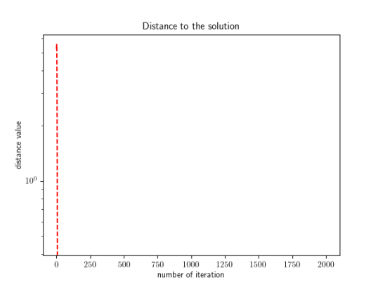
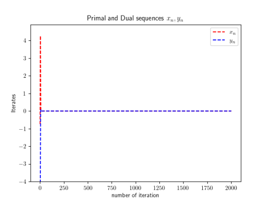
(a)	(b)

Figure 6: Example 7.33. From left to right: distance to the solution; primal-dual iterates.

This is a special case because by the nature of the proximal operator for $f$, which returns zero whenever the iterate is closed enough. That is why primal and dual iterate take zero value just after a few iterations.

Example 7.34.

We consider the Lagrangian

$$\mathcal{L}(x,y)=|x|+|x^{2}-2|+xy-|y|-|y^{2}-2|,$$

which has a similar form as in Example 3.8. It also has one saddle point at $(0,0)$. We run Algorithm 1 for this Lagrangian in two cases: inside and outside the region mentioned in Theorem 4.16. To compute the primal and dual update of Algorithm 1, we use Scipy package in Python to approximate the proximal operator in each step.

Setting:

We set $\tau=0.25,\sigma=0.35,\theta=1$ and we take sharpness constant $\mu=0.9$. The weakly convex modulus $\rho=2$, so the quantity $\frac{\mu}{\max\left\{\frac{1}{2\sigma},\frac{1}{2\tau}\right\}-A}\approx 0.3199,$ where $A=\min\left\{\frac{1-\sqrt{\sigma\tau}\|L\|}{2\tau},\frac{1-\sigma\rho-\theta\sqrt{\sigma\tau}\|L\|}{2\sigma}\right\}\approx 0.00599.$ For the first case, we randomize the starting points $(x_{0},y_{0})\in[-0.3199,0.3199]^{2}$ and for the second case, $[-10,10]^{2}$. We plot the distance of the iterate to the saddle point, both primal and dual iterate in Figure 7 for the first case, and Figure 8 for the second case. Notice the differences in the two figures as the sequences converge to different points from the saddle point in the second case.

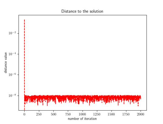
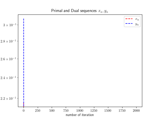
(a)	(b)

Figure 7: Example 7.34; Case $1/2$; From left to right: distance to the solution; primal-dual iterates.

spacing for better view

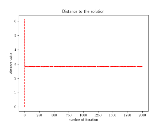
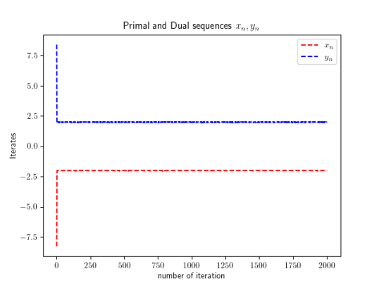
(a)	(b)

Figure 8: Example 7.34; Case $2/2$; From left to right: distance to the solution; primal-dual iterates.

7.2 $\ell_{1}$-regularization

Large scale $\ell_{1}$-regularization

The inf-sharp condition is quite restrictive, as we need to test for Lagrangian. It is much easier to verify sharpness condition (48) for primal objective functions. For example, consider the following $\ell_{1}$ regularization problem in $\mathbb{R}^{n}$

$$\min_{x\in\mathbb{R}^{n}}\|x\|_{1}+\frac{1}{2}\|Ax-b\|^{2},$$ (70)

where $\|x\|_{1}=\sum_{i=1}^{n}|x_{i}|$, $A\in\mathbb{R}^{m\times n}$ is a random transformation matrix and $b\in\mathbb{R}^{m}$ is the noisy data. Our job is to recover the original signal $x^{*}$. Problem (70) is a common reconstruction problem and has been studied extensively in (Combettes and Wajs, 2005; Chambolle and Pock, 2011; Molinari et al., 2021).

Instead of solving problem (70), we modify it into the following

$$\min_{x\in\mathbb{R}^{n}}|\|x\|^{2}-\|x^{*}\|^{2}|+\frac{1}{2}\|Ax-b\|^{2},$$ (71)

which is weakly convex and sharp thanks to the first term (see Bednarczuk et al. (2023b)). Problem (71) has the same meaning as problem (70) as a reconstruction problem from noisy data where one does not know the original signal but its magnitude. We plan to solve both problems (70) and (71) using Algorithm 2 to compare the behavior of the sequence $(x_{n})_{n\in\mathbb{N}}$.

For proximal calculation, the function $\|y-b\|^{2}/2$ is convex and has an explicit form for each update

$$y_{n+1}=\frac{y_{n}-\tau b}{1+\tau}.$$

The function $\|\|x\|^{2}-c|,c>0$ is just a generalization of the one in (Bednarczuk et al., 2023b, Remark 8) so we can have an explicit update with stepsize $2\sigma<1$ as

$$x_{n+1}=\begin{cases}\frac{x_{n}}{1+2\sigma}&\left\|x_{n}\right\|^{2}>\left(1+2\sigma\right)^{2}c,\\ \frac{\sqrt{c}x_{n}}{\left\|x_{n}\right\|}&\left(1-2\sigma\right)^{2}c\leq\left\|x_{n}\right\|^{2}\leq\left(1+2\sigma\right)^{2}c,\\ \frac{x_{n}}{1-2\sigma}&\left\|x_{n}\right\|^{2}<\left(1-2\sigma\right)^{2}c.\end{cases}$$

Setting:

We intend to solve a large-scale sparse problem. Let $n=3000,m=2000$, and $A$ be a random matrix with normal distribution. For $x^{*}\in\mathbb{R}^{n}$, we randomize as a sparse vector with the density of $10\%$ with uniform distribution in $[0,1)$. For noisy data, we set $b=Ax^{*}+\delta$ where we consider two cases for $\delta$: $\delta=0.1$ and $\delta=\|Ax^{*}\|U$ where $U$ is a random vector with uniform distribution in $[-0.1,0.1)$.

Let us set the maximum iterations be $N=5000$ and stepsizes $\sigma=0.1,\tau=\min\{0.99,\frac{1}{\|A\|^{2}\sigma}\},\theta=1$ to ensure that $\|A\|\sqrt{\sigma\tau}<1$. As the starting iterates can affect the algorithm, we test for two cases when $(x_{0},y_{0})$ are zeros vectors and when $x_{0}=E_{0}^{+}x^{*}/\|x^{*}\|$ is close to the solution by the quantity

$$E^{+}_{0}=\frac{\sigma\mu+\sigma\sqrt{\mu^{2}-\frac{\varepsilon_{0}^{2}(\sigma\rho+\sqrt{\sigma\tau}\|A\|)}{\sigma\tau}}}{\sigma\rho+\sqrt{\sigma\tau}\|A\|},$$

where $\mu=0.99,\rho=2,\varepsilon_{0}^{2}=10^{-7}$. This term can be considered as the bounds on the distance in Theorem 6.31. We measure the convergence by calculating $\|x_{n}-x^{*}\|$, and illustrate the performance of Algorithm 2 of two problems (70) and (71) with the same starting points in Figures 9 and 10.

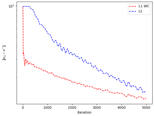
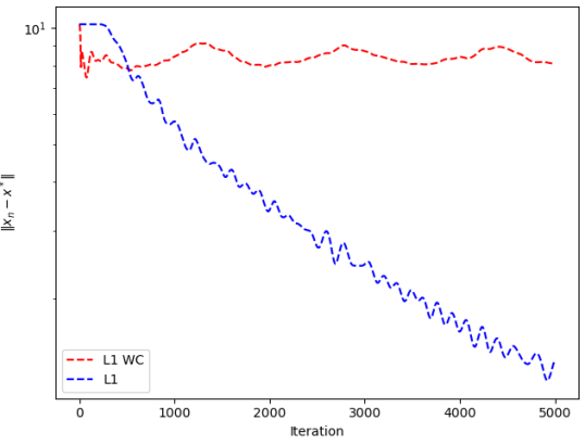
(a)	(b)

Figure 9: Distance to the solution of problem (70) (blue) and (71) (red) with initials: closed to the solution (a), zero (b).

aaaaa

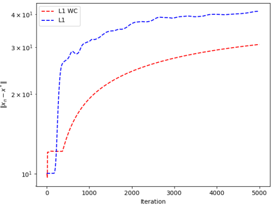
(a)	(b)

Figure 10: Distance to the solution of problem (70) (blue) and (71) (red) for large random noise with initials: closed to solution (a), zero (b).

For the first case with constant noise, Algorithm 2 with close initialization to the solution gives us a better result for weakly convex problem (71) than (70). For zero initialization, $x_{n}$ from (71) tend to be bounded from below by some threshold, while the $x_{n}$ from (70) continue toward the solution. After a particular iteration, Algorithm 1 for convex problem has better results compared to weakly convex problem (71), and continues to decrease to the solution while weakly convex problem stabilizes at some value. We believe that this behavior comes from two factors: we do not put any control on the dual iterate $y_{n}$, and using a proximal subgradient with fixed constant $\rho$ for weakly convex function.

For the second case with larger noise from $\|Ax^{*}\|$, both problems diverge from the solution. As seen in Figure 10, in both initializations, the iterate from weakly convex problem (71) has better error compared to convex problem (70).

Image Deblurring

We use a similar model and comparison in the previous subsection to Image Deblurring.

$$\min_{x}\frac{1}{2}\|Ax-b\|^{2}+\|x\|_{1},$$ (Convex model)

$$\min_{x}|\|x\|^{2}-\|x_{0}\|^{2}|+\frac{1}{2}\|Ax-b\|^{2}.$$ (Weakly Convex model)

Here $x_{0}$ is the original image, the matrix $A$ is a Gaussian blurring matrix, we extract $A$ by applying Gaussian filter with standard deviation $\sigma=4$ to the identity matrix. The quantity $b$ will be the blurred image corrupted with additive noise from normal distribution, $b=Ax+\varepsilon\mathcal{N}(0,1)$ where $\varepsilon=0.01$.

For the setting of the algorithm, we keep the same stepsizes as in the previous example with zeros initialization. We only run the algorithm for $N=1000$ steps. To measure the result, we calculate the peak signal-to-noise ratio (PSNR) with respect to the original image. The higher PSNR implies a better result from the process.

The images are taken from the dataset BSD68 of Github. The images are then rescaled to the value between $[0,1]$ and resized into $256\times 256$. The details for preprocessing steps can be found in Peyré (2011) or (Numerical Tours). We test for several images (number $007,011,013,044$ in the dataset) and show the results in Figure (11). The result shows that the convex model for this application does not work well. The weakly convex model gives improved results compared to the blurred images, as one can recognize the shapes and objects. This is because, in the weakly convex model, we also include the information of the solution $x_{0}$ and the noisy data.

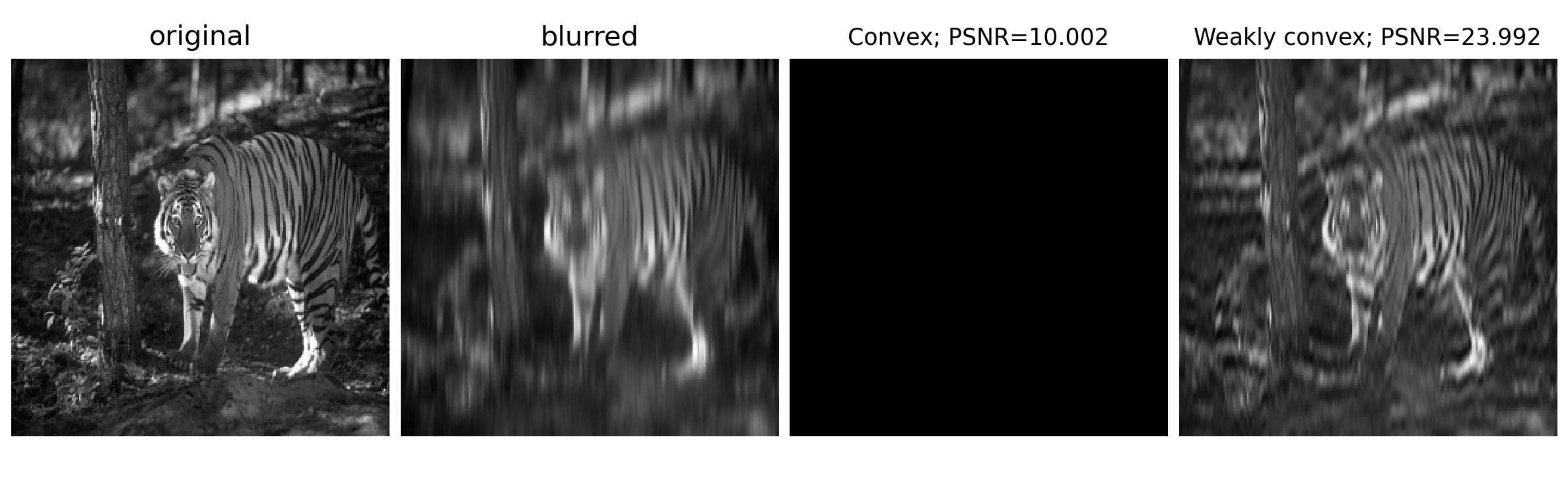
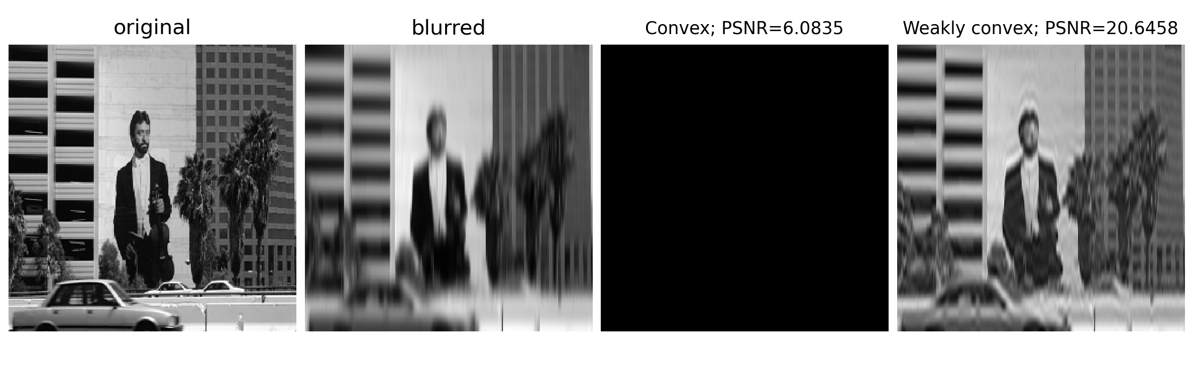
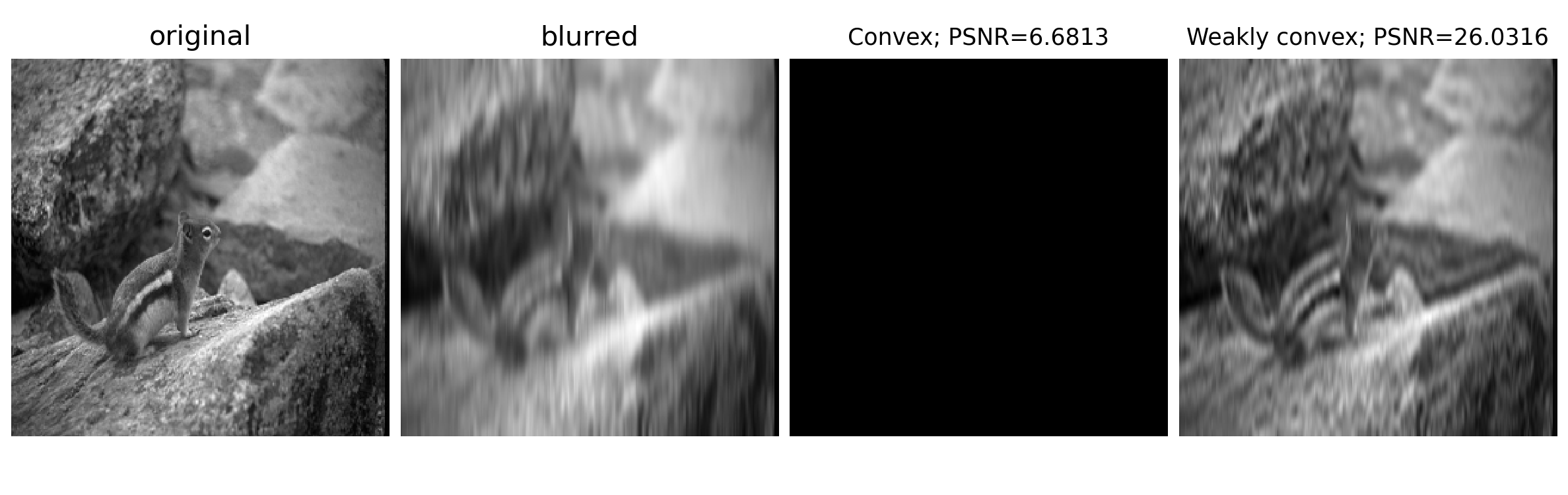
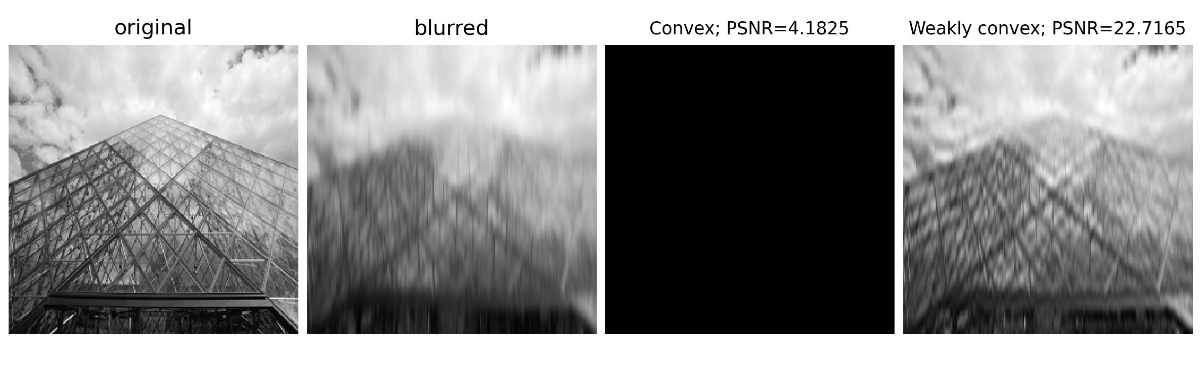
Figure 11: Image Deblurring using convex and weakly convex model.

7.3 Image Denoising with Total Variation

A typical application of the primal-dual algorithm would be Total Variation for image denoising. We consider the following total variation problems and their modification with weakly convex terms,

$$\min_{x\in X}\frac{\lambda}{2}\|x-b\|^{2}+\|\nabla x\|_{1},$$ (Convex model)

$$\min_{x\in X}\lambda|\|x\|^{2}-b|+\|\nabla x\|_{1},$$ (WC-1)

$$\min_{x\in X}|\|x\|^{2}-\|x_{0}\|^{2}|+\frac{\lambda}{2}\|x-b\|^{2}+\|\nabla x\|_{1},$$ (WC-2)

$$\min_{x\in X}\|x-x_{0}\|_{1}+\frac{\lambda}{2}\|x-b\|^{2}+\|\nabla x\|_{1},$$ (WC-3)

$$\min_{x\in X}\|x^{2}-x_{0}^{2}\|_{1}+\frac{\lambda}{2}\|x-b\|^{2}+\|\nabla x\|_{1},$$ (WC-4)

where $x^{2}$ is taken element-wise. All the weakly convex models are sharp except the first model. If we replace $b$ with $\|x_{0}\|^{2}$ in the model (WC-1), then we have no information on the noisy image, which does not make sense. That is why we include $x_{0}$ and $b$ in all other models. We use Algorithm 2 to compare these different models.

The general problem can be written in the form

$$\min_{x\in X}f(x)+\|\nabla x\|_{1},$$

where $\nabla:\mathbb{R}^{n^{2}}\to\mathbb{R}^{2n^{2}}$ is the discrete gradient operator, which can be calculated as $(\nabla x)_{i,j}=((\nabla x)^{1}_{i,j},(\nabla x)^{2}_{i,j}),$ where

$$(\nabla x)^{1}_{i,j}=\begin{cases}u_{i+1,j}-u_{i,j}&i<n,\\ 0&i=n.\end{cases},\qquad(\nabla x)^{2}_{i,j}=\begin{cases}u_{i,j+1}-u_{i,j}&j<n,\\ 0&j=n.\end{cases}$$

We use $g(Lx)=\|\nabla x\|_{1}$ as the composite function. The dual problem will have the form

$$\max_{y\in\mathbb{R}^{2n^{2}}}\min_{x\in\mathbb{R}^{n^{2}}}f(x)-\langle x,\mathrm{div}y\rangle-\delta_{P}(y),$$

where $\delta_{P}(y)$ is the indicator function on the set $P=\{y\in\mathbb{R}^{2n^{2}}:\|y\|_{\infty}\leq 1\}$ with

$$\|y\|_{\infty}=\max_{i,j}|y_{i,j}|,\qquad|y_{i,j}|=\sqrt{(y_{i,j}^{1})^{2}+(y_{i,j}^{2})^{2}}.$$

The function $\mathrm{div}y$ is the discrete divergence operator. All the explicit forms of the gradient and divergence can be found in (Chambolle, 2004; Chambolle and Pock, 2011), as well as an explicit form for the proximal operator. The proximal calculation for $f$ can be made using the explicit form of the previous examples. The proximal for $\ell_{1}$ norm is the softmax function which is available on (Prox-repository).

Setting:

We use the same stepsizes as in the previous example with zeros initialization, and the maximum iteration is $N=2000$. We use (PSNR) to measure the error with respect to the original image. The images will be the same as in the previous example, corrupted with additive noise in the form $b=x_{0}+0.1*\mathcal{N}(0,1)$, where $\mathcal{N}(0,1)$ is the matrix with standard normal distribution. The results are illustrated in Figure 12.

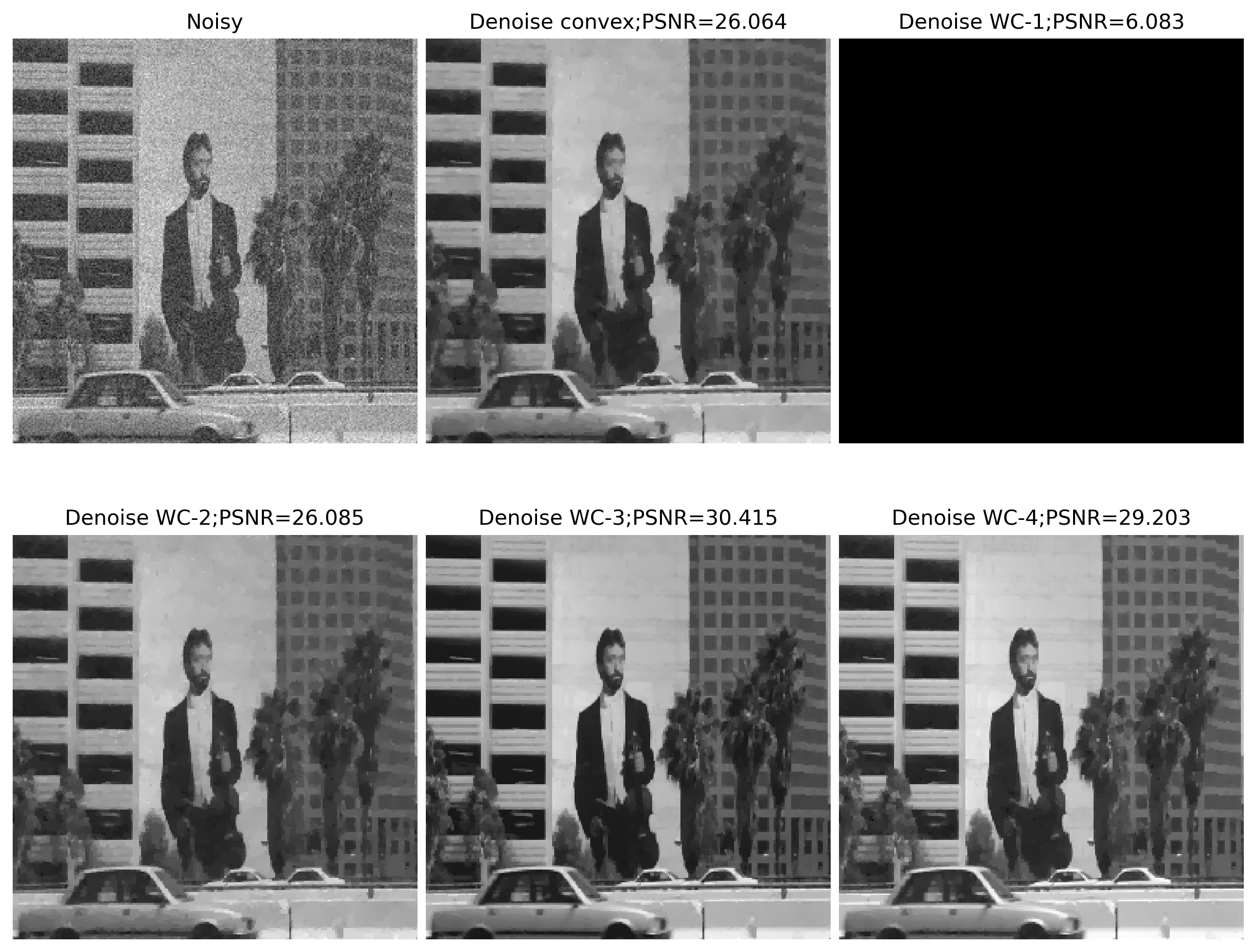
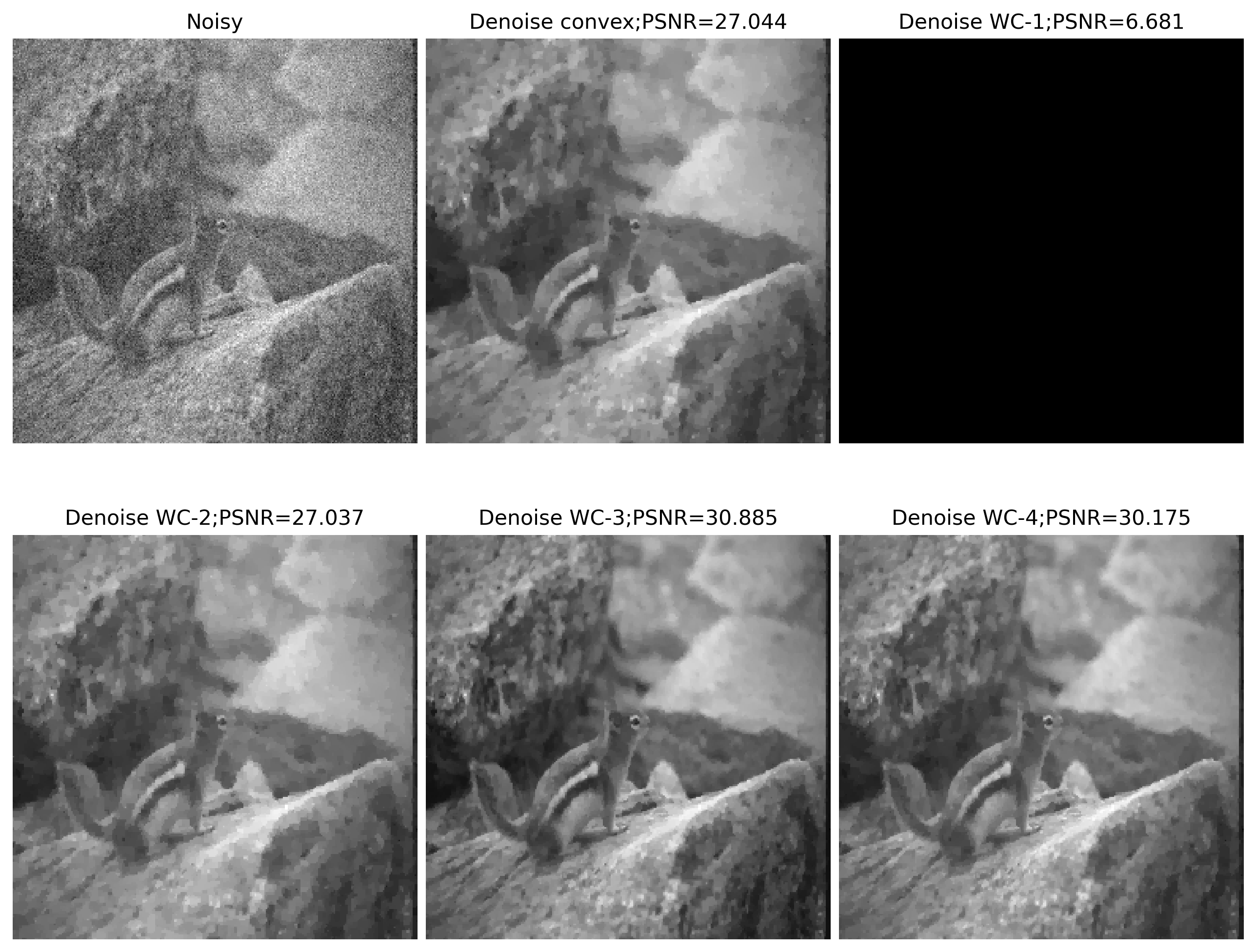
Figure 12: Image Denoising using total variation.

Acknowledgments

This work was funded by the European Union’s Horizon 2020 research and innovation program under the Marie Skłodowska–Curie grant agreement No 861137. This work represents only the authors’ view, and the European Commission is not responsible for any use that may be made of the information it contains.

Supplementary Data

The data used in this work can be found online at Denoising dataset.

References

Applegate et al. (2023)
Applegate, D., Hinder, O.,
Lu, H., Lubin, M., 2023.
Faster first-order primal-dual methods for linear
programming using restarts and sharpness.
Mathematical Programming 201,
133–184.
Atenas et al. (2023)
Atenas, F., Sagastizábal, C.,
Silva, P.J., Solodov, M.,
2023.
A unified analysis of descent sequences in weakly
convex optimization, including convergence rates for bundle methods.
SIAM Journal on Optimization 33,
89–115.
Auslender (1973)
Auslender, A., 1973.
Resolution numerique d’inegalities
variationanelles.
Acad. Sci. A B,
1063–1066.
Bai et al. (2022)
Bai, S., Li, M., Lu, C.,
Zhu, D., Deng, S., 2022.
The equivalence of three types of error bounds for
weakly and approximately convex functions.
Journal of Optimization Theory and Applications
194, 220–245.
Bauschke and Combettes (2017)
Bauschke, H.H., Combettes, P.L.,
2017.
Convex Analysis and Monotone Operator Theory in
Hilbert Spaces.
2nd ed., Springer Publishing
Company, Incorporated.