Synthetic Light Curves and Spectra for the Photospheric Phase of a 3D Stripped-Envelope Supernova Explosion Model

Abstract

We present synthetic light curves and spectra from three-dimensional (3D) Monte Carlo radiative transfer simulations based on a 3D core-collapse supernova explosion model of an ultra-stripped $3.5\,\mathrm{M}_{\odot}$ progenitor. Our calculations predict a fast and faint transient with $\Delta m_{15}\sim 1\texttt{-}2\,\mathrm{mag}$ and peak bolometric luminosity between $-15.3\,\mathrm{mag}$ and $-16.4\,\mathrm{mag}$. Due to a large-scale unipolar asymmetry in the distribution of ${}^{56}\mathrm{Ni}$, there is a pronounced viewing-angle dependence with about $1\,\mathrm{mag}$ difference between the directions of highest and lowest luminosity. The predicted spectra for this rare class of explosions do not yet match any observed counterpart. They are dominated by prominent Mg II lines, but features from O, C, Si, and Ca are also found. In particular, the O I line at ${7}\mathord{,}{774}\,\text{\AA}$ appears as a blended feature together with Mg II emission. Our model is not only faster and fainter than the observed Ib/c supernova population, but also shows a correlation between higher peak luminosity and larger $\Delta m_{15}$ that is not present in observational samples. A possible explanation is that the unusually small ejecta mass of our model accentuates the viewing-angle dependence of the photometry. We suggest that the viewing-angle dependence of the photometry may be used to constrain asymmetries in explosion models of more typical stripped-envelope supernova progenitors in future.

1 Introduction

Most massive stars are destined to end their life in a core-collapse supernova explosion after the exhaustion of the nuclear fuel in their core. Thanks to the advent of large-scale transient surveys, thousands of these events are now detected every year. Samples of well-observed supernovae (e.g., Li et al., 2011; Drout et al., 2011; Müller et al., 2017b; Taddia et al., 2018; Prentice et al., 2019) have already yielded significant insights on the systematics of supernova populations. For some nearby core-collapse supernovae, progenitors have been directly identified using archival images (Van Dyk et al., 2003; Smartt et al., 2009; Smartt, 2015).

Despite the wealth of observational data, our understanding of the explosion mechanism still heavily relies on theory and simulations. Various models for the explosion mechanism have been proposed. Among these, the neutrino-driven mechanism and the magnetorotational mechanism have been most thoroughly explored in simulations (see Janka 2012; Müller 2016, 2020 for reviews). The neutrino-driven mechanism is believed to power the majority of core-collapse supernovae, since this scenario does not require rare progenitors with rapidly rotating cores. In recent years, three-dimensional (3D) simulations have been able to obtain explosions for a wide range of supernova progenitors (e.g., Takiwaki et al., 2012; Melson et al., 2015a; Melson et al., 2015b; Müller, 2015; Müller et al., 2019; Vartanyan et al., 2019; Burrows et al., 2019; Powell & Müller, 2024).

Successful 3D models of neutrino-driven explosions are obviously not enough to confirm the mechanism behind core-collapse supernovae, however. To validate our understanding of the supernova engine, it is essential to compare simulations with observations. There now exist simulations with detailed neutrino transport that extend to sufficiently late times to allow for the calculation of explosion energy, nickel masses, compact remnant masses, kicks, and spins (Müller et al., 2017a; Müller et al., 2019; Nakamura et al., 2019; Bollig et al., 2021; Burrows et al., 2024) as key explosion and remnant properties that can be compared to observationally inferred values. Current simulations predict a plausible range of neutron star kicks, spins, and masses, and can reach the typical explosion energies of Type IIP supernovae from red supergiant progenitors. The predicted explosion energies may, however, still be somewhat lower than observed (Murphy et al., 2019). Bulk explosion properties like the explosion energy and nickel mass are not direct observables, however. They are inferred from the optical light curves and spectra, or other electromagnetic observations outside the optical band. Moreover, a comparison of bulk explosion properties does not constrain the detailed, multi-dimensional explosion dynamics predicted by simulations.

Computing synthetic observables from first-principle simulations is a more ambitious approach to validate or improve theoretical models of the explosion mechanism by pitching them more directly against observational data. For this purpose, explosion models need to be extended from the short engine phase (which lasts for only several seconds) beyond shock breakout on much longer time scales. Relating the multi-dimensional dynamics of the engine phase to observable explosion asymmetries after shock breakout is not straightforward, however. During shock propagation through the stellar envelope, Rayleigh-Taylor (Chevalier, 1976), Kelvin-Helmholtz, and Richtmyer-Meshkov (Richtmyer, 1960) instabilities reshape the spatial distribution of the ejecta compared to the initial asymmetries seeded during the engine phase (Wang & Wheeler, 2008; Müller, 2020).

The outcomes of these mixing instabilities can be observed in supernova spectra and light curves. Historically, mixing instabilities in supernova envelopes gained major prominence due to observations of SN 1987A. Fast iron clumps (Li et al., 1993; Chugai, 1988; Fryxell et al., 1991; Erickson et al., 1988) were unexpectedly observed through spectral lines of high velocity in the first few weeks after the explosion. Asymmetric supernova remnants, such as Cas A and W49B also show evidence of these mixing instabilities, along with global asymmetries formed by either the engine or the progenitor environment (DeLaney et al., 2010; Isensee et al., 2010; Lopez et al., 2013; Grefenstette et al., 2014).

Simulations of mixing instabilities in supernova envelopes have advanced significantly (see Müller 2020 for a review) since the seminal 2D simulations of instabilities and clumping in the aftermath of SN 1987A (Arnett et al., 1989; Müller et al., 1991; Fryxell et al., 1991; Hachisu et al., 1991; Benz & Thielemann, 1990). The most sophisticated modern 3D simulations of mixing instabilities start from 3D engine models with parametrised neutrino transport and tuned engines (Hammer et al., 2010; Wongwathanarat et al., 2013, 2015, 2017), or even from explosion models with multi-group neutrino transport (Chan et al., 2018; Chan & Müller, 2020). So far many of these studies have focused on nearby events or their remnants such as SN 1987A (Hammer et al., 2010; Wongwathanarat et al., 2013, 2015, 2017; Larsson et al., 2013) and Cas A (Wongwathanarat et al., 2017).

In choosing points of reference for a comparison between models and observations, it is important to consider the disparity between engine asymmetries and the observable asymmetries, which limits conclusions on the multi-dimensional dynamics of the engine. For this reason, stripped-envelope supernovae are of particular interest for studying explosion asymmetries. In red and blue supergiant progenitors, strong mixing by the Rayleigh-Taylor instability is caused by the acceleration and subsequent deceleration of the shock at the interface between the helium and hydrogen shell. In stripped-envelope supernovae, the smaller extent or complete lack of the hydrogen envelope implies that initial phase asymmetries are not reshaped as much by strong Rayleigh-Taylor mixing as in explosions of red or blue supergiants.

Among supernova remnants, asymmetries in Cas A (Grefenstette et al., 2014, 2017), the remnant of a Type IIb explosion (Krause et al., 2008) with a partially removed hydrogen envelope, have therefore received particular interest. Among observed transients, Type Ib/c supernovae from hydrogen-free progenitors are particularly promising for leveraging explosion asymmetries as diagnostics of the supernova engine. Observational diagnostics for explosion asymmetries in stripped-envelope supernovae have already been studied extensively. Evidence for non-axisymmetric ejecta in normal Type Ib/c supernovae (as opposed to broad-line Type Ic supernovae), possibly indicative of convective plumes as seed asymmetries in neutrino-driven mechanism, has been found, e.g. by Tanaka et al. (2012); Tanaka et al. (2017) in the form of Q-U loops in the Stokes diagram. The colour evolution in Type Ib/c supernovae has been used as a probe for mixing by correlating the early-time colour evolution of Type Ib/c’s with ^56Ni mixing (Yoon et al., 2019). Line profiles from nebular emission also have a long history as diagnostics for asphericity in Type Ib/c ejecta (Taubenberger et al., 2009; Fang et al., 2022; Milisavljevic et al., 2010).

Aside from Cas A, the investigation of mixing in stripped-envelope supernovae by numerical simulations has been limited. Early 2D simulations (Hachisu et al., 1991, 1994; Kifonidis et al., 2000, 2003) used progenitors with their hydrogen envelopes artificially removed instead of consistently computing the stellar structure and evolution of Type Ib/c supernovae progenitors.

In recent years, interest in stripped-envelope supernovae has increased due to their intimate connection with binary evolution. Most stars are born in multiple star systems and many of these will undergo interactions (Sana et al., 2012). It has been realised, e.g., based on rate arguments, that most Type Ib/c supernovae must originate from progenitors that have lost their hydrogen envelope by mass transfer in such binary systems (Podsiadlowski et al., 1992; Smith et al., 2011; Eldridge et al., 2013). This heightened interest in binary evolution also paves the way for more detailed studies of mixing instabilities in stripped-envelope supernovae and forward modelling of their spectra and light curves based on modern progenitor models (e.g., Claeys et al., 2011; Schneider et al., 2021; Jiang et al., 2021; Tauris et al., 2017) and first-principle supernova simulation to shock breakout. This, however, remains technically demanding; it is still not easy to extend multi-dimensional simulations sufficiently long until the neutrino-driven engine essentially shuts off and the explosion energy is determined. Recently, van Baal et al. (2023) presented a parameterised long-time 3D simulations of a stripped-envelope Type Ib supernova with pre-determined explosion energies and then used this for 3D radiative transfer calculations during the nebular phase. Synthetic light curves and spectra for the photospheric phase based on a self-consistent two-dimensional (2D) explosion model and multi-D Monte Carlo radiative transfer (MCRT) were first presented in our previous work on ultra-stripped supernovae (Maunder et al., 2024).

In this paper, we extend this work to 3D and consider a less extreme progenitor model with higher explosion energy and ejecta mass. We use three-dimensional Monte Carlo radiative transfer to calculate synthetic light curves and spectra based on a first-principle explosion model of a stripped-envelope supernova from Müller et al. (2019). This allows us to investigate the role of ejecta asymmetries on observable light curves and spectra. In particular, we consider the viewing-angle dependence for our 3D model, which shows significant variations in peak luminosity and light curve shape for different observer directions. We compare the model with the population of observed Type Ib/c supernovae to determine the viability of the model and diagnose tensions of current models with observed Type Ib/c supernovae.

2 Progenitor and Explosion Model

In this work, we compute synthetic light curves and spectra for the explosion of a $3.5\,\mathrm{M}_{\odot}$ “ultra-stripped” helium star (Tauris et al., 2015) with an initial metallicity of $\mathrm{Z}=0.02$. The progenitor evolution was simulated using the binary evolution code bec until oxygen burning. In order to reach collapse, the progenitor was then mapped from the binary evolution code bec to the stellar evolution code Kepler (Weaver et al., 1978; Heger et al., 2000).

The star underwent a Case BB common envelope event (Wellstein et al., 2001; Yoon et al., 2010). After the common envelope event, the progenitor was left with a mass of $2.39\,\mathrm{M}_{\odot}$. The composition of the progenitor at the onset of collapse is shown in Figure 1. It has an Fe-Si core of almost $1.5\,\mathrm{M}_{\odot}$, followed by an active oxygen burning shell, an inert O-Ne-Mg shell, a Ne burning shell, and an almost completely burned C shell. Further out, there is a thick He burning shell from $1.8\,\mathrm{M}_{\odot}$ to $2.2\,\mathrm{M}_{\odot}$, followed by a He envelope of about $0.2\,\mathrm{M}_{\odot}$.

The collapse and explosion were simulated in 3D using the relativistic neutrino radiation hydrodynamics code CoCoNuT-FMT (Müller & Janka, 2015). At $1\,\mathrm{s}$ after core bounce, the model was mapped to the Prometheus code (Fryxell et al., 1991; Müller et al., 1991) to follow the evolution beyond shock breakout following the methodology of Müller et al. (2018). A moving grid with an initial radial resolution of $1600$ zones was used for the simulation beyond shock breakout. The angular resolution was $1.6^{\circ}$ on an overset, axis-free Yin-Yang grid (Wongwathanarat et al., 2010).

The model reached an explosion energy of $2.78\times 10^{50}\,\mathrm{erg}$. About $0.8\,\mathrm{M}_{\odot}$ of material is ejected; the innermost $\mathord{\sim}1.6\,\mathrm{M}_{\odot}$ end up in the neutron star (Müller et al., 2019). About $0.023\,\mathrm{M}_{\odot}$ of iron-group material is ejected. The spherically averaged composition of the explosion model at a time of $3424.49\,\mathrm{s}$ is shown in Figure 2.

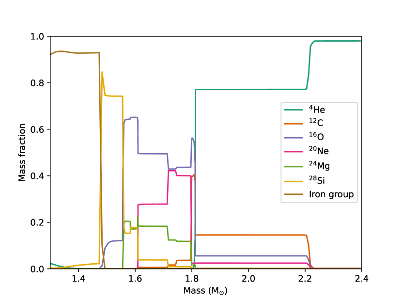
Figure 1: Pre-supernova composition of the progenitor before the onset of core collapse. Only selected elements in the outer part of the iron core and the outer shell are shown. Due to binary mass transfer, the progenitor only has a pre-collapse mass of about $2.4\,\mathrm{M}_{\odot}$.

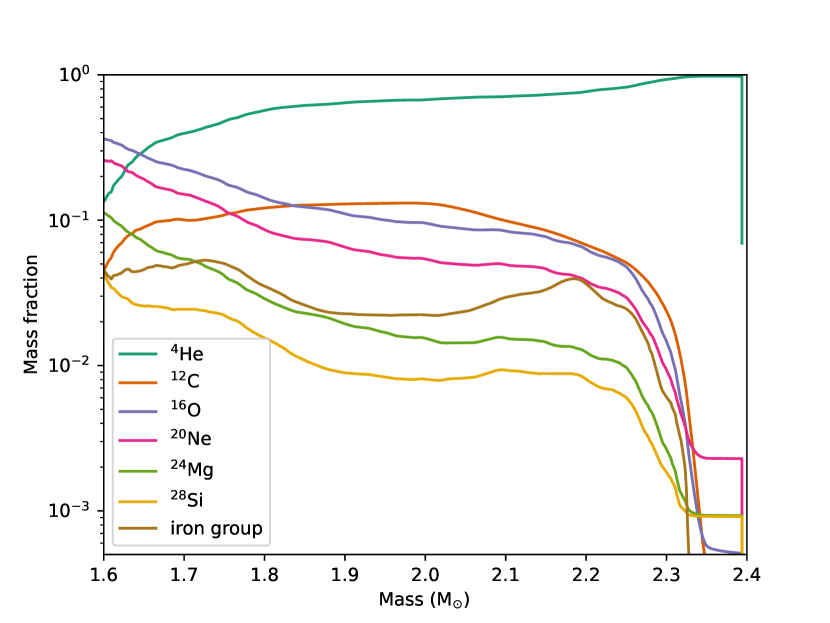
Figure 2: Spherically averaged composition of the 3D explosion model before mapping to the 3D Cartesian grid in Artis . Note that mixing instabilities have modified the initial shell structure of the progenitor.

3 Methods

Synthetic light curves and spectra for the 3D explosion model were generated using the Monte Carlo radiative transfer (MCRT) code Artis (Sim, 2007; Kromer & Sim, 2009; Bulla et al., 2015; Shingles et al., 2020). The code assumes the ejecta are in homologous expansion and that radioactive heating from the decay of ${}^{56}\mathrm{Ni}$ and ${}^{56}\mathrm{Co}$ is the only power source for the transient. The decay chains of ${}^{52}\mathrm{Fe}$ and ${}^{48}\mathrm{Cr}$ are also included in Artis , but their contribution to radioactive heating is negligible for the purpose of this study. Additional power sources such as interactions, magnetised winds, or other central engines are not included.

Artis features a comprehensive set of relevant radiative processes. Our Artis simulations include a detailed set of bound-bound transitions from elements with atomic number $Z=6$ to $30$ (drawn from the CD23 atomic data set, as described by Kromer & Sim 2009, and treated using the Sobolev approximation), as well as bound-free, free-free and electron scattering opacities.

To expedite radiative transfer simulations, Artis applies a grey approximation for the transport in very optically thick cells, whereby packets in zones at high optical depth, defined as having grey optical depth higher than some threshold value, $\tau_{\mathrm{grey}}$ are assumed only to undergo grey scattering and no other interactions with matter (i.e. this has the effect that, at high optical depth, the radiation packets are simply advected with the flow while losing energy due to the expansion; the grey opacity coefficient used is calculated using Equation (8) of Sim et al. 2007).We determined that a high value of $\tau_{\mathrm{grey}}=2500$ is required for convergence.

Note that this study employs the approximate non-LTE treatment of Kromer & Sim (2009), which is expected to be reasonably accurate for the early phase up to and around peak light, but does not include full non-LTE and non-thermal particle excitation/ionisation as required for late-phase spectra. For late-phase spectra, the upgraded non-LTE treatment of Shingles et al. (2020) would be required, but is not included in this study as we focus on the light curves and spectra around peak.

The hydrodynamic explosion model was mapped from the 3D Yin-Yang grid to a 3D Cartesian grid (as required by Artis ) with $100\times 100\times 100$ zones, which is finer than in typical applications of Artis to Type Ia supernovae or kilonovae. For the mapping, we implemented a conservative algorithm that iteratively subdivides the cells of the Yin-Yang grid until the subcells either lie completely within a cell of the Cartesian target grid, or are smaller than a pre-specified fraction of the target cell. The subdivided cells of the original grids are then completely assigned to the target cell that contains their cell centre coordinates. This ensures exact conservation of the total mass and the masses of individual elements and nuclides. Second-order minmod reconstruction is used during the subdivision process to improve the smoothness of the mapped density and mass fraction fields while avoiding overshooting.

After mapping, homologous expansion is assumed. The radiative transfer simulation therefore need not start at the exact time of mapping. In this study we map the hydrodynamical simulation into Artis at $3\mathord{,}424\,\mathrm{s}$ after the onset of the explosion, assume homologous adiabatic expansion until 1 day, and then run the radiative transfer simulations from 1 to 120 days.

Similar to our previous work (Maunder et al., 2024), the treatment of the ejecta composition in the radiative transfer simulation bears careful consideration. The explosion model only tracks 20 nuclear species, namely, ^1H, ^3He, ^12C, ^14N, ^16O, ^20Ne, ^24Mg, ^28Si, ^32S, ^36Ar, ^40Ca, ^44Ti, ^48Cr, ^52Fe, ^54Fe, ^56Ni, ^56Fe, ^60Fe, ^62Ni, along with protons and neutrons. Nuclear burning is only treated with a simple “flashing” treatment based on threshold temperatures (Rampp & Janka, 2000), and nuclear statistical equilibrium (NSE) is assumed above a threshold temperature of $5\,\mathrm{GK}$. Material undergoing freeze-out from NSE will retain its composition at the threshold temperature. This burning treatment is adequate for approximately capturing the overall yields from key burning regimes within reasonable accuracy (e.g., the overall amount of iron group material from Si burning, etc.), but cannot predict the detailed composition of the iron group ejecta self-consistently. The simple burning treatment also ignores potentially important non-$\alpha$ elements (N, Na, etc.) below the iron group. The iron group composition is particularly relevant for the powering of the light curve via the decay of ${}^{56}\mathrm{Ni}$ and ${}^{56}\mathrm{Co}$, but since the isotopic composition is sensitive to the electron fraction in the inner ejecta and hence to details in the neutrino transport, appropriate parameterisations of the composition of the iron-group ejecta can be justified.

Abundances missing from the explosion model are therefore set by modifying the mapped composition based either on typical yields from explosive burning, or on the progenitor composition in unburned regions. The procedure works as follow. When mapping from Prometheus to Artis , protons, neutrons and ^1H are all lumped into ^1H. For the species ^2He through ^36Ar, we directly use the abundances from the explosion model. Abundances of lithium, beryllium, and boron are set to zero. The mass fractions of species from atomic number 20 or above (starting form ^40Ca) are determined by re-scaling their solar abundances to fit the total iron-group mass fraction in the Prometheus simulation in any given grid cell. This procedure ensures that the abundance ratios in the synthesised iron-group material are close to their solar values after the nuclear decays. In iron-rich ejecta, the solar abundances of these species are scaled up proportionally, as one expects them to be made with similar production factors in core-collapse supernovae. The unstable isotope ${}^{56}\mathrm{Co}$ and its stable daughter nucleus ${}^{56}\mathrm{Fe}$ are taken to originate only from the decay of ^56Ni, and their abundances are set according to the elapsed radioactive decays from the start of the explosion. For Ni, we also include ^58Ni separately from ^56Ni according to (scaled) solar abundances.

4 Photometry

4.1 Angled-averaged Emission

We show the bolometric light curves as well as light curves in the U, B, V, R, and I band in Figure 3 in units of magnitudes instead of a linear scale. Note that the U-, B-, and V-band show a bump or plateau after the peak before transitioning to an exponential decline in the tail phase.

The baseline model reaches a peak bolometric luminosity of $8.4\times 10^{41}\,\mathrm{erg}\,\mathrm{s}^{-1}$ after 15 days, putting it distinctly in the faint end of the distribution of observed stripped-envelope supernovae. The UBVRI peak magnitudes (Table 1) range from -16.49 in U band to -15.87 in B band. These are considerably fainter than the average magnitudes in the non-volume limited sample of stripped-envelope supernovae of Drout et al. (2011), who find average R-band peak magnitudes of $-17.0\pm 0.7$ for Ib supernovae and $-17.4\pm 0.4$ for Ic supernovae. The peak magnitudes are, however, quite similar to the average value in the volume-limited LOSS survey (Li et al., 2011) of about $-16.1$ for Ib/c supernovae.

Band	Peak magnitude	Peak time
	(mag)	(days)
U	-16.49	14
B	-15.87	15
V	-16.10	17
R	-16.25	17
I	-16.49	18

Table 1: Peak magnitudes and time of peak for different photometric bands. Data are shown for the baseline model in Figure 3.

Multi-dimensional supernova models are still subject to uncertainties that need to be taken into account in comparisons with observed Ib/c supernovae. Specifically, uncertainties in the explosion energy and the synthesised mass of ${}^{56}\mathrm{Ni}$ will affect the light curve. Because of the computational costs of 3D supernova simulations with multi-group neutrino transport, it is not feasible yet to simulate multiple realisation of the explosions for a particular progenitor with different physics assumptions (e.g., closure relations in the neutrino transport, magnetic fields) that may affect these explosion outcomes. We can, however, still explore some uncertainties by parametrically varying the initial model for the radiative transfer simulation. Most notably, we simulated a model with an artificially increased nickel mass. To increase the nickel mass while maintaining a total mass fraction of one for all cells, we first increased the nickel mass in each zone by a scale factor. After this we took the sum of each zone and used that to renormalise all species within a zone such that the ass fraction in each zone summed correctly to one. For computational convenience, the sensitivity test with increased nickel mass was performed with two runs with a setting of $\tau_{\mathrm{grey}}$=1000. The small convergence error – about 10% in peak bolometric luminosity and much less before and after peak – is significantly smaller than the impact of the increased nickel mass.

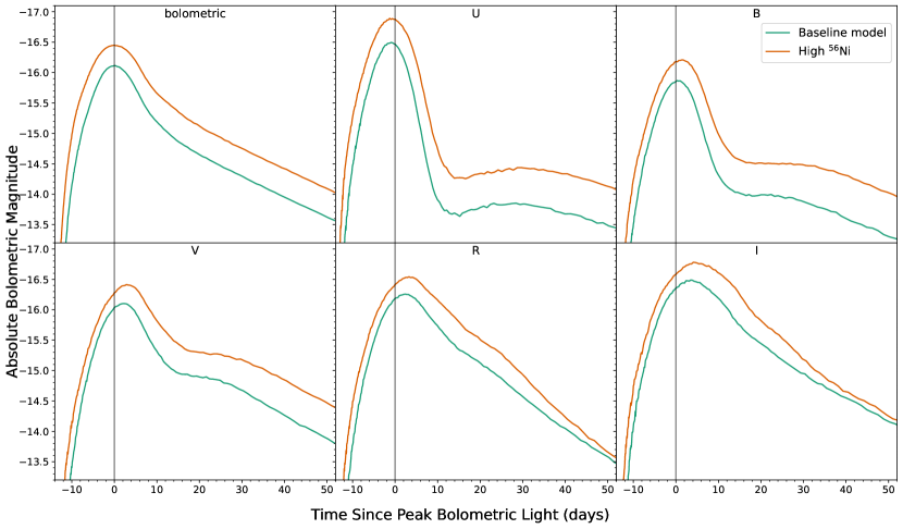
Figure 3: Comparison of the bolometric and UBVRI light curves showing the comparison to the model with increased nickel mass. The purple curve investigated the sensitivity to stronger powering by ^56Ni where we increased the nickel mass by 30%, resulting in an increase in peak brightness of approximately 50%, which is in agreement with what we would expect from Arnett’s rule but does not make our model bright enough to match many more observed events.

We require 30% more nickel mass in order to increase the peak luminosity by $0.34\,\mathrm{mag}$ or $46\,\%$. This is a significant increase in the nickel mass for minimal luminosity increase. This is roughly in accordance with the scaling from Arnett’s rule (Arnett, 1982). The other bands show similar behaviour as the bolometric light curve for the sensitivity tests, with the model with more nickel producing a brighter explosion. Note that the R- and I-band light curves in the model with enhanced nickel mass converge towards the baseline model at late times.

4.2 Viewing-Angle Dependence

In order to investigate potential signatures of explosion asymmetries, we next consider variations in the light curves for different viewing angles. Although the viewing-angle dependence cannot be investigated directly for any observed supernova (except perhaps in a limited fashion in the case of light echos), such a viewing-angle dependence could be studied indirectly by considering variations in the observed supernova population, which we shall address later in Section 6.

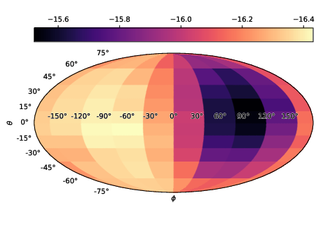
Figure 4: Peak bolometric magnitude for different observer viewing angles. The 100 viewing angle bins are equally spaced in longitude $\phi$ and in the sine of latitude $\theta$, i.e., each bin covers the same solid angle.

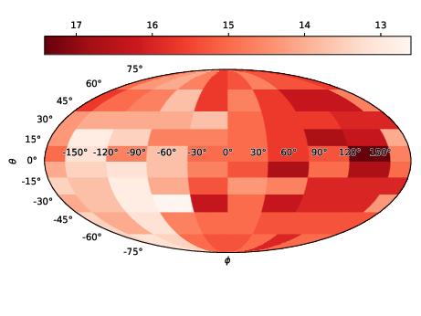
Figure 5: Time of peak bolometric luminosity as a function of viewing angle.

We obtain viewing-angle dependent light curves by binning the emerging photon packets in the baseline radiative transfer simulations into 100 bins of equal solid angle, with uniform spacing in longitude $\phi$ and equal spacing in the cosine of colatitude $\theta$. Figure 4 shows the viewing-angle dependence of the absolute bolometric magnitude at peak light, which will occur at a different time for different viewing angles. The Mollweide projections show a strong dipolar pattern in peak magnitude. The amplitude of the viewing-angle dependence is about $1\,\mathrm{mag}$.

There is also a significant viewing-angle dependence in the time of peak light. Figure 5 shows the time of peak light in days using a similar projection as in Figure 4. Along the viewing angles associated with brighter peak magnitudes, the peak tends to occur earlier. The time of peak varies from 13 to 18 days with a mean of 15 days. The temporal evolution of the brightness variation is shown in Figure 5. The strong viewing-angle dependence is present during the rise and around peak luminosity, but disappears later after peak.

Dipolar variations in peak-magnitude with viewing angle are present, but not perfectly uniform across the entire spectrum. Figure 6 shows the direction-dependent magnitudes at peak light for the bolometric and U, B, V, R, and I bands. The variation in peak magnitude is most pronounced in U band with a variation of $1.24$ and less pronounced at longer wavelengths like the R-band with a variation of 0.79. It is strongest up to and around peak light, and then diminishes later on (Figure 7).

The viewing-angle dependence can be explained by the asymmetric distribution of ${}^{56}\mathrm{Ni}$ in the explosion model. This phenomenon has already been studied in toy models of Type Ia supernovae with parameterised global asymmetries in the ${}^{56}\mathrm{Ni}$ distribution (Sim et al., 2007). If the bulk of ${}^{56}\mathrm{Ni}$ is displaced from the centre of the explosion, photons can more quickly diffuse and escape to the photosphere in the direction aligned with blob because of the lower optical depth from the blob to the photosphere. In modern 3D core-collapse supernova simulations, such large-scale asymmetries in the ${}^{56}\mathrm{Ni}$ distribution emerge naturally from the asymmetries in neutrino-driven convection during the early explosion phase, which usually become dominated by dipole, and sometimes by quadrupole modes around the time of shock revival (Müller et al., 2019). In stripped-envelope supernovae, these initial large-scale asymmetries are well preserved until and beyond shock breakout due to limited additional small- and medium-scale mixing by the Rayleigh-Taylor instability (Chevalier, 1976). Figure 8 shows the distribution of iron-group elements (as a proxy for ${}^{56}\mathrm{Ni}$) around the time of mapping to Artis .

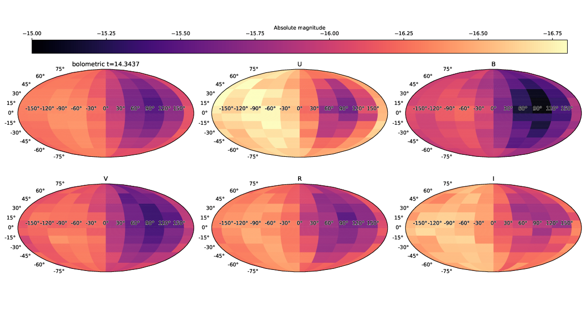
Figure 6: Viewing-angle dependence of the U, B, V, R, I bands at peak bolometric luminosity in addition to the viewing angle-dependence of peak bolometric magntiude.

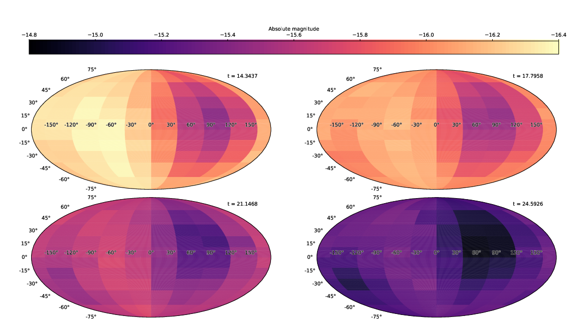
Figure 7: Viewing-angle dependence of the bolometric luminosity for various times from peak light (top left) to about 25 days after the onset of the explosion. Times (in days) are indicated in days next to the luminosity maps.

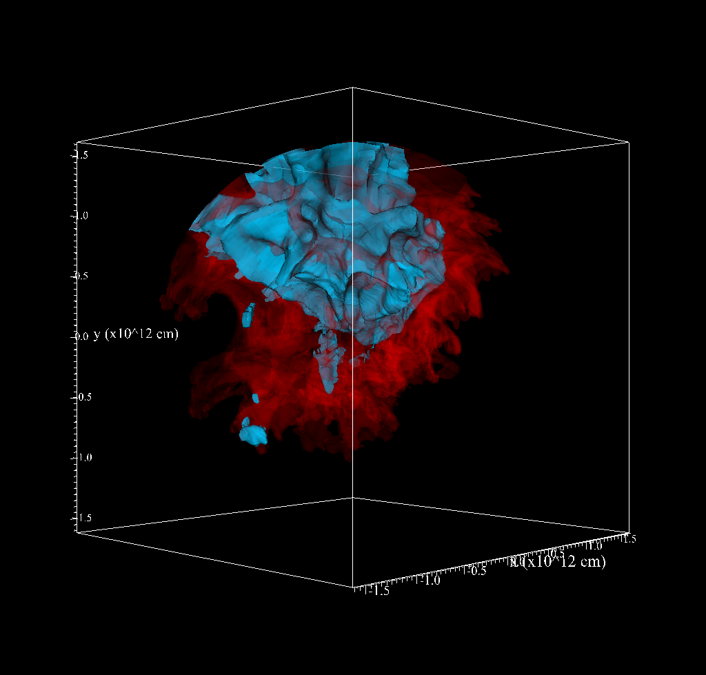
Figure 8: 3D contour plot of the distribution of helium (red) and iron group elements (blue) at time of mapping to Artis . The contour levels for helium and the iron group elements are 0.25 and 0.15, respectively. While the overall ejecta are already somewhat asymmetric, the iron group elements are almost entirely contained within one hemisphere of the ejecta. Note that the structure shown in this plot is still significantly smaller than the entire star. At this time, the stellar surface has expanded to a radius of $9\times 10^{12}\,\mathrm{cm}$.

To illustrate that the viewing-angle dependence is aligned with the asymmetries in the iron-group ejecta, Figure 9 shows the absolute bolometric magnitude and luminosity in solar units for all observer directions $\mathbf{n}^{\prime}$ as a function of the squared distance $|\mathbf{n}-\mathbf{n}^{\prime}|^{2}=1-2\mathbf{n}\cdot\mathbf{n}^{\prime}$ to the centre-of-mass of the iron group elements $\mathbf{n}$. There is a clear correlation between the brightest areas of the photosphere and the (non-central) location of the bulk of the iron-group ejecta. The dependence of the bolometric magnitude on $\cos\theta$ is reasonably tight. The dependence of the bolometric luminosity on $\mathbf{n}\cdot\mathbf{n}^{\prime}$ is fairly linear, so the average bolometric luminosity for a random observer will not be strongly biased away from the mean value. The distribution of observed magnitude will be skewed, however, simply because magnitudes constitute a logarithmic scale. Over about $75\%$ of the sphere, the peak absolute magnitude varies only by about $0.5\,\mathrm{mag}$. The probability to observe the supernova as significantly dimmer than in the brightest direction (e.g., by more than $0.5\,\mathrm{mag}$) is relatively small for a randomly located observer.

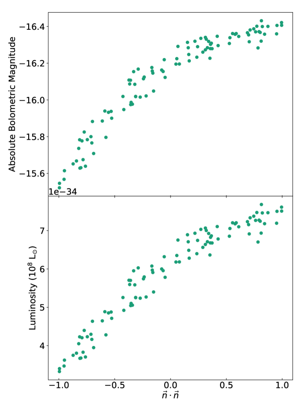
Figure 9: Peak bolometric luminosity (top panel: in magnitudes, bottom panel: on a linear scale) as a function of the angle cosine $\mathbf{n}\cdot\mathbf{n}^{\prime}$ between the observer direction $\mathbf{n}^{\prime}$ and the direction $\mathbf{n}$ of the centre of mass of the iron-group ejecta. The luminosity is highest for observers in the same direction as the iron-group blob. Note the near linearity in luminosity with respect to $\vec{n}\cdot\vec{n}$.

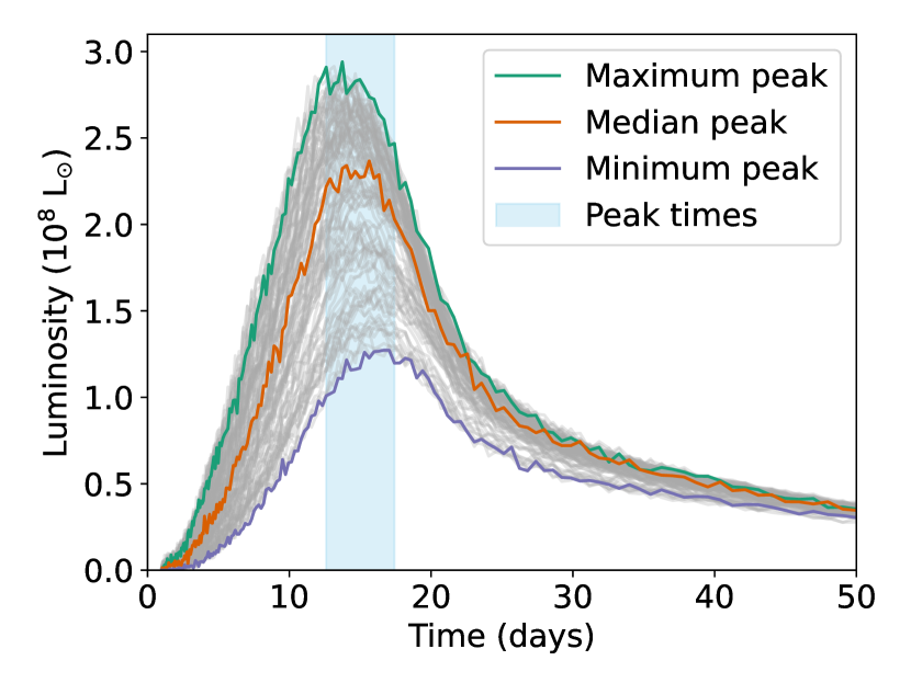
Figure 10: Viewing-angle dependent bolometric light curves for our baseline model. The light curves with the brightest and dimmest peak, and the light curve corresponding to the median of the distribution are shown in green, dark purple, and orange. The light blue region denotes the range of peak times for all different viewing angles.

To illustrate the variations in the light curves for different observer directions, light curves for all 100 viewing angles are shown in grey in Figure 10, together with the light curves corresponding to the minimum, median, and maximum peak brightness. Figure 10 shows that the viewing-angle dependence does not only affect peak luminosity, but also concerns the shape of the light curve. In those directions where the maximum luminosity is higher, the light curve is also more strongly peaked as shown in Figure 10, with a faster evolution of the light curve around maximum brightness. The viewing-angle dependence is most pronounced before and around peak and diminishes during the later phases. In addition, the time of peak also varies slightly; the range of peak epochs is indicated as the light blue region in Figure 10. Such a strong viewing-angle dependence in the light curve has important implications for comparisons to observed stripped-envelope supernovae. This will be discussed in Section 6.

5 Spectroscopy

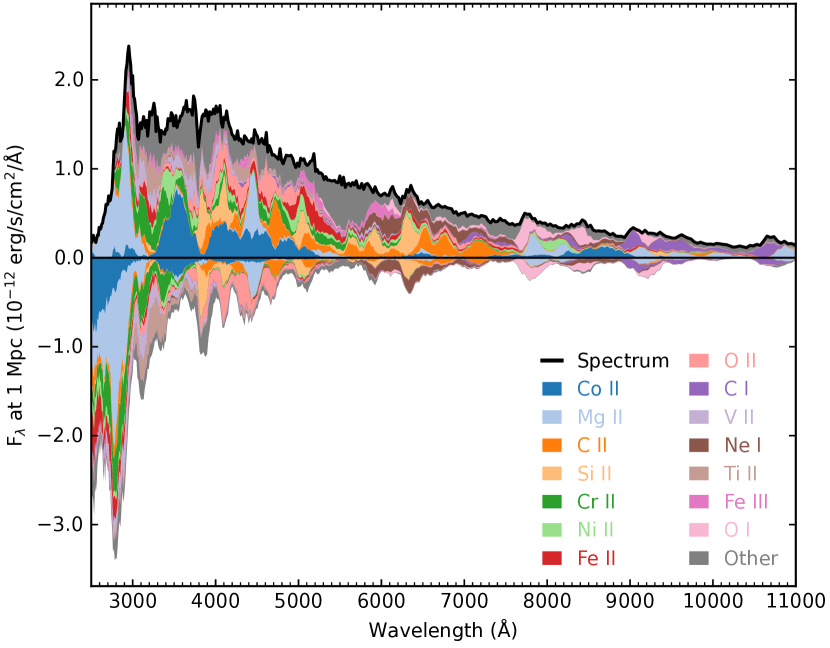
Figure 11: Synthetic spectrum at peak light for our baseline model. Contributions of the 14 most abundant sources of emission (top halves of panels) and absorption (bottom halves) are shown as stacked plot; colours indicate the ion responsible for the last interaction. There is a prominent Mg II feature at 2,800 Å. Overall, this early spectrum shows few identifiable features, similar to the more extreme ultra-stripped supernovae model of Maunder et al. (2024). The spectrum is largely dominated by iron-group elements, Mg II, and some emission from silicon, carbon, oxygen and calcium that only contribute minor features.

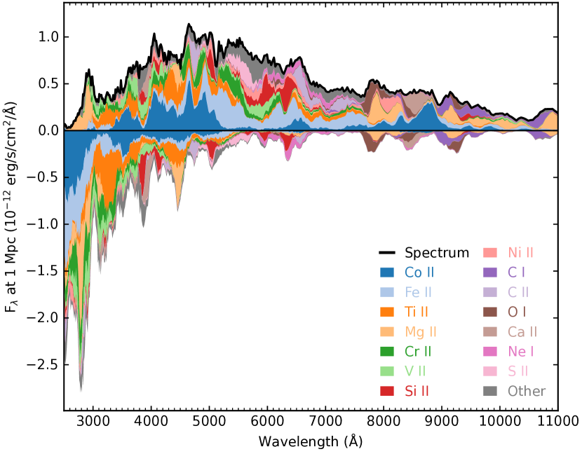
Figure 12: Synthetic spectrum around $6\,\mathrm{d}$ after peak for the baseline model. The prominent Mg II feature at $2\mathord{,}800\,\text{\AA}$ is still present. C II and and Si II features are becoming more clearly visible, and the ${7}\mathord{,}{774}\,\text{\AA}$ O I line appears, blended with a Mg II feature.

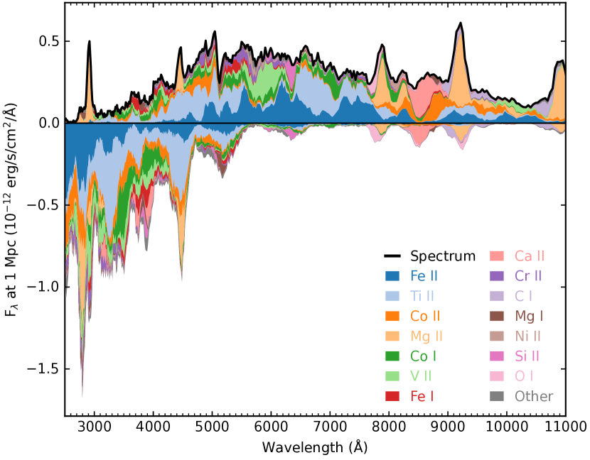
Figure 13: Synthetic spectrum around $12\,\mathrm{d}$ after peak for the baseline model. The Mg II feature at 2800 Å is becoming more prominent again, and more Mg II lines appear in the infrared, as well as the Ca NIR triplet. Identifiable C II and Si II features are no longer present.

Along with photometric information, we also calculate synthetic spectra for our model. Figures 11, 12, and 13 show the emerging angle-averaged spectrum (upper panels) at peak light, $6\,\mathrm{d}$ post-peak and $12\,\mathrm{d}$ post-peak, along with a breakdown into the photon interactions that shape the spectrum. The emerging spectrum in the top halves of panels is broken down into the contributions of the 14 most abundant sources of emission that created the photon packets, with colours indicating the ion or process involved in the last interaction. The bottom halves of the panels show the flux distribution before the last interaction event, which provides an indication for strong scattering or absorption from these wavelength regions.

The most notable feature in the spectra is the prominent Mg II peak at ${2}\mathord{,}{800}\,\text{\AA}$, the same strong line found in the more extreme ultra-stripped supernova model used in our previous work in 2D (Maunder et al., 2024). Aside from that, the spectra do not yet show other clearly identifiable P Cygni lines as one would normally expect from Type Ib/c’s, but there are some features that can be distinctly associated with specific ions. Compared to the 2D model of Maunder et al. (2024), some familiar lines from Type Ib/c spectra do appear in this new model with higher ejecta mass, even though they still differ in detail from observed events. There is another weak Mg II feature in the optical at ${4}\mathord{,}{600}\,\text{\AA}$ which becomes prominent at later times after peak, and some other Mg features in the infrared also become more prominent with time. As found in our previous work, much of the emission comes from iron group elements, namely vanadium, titanium, chromium, iron, and cobalt. More interesting is the presence of C I, C II, Si II and O I lines, which had not appeared as strongly or as early in Maunder et al. (2024), or had not appeared at all.

There is a noticeable ${3}\mathord{,}{858}\,\text{\AA}$ Si II line already at the time of peak. Si II also forms a feature at around ${6}\mathord{,}{300}\,\text{\AA}$ which then disappears by 14 days post-peak. This line is a commonly observed feature in Ic supernovae (Holmbo et al., 2023), although the feature appears only transiently in our model. In the spectrum at 6 days, Si II contributes to several features in the optical and near UV.

The ${7}\mathord{,}{774}\,\text{\AA}$ O I line, which is commonly observed in stripped-envelope supernovae (e.g., Fremling et al., 2018) is already present at peak and remains quite prominent at 6 days after peak, albeit in a blend with a Mg II feature. At late times, the contribution of O I to the blended features is still present, but becomes less prominent. One of the most commonly observed emission features in type Ib/c supernovae, the [O I] ${6}\mathord{,}{300}\,\text{\AA}$ and ${6}\mathord{,}{363}\,\text{\AA}$ lines, are still absent in our models. This is simply due to the fact that these forbidden transition of oxygen are not included in the atomic dataset used in this study (cp. also the discussion of atomic processes relevant to oxygen line formation in van Baal et al. 2023). More generally, the approximate treatment of NLTE in Artis as adopted in this study, will affect the formation of some lines, and is a particularly important limitation for late-time, nebular-phase spectra.

After peak, C II contributes to a narrow feature at around ${4}\mathord{,}{800}\,\text{\AA}$ and a broad feature around ${6}\mathord{,}{600}\,\text{\AA}$-${6}\mathord{,}{800}\,\text{\AA}$, which both disappear by 12 days post-peak. At late times the Ca II triplet around ${8}\mathord{,}{500}\,\text{\AA}$ was a prominent broad feature in our previous work, which is now obscured somewhat by the large Mg II feature around ${9}\mathord{,}{400}\,\text{\AA}$. There is another Mg II peak around ${10}\mathord{,}{900}\,\text{\AA}$. These were not seen to such an extent in our previous work, but the Mg II P Cygni feature at ${2}\mathord{,}{800}\,\text{\AA}$ is less prominent than in the more extremely stripped-model from Maunder et al. (2024). The presence of additional Mg II features is understandable in the light of the higher total mass of Mg in the current model.

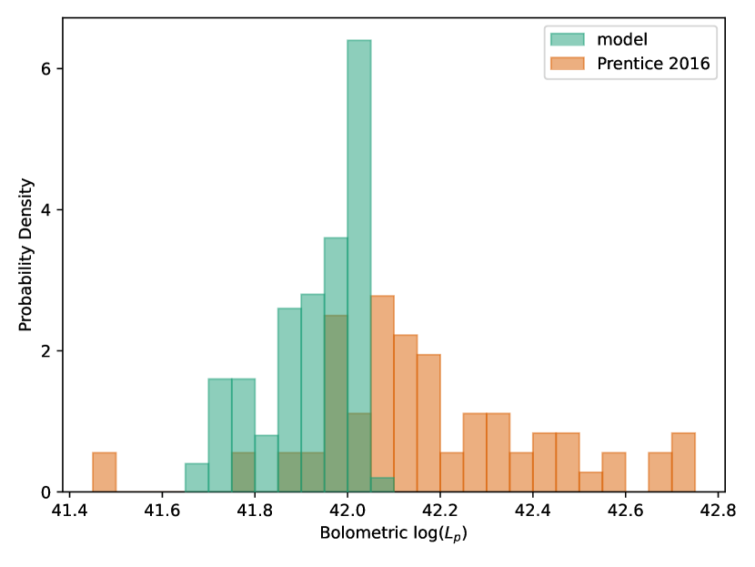
Figure 14: Histogram of peak bolometric magnitude across viewing angles in our model and for the sample of observed Type Ib/c supernovae of Prentice et al. (2016).

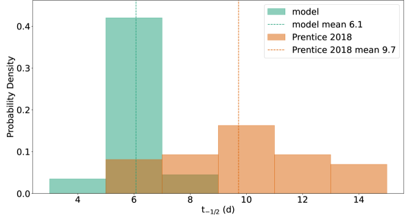
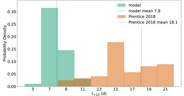
Figure 15: Comparison of the distribution of the half-rise time $t_{-1/2}$ and the half-decay time $t_{+1/2}$ across viewing angles with the observed distribution of $t_{+1/2}$ in the observed Ib/c supernova sample of Prentice et al. (2019).

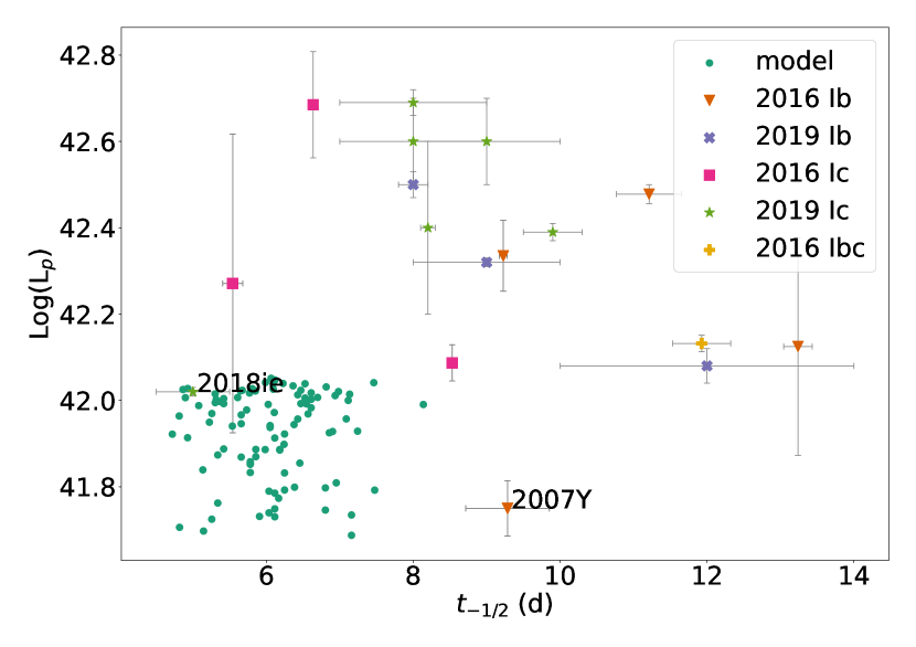
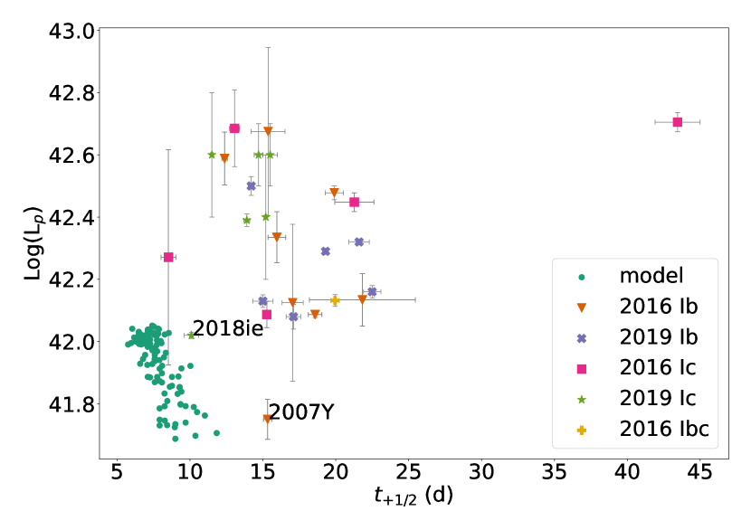
Figure 16: Distribution of peak bolometric luminosity $L_{\mathrm{p}}$ versus half-rise time $t_{-1/2}$ (top panel) and half-decay time $t_{+1/2}$ (bottom panel) across viewing angles for our model, and for the stripped-envelope supernova samples from Prentice et al. (2016, labelled as “2016”) and Prentice et al. (2019, labelled as “2019”). Again the observational samples are broken down into Ib and Ic supernovae , with the addition of some unclear cases (Ibc).

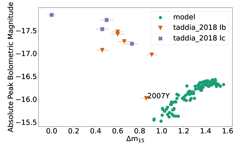
Figure 17: Distribution of peak bolometric magnitude versus $\Delta$m_15,V across viewing angles for our model (circles), and for the stripped-envelope supernova sample of Taddia et al. (2018, symbols with error bars). As in Figure 18, the observed sample is broken down into Ib and Ic supernovae using different colours and symbols.

Figure 18: Distribution of peak absolute V-band magnitude versus $\Delta$m_15,V across viewing angles for our model (circles), and for the stripped-envelope supernova samples (symbols with error bars) of Taddia et al. (2018) and Drout et al. (2011). The observational samples are further broken down into Ib and Ic supernovae using different colours and symbols.

6 Comparison with the Observed Type Ib/c Supernova Population

In comparing to observed stripped-envelope supernovae, we limit ourselves to key features of the photometry since the synthetic spectra still exhibit characteristics very distinct from observed events. Because of the strong viewing-angle dependence of the predicted photometry, it is most appropriate to compare the distribution of photometric properties for different observer directions with the observed population of stripped-envelope supernovae, rather than to focus unduly on matching individual events.

We compare our model to various observational studies of the supernova population, focusing on the Type Ib/c events. The surveys cover a variety of parameters to measure the evolution timescales of the explosions across different optical bands. The surveys from Prentice et al. (2016, 2019) measure the evolution timescales using the time taken to rise from half of the peak brightness to peak, $t_{-1/2}$, and the time taken to decay to half of the peak brightness from time of peak, $t_{+1/2}$. Here we use their bolometric luminosities. The survey in Taddia et al. (2018) provides $\Delta\mathrm{m}_{15}$ values, which measures the change in magnitude over the first 15 days post-peak light. Here we use the V-band and bolometric values. Finally, we use the survey of Drout et al. (2011) who also provide $\Delta\mathrm{m}_{15}$ values and here we use their V-band results. Note that these are not controlled, volume-limited surveys and may hence suffer from a bias towards brighter events.

The comparison to observed transients still places our model at the fast and faint end of the observed stripped-envelope supernova population. Different from the more extreme ultra-stripped supernova model in Maunder et al. (2024), the distribution of brightness across observer directions overlaps with the observed brightness distribution, however. Comparing to the sample of Prentice et al. (2016), the distribution of peak bolometric luminosity overlaps well with the lower half of their observed distribution and reaches almost up to the mean value of their sample thanks to the enhanced brightness in the direction of the iron-group blobs (Figure 14). However, our model evolves significantly faster than most observed transients, as can be seen from histograms of the half-rise $t_{-1/2}$ and half-decay time $t_{+1/2}$ (Figure 15) for the distribution across observer directions in comparison to the samples of Prentice et al. (2016, 2019). We highlight two events that sit within our model’s regime in at least some bands and evolution metrics. Firstly, SN 2007Y is a Type Ic of similar brightness to our event, however, as can be seen in Figures 16-18, the time evolution does not match our model. SN 2007Y is seen to evolve slower both in the rise time and decay time, supported further by the lower $\Delta m_{15}$ in both the V- and R-band. SN 2018ie sits within our distribution of models in the bolometric band half-rise time from Prentice et al. (2016, 2019) and is missing from the sample presented by Drout et al. (2011) and Taddia et al. (2018). This event is also within the range of half-decay times for our models, but these slowly decaying models are dimmer than SN 2018ie. Our model is fainter than the observed sample except for SN 2007Y Our model decays more rapidly than the observed sample aside from SN 2007Y which has a comparable decay time from peak to half-peak.

This mismatch with the observed distribution may simply indicate that the simulated explosion of an ultra-stripped supernova is still too rare an event to be covered by the observed samples due to selection biases. Tauris et al. (2013) estimate the fraction of ultra-stripped Type Ic supernovae to the total supernova rate to be in the range of $10^{-2}-10^{-3}$. Sampling biases in the observed distribution clearly play some role; e.g., there is much less overlap of our predicted viewing-angle dependent brightness distribution with the peak V-band magnitude of Drout et al. (2011); Taddia et al. (2018) and the peak bolometric luminosities of Prentice et al. (2016, 2019). When considering the rise or decay time together with peak luminosity, it is even clearer that our simulation occupies an hitherto unobserved niche in parameter space (Figure 16).

However, the predicted viewing-angle dependence and observed or non-observed correlations of light curve properties may provide a path towards constraining supernova explosion dynamics. Our models show a strong correlation between peak bolometric brightness and $\Delta\mathrm{m}_{15}$, i.e., the decay after peak is faster for higher peak luminosity (Figure 17). The spread in $\Delta\mathrm{m}_{15}$ associated with this correlation amounts to almost $1\,\mathrm{mag}$. To some extent this correlation holds for the peak V-band magnitude as well (figure 18).

The observed population clearly does not not show this correlation between brightness and $\Delta\mathrm{m}_{15}$; there rather is an anti-correlation with brighter events evolving more slowly. This is especially clear when considering bolometric luminosity (Figure 17), where the observed width of the distribution of peak luminosity versus $\Delta\mathrm{m}_{15}$ is quite narrow in the set of Taddia et al. (2018).

This has important implications for the degree of asymmetries in nickel distribution in stripped-envelope supernovae. If the asymmetries in the nickel distribution and the peak luminosity were of similar magnitude as in our model across all stripped-envelope supernovae, the observed distribution of $\Delta\mathrm{m}_{15}$ versus peak luminosity would have to reflect this. Progenitor variations could still give rise to the observed anticorrelation of $\Delta\mathrm{m}_{15}$ versus peak luminosity, but it would be impossible to obtain the narrow distribution of $\Delta\mathrm{m}_{15}$ if there was the same amount of intrinsic scatter of $\Delta\mathrm{m}_{15}$ for individual explosions as in our model. Even if we disregard that the scatter in our model goes in the wrong direction (bigger $\Delta\mathrm{m}_{15}$ for brighter events), the spread in $\Delta\mathrm{m}_{15}$ of $1\,\mathrm{mag}$ in the models is already bigger than that of the observed sample of about $0.5\,\mathrm{mag}$.

Thus, we can clearly conclude that the asymmetries in our model are too large to be representative of generic stripped-envelope supernovae. This does not yet conclusively prove that current 3D supernova explosion models are too asymmetric. In Ib/c supernovae with more massive envelopes of helium and heavier elements, the final distribution of nickel may be less asymmetric, and its impact on the viewing-angle dependence of the light curve may be mitigated by the large optical depth of these outer layers. However, our results demonstrate that the predicted viewing-angle dependence provides a means to constrain explosion asymmetries based on the observed distribution of light curve properties, if either the observed samples can be extended to lower magnitude, or simulations for more massive progenitors become available. Interestingly, the amplitude of the viewing-angle dependence of about $1\,\mathrm{mag}$ at peak is even larger than in the artificial jet-driven explosion models of Rapoport et al. (2012, Figure 2), except perhaps for the U-band, where Rapoport et al. (2012) find a strong direction-dependence during the rise phase. The less pronounced viewing-angle dependence in the jet-driven model could be related to its considerably higher ejecta mass of $10\,\mathrm{M}_{\odot}$. In future, it will be important to investigate whether higher optical depth from the nickel blobs and slower diffusion from the nickel blobs to the photosphere reduce the viewing-angle dependence in less extremely stripped neutrino-driven supernovae.

7 Conclusions

We performed 3D Monte Carlo radiative transfer calculations for a self-consistent explosion model of an ultra-stripped supernovae with a pre-collapse mass of $2.4\,\mathrm{M}_{\odot}$.

The radiative transfer calculations show a relatively faint and rapidly evolving transient with $\Delta m_{15}\sim\texttt{1-2}\,\mathrm{mag}$. Interestingly, we find a considerable viewing-angle dependence in the predicted photometry. The peak magnitude differs by about $1\,\mathrm{mag}$ depending on the observer direction, ranging from $-16.4\,\mathrm{mag}$ down to $-15.3\,\mathrm{mag}$ in bolometric magnitude. The strong viewing-angle dependence is most pronounced up to peak and subsequently decreases. It is caused by the asymmetric distribution of ${}^{56}\mathrm{Ni}$ in the explosion. In directions aligned with the dominant iron-group blob, faster diffusion towards the photosphere results in a significantly enhanced luminosity. The asymmetric distribution of iron-group ejecta also affects the shape of the light curve. Observers in the direction of the iron-group blob would also see more rapidly evolving light curves with a faster rise and decline. This is similar to a phenomenon predicted for toy models of Type Ia supernovae with asymmetric iron distribution (Sim et al., 2007).

Similar to the case of a more extreme ultra-stripped supernova of Maunder et al. (2024), the predicted spectra are unusual for Ib/c supernovae and do not match any observed events. Like in Maunder et al. (2024), the most prominent feature is the Mg II line at ${2}\mathord{,}{800}\,\text{\AA}$. Mg II lines also appear at ${4}\mathord{,}{600}\,\text{\AA}$ in the optical and at ${8}\mathord{,}{000}\,\text{\AA}$, ${9}\mathord{,}{400}\,\text{\AA}$, and ${10}\mathord{,}{900}\,\text{\AA}$ in the infrared during some phases. Different from Maunder et al. (2024), however, lines from other elements emerge as well. The ${7}\mathord{,}{774}\,\text{\AA}$ O I line that is commonly found in Ib/c supernovae appears quite prominently in our model, although it is blended with a Mg II emission feature. The forbidden O I lines at ${6}\mathord{,}{300}\,\text{\AA}$ and ${6}\mathord{,}{363}\,\text{\AA}$ are still absent, as these forbidden transitions are not included in the atomic data set used for this study. We find C emission features around ${4}\mathord{,}{800}\,\text{\AA}$ and ${6}\mathord{,}{600}\,\text{\AA}$-${6}\mathord{,}{800}\,\text{\AA}$ as well as Si II feature around ${3}\mathord{,}{858}\,\text{\AA}$ and ${6}\mathord{,}{300}\,\text{\AA}$ during some epochs. At late times the Ca II NIR (near-infrared) triplet around ${8}\mathord{,}{500}\,\text{\AA}$ appears. The spectral features in our model still differ in detail from observed Ic supernovae – too much to permit a meaningful comparison with individual events – but with the bigger ejecta mass compared to the more extreme ultra-stripped model of Maunder et al. (2024), similarities with observed events are emerging.

Because of the strong viewing-angle dependence of the predicted photometry, it is appropriate to compare the range of predicted photometric properties to the distribution of observed Type Ib/c supernovae rather than to focus unduly on a comparison to single events. Among better observed individual Ib/c supernovae, SN 2007Y is the only one to which our viewing-angle dependent light curves come close to in terms of peak magnitude and rapid evolution. The low luminosity relative to observed Type Ib/c events may still be exaggerated by selection biases. When compared to the sample of Prentice et al. (2016), our predicted viewing-angle dependent bolometric luminosities cover the entire lower half of the observed sample. The comparison to the observed population of stripped-envelope supernovae is more interesting and potentially constraining for supernova explosion models when considering correlation between peak luminosity and the characteristic time scales or post-peak decay rate of the light curves. Our model shows a correlation between higher peak luminosity and a faster decay of the light curve. This correlation between peak bolometric luminosity and $\Delta m_{15}$ is very tight; whereas the correlation between peak V-band magnitude and $\Delta m_{15}$ is less pronounced. Importantly, the observed population of Type Ib/c supernovae does not show such a correlation. There rather appears to be a trend towards slower evolution of brighter events. This implies that the strong viewing-angle dependence in our ultra-stripped model cannot be generic for stripped-envelope supernovae, otherwise these would have to show a much bigger scatter in $\Delta m_{15}$ for a given luminosity.

One possible (and interesting) explanation for this discrepancy would be that current 3D core-collapse supernovae are too asymmetric to be compatible with observed Ib/c supernova photometry. But it is also possible that the strong viewing-angle dependence is a peculiarity due to the low ejecta mass of about $1\,\mathrm{M}_{\odot}$. Similar asymmetries of the ${}^{56}\mathrm{Ni}$ distribution may affect the light curve less if the ${}^{56}\mathrm{Ni}$ is hidden beneath a more massive envelope with higher optical depth. Given that the progenitor considered in this study still represents a rare stellar evolution channel with an unusually small envelope mass, further studies with more typical progenitors are required to determine whether 3D core-collapse supernova explosion models are at odds with the observed photometry of Ib/c supernovae.

Nonetheless, our 3D radiative transfer simulations show a promising avenue towards validating or disproving 3D models of neutrino-driven supernovae of stripped-envelope progenitors. Asymmetries in the ${}^{56}\mathrm{Ni}$ distribution, which are an inherent consequence of the multi-dimensional dynamics seen in modern simulations of neutrino-driven explosions, can leave a significant viewing-angle dependence in the photometry of the observed transient. This viewing-angle dependence would have to be reflected in the distribution of photometric properties across the stripped-envelope supernovae population. The degree and direction of scatter of $\Delta m_{15}$ versus peak luminosity can then serve as a means to constrain explosion asymmetries, even without spectroscopic or polarimetric observations.

Data Availability

The data from our simulations will be made available upon reasonable requests made to the authors.

References

- Arnett (1982) Arnett W. D., 1982, ApJ, 253, 785
- Arnett et al. (1989) Arnett D., Fryxell B., Müller E., 1989, ApJ, 341, L63
- Benz & Thielemann (1990) Benz W., Thielemann F.-K., 1990, ApJ, 348, L17
- Bollig et al. (2021) Bollig R., Yadav N., Kresse D., Janka H.-T., Müller B., Heger A., 2021, ApJ, 915, 28
- Bulla et al. (2015) Bulla M., Sim S. A., Kromer M., 2015, MNRAS, 450, 967
- Burrows et al. (2019) Burrows A., Radice D., Vartanyan D., 2019, MNRAS, 485, 3153
- Burrows et al. (2024) Burrows A., Wang T., Vartanyan D., Coleman M. S. B., 2024, ApJ, 963, 63
- Chan & Müller (2020) Chan C., Müller B., 2020, MNRAS, 496, 2000
- Chan et al. (2018) Chan C., Müller B., Heger A., Pakmor R., Springel V., 2018, ApJ, 852, L19
- Chevalier (1976) Chevalier R. A., 1976, ApJ, 207, 872
- Chugai (1988) Chugai N. N., 1988, Astronomicheskij Tsirkulyar, 1533, 7
- Claeys et al. (2011) Claeys J. S. W., de Mink S. E., Pols O. R., Eldridge J. J., Baes M., 2011, A&A, 528, A131
- DeLaney et al. (2010) DeLaney T., et al., 2010, ApJ, 725, 2038
- Drout et al. (2011) Drout M. R., et al., 2011, ApJ, 741
- Eldridge et al. (2013) Eldridge J. J., Fraser M., Smartt S. J., Maund J. R., Crockett R. M., 2013, MNRAS, 436, 774
- Erickson et al. (1988) Erickson E. F., Haas M. R., Colgan S. W. J., Lord S. D., Burton M. G., Wolf J., Hollenbach D. J., Werner M., 1988, ApJ, 330, L39
- Fang et al. (2022) Fang Q., et al., 2022, ApJ, 928, 151
- Fremling et al. (2018) Fremling C., et al., 2018, A&A, 618, A37
- Fryxell et al. (1991) Fryxell B., Mueller E., Arnett D., 1991, ApJ, 367, 619
- Grefenstette et al. (2014) Grefenstette B. W., et al., 2014, Nature, 506, 339
- Grefenstette et al. (2017) Grefenstette B. W., et al., 2017, ApJ, 834, 19
- Hachisu et al. (1991) Hachisu I., Matsuda T., Nomoto K., Shigeyama T., 1991, ApJ, 368, L27
- Hachisu et al. (1994) Hachisu I., Matsuda T., Nomoto K., Shigeyama T., 1994, A&AS, 104, 341
- Hammer et al. (2010) Hammer N. J., Janka H. T., Müller E., 2010, ApJ, 714, 1371
- Heger et al. (2000) Heger A., Langer N., Woosley S. E., 2000, ApJ, 528, 368
- Holmbo et al. (2023) Holmbo S., et al., 2023, A&A, 675, A83
- Hunter (2007) Hunter J. D., 2007, Computing in Science and Engineering, 9, 90
- Isensee et al. (2010) Isensee K., Rudnick L., DeLaney T., Smith J. D., Rho J., Reach W. T., Kozasa T., Gomez H., 2010, ApJ, 725, 2059
- Janka (2012) Janka H.-T., 2012, Annual Review of Nuclear and Particle Science, 62, 407
- Jiang et al. (2021) Jiang L., Tauris T. M., Chen W.-C., Fuller J., 2021, ApJ, 920, L36
- Kifonidis et al. (2000) Kifonidis K., Plewa T., Janka H. T., Müller E., 2000, ApJ, 531, L123
- Kifonidis et al. (2003) Kifonidis K., Plewa T., Janka H. T., Müller E., 2003, A&A, 408, 621
- Krause et al. (2008) Krause O., Birkmann S. M., Usuda T., Hattori T., Goto M., Rieke G. H., Misselt K. A., 2008, Science, 320, 1195
- Kromer & Sim (2009) Kromer M., Sim S. A., 2009, Monthly Notices of the Royal Astronomical Society, 398, 1809
- Larsson et al. (2013) Larsson J., et al., 2013, ApJ, 768, 89
- Li et al. (1993) Li H., McCray R., Sunyaev R. A., 1993, ApJ, 419, 824
- Li et al. (2011) Li W., et al., 2011, MNRAS, 412, 1441
- Lopez et al. (2013) Lopez L. A., Ramirez-Ruiz E., Castro D., Pearson S., 2013, ApJ, 764, 50
- Maunder et al. (2024) Maunder T., Müller B., Callan F., Sim S., Heger A., 2024, MNRAS, 527, 2185
- Melson et al. (2015a) Melson T., Janka H.-T., Marek A., 2015a, ApJ, 801, L24
- Melson et al. (2015b) Melson T., Janka H.-T., Bollig R., Hanke F., Marek A., Müller B., 2015b, ApJ, 808, L42
- Milisavljevic et al. (2010) Milisavljevic D., Fesen R. A., Gerardy C. L., Kirshner R. P., Challis P., 2010, ApJ, 709, 1343
- Müller (2015) Müller B., 2015, MNRAS, 453, 287
- Müller (2016) Müller B., 2016, Publ. Astron. Soc. Australia, 33, e048
- Müller (2020) Müller B., 2020, Living Reviews in Computational Astrophysics, 6, 3
- Müller & Janka (2015) Müller B., Janka H. T., 2015, MNRAS, 448, 2141
- Müller et al. (1991) Müller E., Fryxell B., Arnett D., 1991, A&A, 251, 505
- Müller et al. (2017a) Müller B., Melson T., Heger A., Janka H.-T., 2017a, MNRAS, 472, 491
- Müller et al. (2017b) Müller T., Prieto J. L., Pejcha O., Clocchiatti A., 2017b, ApJ, 841, 127
- Müller et al. (2018) Müller B., Gay D. W., Heger A., Tauris T. M., Sim S. A., 2018, MNRAS, 479, 3675
- Müller et al. (2019) Müller B., et al., 2019, MNRAS, 484, 3307
- Murphy et al. (2019) Murphy J. W., Mabanta Q., Dolence J. C., 2019, MNRAS, 489, 641
- Nakamura et al. (2019) Nakamura K., Takiwaki T., Kotake K., 2019, PASJ, 71, 98
- Oliphant (2007) Oliphant T. E., 2007, Computing in Science & Engineering, 9, 10
- Podsiadlowski et al. (1992) Podsiadlowski P., Joss P. C., Hsu J. J. L., 1992, ApJ, 391, 246
- Powell & Müller (2024) Powell J., Müller B., 2024, arXiv e-prints, p. arXiv:2406.09691
- Prentice et al. (2016) Prentice S. J., et al., 2016, MNRAS, 458, 2973
- Prentice et al. (2019) Prentice S. J., et al., 2019, Monthly Notices of the Royal Astronomical Society, 485, 1559
- Rampp & Janka (2000) Rampp M., Janka H.-T., 2000, ApJ, 539, L33
- Rapoport et al. (2012) Rapoport S., Sim S. A., Maeda K., Tanaka M., Kromer M., Schmidt B. P., Nomoto K., 2012, ApJ, 759, 38
- Richtmyer (1960) Richtmyer R. D., 1960, Communications on Pure and Applied Mathematics, 13, 297
- Sana et al. (2012) Sana H., et al., 2012, Science, 337, 444
- Schneider et al. (2021) Schneider F. R. N., Podsiadlowski P., Müller B., 2021, A&A, 645, A5
- Shingles et al. (2020) Shingles L. J., et al., 2020, MNRAS, 492, 2029
- Shingles et al. (2024) Shingles L. J., Collins C. E., Holas A., Callan F., Sim S., 2024, artistools, doi:10.5281/zenodo.13752138, https://doi.org/10.5281/zenodo.13752138
- Sim (2007) Sim S. A., 2007, MNRAS, 375, 154
- Sim et al. (2007) Sim S. A., Sauer D. N., Röpke F. K., Hillebrandt W., 2007, MNRAS, 378, 2
- Smartt (2015) Smartt S. J., 2015, Publ. Astron. Soc. Australia, 32, e016
- Smartt et al. (2009) Smartt S. J., Eldridge J. J., Crockett R. M., Maund J. R., 2009, MNRAS, 395, 1409
- Smith et al. (2011) Smith N., Li W., Filippenko A. V., Chornock R., 2011, MNRAS, 412, 1522
- Taddia et al. (2018) Taddia F., et al., 2018, Astronomy and Astrophysics, 609
- Takiwaki et al. (2012) Takiwaki T., Kotake K., Suwa Y., 2012, ApJ, 749, 98
- Tanaka et al. (2012) Tanaka M., et al., 2012, ApJ, 754, 63
- Tanaka et al. (2017) Tanaka M., Maeda K., Mazzali P. A., Kawabata K. S., Nomoto K., 2017, ApJ, 837, 105
- Taubenberger et al. (2009) Taubenberger S., et al., 2009, MNRAS, 397, 677
- Tauris et al. (2013) Tauris T. M., Langer N., Moriya T. J., Podsiadlowski P., Yoon S. C., Blinnikov S. I., 2013, ApJ, 778, 23
- Tauris et al. (2015) Tauris T. M., Langer N., Podsiadlowski P., 2015, MNRAS, 451, 2123
- Tauris et al. (2017) Tauris T. M., et al., 2017, ApJ, 846, 170
- Van Dyk et al. (2003) Van Dyk S. D., Li W., Filippenko A. V., 2003, PASP, 115, 1
- Vartanyan et al. (2019) Vartanyan D., Burrows A., Radice D., Skinner M. A., Dolence J., 2019, MNRAS, 482, 351
- Wang & Wheeler (2008) Wang L., Wheeler J. C., 2008, Annual Review of Astronomy and Astrophysics, 46, 433
- Weaver et al. (1978) Weaver T. A., Zimmerman G. B., Woosley S. E., 1978, ApJ, 225, 1021
- Wellstein et al. (2001) Wellstein S., Langer N., Braun H., 2001, A&A, 369, 939
- Wongwathanarat et al. (2010) Wongwathanarat A., Hammer N. J., Müller E., 2010, A&A, 514, A48
- Wongwathanarat et al. (2013) Wongwathanarat A., Janka H. T., Müller E., 2013, A&A, 552, A126
- Wongwathanarat et al. (2015) Wongwathanarat A., Müller E., Janka H. T., 2015, A&A, 577, A48
- Wongwathanarat et al. (2017) Wongwathanarat A., Janka H.-T., Müller E., Pllumbi E., Wanajo S., 2017, ApJ, 842, 13
- Yoon et al. (2010) Yoon S.-C., Woosley S. E., Langer N., 2010, The Astrophysical Journal, 725, 940
- Yoon et al. (2019) Yoon S.-C., Chun W., Tolstov A., Blinnikov S., Dessart L., 2019, ApJ, 872, 174
- van Baal et al. (2023) van Baal B., Jerkstrand A., Wongwathanarat A., Janka T. H., 2023, preprint, arXiv:2305.08933