Projection-based Reduced Order Modelling for Unsteady Parametrized Optimal Control Problems in 3D Cardiovascular Flows

Abstract

This paper presents a projection-based reduced order modelling (ROM) framework for unsteady parametrized optimal control problems (OCP_(μ)s) arising from cardiovascular (CV) applications. In real-life scenarios, accurately defining outflow boundary conditions in patient-specific models poses significant challenges due to complex vascular morphologies, physiological conditions, and high computational demands. These challenges make it difficult to compute realistic and reliable CV hemodynamics by incorporating clinical data such as 4D magnetic resonance imaging. To address these challenges, we focus on controlling the outflow boundary conditions to optimize CV flow dynamics and minimize the discrepancy between target and computed flow velocity profiles. The fluid flow is governed by unsteady Navier–Stokes equations with physical parametric dependence, i.e. the Reynolds number. Numerical solutions of OCP_(μ)s require substantial computational resources, highlighting the need for robust and efficient ROMs to perform real-time and many-query simulations. Here, we aim at investigating the performance of a projection-based reduction technique that relies on the offline-online paradigm, enabling significant computational cost savings. The Galerkin finite element method is used to compute the high-fidelity solutions in the offline phase. We implemented a nested-proper orthogonal decomposition (nested-POD) for fast simulation of OCP_(μ)s that encompasses two stages: temporal compression for reducing dimensionality in time, followed by parametric-space compression on the precomputed POD modes. We tested the efficacy of the methodology on vascular models, namely an idealized bifurcation geometry and a patient-specific coronary artery bypass graft, incorporating stress control at the outflow boundary, observing consistent speed-up with respect to high-fidelity strategies.

1 Introduction

In recent years, the integration of well-established computational methodologies with optimization techniques has gained popularity in the realm of computational flow control and optimization [1, 2]. Many advances have been made in the analysis of optimal control problems (OCPs), especially for viscous, incompressible flows governed by partial differential equations (PDEs) with applications in engineering, environmental, and biomedical fields [3, 4, 5, 6, 7]. These advances rely on developing models and computational algorithms to solve them. OCPs strive to identify control inputs that effectively uphold the extrema of an objective function while ensuring all constraints are met, and have been widely used in engineering to optimize the performance of complex systems. The analysis of OCPs governed by PDEs is based on the theory developed by J. L. Lions [8, 9]. Parametrized optimal control problems (OCP_(μ)s) represent a broader class of optimization problems characterized by a set of parameters [10, 11, 12, 13, 14], wherein the parameters, denoted by $\bm{\mu}$ $\in\mathcal{D}$, characterize some physical and/or geometrical properties of the system. The control may act as a forcing term, a boundary condition, an initial condition, or even as a coefficient in the equation. These research studies have developed advanced control strategies to provide flexibility, adaptability, and versatility, which have significant implications for various engineering applications. In particular, the works [15, 16] offer an advanced perspective for comprehending system behaviour and control strategies in the realm of biomedical applications.

Over the decades, mathematical modelling and scientific computing have proven to be vital tools in advancing our understanding of the complex physiology of cardiovascular (CV) systems and their underlying causes. The relationships between hemodynamics and CV diseases are complex and multifaceted, as discussed in [17, 18, 19, 20]. The challenges associated with CV modelling are mainly due to: $(i)$ high computational costs; $(ii)$ complex vascular morphologies and their meshing; and $(iii)$ the setting of accurate boundary conditions, which is vital for blood flow analysis [21, 22, 23, 24, 25]. The studies [22, 24, 26] underscore the significance of outflow boundary conditions in the computational modelling of patient-specific models, including the consideration of numerical backflow. Hence, it is imperative to account for many different factors when developing numerical techniques to provide quantitative insights into blood flow dynamics within vascular regions. In this framework, coronary artery bypass grafting (CABG) is a widely adopted surgical technique used globally to treat patients with coronary artery diseases [27, 28, 29]. This technique involves creating new pathways around blocked or narrowed coronary arteries to restore proper blood flow to the heart muscle. Numerous computational studies have been performed for CABG models [30, 31, 32, 33], where the outflow boundary condition is typically set as a “do-nothing" (i.e., homogeneous Neumann) condition. However, incorporating the outflow boundary condition as a controlled parameter in CV modelling entails applying principles from OCPs to optimize blood flow dynamics. In [34, 35], the outflow boundary is estimated as a controlled parameter for a two-dimensional bifurcation vascular model and for an aortic model, respectively, using the OCP framework to optimize physiological simulations for steady Stokes flow. The intricate connection between vessel geometries and hemodynamics are vital for the analysis, and can be better understood through advanced computational methods, but this requires high computational cost. Such task becomes even more challenging if real-time solutions of the OCP_(μ)s are needed, spanning across the whole parameter domain $\mathcal{D}\subset\mathbb{R}^{P}$ with $P\geq 1$, known as the many-query context.

To achieve this objective, we employ the reduction approaches for OCP_(μ)s governed by PDE_(μ)s in which the high-fidelity numerical system of dimension, say $\mathcal{N}$, is replaced by constructing low-dimensional problem-specific approximation spaces $(N^{rd}\ll\mathcal{N})$, discussed in [36, 37, 38, 39, 40]. This framework adheres to the offline-online paradigm, where the high-fidelity solution manifold is computed using the Galerkin Finite Element (FE) method (or other classical numerical approaches) during the offline phase, requiring considerable computational resources to properly capture physical and/or geometric variability. On the other hand, the online phase leverages the precomputed quantities to generate a low-dimensional approximation manifold which is more efficient to query. Enhancing the computational efficiency, these reduction methodologies have gained considerable attention, and researchers have delved into various model reduction strategies, including certified reduced basis [41, 42], proper orthogonal decomposition (POD) [37, 43], and non-intrusive approaches[44, 45, 46]. These approaches are often applied to engineering and CV applications involving PDE_(μ)s [47, 48, 49, 50, 39, 51, 52, 53, 54], to provide very efficient solutions. However, projection-based intrusive ROMs, exploiting the knowledge of the physical model, offer significantly improved reliability and accuracy in computing the reduced order solutions. These methods project the high-dimensional system onto a lower-dimensional subspace, typically spanned by dominant modes computed from the high-fidelity solutions; they effectively capture the essential properties of the system’s dynamics while significantly reducing the computational complexity of the online phase. In [55], such intrusive strategy has been used to investigate potential sources of pressure instabilities, exploiting the supremizer stabilization to prevent spurious pressure modes in the POD approximation of parametrized flows. By leveraging these techniques, the authors have significantly improved the efficiency and accuracy of their computational analyses of vascular models, as detailed in [51]. In [56], OCP_(μ)s using classical POD techniques has been used to understand the flow characteristics of a two-dimensional bifurcation model governed by the unsteady Stokes equations. The authors of [57] introduced an intrusive reduction technique for computing hemodynamics in CABGs using the Navier–Stokes (N–S) equations, which employs an advanced POD technique to extract dominant flow modes from high-fidelity solutions.

This paper presents a novel approach to reducing the computational complexity of simulating spatio-temporal flow in complex three-dimensional vascular models formulated as parametrized OCPs. We implemented a projection-based reduction strategy for OCP_(μ), effectively addressing the nonlinearities inherent in the unsteady N–S equations. The primary goal of the proposed methodology is to optimize blood flow dynamics by estimating outflow boundary conditions, treated as control variables, that minimize variations of the flow fields from a target velocity profile. This entails formulating parametrized OCPs that integrate the unsteady N–S equations along with boundary conditions, as well as assessing the impact of various physical parameters governing the system. Given the substantial computational costs and iterative procedures involved in solving the optimal control problems, to address the computational challenges associated with solving these complex models, we strategically leverage dimensional reduction techniques, particularly the nested-POD, to enhance the computational efficiency while keeping a high level of accuracy. The structure of this paper is as follows: Section 2 introduces the framework of OCP_(μ)s and discusses the Lagrangian formulation. Section 3 discusses the numerical methods employed, beginning with Galerkin FE formulation in Section 3.1, which is pivotal for computing high-fidelity solutions, as well as presenting a projection-based ROM for OCP_(μ) in Section 3.2. Moreover, Section 4 presents a detailed analysis of the numerical simulations, focusing on the comparison between high-fidelity and reduced-order approximations, and examining the flow field characteristics and unsteady flow dynamics within vascular models. Finally, the conclusions are outlined in Section 5.

2 Mathematical Modelling

This section presents a mathematical modelling framework for OCP_(μ)s, focusing on determining the optimal control strategy for dynamical systems. These problems comprise multiple parts: state equations governing the fluid flow, a cost functional to be minimized, dependency on the physical properties, and a control variable that influences fluid flow. The Lagrangian formulation exploits the so-called Lagrange multipliers to incorporate constraints into the optimization problem, yielding the necessary conditions for optimality.

2.1 Parametrized OCPs for Unsteady Navier-Stokes Equations

We aim at solving OCPs with parametric dependence, in which optimal solutions depend on parameters $\bm{\mu}\in\mathcal{D}$. The abstract formulation of OCP_(μ)s is expressed as [2, 58]:

$$\begin{gathered}\textit{given}\,\bm{\mu}\in\mathcal{D},\,\textit{find the optimal control}\,\,\bm{u}\left(\bm{x},t;\bm{\mu}\right)\,\textit{and the state variable}\,\,\bm{y}\left(\bm{x},t;\bm{\mu}\right)\\ \textit{s.t.\ cost functional}\,\,\mathcal{J}\left(\bm{y}\left(\bm{x},t;\bm{\mu}\right),\bm{u}\left(\bm{x},t;\bm{\mu}\right);t;\bm{\mu}\right)\,\textit{is minimized subject to}\,\,\mathcal{E}\left(\bm{y}\left(\bm{x},t;\bm{\mu}\right),\bm{u}\left(\bm{x},t;\bm{\mu}\right);t;\bm{\mu}\right)=0.\end{gathered}$$ (1)

In problem (1), $\bm{\mu}\in\mathcal{D}\subset\mathbb{R}^{P}$ represents the physical parameter vector of the system, with dimension $P\geq 1.$ The state equation $\displaystyle\mathcal{E}\left(\bm{y}\left(\bm{x},t;\bm{\mu}\right),\bm{u}\left(\bm{x},t;\bm{\mu}\right);t;\bm{\mu}\right)$ describes how the state solution $\bm{y}\left(\bm{x},t;\bm{\mu}\right)\in\mathbf{Y}$ evolves with space and time under the influence of the control $\bm{u}\left(\bm{x},t;\bm{\mu}\right)\in\mathcal{U}.$ The control may correspond to a forcing term, boundary condition, or initial condition, with the spaces $\mathcal{U}$ and $\mathbf{Y}$ representing the control space and state space, respectively. In this study, the dynamical system is a CV system, which is governed by the unsteady N–S equations with some specified initial and/or boundary conditions. In these optimization problems, the observation of the state variable is often represented by a linear mapping, $z\left(\bm{y}\left(\bm{x},t;\bm{\mu}\right)\right)=\bm{C}\bm{y}\left(\bm{x},t;\bm{\mu}\right),$ where $\bm{C}$ is a suitable operator. The cost functional $\displaystyle\mathcal{J}\left(\bm{y}\left(\bm{x},t;\bm{\mu}\right),\bm{u}\left(\bm{x},t;\bm{\mu}\right);t;\bm{\mu}\right)$ is defined based on the observation, and potentially a desired profile, within the observation space $\left(\mathcal{Z}\supseteq\mathbf{Y}\right)$ associated with the dynamical system.

Let us consider a spatio-temporal domain $\Omega\times\left(0,T\right)$, where $\Omega\subset\mathbb{R}^{n_{\mathrm{sd}}}$, with $n_{\mathrm{sd}}=2,3$ representing the spatial dimension, and $T\geq 0$ is the final time. The boundary of the spatial domain $\Omega$ can be expressed as a disjoint union of the boundaries, i.e. $\Gamma=\Gamma_{\mathrm{w}}\cup\Gamma_{\mathrm{in}}\cup\Gamma_{\mathrm{out}}$, where $\Gamma_{\mathrm{w}}$, $\Gamma_{\mathrm{in}}$, and $\Gamma_{\mathrm{out}}$, respectively, represent the wall, inlet, and outflow boundaries of the computational models. A rigid wall assumption is considered for the computation, and the blood is modelled as an incompressible Newtonian fluid governed by the unsteady N–S equations.

For any given $\bm{\mu}\in\mathcal{D}$, the OCP_(μ)s in Problem (1) can be stated as:

$$\begin{gathered}\displaystyle\min_{\bm{v}\in\mathcal{V},\bm{u}\in\mathcal{U}}\mathcal{J}\left(\bm{v}\left(t;\bm{\mu}\right),\bm{u}\left(t;\bm{\mu}\right);t;\bm{\mu}\right),\\[5.69046pt] \text{where}\quad\mathcal{J}\left(\bm{v}\left(t;\bm{\mu}\right),\bm{u}\left(t;\bm{\mu}\right);t;\bm{\mu}\right)\doteq\frac{1}{2}\int_{0}^{T}\int_{\Omega}m_{d}\left(\bm{v}\left(t;\bm{\mu}\right),\bm{v}_{d};t;\bm{\mu}\right)\,dt+\frac{\alpha}{2}\int_{0}^{T}\int_{\Omega}\mathcal{R}\left(\bm{u}\left(t;\bm{\mu}\right);t;\bm{\mu}\right)\,dt.\end{gathered}$$ (4)

subject to the state problem

$$\begin{cases}\begin{aligned} \displaystyle&\frac{\partial\bm{v}\left(t;\bm{\mu}\right)}{\partial t}+\left(\bm{v}\left(t;\bm{\mu}\right)\cdot\nabla\right)\,\bm{v}\left(t;\bm{\mu}\right)-\nu\,\Delta\bm{v}\left(t;\bm{\mu}\right)+\nabla p\left(t;\bm{\mu}\right)=\bm{f}\left(t;\bm{\mu}\right),&&\quad\mbox{in }\Omega\times\left(0,T\right),\\ &\nabla\cdot\bm{v}{\left(t;\bm{\mu}\right)}=0,&&\quad\mbox{in }\Omega\times\left(0,T\right),\\ &\bm{v}{\left(t;\bm{\mu}\right)}=\bm{v}_{\mathrm{in}}\left(\bm{\mu}\right)&&\quad\mbox{on }\Gamma_{in}\times\left(0,T\right),\\ &\bm{v}\left(\bm{\mu}\right)\left(\bm{x},0\right)=\bm{v}_{0},&&\quad\mbox{on }\Omega\times\{0\},\\ &\left(\nu\,\nabla\bm{v}\left(t;\bm{\mu}\right)-p\left(t;\bm{\mu}\right)\right)\cdot\bm{n}=\bm{u}\left(t;\bm{\mu}\right),&&\quad\mbox{on }\Gamma_{out}\times\left(0,T\right).\end{aligned}\end{cases}$$ (5)

In Eq. (4), the chosen bilinear form $m_{d}\left(\cdot,\cdot;t;\bm{\mu}\right):\mathcal{Z}\times\mathcal{Z}\rightarrow\mathbb{R}$ is symmetric, continuous, coercive over the observation space, expressed as $\displaystyle m_{d}\left(\cdot,\cdot;t;\bm{\mu}\right):=\|\left(\bm{v}\left(t;\bm{\mu}\right)-\bm{v}_{d};t;\bm{\mu}\right)\|^{2},$ and quantifies the discrepancy between the state solution $\bm{v}$ and the desired solution $\bm{v}_{d}$ of the dynamical system. The term $\mathcal{R}\left(\cdot;t;\bm{\mu}\right):\mathcal{U}\times\mathcal{U}\rightarrow\mathbb{R}$ is symmetric, and continuous over control space, expressed as $\displaystyle\mathcal{R}\left(\cdot,\cdot;t;\bm{\mu}\right):=\|\bm{u}\left(t;\bm{\mu}\right)\|^{2}$. This term, known as the Tikhonov regularization term [59, 60], penalizes the magnitude of the control $\bm{u}$ to prevent it from becoming excessively large, and $\alpha\in\left(0,1\right]$ is a regularization parameter balancing the two contributions. In Eq. (5), $p$ represents the pressure, $\bm{v}$ denotes the velocity vector, and the control $\bm{u}$ is sought as an outflow boundary condition to understand the detailed flow dynamics for vascular models. The kinematic viscosity is denoted by $\nu$, $\bm{v}_{in}$ and $\bm{v}_{0}$ represent the inlet and initial velocity profiles, respectively, $\bm{n}$ denotes the unit outward normal vector on the boundary $\Gamma$, and $\bm{f}$ is the source term.

Let us define suitable function spaces for the optimization problem (4) - (5). The velocity field $\displaystyle\bm{v}\left(\cdot,\cdot\right)$ belongs to the Hilbert space $\displaystyle\mathbf{V}:=\mathbf{L}^{2}\left(0,T;\left[\mathbf{H}^{1}\left(\Omega\right)\right]^{n_{\mathrm{sd}}}\right)$ and pressure field $p\left(\cdot,\cdot\right)$ belongs to the Hilbert space $\mathbf{P}:=\mathbf{L}^{2}\left(0,T;\mathbf{L}^{2}\left(\Omega\right)\right)$. Therefore, the full state space is $\displaystyle\mathcal{V}=\mathbf{V}\times\mathbf{P}$, which can be defined more precisely as, $\displaystyle\mathcal{V}=\Big{\{}\bm{y}=\left(\bm{v},p\right)\in L^{2}\left(0,T;\mathcal{V}\right):\frac{\partial\bm{y}}{\partial t}\in L^{2}\left(0,T;\mathcal{V}^{*}\right)\,\,\mbox{and}\,\,\bm{y}(0)=\bm{y}_{0}\Big{\}}$, where we denoted by $\mathcal{V}^{*}$ the dual-space of $\mathcal{V}$. The outflow control variable $\bm{u}$, influencing the fluid flow physics, belongs to the Hilbert space $\mathcal{U}=L^{2}\left(0,T;\mathbf{U}\right)$ with $\mathbf{U}=L^{2}\left(\Gamma_{\mathrm{out}}\right).$

The weak formulation of parametric state Eq. (5) is given as: find the pair $\left(\bm{v}\left(t;\bm{\mu}\right),p\left(t;\bm{\mu}\right)\right)\in\mathcal{V}$ such that:

$$\begin{cases}\begin{aligned} \displaystyle&m\left(\bm{v},\bm{z_{s}};t;\bm{\mu}\right)+a\left(\bm{v},\bm{z_{s}};t;\bm{\mu}\right)+e\left(\bm{v},\bm{v},\bm{z_{s}};t;\bm{\mu}\right)+b\left(p,\bm{z_{s}};t;\bm{\mu}\right)+c\left(\bm{u},\bm{z_{s}};t;\bm{\mu}\right)=F\left(\bm{z_{s}},t;\bm{\mu}\right),&&\forall\bm{z_{s}}\in\mathbf{V},\\ &b\left(l_{s},\bm{v};t;\bm{\mu}\right)=0&&\forall l_{s}\in\mathbf{P}.\end{aligned}\end{cases}$$ (6)

Eq. (6) consists of several terms: the inertial term $\displaystyle m\left(\bm{v},\bm{z_{s}};t;\bm{\mu}\right),$ which represents the time evolution of the velocity field, the nonlinear convective term $\displaystyle e\left(\bm{v},\bm{v},\bm{z_{s}};t;\bm{\mu}\right),$ the viscous term $a\left(\bm{v},\bm{z_{s}};t;\bm{\mu}\right),$ the pressure term $\displaystyle b\left(p,\bm{z_{s}};t;\bm{\mu}\right),$ the control term $\displaystyle c\left(\bm{u},\bm{z_{s}};t;\bm{\mu}\right),$ and the external force term $F\left(\bm{z_{s}};t;\bm{\mu}\right).$ These terms are expressed as follows:

$$\begin{gathered}m\left(\bm{v},\bm{z_{s}};t;\bm{\mu}\right)=\int_{\Omega}\frac{\partial\bm{v}\left(t;\bm{\mu}\right)}{\partial t}\cdot\bm{z_{s}}\left(t;\bm{\mu}\right)\,d\Omega,\qquad\qquad e\left(\bm{v},\bm{v},\bm{z_{s}};t;\bm{\mu}\right)=\int_{\Omega}\left(\bm{v}\left(t;\bm{\mu}\right)\cdot\nabla\right)\bm{v}\left(t;\bm{\mu}\right)\cdot\bm{z_{s}}\left(t;\bm{\mu}\right)\,d\Omega,\\ a\left(\bm{v},\bm{z_{s}};t;\bm{\mu}\right)=\nu\int_{\Omega}\nabla\bm{v}\left(t;\bm{\mu}\right):\nabla\bm{z_{s}}\left(t;\bm{\mu}\right)\,d\Omega,\qquad\qquad b\left(p,\bm{z_{s}};t;\bm{\mu}\right)=-\int_{\Omega}p\left(t;\bm{\mu}\right)\left(\nabla\cdot\bm{z_{s}}\left(t;\bm{\mu}\right)\right)\,d\Omega,\\ c\left(\bm{u},\bm{z_{s}};t;\bm{\mu}\right)=-\int_{\Gamma_{\mathrm{out}}}\bm{u}\left(t;\bm{\mu}\right)\cdot\bm{z_{s}}\left(t;\bm{\mu}\right)\,d\Gamma,\qquad\qquad F\left(\bm{z_{s}};t;\bm{\mu}\right)=\int_{\Omega}\bm{f}\left(t;\bm{\mu}\right)\cdot\bm{z_{s}}\left(t;\bm{\mu}\right)\,d\Omega.\end{gathered}$$ (10)

For the existence and uniqueness of solution of the state equations, the bilinear operator $a\left(\bm{v},\bm{z_{s}};t;\bm{\mu}\right):\mathbf{V}\times\mathbf{V}\rightarrow\mathbb{R}$, have to be coercive and bounded; and the operator $b\left(p,\bm{z_{s}};t;\bm{\mu}\right):\mathbf{P}\times\mathbf{V}\rightarrow\mathbb{R}$, have to satisfy the Ladyzhenskaya-Babuška-Brezzi (LBB) inf-sup condition [61], expressed as

$$\exists\,\,\,\,\gamma>0\,\,\text{ such that }\inf_{p\neq 0\in\mathbf{P}}\sup_{\bm{z_{s}}\neq 0\in\mathbf{V}}\frac{b\left(p,\bm{z_{s}};t;\bm{\mu}\right)}{\|p\|_{\mathbf{P}}\|\bm{z_{s}}\|_{\mathbf{V}}}\,\geq\,\,\gamma.$$ (11)

2.2 Lagrangian Formulation

To solve the minimization problem, we apply the Lagrangian formulation to the OCP_(μ) governed by the unsteady Navier-Stokes equations. In practice, we introduce the adjoint variables and derive the so-called first-order optimality conditions. The Lagrangian operator $\mathcal{L}$ combines the cost functional $\mathcal{J}$ with constraints from the unsteady N-S equations, ensuring optimal solutions for fluid flow. In this framework, the optimum is a saddle-point of the Lagrangian functional with Karush-Kuhn-Tucker (KKT) optimality conditions  [2, 62, 63].

For any given $\bm{\mu}\in\mathcal{D}$, the Lagrangian functional $\displaystyle\mathcal{L}\left(\bm{X}\left(t;\bm{\mu}\right);t;\bm{\mu}\right):\mathcal{X}\rightarrow\mathbb{R}$, where $\mathcal{X}:=\mathcal{V}\times\mathcal{U}\times\mathcal{V}$, is defined as:

If we denote by $\displaystyle\bm{X}\left(t;\bm{\mu}\right)\doteq\left(\bm{v}\left(t;\bm{\mu}\right),p\left(t;\bm{\mu}\right),\bm{u}\left(t;\bm{\mu}\right),\bm{w}\left(t;\bm{\mu}\right),q\left(t;\bm{\mu}\right)\right),$ the unknowns, where $\displaystyle\bm{z}\left(t;\bm{\mu}\right)=\left(\bm{w}\left(t;\bm{\mu}\right),q\left(t;\bm{\mu}\right)\right)\in\mathcal{V}$ is the Lagrangian multiplier, we aim at computing the optimal solution $\bm{X}^{*}(t;\bm{\mu}):=\left(\bm{y}^{*}\left(t;\bm{\mu}\right),\bm{u}^{*}\left(t;\bm{\mu}\right),\bm{z}^{*}\left(t;\bm{\mu}\right)\right)\in\mathcal{X}$ for the OCP_(μ) defined in Eqs. (4)-(5), that satisfies the first order necessary conditions for any given $\bm{\mu}\in\mathcal{D}$:

$$\mathcal{L}_{\bm{z}}(\bm{X}^{*}\left(t;\bm{\mu}\right);t;\bm{\mu})[\bar{\bm{y}}\left(t;\bm{\mu}\right)] =0 \forall\phi\in\mathcal{V},$$ (13)

$$\mathcal{L}_{y}(\bm{X}^{*}\left(t;\bm{\mu}\right);t;\bm{\mu})[\bar{\bm{z}}\left(t;\bm{\mu}\right)] =0 \forall\psi\in\mathcal{V},$$ (14)

$$\mathcal{L}_{u}(\bm{X}^{*}\left(t;\bm{\mu}\right);t;\bm{\mu})[\bar{\bm{u}}\left(t;\bm{\mu}\right)] =0 \forall\xi\in\mathcal{U},\hskip 14.22636pt$$ (15)

with any $\displaystyle\bar{\bm{X}}\left(t;\bm{\mu}\right)=\left(\bar{\bm{y}}\left(t;\bm{\mu}\right),\bar{\bm{u}}\left(t;\bm{\mu}\right),\bar{\bm{z}}\left(t;\bm{\mu}\right)\right)\in\mathcal{X}.$ Here, Frèchet differentiation is used for the Lagrangian functional (12), allowing us to obtain a system of PDEs. More precisely, Eq. (13) leads to the state equations presented in Eq. (5), while Eq. (14) and Eq. (15) lead, respectively, to the adjoint equations:

$$\begin{cases}\begin{aligned} \displaystyle&-\frac{\partial\bm{w}\left(t;\bm{\mu}\right)}{\partial t}-\left(\bm{v}\left(t;\bm{\mu}\right)\cdot\nabla\right)\,\bm{w}\left(t;\bm{\mu}\right)+\left(\nabla\bm{v}\left(t;\bm{\mu}\right)\right)^{T}\bm{w}\left(t;\bm{\mu}\right)\\ &\qquad\qquad\qquad\qquad\qquad+\nu\,\Delta\bm{w}\left(t;\bm{\mu}\right)-\nabla q\left(t;\bm{\mu}\right)=\left(\bm{v}\left(t;\bm{\mu}\right)-\bm{v}_{d}\right),&&\quad\mbox{in }\Omega\times\left(0,T\right),\\ &\nabla\cdot\bm{w}{\left(t;\bm{\mu}\right)}=0,&&\quad\mbox{in }\Omega\times\left(0,T\right),\\ &\bm{w}{\left(t;\bm{\mu}\right)}=0,&&\quad\mbox{on }\Gamma_{in}\times\left(0,T\right),\\ &\bm{w}\left(T;\bm{\mu}\right)=0,&&\quad\mbox{at }\Omega\times\{T\},\\ &\nabla\bm{w}\left(t;\bm{\mu}\right)\cdot\bm{n}=0,&&\quad\mbox{on }\Gamma_{out}\times\left(0,T\right).\end{aligned}\end{cases}$$ (16)

and the following optimality condition

$$\alpha\,\bm{u}\left(t;\bm{\mu}\right)+\bm{w}\left(t;\bm{\mu}\right)=0,\quad\mbox{on }\Gamma_{out}\times\left(0,T\right).$$ (17)

3 Numerical Approximation

In this section, we delve into the numerical solution of OCP_(μ)s comprising of the cost functional, nonlinear state equations, adjoint equations, and optimality conditions, by adopting the optimize-then-discretize methodology, as detailed in [64]. This approach consists in optimizing at the continuous level, and thus deriving the first order optimality condition detailed in the previous section, and then discretizing the obtained optimality system in a one-shot manner, meaning that we aim at solving the state, control, and adjoint equations as a unique block system. Given the computational expense of such parametric problems, we introduce a projection-based ROM tailored for such optimization problems, that involves compressing the temporal behaviour, extract the dominant information, and subsequently compressing the parametric dependence of high-fidelity solutions towards efficient simulations of the dynamics [57, 65].

3.1 Galerkin Finite Element Formulation

The complete weak formulation of the coupled optimality system for the optimization problem (4)–(5) reads as: find $\left(\bm{v},p,\bm{u},\bm{w},q\right)\in\mathcal{X}$ such that:

$$\begin{cases}\begin{aligned} \displaystyle&m\left(\bm{v},\bm{z_{s}};t;\bm{\mu}\right)+a\left(\bm{v},\bm{z_{s}};t;\bm{\mu}\right)+e\left(\bm{v},\bm{v},\bm{z_{s}};t;\bm{\mu}\right)\\ &\qquad\qquad\qquad+b\left(p,\bm{z_{s}};t;\bm{\mu}\right)+c\left(\bm{u},\bm{z_{s}};t;\bm{\mu}\right)=F\left(\bm{z_{s}};t;\bm{\mu}\right),&&\forall\bm{z_{s}}\in\mathbf{V}\\ &b\left(l_{\bm{s}},\bm{v};t;\bm{\mu}\right)=0,&&\forall l_{\bm{s}}\in\mathbf{P}\\ &-m\left(\bm{w},\bm{z_{a}};t;\bm{\mu}\right)+a\left(\bm{w},\bm{z_{a}};t;\bm{\mu}\right)+e\left(\bm{v},\bm{w},\bm{z_{a}};t;\bm{\mu}\right)\\ &\qquad\qquad\qquad+e\left(\bm{w},\bm{v},\bm{z_{a}};t;\bm{\mu}\right)+b\left(q,\bm{z_{a}};t;\bm{\mu}\right)=G\left(\bm{z_{a}};t;\bm{\mu}\right),&&\forall\bm{z_{a}}\in\mathbf{V}\\ &b\left(l_{\bm{a}},\bm{w};t;\bm{\mu}\right)=0,&&\forall l_{\bm{a}}\in\mathbf{P},\\ &\left(\alpha\,\bm{u}\left(t;\bm{\mu}\right)+\bm{w}\left(t;\bm{\mu}\right)\right)\cdot\bm{\eta}=0,&&\forall\bm{\eta}\in\mathcal{U},\end{aligned}\end{cases}$$ (18)

whereas $F$ and $G$ denote the source term and the target flow profile, respectively. For computing the solution of Eq. (18) utilizing the Galerkin FE formulation, suitable finite-dimensional approximation spaces are required. Let us define the discrete FE spaces for state $\mathcal{V}_{h}\subset\mathcal{V}$, and control $\mathcal{U}_{h}\subset\mathcal{U}$. The finite-dimensional optimal flow control problem is then defined on the space $\mathcal{X}_{h}\equiv\mathcal{V}_{h}\times\mathcal{U}_{h}\times\mathcal{V}_{h}\subset\mathcal{X}$. Let us rewrite the Eq. (18) in the discrete setting as:

$$\begin{cases}\begin{aligned} &m_{h}\left(\bm{v}_{h},\bm{z}_{s_{h}};t;\bm{\mu}\right)+a_{h}\left(\bm{v}_{h},\bm{z}_{s_{h}};t;\bm{\mu}\right)+e_{h}\left(\bm{v}_{h},\bm{v}_{h},\bm{z}_{s_{h}};t;\bm{\mu}\right)\\ &\qquad\qquad\qquad+b_{h}\left(p_{h},\bm{z}_{s_{h}};t;\bm{\mu}\right)+c_{h}\left(\bm{u}_{h},\bm{z}_{s_{h}};t;\bm{\mu}\right)=F_{h}\left(\bm{z}_{s_{h}};t;\bm{\mu}\right),&&\forall\bm{z}_{s_{h}}\in\mathbf{V}_{h},\\ &b_{h}\left(l_{\bm{s_{h}}},\bm{v}_{h};t;\bm{\mu}\right)=0,&&\forall l_{\bm{s_{h}}}\in\mathbf{P}_{h},\\ &-m_{h}\left(\bm{w}_{h},\bm{z}_{a_{h}};t;\bm{\mu}\right)+a_{h}\left(\bm{w}_{h},\bm{z}_{a_{h}};t;\bm{\mu}\right)+e_{h}\left(\bm{v}_{h},\bm{w}_{h},\bm{z}_{a_{h}};t;\bm{\mu}\right)\\ &\qquad\qquad\qquad+e_{h}\left(\bm{w}_{h},\bm{v}_{h},\bm{z_{a_{h}}};t;\bm{\mu}\right)+b_{h}\left(q_{h},\bm{z}_{a_{h}};t;\bm{\mu}\right)=G_{h}\left(\bm{z}_{a_{h}};t;\bm{\mu}\right),&&\forall\bm{z}_{a_{h}}\in\mathbf{V}_{h},\\ &b_{h}\left(l_{\bm{a_{h}}},\bm{w}_{h};t;\bm{\mu}\right)=0,&&\forall l_{\bm{a_{h}}}\in\mathbf{P}_{h},\\ &\left(\alpha\,\bm{u}_{h}\left(t;\bm{\mu}\right)+\bm{w}_{h}\left(t;\bm{\mu}\right)\right)\cdot\bm{\eta}_{h}=0,&&\forall\bm{\eta}_{h}\in\mathcal{U}_{h}.\end{aligned}\end{cases}$$ (19)

The subscript ‘$h$’ denotes the spatially discretized form of the terms presented in Eq. (10). We can write the above nonlinear system in a more compact form as follows:

$$\begin{cases}\begin{aligned} &M\left(t;\bm{\mu}\right)+A\left(t;\bm{\mu}\right)\,\bm{v}_{h}+E\left(\bm{w}_{h}\right)\left(t;\bm{\mu}\right)\,\bm{v}_{h}+B\left(t;\bm{\mu}\right)p_{h}+C\left(t;\bm{\mu}\right)\,\bm{u}_{h}=F\left(t;\bm{\mu}\right),\\ &B^{\top}\left(t;\bm{\mu}\right)\bm{v}_{h}=0,\\ &-M^{\top}\left(t;\bm{\mu}\right)+A_{ad}\left(t;\bm{\mu}\right)\bm{w}_{h}+E_{ad}\left(\bm{v}_{h}\right)\left(t;\bm{\mu}\right)\bm{w}_{h}+E_{ad}^{\top}\left(\bm{w}_{h}\right)\left(t;\bm{\mu}\right)\bm{v}_{h}+B_{ad}\left(t;\bm{\mu}\right)q_{h}=G\left(t;\bm{\mu}\right),\\ &B_{ad}^{\top}\left(t;\bm{\mu}\right)\bm{w}_{h}=0,\\ &\alpha\,\bm{u}_{h}\left(t;\bm{\mu}\right)+\bm{w}_{h}\left(t;\bm{\mu}\right)=0,\end{aligned}\end{cases}$$ (20)

where the quantities $M$, $A$, $E$, $B$, and $C$ correspond to the inertial, diffusion, advection, pressure, and control terms, respectively. The subscript ‘$ad$’ corresponds to the adjoint quantities. Within the Galerkin approximation, we express the velocity, pressure and control variables as expansions over the respective basis functions:

$$\bm{v}_{h}=\sum_{i=1}^{\mathcal{N}_{v}}\bm{v}_{h}^{\left(i\right)}\,\phi_{i}\in\mathbf{V}_{h},\hskip 28.45274pt{p}_{h}=\sum_{j=1}^{\mathcal{N}_{p}}p_{h}^{\left(j\right)}\,\xi_{j},\in\mathbf{P}_{h},\hskip 28.45274pt\text{ and }\hskip 14.22636pt\bm{u}_{h}=\sum_{k=1}^{\mathcal{N}_{u}}\bm{u}_{h}^{\left(k\right)}\,\zeta_{k},\in\mathcal{U}_{h}.$$

Here, $\mathcal{N}_{v}$, $\mathcal{N}_{p}$, and $\mathcal{N}_{u}$ represent the dimensions of FE subspaces for the velocity, pressure and control variables, respectively, and the resulting dimension of the high-fidelity system is $\mathcal{N}_{h}=2\left(\mathcal{N}_{v}+\mathcal{N}_{p}\right)+\mathcal{N}_{u}$ (the state and adjoint variables belong to the same space, and are spanned by the same basis functions). The vector coefficients for velocity, pressure, and control variables, respectively, are as

$$\bm{v}_{h}=\left(v_{h}^{\left(1\right)},v_{h}^{\left(2\right)},\cdots,v_{h}^{\left(N_{v}\right)}\right)^{\top}\in\mathbb{R}^{\mathcal{N}_{v}},\,\,\,\,\,\,\,\,\,\,\,\,\bm{p}_{h}=\left(p_{h}^{\left(1\right)},p_{h}^{\left(2\right)},\cdots,p_{h}^{\left(N_{p}\right)}\right)^{\top}\in\mathbb{R}^{\mathcal{N}_{p}},$$

and

$$\bm{u}_{h}=\left(u_{h}^{\left(1\right)},u_{h}^{\left(2\right)},\cdots,u_{h}^{\left(N_{u}\right)}\right)^{\top}\in\mathbb{R}^{\mathcal{N}_{u}}.$$

In particular, for the numerical discretization of the system, we exploited the Newton method to handle the nonlinear convective term, and the Implicit Euler scheme for time-discretization, partitioning the interval $[0,T]$ into $N_{t}$ equally spaced time intervals with time-step $\Delta t$.
Finally, the optimization problem can be written in algebraic form as follows:

where, and we are defining the matrices as,

(24)

Similarly, we can define the matrices for the adjoint operators.

3.2 Projection-based Reduced Framework for Parametrized OCPs

In this section, we present a ROM for parametrized OCPs for unsteady N–S equations based on a POD-Galerkin technique. We are utilizing the affine decomposition assumption, and expressing the bi(linear) operators, which are mentioned in Eq. (24), as follows:

(28)

similarly for the other terms. Affine decomposition assumption expresses the operators as sums of separable functions $\Theta_{q}^{Q_{*}}\left(t;\bm{\mu}\right)$ of parameter $\bm{\mu}$ and time $t$, multiplied by computed spatial components. This decomposition is crucial for implementing the projection-based ROM and significantly reducing the computational complexity of the OCP_(μ)s.

Let us consider a training set $\mathbb{E}_{\mathrm{train}}=\{\bm{\mu}^{1},\bm{\mu}^{2},\cdots,\bm{\mu}^{N_{\mathrm{train}}}\}\in\mathcal{D}$ of dimension $N_{\mathrm{train}}$, with randomly chosen values in a specified range. To explore the parametric dependence of the OCPs, the offline phase consists in computing the high-fidelity solutions for each parameter value in the training set $\mathbb{E}_{\mathrm{train}}$, while storing the temporal evolution of the high-fidelity solutions in snapshots in proper matrices along the temporal trajectory. For any $\bm{\mu}^{i}\in\mathbb{E}_{\mathrm{train}}$ where $i=1,2,\dots,N_{\mathrm{train}}$ we have:

$$\displaystyle S_{\bm{v}}^{i}= \left[\bm{v}\left(t^{0};\bm{\mu}^{i}\right)\,\,\,|\,\,\,\bm{v}\left(t^{1};\bm{\mu}^{i}\right)\,\,\,|\,\,\,\cdots\,\,\,|\,\,\,\bm{v}\left(t^{N_{t}-1};\bm{\mu}^{i}\right)\right]\in\mathbb{R}^{{\mathcal{N}^{v}_{h}}\times N_{t}},$$

$$S_{\bm{p}}^{i}= \left[\bm{p}\left(t^{0};\bm{\mu}^{i}\right)\,\,\,|\,\,\,\bm{p}\left(t^{1};\bm{\mu}^{i}\right)\,\,\,|\,\,\,\cdots\,\,\,|\,\,\,\bm{p}\left(t^{N_{t}-1};\bm{\mu}^{i}\right)\right]\in\mathbb{R}^{{\mathcal{N}^{p}_{h}}\times N_{t}},$$ (29)

$$S_{\bm{u}}^{i}= \left[\bm{u}\left(t^{0};\bm{\mu}^{i}\right)\,\,\,|\,\,\,\bm{u}\left(t^{1};\bm{\mu}^{i}\right)\,\,\,|\,\,\,\cdots\,\,\,|\,\,\,\bm{u}\left(t^{N_{t}-1};\bm{\mu}^{i}\right)\right]\in\mathbb{R}^{{\mathcal{N}^{u}_{h}}\times N_{t}},$$

where $\mathcal{N}^{h}$ and $N_{t}$ represent the number of spatial degrees of freedom and the number of time snapshots, respectively. Similarly for the adjoint variables $\left(\bm{w},\bm{q}\right)\in\mathcal{V}_{N}$. In incompressible flow simulations, the inf-sup (LBB) condition is critical for ensuring the stability of the pressure-velocity coupling. This condition is crucial to prevent spurious pressure oscillations and numerical instabilities. For the parametrized bilinear operator $b\left(p_{h},\bm{z_{s_{h}}};t;\bm{\mu}\right),$ it is expressed as, $\exists\text{ a constant }\tilde{\gamma_{h}}>0\text{ such that }$

$$\gamma_{h}\left(\bm{\mu}\right)=\inf_{\bm{p}_{h}\neq 0\in\mathbf{P}_{h}}\sup_{\bm{z_{s_{h}}}\neq 0\in\mathbf{V}_{h}}\frac{b_{h}\left(p_{h},\bm{z_{s_{h}}};t;\bm{\mu}\right)}{\|\bm{p}_{h}\|_{\mathbf{P}}\|\bm{z_{s_{h}}}\|_{\mathbf{V}}}\geq\tilde{\gamma_{h}}>0\,\,\,\,\,\,\forall\bm{\mu}\in\mathcal{D},$$ (30)

To address this issue in reduced-order models, we introduce the supremizer [55, 37].
We define the supremizer operator $\mathcal{T}_{h}^{\bm{\mu}}:\mathbf{P}_{h}\rightarrow\mathbf{V}_{h}$ as follows:

$$\left(\mathcal{T}_{h}^{\bm{\mu}}\bm{p}_{h},\bm{z_{s_{h}}}\right)_{\mathbf{V}_{h}}=b_{h}\left(p_{h},\bm{z_{s_{h}}};t;\bm{\mu}\right),\hskip 28.45274pt\forall\bm{z_{s_{h}}}\in\mathbf{V}_{h},$$ (31)

enriches the velocity space to maintain the inf-sup stability. Thus, we introduced the state supremizer $\mathbf{s}^{\bm{\mu}}\left(\bm{p}\left(t;\bm{\mu}\right)\right)$ and the adjoint supremizer $\mathbf{r}^{\bm{\mu}}\left(\bm{q}\left(t;\bm{\mu}\right)\right),$ respectively. These supremizer ensures that the velocities space have sufficient degrees of freedom to couple correctly with the pressure space, maintaining stability in the reduced model. To incorporate the supremizer into the ROM, we construct snapshot matrices for these supremizers along the temporal trajectory for each parameter for each parameter $\bm{\mu}^{i}\in\mathbb{E}_{\mathrm{train}},\,\,i=1,2,\dots,N_{\mathrm{train}},$ are defined as follows:

$$\displaystyle S_{\bm{s}}^{i}= \left[\mathbf{s}^{\bm{\mu}}\left(\bm{p}\left(t^{0};\bm{\mu}^{i}\right)\right)\,\,\,|\,\,\,\mathbf{s}^{\bm{\mu}}\left(\bm{p}\left(t^{1};\bm{\mu}^{i}\right)\right)\,\,\,|\,\,\,\cdots\,\,\,|\,\,\,\mathbf{s}^{\bm{\mu}}\left(\bm{p}\left(t^{N_{t}-1};\bm{\mu}^{i}\right)\right)\right]\in\mathbb{R}^{{\mathcal{N}^{v}_{h}}\times N_{t}},$$

$$S_{\bm{r}}^{i}= \left[\mathbf{r}^{\bm{\mu}}\left(\bm{q}\left(t^{0};\bm{\mu}^{i}\right)\right)\,\,\,|\,\,\,\mathbf{r}^{\bm{\mu}}\left(\bm{q}\left(t^{1};\bm{\mu}^{i}\right)\right)\,\,\,|\,\,\,\cdots\,\,\,|\,\,\,\mathbf{r}^{\bm{\mu}}\left(\bm{q}\left(t^{N_{t}-1};\bm{\mu}^{i}\right)\right)\right]\in\mathbb{R}^{{\mathcal{N}^{v}_{h}}\times N_{t}}.$$ (32)

Addressing the unsteadiness of high-dimensional systems in OCPs demands substantial computational resources and memory allocation. The standard POD [36, 31, 44] is computationally expensive because it must process large snapshot matrices, representing the state, adjoint and control variables of the system. This challenge is worsened when using finer mesh and smaller time steps, as the number and size of snapshots increase, leading to unbearable computational and memory requirements. Therefore, this study employs a nested-POD approach to efficiently manage the computational resources in solving OCP_(μ)s, encompassing the following two steps.

Let us consider the reduced order state space $\mathcal{V}_{rd}\subset\mathcal{V}_{h}$, and the control space $\mathcal{U}_{rd}\subset\mathcal{U}_{h}$. Assuming these reduced spaces have been constructed, we can represent the velocity, pressure, and control variables using their respective reduced basis functions as follows:

$$\bm{v}_{rd}=\sum_{i=1}^{N_{v}^{rd}}\,\bm{v}_{rd}^{\left(i\right)}\,\phi_{i}\in\mathbf{V}_{rd},\hskip 28.45274pt{p}_{rd}=\sum_{j=1}^{N_{p}^{rd}}\,p_{rd}^{\left(j\right)}\,\xi_{j},\in\mathbf{P}_{rd},\hskip 28.45274pt\text{ and }\hskip 28.45274pt\bm{u}_{rd}=\sum_{k=1}^{N_{u}^{rd}}\,\bm{u}_{rd}^{\left(k\right)}\,\zeta_{k},\in\mathcal{U}_{rd},$$

and their respective vector coefficients are defined as;

$$\underline{\bm{v}}_{rd}=\left(v_{rd}^{\left(1\right)},v_{rd}^{\left(2\right)},\cdots,v_{rd}^{\left(N_{v}^{rd}\right)}\right)^{\top}\in\mathbb{R}^{N_{v}^{rd}},\,\,\,\,\,\,\,\,\underline{\bm{p}}_{rd}=\left(p_{rd}^{\left(1\right)},p_{rd}^{\left(2\right)},\cdots,p_{rd}^{\left(N_{p}^{rd}\right)}\right)^{\top}\in\mathbb{R}^{N_{p}^{rd}},$$

and

$$\underline{\bm{u}}_{rd}=\left(u_{rd}^{\left(1\right)},u_{rd}^{\left(2\right)},\cdots,u_{rd}^{\left(N_{u}^{rd}\right)}\right)^{\top}\in\mathbb{R}^{N_{u}^{rd}},$$

where $N_{v}^{rd}$, $N_{p}^{rd}$, and $N_{u}^{rd}$ denote the dimensions of the reduced order spaces for velocity, pressure, and control, respectively. Similarly, the adjoint variables and supremizers can be expressed using their corresponding reduced basis functions.

3.2.1 Temporal compression

In this step, our goal is to reduce the number of time steps by extracting the most significant temporal modes from the snapshots. For each fixed parameter $\bm{\mu}^{i}\in\mathbb{E}_{\mathrm{train}}$, where $i=1,2,\dots,N_{\mathrm{train}}$, we compute the Galerkin FE solutions at each time step, storing them in snapshot matrices as described in Eqs. (3.2) and (3.2). We then apply POD to extract the dominant temporal modes, efficiently capturing the evolution of system for each parameter.

Let us consider the snapshot matrix for state velocity as;

$$S_{\bm{v}}^{i}=\left[\bm{v}(t^{0};\bm{\mu}^{i})\,\,\,|\,\,\,\bm{v}(t^{1};\bm{\mu}^{i})\,\,\,|\,\,\,\cdots\,\,\,|\,\,\,\bm{v}(t^{N_{t}-1};\bm{\mu}^{i})\right]\in\mathbb{R}^{{\mathcal{N}^{v}_{h}}\times N_{t}}.$$ (33)

The POD basis for the state velocity is obtained by performing the singular value decomposition (SVD) of the above snapshot matrix, given by:

$$S_{\bm{v}}^{i}=L_{\bm{v}}^{i}\,\Sigma_{\bm{v}}^{i}\,{R_{\bm{v}}^{i}}^{\top},$$ (34)

where $L_{\bm{v}}^{i}\in\mathbb{R}^{\mathcal{N}_{v}^{h}\times N_{t}}$ contains the first $N_{t}$ left singular vectors, $R_{\bm{v}}^{i}\in\mathbb{R}^{N_{t}\times N_{t}}$ is the orthogonal matrix of right singular vectors, and $\Sigma_{\bm{v}}^{i}\in\mathbb{R}^{N_{t}\times N_{t}}$ is the diagonal matrix of singular values, with

$$\left(\Sigma_{\bm{v}}^{i}\right)_{kk}=\left(\sigma_{\bm{v}}^{i}\sigma\right)_{k},\hskip 14.22636pt\text{ such that }\hskip 5.69054pt\left(\sigma_{\bm{v}}^{i}\right)_{1}\geq\left(\sigma_{\bm{v}}^{i}\right)_{2}\geq\cdots\geq\left(\sigma_{\bm{v}}^{i}\right)_{N_{t}}\geq 0.$$ (35)

Typically, we require $N_{t}^{\mathrm{POD}}\ll N_{t}$, and the POD basis is given by the first $N_{t}^{\mathrm{POD}}$ columns of $L_{\bm{v}}^{i},$ therefore, we can define the basis matrix for velocity as, for each fixed $\bm{\mu}^{i}\in\mathbb{E}_{\mathrm{train}}$, where $i=1,2,\dots,N_{\mathrm{train}}$:

$$Z_{\bm{v}}^{i}=\left[\varphi_{1}^{i}|\,\,\,\varphi_{2}^{i}\,\,\,|\,\,\,\cdots\,\,\,|\,\,\,\varphi_{N_{t}^{\mathrm{POD}}}^{i}\right]\in\mathbb{R}^{\mathcal{N}^{v}_{h}\times N_{t}^{\mathrm{POD}}}.$$ (36)

We are relying on the solution of the so-called method of snapshots [66], we define the correlation matrix as, for each fixed $\bm{\mu}^{i}\in\mathbb{E}_{\mathrm{train}}$, where $i=1,2,\dots,N_{\mathrm{train}}$:

$$\mathcal{C}_{\bm{v}}^{i}={S_{\bm{v}}^{i}}^{\top}S_{\bm{v}}^{i}\in\mathbb{R}^{N_{t}\times N_{t}},$$ (37)

and defines the POD bases for velocity by their first $N_{t}^{\mathrm{POD}}$ singular vectors of the correlation matrix as:

$$\mathcal{C}_{\bm{v}}^{i}\left(\varphi_{\bm{v}}^{i}\right)_{j}=\left(\lambda_{\bm{v}}^{i}\right)_{j}\,\left(\varphi_{\bm{v}}^{i}\right)_{j},\hskip 28.45274pt\text{for}\hskip 5.69054ptj=1,2,\cdots,N_{t}^{\mathrm{POD}}$$ (38)

with the singular values $\left(\lambda_{\bm{v}}^{i}\right)_{j}=\left(\sigma_{\bm{v}}^{i}\right)_{j}^{2}$. During the temporal compression, the reduced space dimension $N_{t}^{\mathrm{POD}}$ is selected as the smallest integer for which the “energy" of retained modes

$$E_{\bm{v}}^{i}\left(\varphi_{1},\varphi_{2},\cdots,\varphi_{N_{t}^{\mathrm{POD}}}\right)=\frac{\Sigma_{k=1}^{N_{t}^{\mathrm{POD}}}\left(\lambda_{\bm{v}}^{i}\right)_{k}}{\Sigma_{k=1}^{N_{t}}\left(\lambda_{\bm{v}}^{i}\right)_{k}}.$$ (39)

is greater than $1-\epsilon_{\mathrm{tol}},$ for some prescribed tolerance $\epsilon_{\mathrm{tol}}.$ Similarly, we can perform the POD on the snapshot matrices for the other variables including supremizers. The resulting reduced snapshot matrix for the state velocity is

$$\tilde{S}_{\bm{v}}^{i}\equiv{Z_{\bm{v}}^{i}}\in\mathbb{R}^{\mathcal{N}^{v}_{h}\times N_{t}^{\mathrm{POD}}}.$$ (40)

Similarly, we can rewrite the compressed snapshot matrices for the other variables including supremizers, as follows:

$$\tilde{S}_{\bm{\square}}^{i}\equiv{Z_{\bm{\square}}^{i}}\in\mathbb{R}^{{\mathcal{N}^{\square}_{h}}\times N_{t}^{\mathrm{POD}}},$$ (41)

where $\square\in\{\bm{p},\bm{u},\bm{w},\bm{q},\bm{s},\bm{r}\}$, and we can compute the POD singular values and vectors as before. The critical aspect of temporal compression is effectively capturing temporal dynamics with a chosen $N_{t}^{\mathrm{POD}}\ll N_{t}$ POD bases, thereby enhancing computational efficiency.

3.2.2 Parametric-space compression

Once we have compressed the temporal behaviour with the first POD, we aim at reducing the dimensionality also with respect to the parametric evolution. Thus, we stack together all the compressed matrices $\tilde{S}_{\bm{v}}^{i},$ $i=1,2,\dots,N_{\mathrm{train}}$, obtained in the previous step (40) and (41), obtaining the new snapshots matrix for state velocity as:

$$\mathcal{S}_{\bm{v}}^{\bm{\mu}}=\left[\tilde{S}_{\bm{v}}^{1},\,\,\,\tilde{S}_{\bm{v}}^{2},\,\,\,\cdots\,\,\,,\tilde{S}_{\bm{v}}^{N_{\mathrm{train}}}\right]\in\mathbb{R}^{{\mathcal{N}^{v}_{h}}\times\left(N_{t}^{\mathrm{POD}}\times N_{\mathrm{train}}\right)}.$$ (42)

Then, we perform an additional POD on the matrix to obtain the first $N_{\bm{v}}^{\mathrm{POD}}$ (say, $N_{\mathrm{max}}=N_{\bm{v}}^{\mathrm{POD}}$) singular values as basis functions for $\mathcal{S}_{\bm{v}}^{\bm{\mu}}$, following the same procedure described above. Similarly, the compressed matrices for the other variables, including the supremizers, are obtained as follows:

$$\mathcal{S}_{\bm{\square}}^{\bm{\mu}}=\left[\tilde{S}_{\bm{\square}}^{1},\,\,\,\tilde{S}_{\bm{\square}}^{2},\,\,\,\cdots\,\,\,\tilde{S}_{\bm{\square}}^{N_{\mathrm{train}}}\right]\in\mathbb{R}^{{\mathcal{N}^{\square}_{h}}\times\left(N_{t}^{\mathrm{POD}}\times N_{\mathrm{train}}\right)},$$ (43)

where $\square\in\{p,\bm{u},\bm{w},q,\bm{s},\bm{r}\}.$ The POD singular values and vectors for these variables can be computed in the same way as for the state velocity.

3.2.3 Algebraic formulation of projection-based POD

A reduced-order approximation of the velocity, pressure, and control variables is obtained by performing a Galerkin projection onto the reduced spaces, $\mathbf{V}_{rd},$ $\mathbf{P}_{rd},$ and $\mathcal{U}_{rd}$. The approximations are sought in the following form:

$$\centering\begin{gathered}\displaystyle\bm{v}_{h}\left(t;\bm{\mu}\right)\approx Z_{\bm{v},\bm{s}}\,\bm{v}_{rd}\,\left(t;\bm{\mu}\right),\quad\bm{p}_{h}\left(t;\bm{\mu}\right)\approx Z_{\bm{p}}\,\bm{p}_{rd}\,\left(t;\bm{\mu}\right),\quad\bm{u}_{h}\left(t;\bm{\mu}\right)\approx Z_{\bm{u}}\,\bm{u}_{rd}\,\left(t;\bm{\mu}\right),\\ \bm{w}_{h}\left(t;\bm{\mu}\right)\approx Z_{\bm{w},\bm{r}}\,\bm{w}_{rd}\,\left(t;\bm{\mu}\right),\quad\bm{q}_{h}\left(t;\bm{\mu}\right)\approx Z_{\bm{q}}\,\bm{q}_{rd}\,\left(t;\bm{\mu}\right),\end{gathered}\@add@centering$$ (44)

where, $Z_{\bm{v},\bm{s}}$, $Z_{\bm{p}}$, $Z_{\bm{w},\bm{r}}$, $Z_{\bm{q}}$,and $Z_{\bm{u}}$, respectively, represent the reduced basis matrices for state velocity, state pressure, adjoint velocity, adjoint pressure, and control along with the supremizers. The resulting algebraic formulation of the reduced-order system for any $\bm{\mu}\in\mathcal{D}$ is given by:

Wherein, the reduced order matrices are written as:

$$\begin{gathered}\displaystyle A^{rd}\left(t;\bm{\mu}\right)=Z_{\bm{w},\bm{r}}^{\top}\,A\left(t;\bm{\mu}\right)\,Z_{\bm{v},\bm{s}},\qquad M^{rd}\left(t;\bm{\mu}\right)=Z_{\bm{v},\bm{s}}^{\top}\,M\left(t;\bm{\mu}\right)\,Z_{\bm{v},\bm{s}},\qquad E^{rd}\left(\cdot;t;\bm{\mu}\right)=Z_{\bm{w},\bm{r}}^{\top}\,E\left(\cdot;t;\bm{\mu}\right)\,Z_{\bm{v},\bm{s}},\\ M_{d}^{rd}\left(t;\bm{\mu}\right)=Z_{\bm{v},\bm{s}}^{\top}M_{d}\left(t;\bm{\mu}\right)Z_{\bm{v},\bm{s}},\qquad C^{rd}\left(t;\bm{\mu}\right)=Z_{\bm{u}}^{\top}\,C\left(t;\bm{\mu}\right)\,Z_{\bm{u}},\qquad B^{rd}\left(t;\bm{\mu}\right)=Z_{\bm{q}}^{\top}\,B\left(t;\bm{\mu}\right)\,Z_{\bm{v},\bm{s}},\\ A_{ad}^{rd}\left(t;\bm{\mu}\right)=Z_{\bm{v},\bm{s}}^{\top}\,A_{ad}\left(t;\bm{\mu}\right)\,Z_{\bm{w},\bm{r}},\qquad\mathcal{R}^{rd}\left(t;\bm{\mu}\right)=Z_{\bm{u}}^{\top}\,\mathcal{R}\left(t;\bm{\mu}\right)\,Z_{\bm{u}},\qquad E_{ad}^{rd}\left(\cdot;t;\bm{\mu}\right)=Z_{\bm{v},\bm{s}}^{\top}\,E_{ad}\left(\cdot;t;\bm{\mu}\right)\,Z_{\bm{w},\bm{r}},\\ B_{ad}^{rd}\left(t;\bm{\mu}\right)=Z_{\bm{p}}^{\top}\,B\left(t;\bm{\mu}\right)\,Z_{\bm{w},\bm{r}},\qquad F^{rd}\left(t;\bm{\mu}\right)=Z_{\bm{v},\bm{s}}^{\top}\,F\left(t;\bm{\mu}\right),\qquad G^{rd}\left(t;\bm{\mu}\right)=Z_{\bm{v},\bm{s}}^{\top}\,G\left(t;\bm{\mu}\right),\\ H^{rd}\left(t;\bm{\mu}\right)=Z_{\bm{u}}^{\top}\,H\left(t;\bm{\mu}\right).\end{gathered}$$ (50)

The computation of the proposed reduced order optimal flow control are performed using multiphenics [67] for high-fidelity solutions and RBniCS [68] for reduced-order solutions. Both libraries are based on FEniCS [69]. The multiphenics library utilizes PETSc [70] to efficiently solve matrices, employing a block-structured formulation that is specifically designed to address the complexities typical of optimal control problems.

4 Numerical Results and Discussion

In this section, we present and analyze the results of the numerical test cases for the optimization problem (4)–(5), with parametrized inlet flow profiles. We show the efficiency of the projection-based reduced order methodology in capturing the essential dynamics of the flow, to generalize to unseen configurations. In particular, we examine the temporal evolution and parametric dependence of the cardiovascular flow, understanding how the Reynolds number $Re$ interacts with the control variable in driving the dynamics towards a desired configuration.

4.1 Computational Settings and Flow Models

In this study, we consider two vascular flow models, namely an idealized bifurcation model and a patient-specific CABG model, as shown in Figure 1. The bifurcation model consists of a simplified geometry which retains the crucial features for understanding the complex blood flow dynamics within vascular networks. This vascular model has two inlet boundaries $\Gamma_{\mathrm{in}}$ and one outflow boundary $\Gamma_{\mathrm{out}}$, where the control can act as stress boundary condition. This way, it plays a key role in both advancing our knowledge of hemodynamic flows as well as in optimizing the design of medical devices, such as vascular grafts, to enhance clinical outcomes. Figure 1(a) also presents a bifurcation site in the xz-plane view, showing the junction where two inlet flows converge and exit through the outlet. This view highlights the spatial arrangement of the inlets and the outlet, which is essential for understanding the flow hemodynamics. For test case 2, the realistic geometry counterpart, includes a post-surgery computed tomography (CT) scan of a 62-year-old male with a history of smoking and elevated cholesterol [51]. This patient underwent an aortocoronary bypass procedure, with the right internal mammary artery (RIMA) grafted to bypass a blockage in the left anterior descending artery (LAD), resulting in a coronary artery bypass graft (CABG), as depicted in Figure 1(b). For numerical computations, we employed the Taylor-Hood stable $\mathbb{P}^{2}-\mathbb{P}^{1}$ finite element polynomials for the velocity and pressure fields, respectively, and $\mathbb{P}^{2}$ polynomials for the control variables. Additional details on the computational setup for both test cases are provided in Table 1.

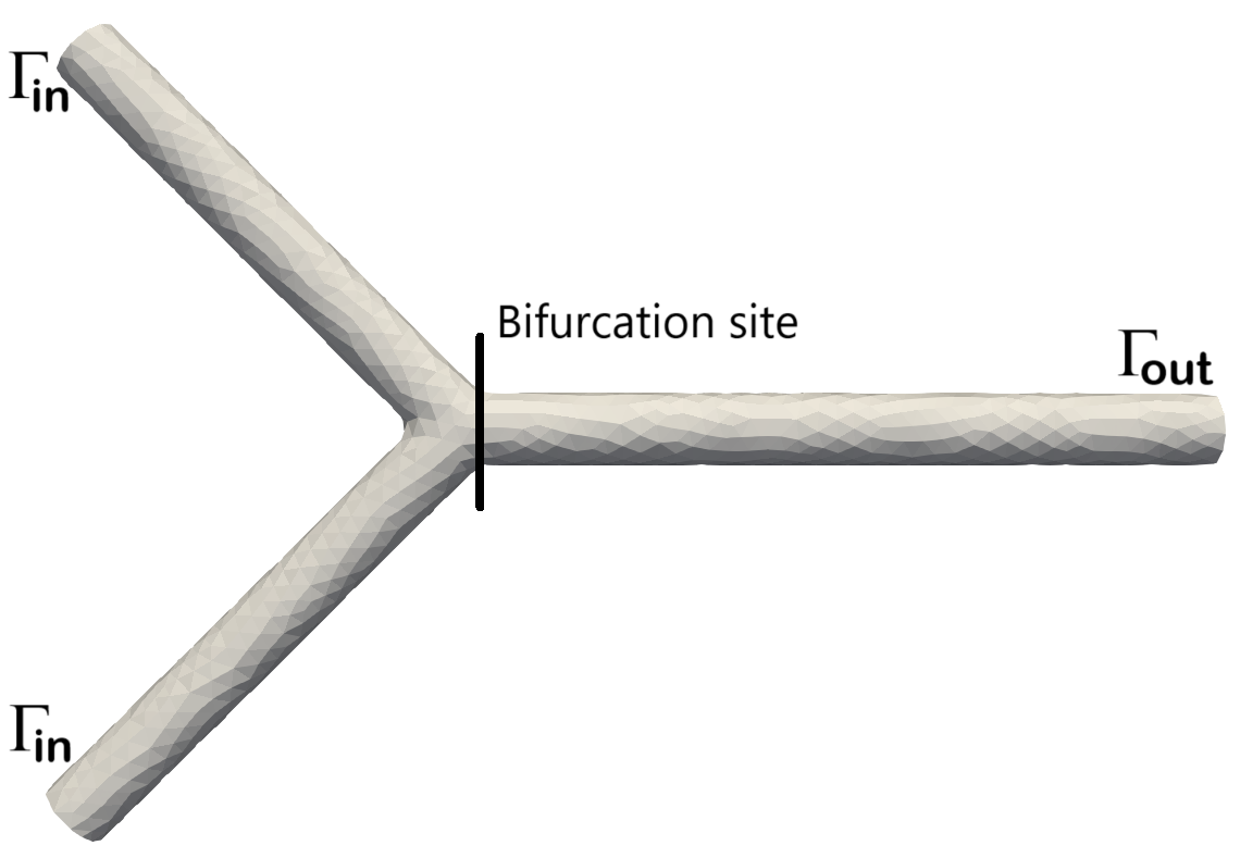
(a) Test case 1: Idealistic bifurcation model

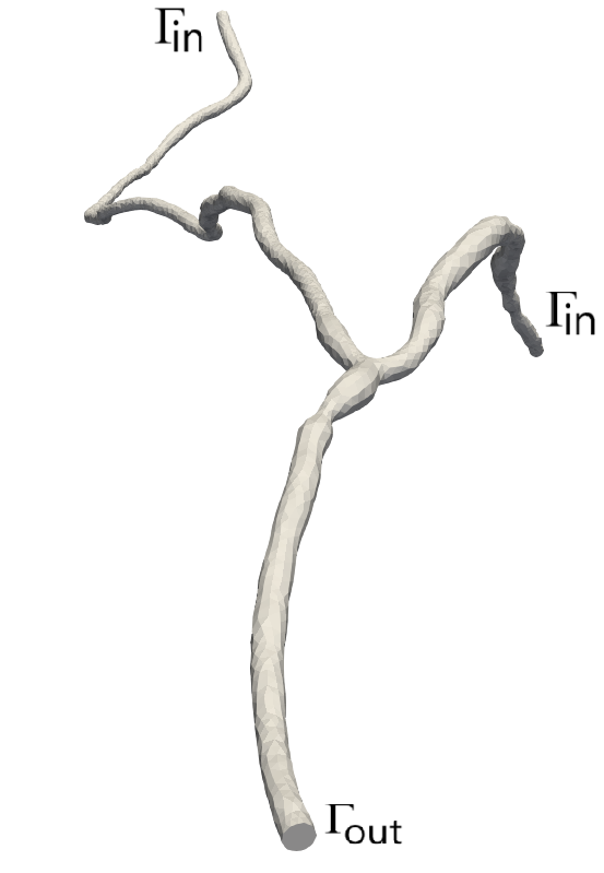
(b) Test case 2: Patient-specific CABG model

Figure 1: Three-dimensional vascular flow models.

Our objective is to minimize the discrepancy between a desired outflow velocity profile and the velocity profile achieved through the unsteady N–S equations across various parametrized inlet flow profiles. In particular, for both the idealized bifurcation and patient-specific CABG test cases, we chose the inlet flow profile defined on the inlet boundaries $\Gamma_{\mathrm{in}}$ as:

$$\bm{v}_{\mathrm{in}}=-\frac{\nu\,Re}{R_{in}}\left(1-\frac{r^{2}}{R_{in}^{2}}\right)\,f\left(t\right)\,\bm{n}_{in},$$ (51)

where $r$ represents the radius of cross-sections along the domain computed using centerlines obtained from VMTK [71], and $R_{in}$ denotes the radius of inlet cross-sections with their respective unit outward normal directions. The negative sign allows for an inflow direction, $f(t)=0.02+0.02\sin\left(\pi t\right)$ represents a time-dependent function accounting for pulsatile behaviour, and the kinematic viscosity is fixed as $\nu=3.6$ mm²/s. In blood flow problems, the non-dimensional quantity we use to parametrized the model, i.e. the Reynolds number $Re$, holds significant importance due to its influence on flow field characteristics across different regimes. For the first test case, we consider $Re$ as the parameter of the model for which we aim at reducing the computational cost. In the following, it will be denoted as $\mu=Re$, and it will vary in the parametric domain $\mathcal{D}=[50,80]$. We used a similar inlet flow profile also for the patient-specific CABG case 1(b), as real patient-specific data for the inlet conditions was not provided. For this test case, we consider the more complex setting in which each inlet flow boundary is characterized by a Reynolds number, i.e.  $\bm{\left missing}(\mu_{1},\mu_{2}\right)=\left(Re_{1},Re_{2}\right)$, where both $Re_{1}$ and $Re_{2}$ vary independently within the range $\mathcal{D}=[50,80]^{2}$. These simulations enable a thorough examination of how different inlet flow profiles, defined by varying Reynolds numbers, influence the flow behaviour and dynamics within the vascular models.

To complete the optimal control framework, the target flow velocity profile $\bm{v}_{d}$ is chosen as:

$$\bm{v}_{d}=v_{\mathrm{const}}\,\left(1-\frac{r^{2}}{R(s)^{2}}\right)\,\bm{t}\left(s\right),$$ (52)

where $\bm{t}\left(s\right)$ is the tangent along the centerline $\bm{c}\left(s\right)$, $R\left(s\right)$ is the maximum radius of the vessel around $\bm{c}\left(s\right)$, $r$ is the distance between the mesh nodes and nearest point lying on $\bm{c}\left(s\right)$, $s$ is the curvilinear abscissa, and $v_{\mathrm{const}}>0$ represents the maximum magnitude of the $\bm{v}_{d}$. As discussed in  [72], the maximum velocity of the smaller blood beds is much less than the aortic vessel and lies in the range $50-500$ mm/s, therefore, we consider $v_{\mathrm{const}}=250$ mm/s for the first test case, and we set $v_{\mathrm{const}}=100$ mm/s for the second one. For this study, we heuristically choose $\alpha=10^{-3},$ as this value provide a reasonable balance between regularization and accuracy for the computations. Table 1 contains the details of computation settings and physical parameters.

Table 1: Physical Parameters and Computational Details

Computational Parameters	Test case 1	Test case 2
Parametric Space	$Re_{1}\in[50,80]$	$\left(Re_{1},Re_{2}\right)\in[50,80]^{2}$
FE dofs	$\mathcal{N}_{h}=225^{\prime}248$	$\mathcal{N}_{h}=433^{\prime}288$
Final time	$T=1.0$ s	$T=0.8$ s
Time step	$\Delta t=0.01$ s	$\Delta t=0.01$ s
No. snapshots w.r.t. time $t$	21	21
No. snapshots w.r.t. parameter $\bm{\mu}$ $\left(=N_{\mathrm{train}}\right)$	21	25
nested-POD $\left(=N_{t}^{\mathrm{POD}}\right)$	10	10
$N_{\mathrm{max}}\left(=N_{\bm{\square}}^{\mathrm{POD}}\right)$	15	20
Offline CPU time	$\approx 4-5$ hours	$\approx 7-8$ hours
Online CPU time	$\approx 30$ minutes	$\approx 1$ hour

Performing the unsteady simulations of OCP_(μ)s for the three-dimensional model, which includes state equations, adjoint equations, and cost functionals, requires significant computational resources and memory allocation, even when $\bm{\mu}$ is fixed. Managing these simulations becomes particularly challenging due to the varying computational demands associated with different $\bm{\mu}$ values. This requires efficient allocation and utilization of computational resources to ensure that the simulations run smoothly and within acceptable time frames, despite the complexities involved. To address these computational challenges effectively, we implemented a strategy involving two intermediate steps to capture spatial-temporal information of the variables over the time interval $[0,T],$ where $T>0$ is the final time. Initially, we save information at every $k^{th}$ time-step $\left(\Delta t\right)$ out of $N_{t}$, which helped mitigate memory allocation issues during transient simulations. However, conducting simulations over the entire time interval $[0,T]$ posed challenges due to resource constraints. To address this, we adopted a sequential approach, in which initially, we saved simulation results for the time interval $[0,t_{1}]$ with $t_{1}>0$. This step allowed us to store information up to $t_{1}$ effectively managing memory usage. Subsequently, we continued the simulation from the interval $[t_{1},t_{2}]$ with $t_{2}>t_{1}$, we read the previously saved results at $t=t_{1}$, then continued the computation from $t_{1}+\Delta t$. We repeated this process until reaching the final time $T$, incrementally saving and reusing simulation data between each successive time interval. This dual-step strategy optimizes memory usage and computational efficiency, ensuring that long-duration simulations are conducted effectively without compromising on accuracy or computational performance, thus addressing the challenges posed by varying computational demands and resource limitations.

4.2 Test case 1: Idealistic Bifurcation Model

For this test case, the target flow velocity profile is computed using the steady Poiseuille flow assumption (52), a well-known analytical solution for laminar flow in a straight cylindrical pipe [73]. Figure 2 depicts the computed flow velocity profile based on the state equations, with a controlled outflow boundary and $Re=50$ at $t=0.25$ s. This high-fidelity simulation captures the intricate fluid behaviour at the bifurcation, including the effects of unsteady and viscous forces. Notably, the outlet flow velocity is higher than the inlet velocities, as mentioned in (51), a deviation from the Poiseuille flow assumption. This increase in outlet velocity arises from the convergence of flow at the bifurcation, where the merging streams must accelerate to conserve mass, as described by the continuity equation $Q_{\mathrm{inlets}}\equiv Q_{\mathrm{outlet}}.$ Figure 2 highlights the importance of detailed computational models for accurately capturing fluid dynamics in complex vascular flow geometries. In real-life scenarios, where individual anatomical features influence flow dynamics, our approach can incorporate 4D MRI data for more precise simulations. Replicating intricate behaviours, particularly near bifurcations, demonstrates the robustness of optimization problems for CV flows.

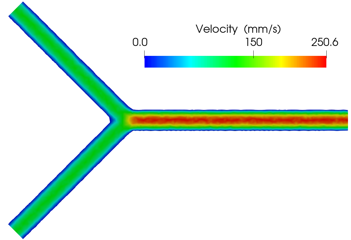
Figure 2: High-fidelity flow velocity profile with $Re=50$, and $t=0.25$ s

4.2.1 Assessment of ROM Performance

As mentioned previously in Section 4.1, we collect only $21$ snapshots in time out of the 100 time-steps solutions, for all the variables. Thus, by subsampling the time domain, we are able to ensure the accuracy utilizing a small time-step, while addressing the memory issue. In the context of nested-POD, for the temporal compression, we selected $N_{t}^{\mathrm{POD}}=10$ modes from these 21 snapshots, for each of the $N_{\mathrm{train}}=21$ parameter samples. Therefore, the resulting matrix size is $210\times\mathcal{N}_{h}$, which is significantly smaller than the matrix size $2100\times\mathcal{N}_{h}$ used in classical POD. This $90\%$ reduction not only manages memory but also accelerates computations, particularly in large-scale settings with $\mathcal{N}_{h}=225,248$, making the nested-POD approach both efficient and accurate. The offline CPU time for a fixed $\bm{\mu}$ snapshot was approximately $4-5$ hours, leading to a total offline time of around $4$ days for all $21$ snapshots. In contrast, the online CPU time was significantly reduced, taking around $30$ minutes for a snapshot, demonstrating the efficiency over the offline. Figure 3(a) shows a consistent decay of eigenvalues for state, adjoint and control variables, however, the supremizers exhibit a rapid decay. A decay of $\mathcal{O}\left(10^{-10}\right)$ in the POD singular values is achieved with fewer than $10$ POD modes, indicating a uniform representation of system dynamics during temporal compression. From Figure 3(b), we observe that pressure and supremizers show a rapid decay in normalized singular values compared to the velocity and control, they also show a significant decay, indicating that the considered system dynamics can be efficiently represented by a few modes, $N\leq 10$. Hence, Figure 3 demonstrates the efficiency of nested-POD in capturing the essential spatio-temporal features of the system with a minimal number of modes, while preserving its dynamics. The rapid decay of singular values suggests a significant reduction in computational cost without affecting accuracy.

(a) Singular values: temporal compression

(b) Singular values: parametric-space compression

Figure 3: Normalized POD singular values for velocity, pressure and supremizers.

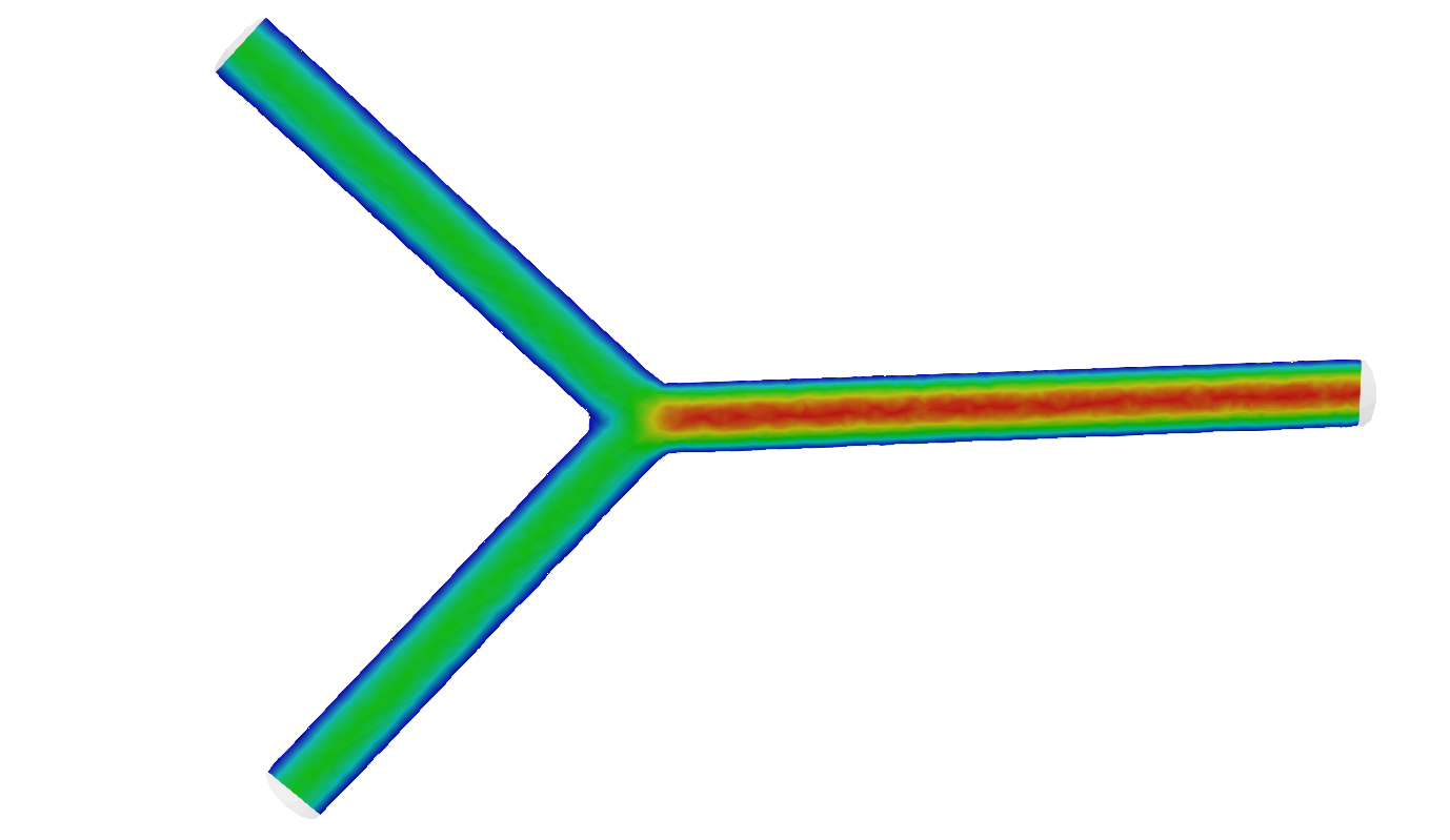
(a) High-fidelity solution

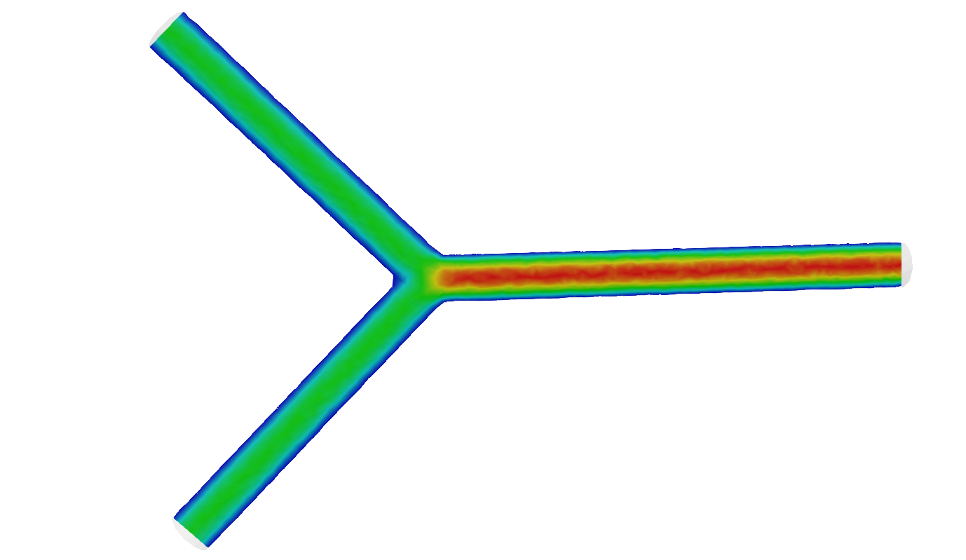
(b) Reduced-order solution

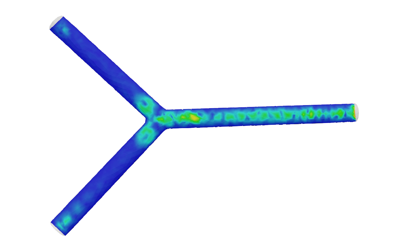
(c) Absolute error

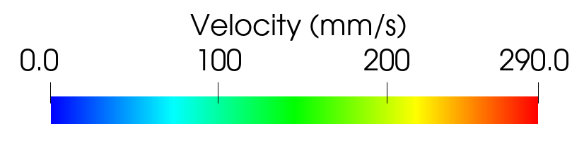
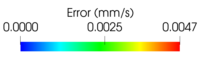
Figure 4: Comparison of velocity profiles at $Re=50$ and $t=0.5$ s. (a) High-fidelity solution, (b) Reduced-order solution, and (c) Absolute error.

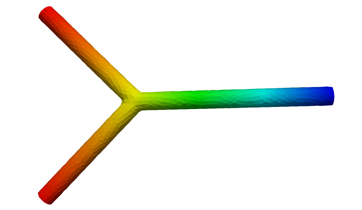
(a) High-fidelity solution

(b) Reduced-order solution

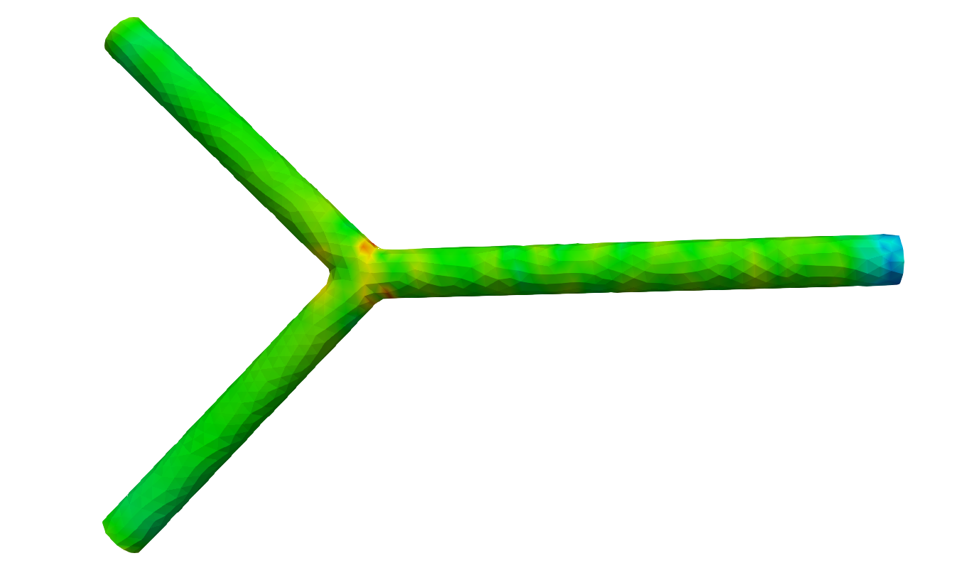
(c) Absolute error

Figure 5: Comparison of pressure distribution at $Re=50$ and $t=0.5$ s. (a) High-fidelity solution, (b) Reduced-order solution, and (c) Absolute error.

Figure 4 presents the high-fidelity and reduced order velocity profiles at maximum inlet flow profile with $Re=50$ along with the absolute error between the solutions. We have observed that the inlet flows from the inlet branches merge at the bifurcation site and exit smoothly through the outlet, as depicted in the high-fidelity solution in Figure 4(a). The fluid moves faster along the centerline, forming a parabolic velocity profile, while near the walls, the velocity gradually decreases to zero due to the rigid wall condition. The reduced order solution 4(b) closely approximates the high-fidelity solution, achieving an absolute error of order $\mathcal{O}\left(10^{-3}\right)$ with fewer POD modes. Similarly, Figure 5 shows comparable results for pressure distribution. We observe a significant pressure drop from the inlet to the outlets, where the higher inlet pressure drives the flow, and the decreasing pressure corresponds to an increase in velocity as the fluid exits. These figures demonstrate that the proposed ROM accurately reproduces the detailed velocity and pressure distributions from the Galerkin FE formulation, providing significant computational efficiency while maintaining accuracy.

4.2.2 Flow field Characteristics

Figure 6 presents the velocity distribution at the bifurcation site, illustrated in the Figure 1(a), specifically on the $xz$-plane of the domain, and the control distribution at the outflow boundary $\Gamma_{\mathrm{out}}$ at different time instances for $Re=70$. From the figure, we can investigate the flow dynamics where two inlet flows merge into a single outlet, influencing the flow characteristics such as velocity profiles and control distributions. At any fixed time $t$, we observed that the velocity profile exhibits a parabolic shape, with the highest velocity magnitude at the centre of the bifurcation site which gradually diminishes towards the walls and becomes zero due to the considered assumptions, as shown in the top row of Figure 6. As time progresses from $t=0.05$ s to $t=0.5$ s the velocity significantly increases, indicating the flow is fully developed. The velocity is influenced by the function $f\left(t\right)$, which peaks at $t=0.5$ s, subsequently, the velocity decreases.

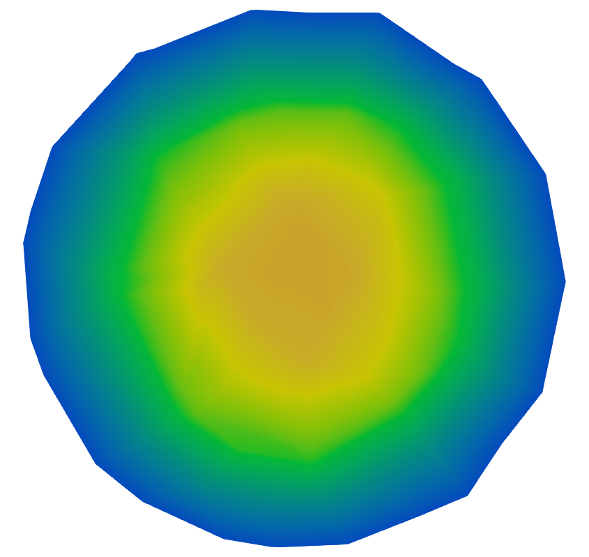
(a) $t=0.05$ s

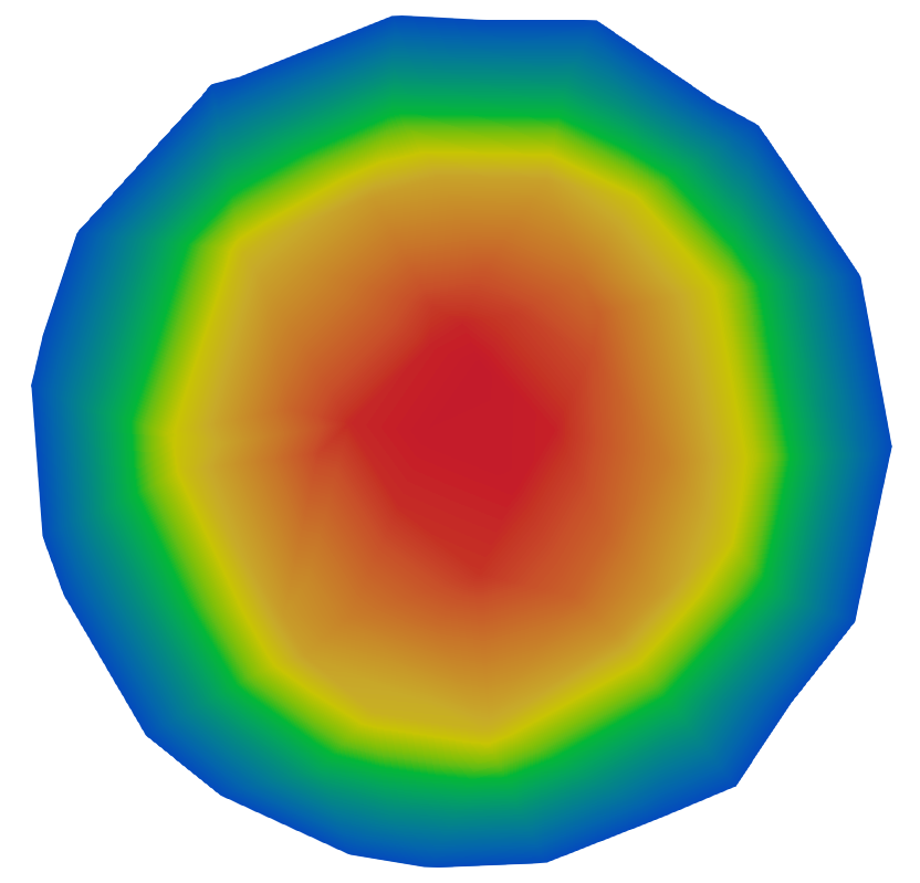
(b) $t=0.25$ s

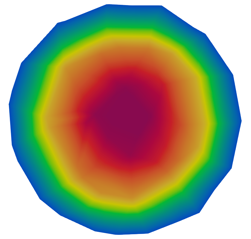
(c) $t=0.5$ s

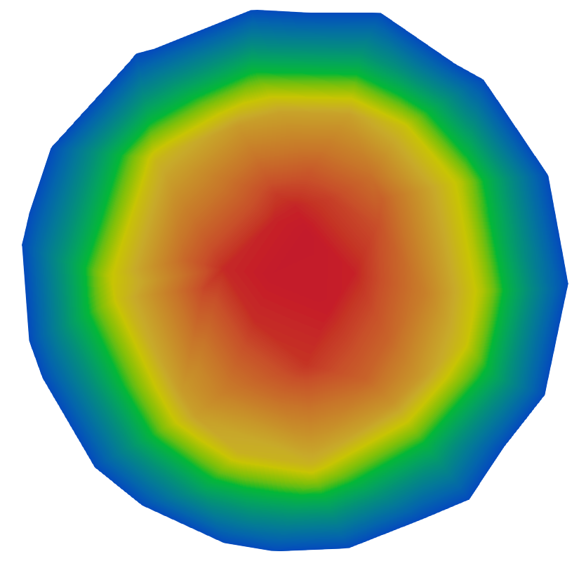
(d) $t=0.75$ s

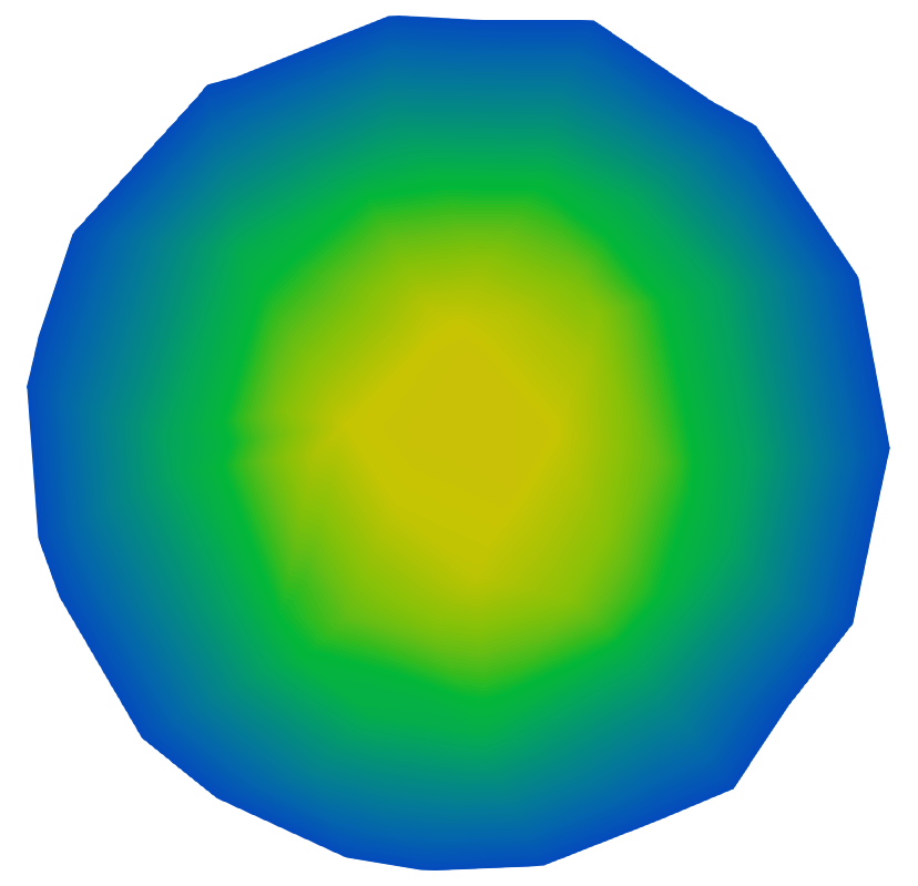
(e) $t=1.0$ s

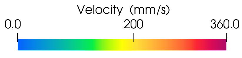
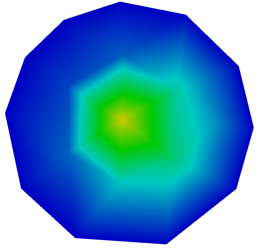
(f) $t=0.05$ s

(g) $t=0.25$ s

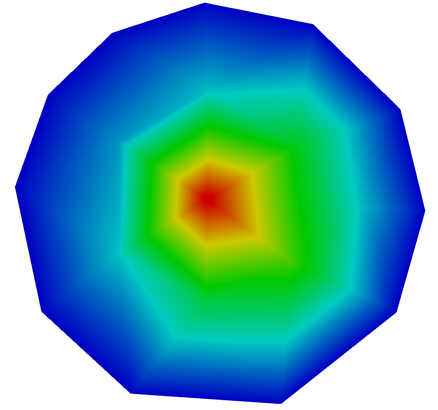
(h) $t=0.5$ s

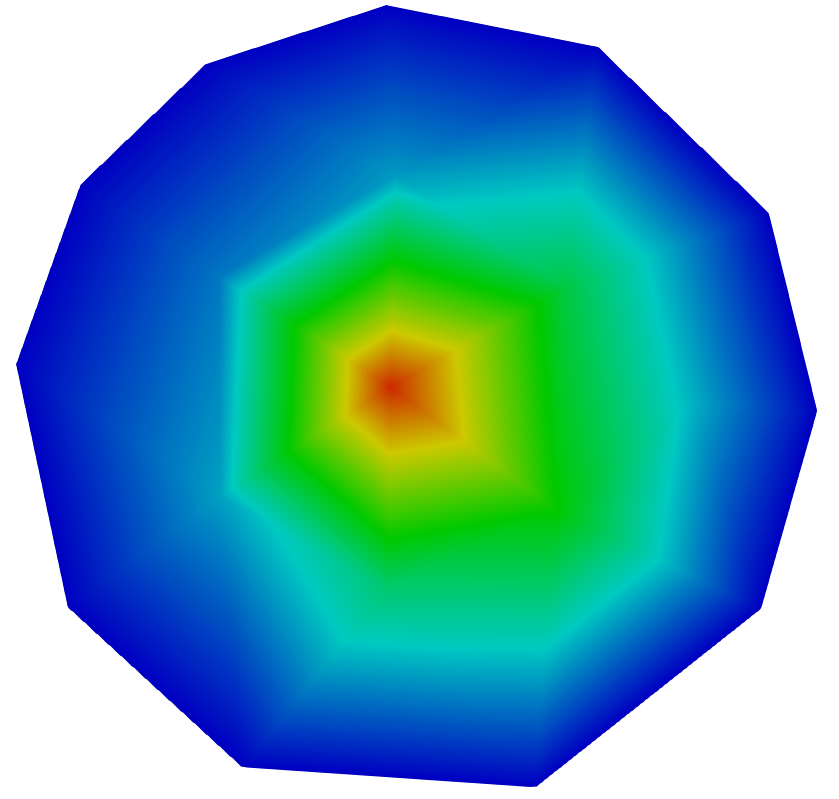
(i) $t=0.75$ s

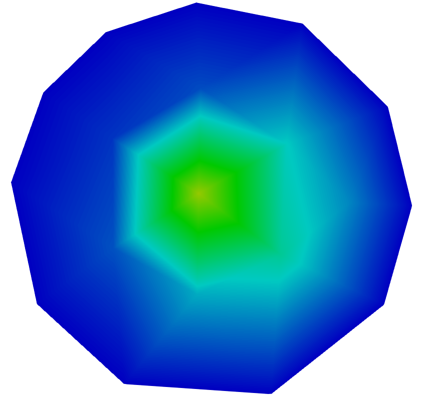
(j) $t=1.0$ s

Figure 6: Temporal variation at $Re=70$: Velocity distribution at bifurcation site (top row), and Control distribution at $\Gamma_{\mathrm{out}}$ (bottom row).

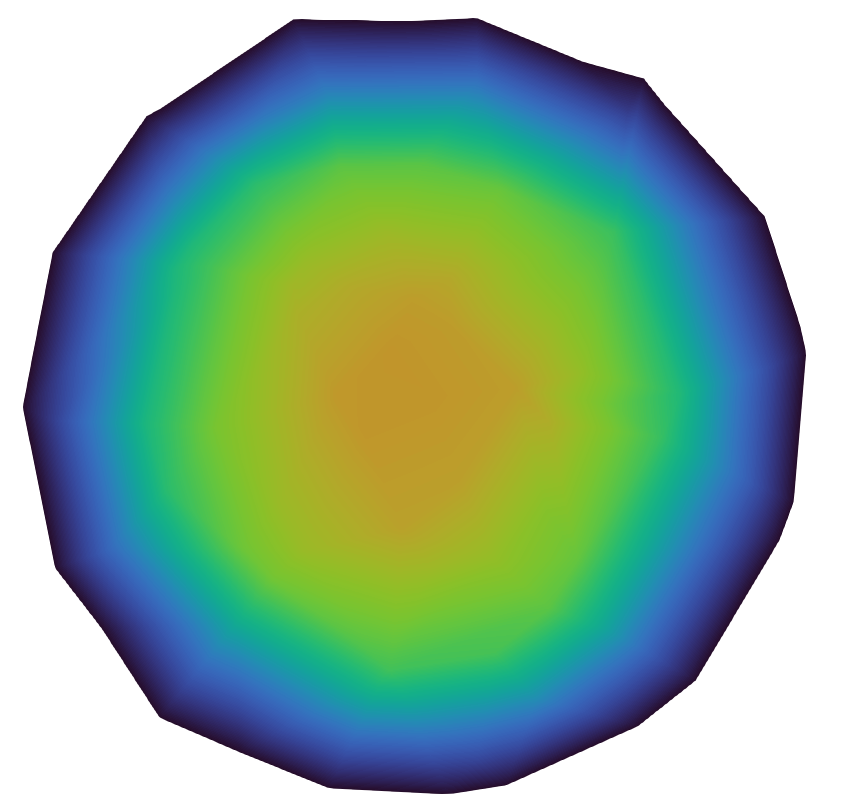
(a) $Re=50$

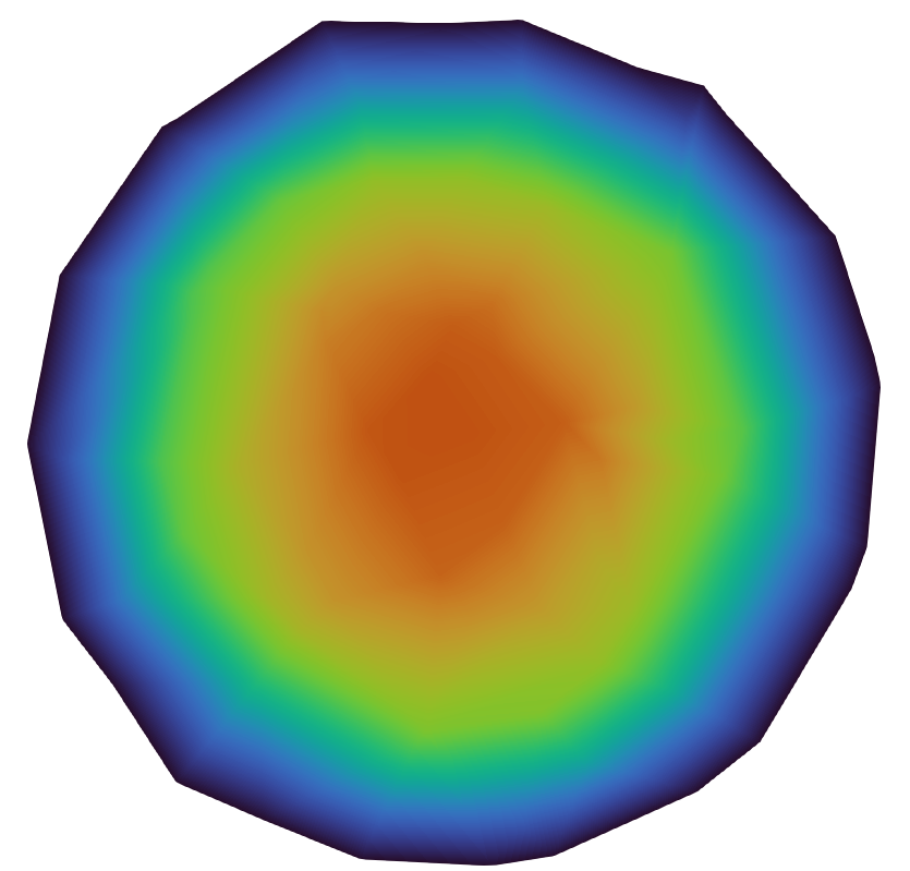
(b) $Re=60$

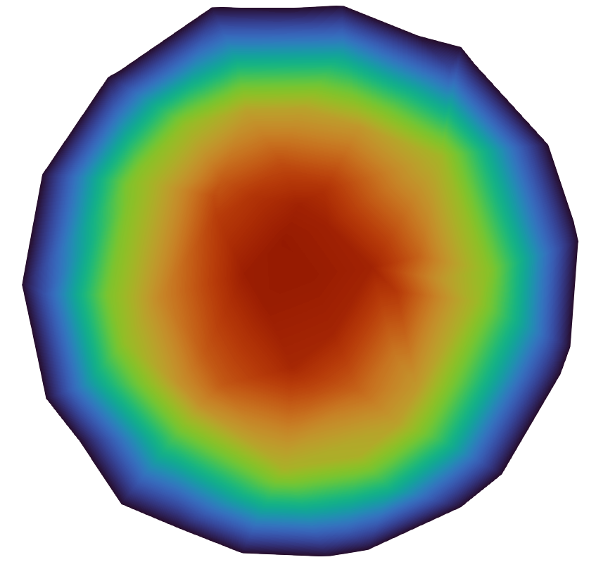
(c) $Re=70$

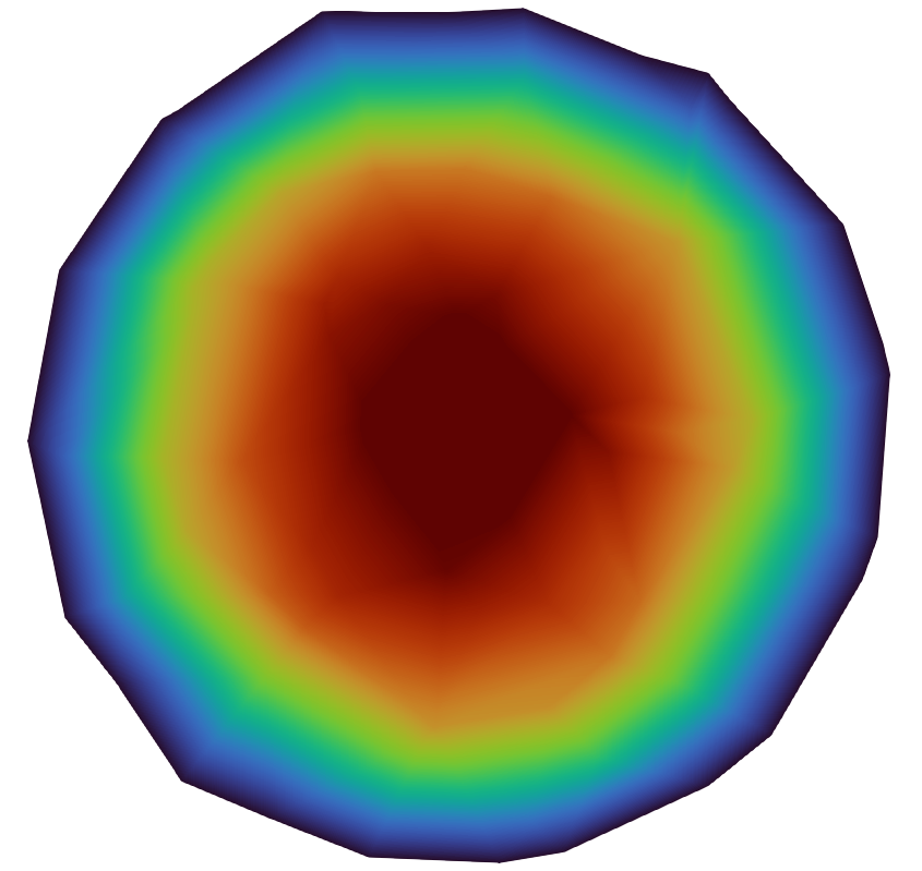
(d) $Re=80$

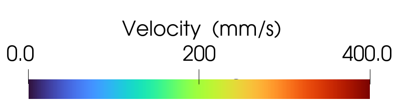
Figure 7: Parametric dependency of $Re$: Reduced-order velocity distribution at the bifurcation site at $t=0.5$ s.

The control on $\Gamma_{\mathrm{out}}$, is concentrated at the center and asymmetrically distributed with lower values toward the periphery. At time instant $t=0.05$ s, it is relatively small, effectively regulating the early flow dynamics. As time progresses, the control distribution broadens and highest around $t=0.5$ s, while still peaking at the center. After the peak, the control decreases, allowing the flow to gradually stabilize while still preserving the essential Poiseuille profile. This dynamic adjustment of control ensures smooth regulation of the flow dynamics, as depicted in the bottom row of Figure 6.

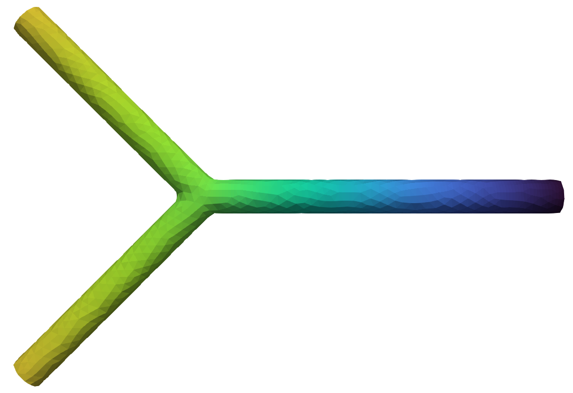
(a) $Re=50$

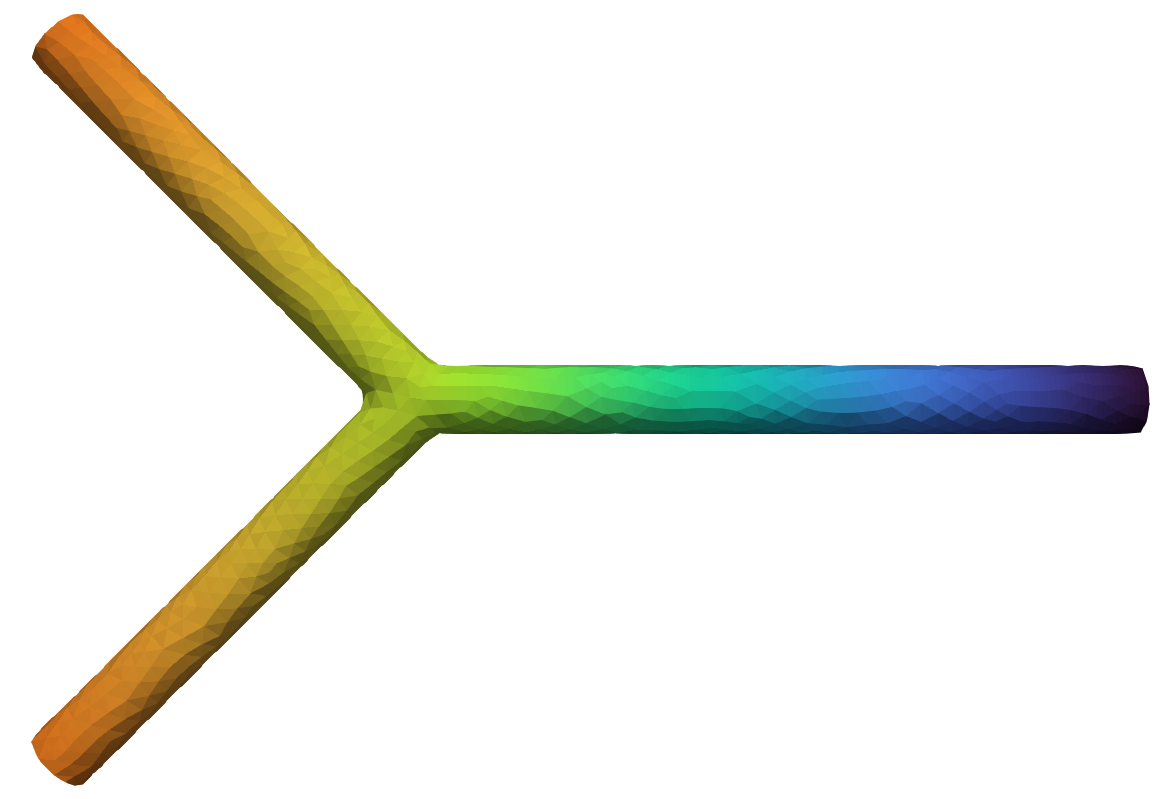
(b) $Re=60$

(c) $Re=70$

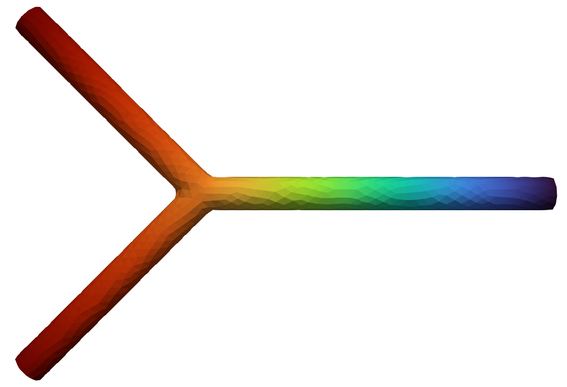
(d) $Re=80$

Figure 8: Parametric dependency of $Re$: Reduced order pressure distribution at the bifurcation site at $t=0.5$ s.

Moreover, Figures 7 and 8 present the parametric dependency of velocity and pressure distributions for various $Re$ values at $t=0.5$ s. As $Re$ increases, inertial forces dominate, leading to higher-speed flow patterns, as depicted in Figure 7. The velocity and pressure distributions are closely related; high-velocity regions correspond to low-pressure zones and vice versa, ensuring the fluid remains incompressible and momentum is balanced, as shown in Figure 8. The control at the outflow boundary significantly influences the pressure distribution, ensuring a smooth exit of merged inlet flows from the bifurcation site.

4.3 Test case 2: Patient-specific CABG

This test case, a patient-specific CABG model, represents a realistic scenario of the idealized bifurcation model presented in Test Case 4.2. The idealized bifurcation model simplifies the geometry to understand the fundamental flow dynamics, while the CABG model incorporates the complex morphology of the coronary artery, providing a more accurate and realistic simulation of CV flow dynamics. For this case, the final time is $T=0.8$ s as in [57, 31] with a time-step $\Delta t=0.01$ s, storing the solutions at every $4^{th}$ time-step, resulting in 20 snapshots in time. We considered parametric-dependent inlet flow profiles computed using Eq. (51) with $\left(Re_{1},Re_{2}\right)$ values independently within the range $[50,80]$ for each inlet boundary.

4.3.1 Assessment of ROM Performance

In this case study, we consider a patient-specific CABG model characterized by its complex morphology and a large-scale mesh comprising $\mathcal{N}_{h}=433,288$ dofs, posing significant computational challenges. Using the nested-POD approach, extracting $N_{t}^{\mathrm{POD}}=10$ POD-modes significantly reduces the dimensionality from $2500\times\mathcal{N}_{h}$ to $250\times\mathcal{N}_{h}$ with $N_{\mathrm{train}}=25$ snapshots, for capturing the dominant dynamics of the system. Each $\bm{\mu}$ snapshot in the offline phase required about $7-8$ hours, adding up to approximately $8$ days for all snapshots. In contrast, the online phase significantly enhanced efficiency, reducing the CPU time to around $1$ hour per snapshot, resulting in substantial time savings. Figure 9 presents POD singular values and retained energy for all variables during the temporal and parametric-space compression. We observed that state velocity, adjoint velocity, and control exhibit significant decay in normalized singular values, while pressure and supremizers show a more rapid decay. This suggests the system dynamics can be captured with a reduced number of POD modes $N\leq 20$. Additionally, we noticed that state variables decay more slowly compared to adjoint variables, and retaining the $95\%$ energy of the system, as shown in Figures 9(c) and 9(d). Subsequently, the essential spatio-temporal features of the cardiovascular system are accurately captured using a minimal number of POD modes, highlighting the effectiveness of the proposed approach.

(a) Singular values: temporal compression

(b) Singular values: parametric-space compression

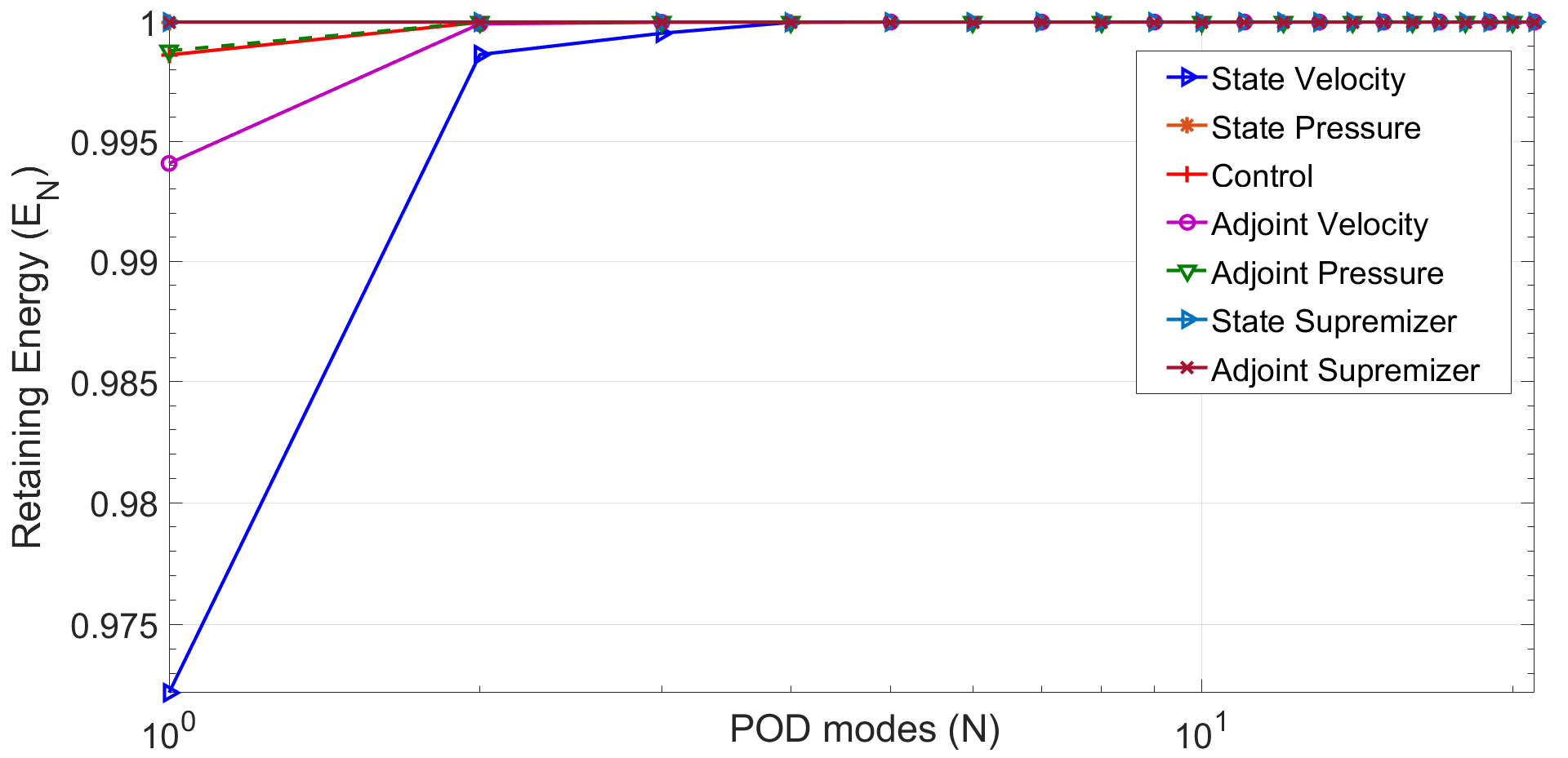
(c) Retaining energy: temporal compression

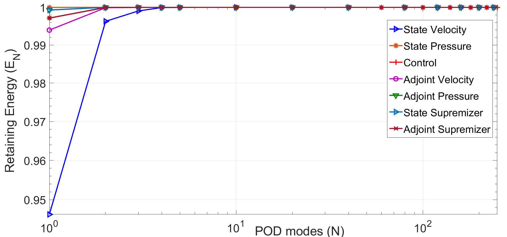
(d) Retaining energy: parametric-space compression

Figure 9: Normalized POD singular values (top row) and retaining energy (bottom row) for velocity, pressure, and supremizers.

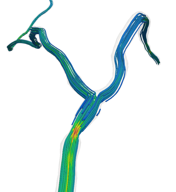
(a) High-fidelity solution

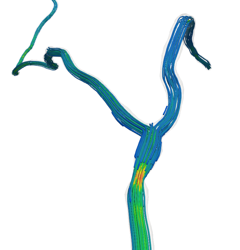
(b) Reduced-order solution

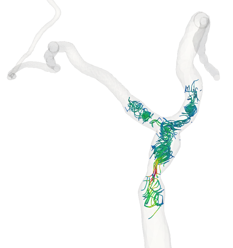
(c) Absolute error

Figure 10: Comparison of the streamlines at $\left(Re_{1},Re_{2}\right)=\left(80,80\right)$ and $t=0.4$ s. (a) High-fidelity solution, (b) Reduced-order solution, and (c) Absolute error.

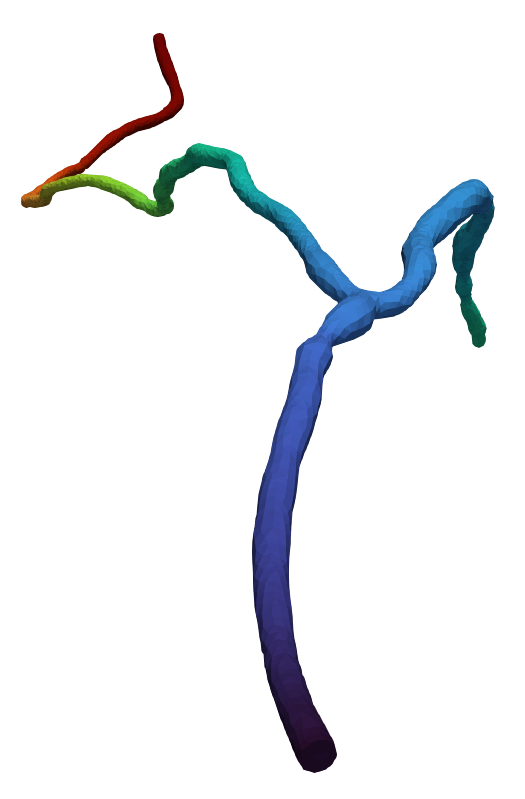
(a) High-fidelity solution

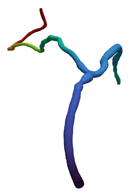
(b) Reduced-order solution

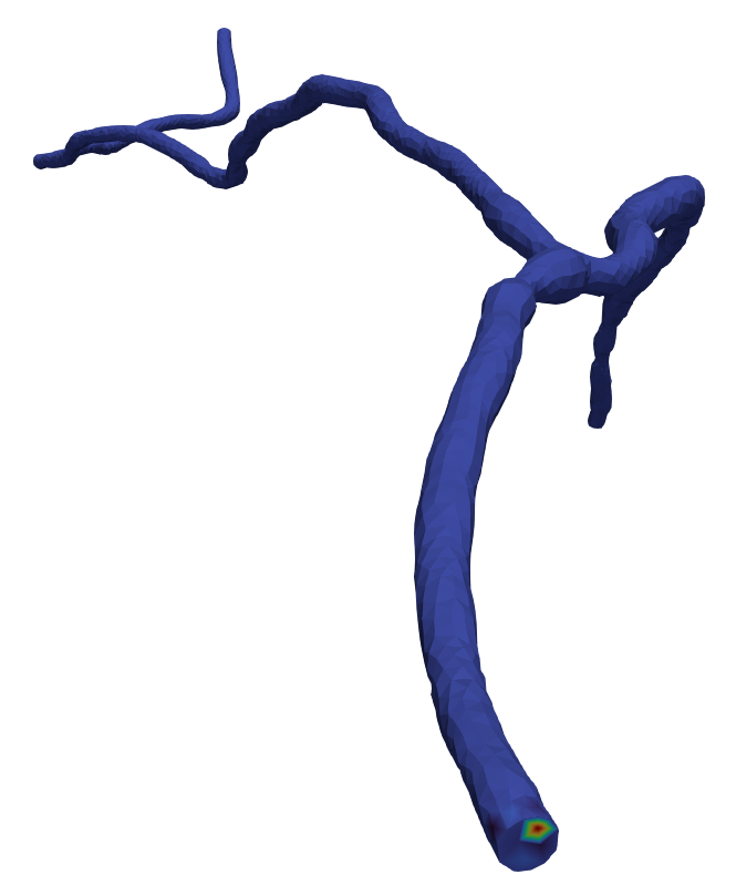
(c) Absolute error

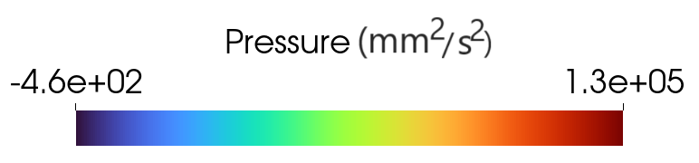
Figure 11: Comparison of pressure distributions at $\left(Re_{1},Re_{2}\right)=\left(80,80\right)$ and $t=0.4$ s. (a) High-fidelity solution, (b) Reduced-order solution, and (c) Absolute error.

Figures 10 and 11 illustrate the comparison between the high-fidelity solutions and reduced-order model approximations for both streamlines and pressure variations, along with the corresponding absolute errors between the two methods at $\left(Re_{1},Re_{2}\right)=\left(80,80\right)$ and $t=0.4$ s. The streamlines in Figure 10(a) show the flow behavior in a patient-specific CABG model, where fluid enters through the RIMA and LAD inlets and exits through the outlet, with high velocities observed in the outlet and region of stenoses. The high-fidelity solutions capture the intricate flow dynamics and detail pressure variations, while the reduced-order models offer computationally efficient approximations. The error plots reveal where the reduced-order models deviate from the high-fidelity solutions, particularly in areas with complex flow behaviors, such as regions with stenosis, and sharp pressure gradients. These comparisons demonstrate the effectiveness of reduced-order models in accurately approximating the high-fidelity solutions while significantly reducing computational costs, making them a valuable tool for efficient and reliable simulations in patient-specific modelling.

4.3.2 Flow field Characteristics

Figure 12 depicts the control distribution at the outflow boundary $\Gamma_{\mathrm{out}}$ and wall shear stress (WSS) distributions at different time instances with $\left(Re_{1},Re_{2}\right)=\left(80,50\right)$. WSS is a crucial parameter in CV flows because it directly influences endothelial cell functions [74, 75, 24]. It is defined as the tangential force exerted by blood flow on the endothelial surface of the vessels, expressed by:

$$\bm{\tau}_{w}=\nu\,\Big{(}\nabla\left(\bm{v}\right)+\nabla\left(\bm{v}\right)^{\top}\Big{)}\cdot\bm{n}.$$ (53)

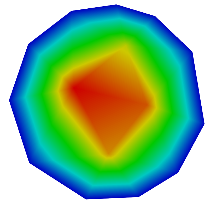
(a) $t=0.04$ s

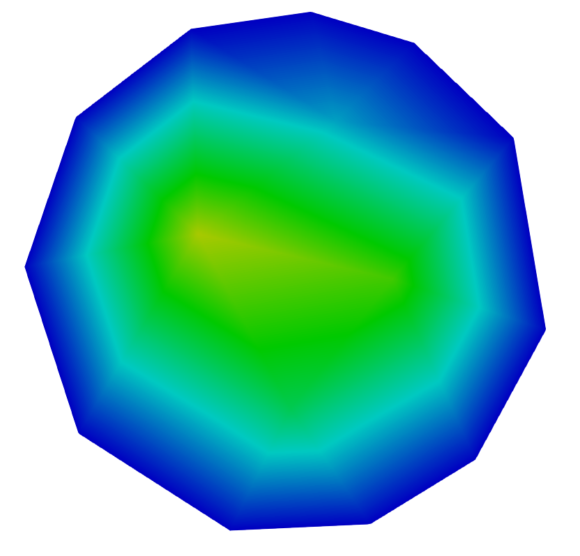
(b) $t=0.2$ s

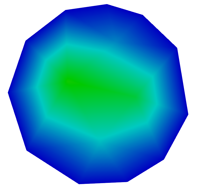
(c) $t=0.4$ s

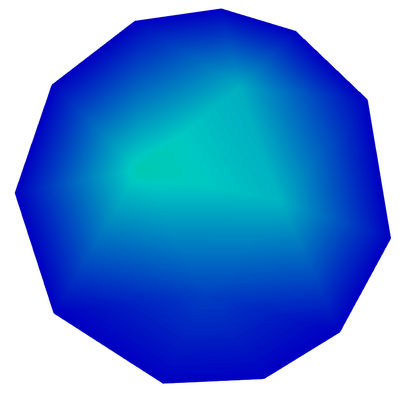
(d) $t=0.6$ s

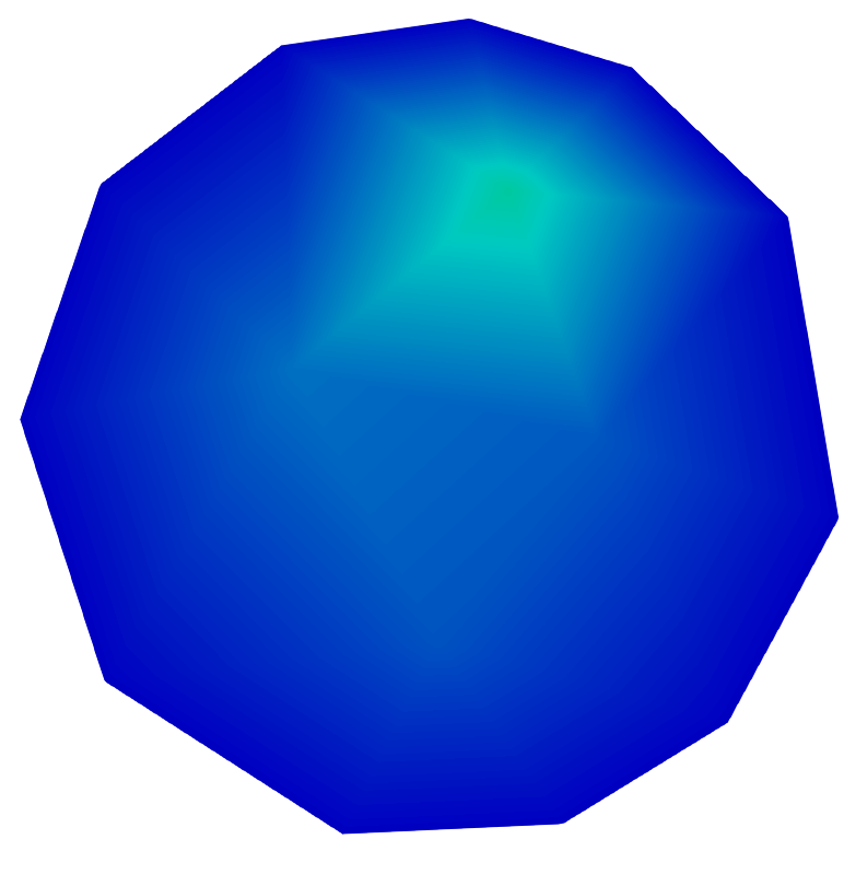
(e) $t=0.8$ s

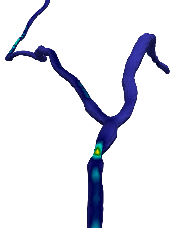
(f) $t=0.04$ s

(g) $t=0.2$ s

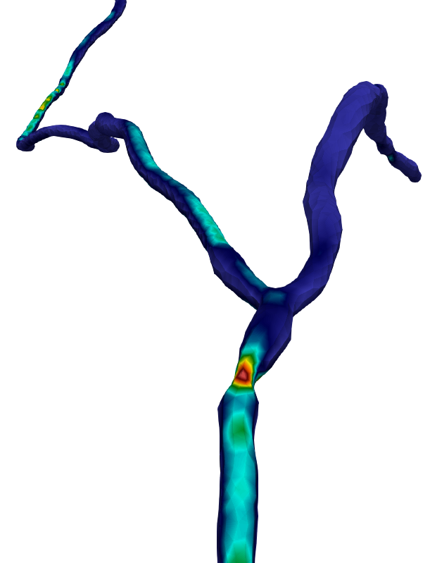
(h) $t=0.4$ s

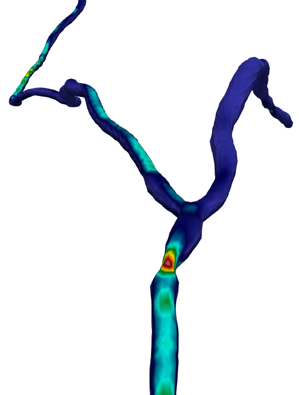
(i) $t=0.6$ s

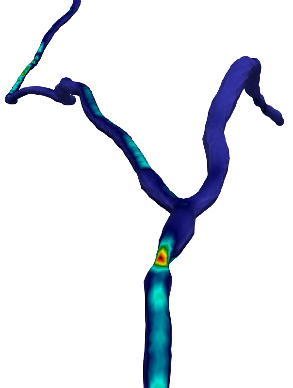
(j) $t=0.8$ s

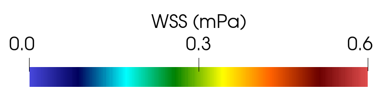
Figure 12: Temporal variation with $\left(Re_{1},Re_{2}\right)=\left(80,50\right)$: Control distributions at $\Gamma_{\mathrm{out}}$ (top row) and WSS distribution (bottom row).

From Figure 12, the flow dynamics are observed as two inlet flows merge into a single outlet, significantly affecting both the flow characteristics and control distributions. At time instance $t=0.04$ s, the control is strongly distributed across the center of $\Gamma_{\mathrm{out}}$, exerting a significant influence to regulate the early, developing flow dynamics. Correspondingly, the WSS is relatively low throughout most of the vessel, but concentrated in regions of stenosis, where the flow merges and accelerates, leading to higher stress on the vessel walls. As time progresses, particularly by $t=0.2$ s and $t=0.4$ s, the control weakens, spreading with lower values toward the outer regions. However, the WSS increases during this time, especially in areas with high flow velocities such as near the bifurcation and stenosis. This suggests that, even though the control is becoming less dominant, the flow itself is maturing and generating stronger interactions with the vessel walls, leading to higher WSS. By $t=0.8$ s, the control becomes significantly smaller, indicating that the flow is fully developed and no longer requires stress to regulate; however, WSS remains concentrated within the same critical regions. WSS is directly proportional to the velocity gradients at the wall; a steeper gradient leads to higher WSS due to the greater difference in velocity between the fluid near the wall and that further away. The region of high WSS corresponds to the high-velocity regions as depicted in Figure 10(a). The observed temporal variations in control and WSS are due to the inter-dependency between the state, adjoint, and control solutions. This interdependency can be understood from the Eqs. (5), (16) and (17), which ensure that the control effectively regulates the state velocity with the objective and optimality conditions.

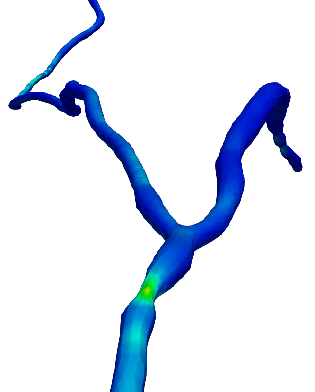
(a) $\left(Re_{1},Re_{2}\right)=\left(50,50\right)$

(b) $\left(Re_{1},Re_{2}\right)=\left(50,70\right)$

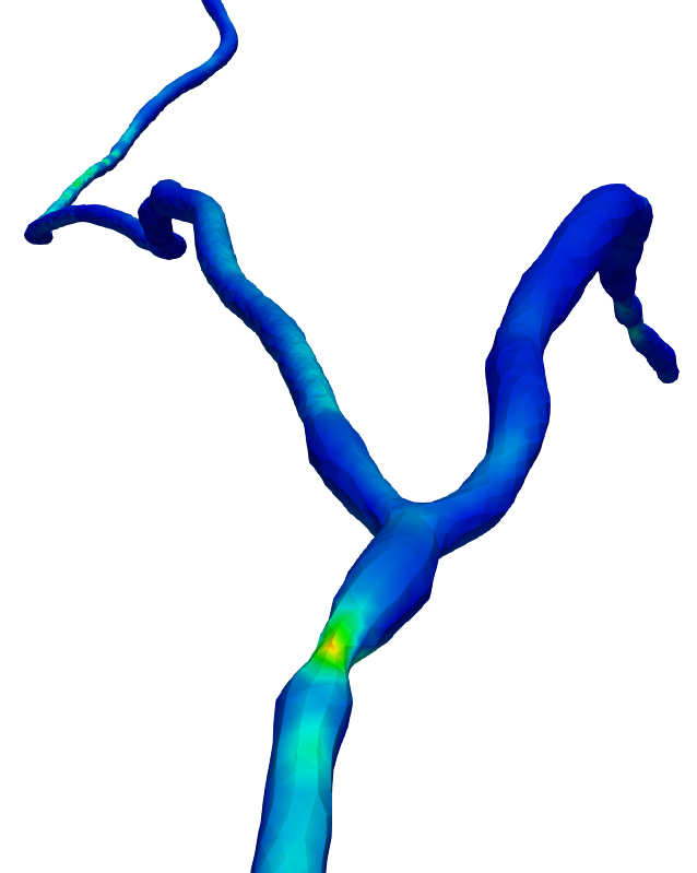
(c) $\left(Re_{1},Re_{2}\right)=\left(60,60\right)$

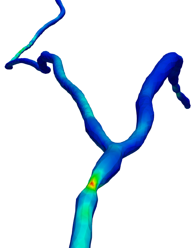
(d) $\left(Re_{1},Re_{2}\right)=\left(70,70\right)$

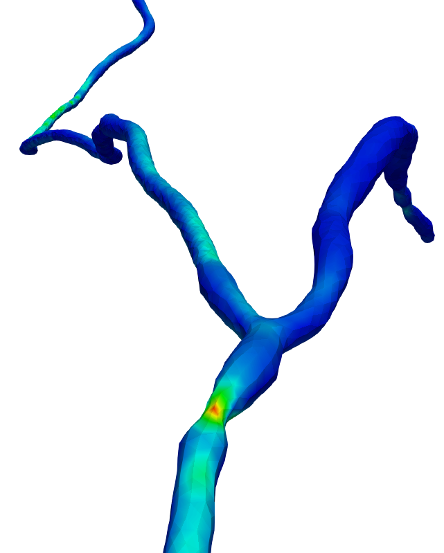
(e) $\left(Re_{1},Re_{2}\right)=\left(80,50\right)$

(f) $\left(Re_{1},Re_{2}\right)=\left(80,80\right)$

Figure 13: Parametric dependency of $\left(Re_{1},Re_{2}\right)$ values on reduced order WSS distributions at $t=0.4$ s.

In Figure 13, the WSS distribution shows how the shear stress is affected by different combinations of Reynolds numbers. When the $Re$ value is same at both inlets $\Gamma_{\mathrm{in}},$ as shown in Figures 13(a), 13(c) 13(d) and 13(f), WSS distribution is symmetric, and as $Re$ increases, the WSS also increases, especially in critical regions such as bifurcations and stenosis. This is because higher $Re$ values lead to higher flow velocity, which increases the shear stress on the vessel walls. However, a notable difference is observed when comparing the WSS values from Figures 13(b) and 13(e) and Figures 13(d) and 13(e), respectively. In Figure 13(b), we have $\left(Re_{1},Re_{2}\right)=\left(50,70\right)$, and the WSS distribution is asymmetric due to the difference in $Re$ between the two inlets. The inlet with $Re=70$ experiences higher WSS than the inlet with $Re=50$. A similar pattern occurs for the Figure 13(e); even though, it has a higher $Re$ of $80$ in one inlet, the overall WSS is lower than in Figure 13(d), where both inlets have an same $Re$ values of $70.$ This occurs because the inlet flow with $Re=50$ in Figure 13(e) has a slower flow rate, which lowers the overall WSS. Such different flow conditions, where one inlet has a much lower $Re$, reduce the overall shear stress, despite the other inlet experiencing high stress due to a high Reynolds number.

5 Conclusion

This study successfully introduced a projection-based reduced approach for solving parameterized optimization problems related with the unsteady N-S equations, with a specific focus on computing CV flows. The technique was applied to efficiently control outflow conditions, essential for regulating flow dynamics in both an idealistic bifurcation geometry and a patient-specific CABG model. Figure 2 shows minimal discrepancies between the target and computed velocity profiles, demonstrating that we have achieved our objective and highlighting the robustness of our optimization-based framework for CV flows. These simulations, especially for complex geometries and patient-specific data, can be computationally expensive. We observed that our proposed ROM effectively captures the essential dynamics of the flow fields while substantially reducing computational costs compared to high-fidelity solutions. The speed-up achieved by the ROM, which is approximately 8 times faster than a high-fidelity solution as shown in Table 1 for both the test cases, underscores its advantage in accelerating simulations over traditional high-fidelity computations. Figures 4,  5,  10 and  11, demonstrate that this reduced methodology effectively reproduces the detailed features observed in the Galerkin FE formulation for both velocity and pressure distributions in vascular models at the specified Reynolds number and time. The configured outflow boundary condition ensures that the control strategy can dynamically adjust to optimize blood flow essential for maintaining stable and efficient flow within the computational domain, as shown in Figures 6 and 12. These analysis further confirms that WSS and control distributions, maintaining consistency with the desired flow dynamics, while the outlet pressure decreases from Figure 8. Given the critical role of the outflow boundary in CV flows [22, 24], our control strategy is crucial for capturing detailed flow dynamics and ensuring effective flow regulation. These findings highlight the importance of precise control in maintaining efficient hemodynamics and realistic physiological behaviour. Figure 13 show that WSS depends on whether the $Re$ values are the same or different between the inlets, with equal $Re$ leading to higher and more consistent WSS, while different $Re$ values can lower WSS in one inlet despite high stress in the other. In clinical practice, high WSS is associated with increased risks of vascular damage, atherosclerosis, or remodelling, particularly in bifurcation and stenotic regions with high Reynolds number flows [74, 75]. This ROM approach demonstrates a robust and efficient methodology for simulating complex CV flows, providing significant computational savings without compromising accuracy. Its application to both idealized and patient-specific models underscores its potential for real-time simulations and large-scale cardiovascular studies, making it a valuable tool for advancing patient-specific modelling and improving clinical outcomes.

Conflict of Interest

We hereby declare that all the authors have no potential conflict of interest.

Author contributions

SR: Conceptualization, Methodology, Software, Formal Analysis, Investigation, Visualization, Writing-Original Draft, Review & Editing; PCA: Conceptualization, Methodology, Formal Analysis, Writing-Review & Editing, Supervision; FB: Conceptualization, Methodology, Software, Formal Analysis, Writing-Review & Editing; FP: Conceptualization, Methodology, Formal Analysis, Writing-Review & Editing; MG: Formal Analysis, Writing-Review & Editing; GR: Funding Acquisition, Project Administration, Writing-Review.

References

- [1] Max Gunzburger. Adjoint equation-based methods for control problems in incompressible, viscous flows. Flow, Turbulence and Combustion, 65:249–272, 2000.
- [2] Max D Gunzburger. Perspectives in flow control and optimization. SIAM, 2002.
- [3] Pavel Bochev and Max D Gunzburger. Least-squares finite-element methods for optimization and control problems for the stokes equations. Computers & Mathematics with Applications, 48(7-8):1035–1057, 2004.
- [4] Michael Hinze, René Pinnau, Michael Ulbrich, and Stefan Ulbrich. Optimization with PDE constraints, volume 23. Springer Science & Business Media, 2008.
- [5] Pavel B Bochev and Max D Gunzburger. Least-squares finite element methods, volume 166. Springer Science & Business Media, 2009.
- [6] Alfio Quarteroni, Gianluigi Rozza, Luca Dedè, and Annalisa Quaini. Numerical approximation of a control problem for advection-diffusion processes. In System Modeling and Optimization: Proceedings of the 22nd IFIP TC7 Conference held from July 18–22, 2005, in Turin, Italy 22, pages 22–29. Springer, 2006.
- [7] Matthias Gerdts. Global convergence of a nonsmooth newton method for control-state constrained optimal control problems. SIAM Journal on Optimization, 19(1):326–350, 2008.
- [8] Jacques Louis Lions. Optimal control of systems governed by partial differential equations, volume 170. Springer, 1971.
- [9] Jacques Louis Lions. Some aspects of the optimal control of distributed parameter systems. SIAM, 1972.
- [10] Qun Lin, Ryan Loxton, and Kok Lay Teo. The control parameterization method for nonlinear optimal control: a survey. Journal of Industrial and management optimization, 10(1):275–309, 2014.
- [11] Gamal N Elnagar. State-control spectral chebyshev parameterization for linearly constrained quadratic optimal control problems. Journal of Computational and Applied Mathematics, 79(1):19–40, 1997.
- [12] Kok Lay Teo, Bin Li, Changjun Yu, Volker Rehbock, et al. Applied and computational optimal control. Optimization and Its Applications, 2021.
- [13] Andrea Manzoni and Federico Negri. Heuristic strategies for the approximation of stability factors in quadratically nonlinear parametrized pdes. Advances in Computational Mathematics, 41:1255–1288, 2015.
- [14] Fabio Nobile and Tommaso Vanzan. A combination technique for optimal control problems constrained by random pdes. SIAM/ASA Journal on Uncertainty Quantification, 12(2):693–721, 2024.
- [15] Chamakuri Nagaiah and Karl Kunisch. Higher order optimization and adaptive numerical solution for optimal control of monodomain equations in cardiac electrophysiology. Applied numerical mathematics, 61(1):53–65, 2011.
- [16] Nakeya D Williams, Jesper Mehlsen, Hien T Tran, and Mette S Olufsen. An optimal control approach for blood pressure regulation during head-up tilt. Biological cybernetics, 113(1):149–159, 2019.
- [17] Adel M Malek, Seth L Alper, and Seigo Izumo. Hemodynamic shear stress and its role in atherosclerosis. Jama, 282(21):2035–2042, 1999.
- [18] Francis Loth, Paul F Fischer, and Hisham S Bassiouny. Blood flow in end-to-side anastomoses. Annu. Rev. Fluid Mech., 40:367–393, 2008.
- [19] Brenda R Kwak, Magnus Bäck, Marie-Luce Bochaton-Piallat, Giuseppina Caligiuri, Mat JAP Daemen, Peter F Davies, Imo E Hoefer, Paul Holvoet, Hanjoong Jo, Rob Krams, et al. Biomechanical factors in atherosclerosis: mechanisms and clinical implications. European heart journal, 35(43):3013–3020, 2014.
- [20] Danny Bluestein. Utilizing computational fluid dynamics in cardiovascular engineering and medicine—what you need to know. its translation to the clinic/bedside. Artificial organs, 41(2):117, 2017.
- [21] Alfio Quarteroni, Massimiliano Tuveri, and Alessandro Veneziani. Computational vascular fluid dynamics: problems, models and methods. Computing and Visualization in Science, 2:163–197, 2000.
- [22] Irene E Vignon-Clementel, CA Figueroa, KE Jansen, and CA Taylor. Outflow boundary conditions for 3d simulations of non-periodic blood flow and pressure fields in deformable arteries. Computer methods in biomechanics and biomedical engineering, 13(5):625–640, 2010.
- [23] Mahdi Esmaily Moghadam, Yuri Bazilevs, Tain-Yen Hsia, Irene E Vignon-Clementel, Alison L Marsden, and Modeling of Congenital Hearts Alliance (MOCHA). A comparison of outlet boundary treatments for prevention of backflow divergence with relevance to blood flow simulations. Computational Mechanics, 48:277–291, 2011.
- [24] Surabhi Rathore, Tomoki Uda, Viet QH Huynh, Hiroshi Suito, Toshitaka Watanabe, Hironobu Sugiyama, and D Srikanth. Numerical computation of blood flow for a patient-specific hemodialysis shunt model. Japan Journal of Industrial and Applied Mathematics, 38(3):903–919, 2021.
- [25] Surabhi Rathore, Hironobu Sugiyama, and Hiroshi Suito. Computational analysis for competition flows in arteriovenous fistulas based on non-contrast magnetic resonance imaging. arXiv preprint arXiv:2308.15217, 2023.
- [26] Pasquale Claudio Africa, Ivan Fumagalli, Michele Bucelli, Alberto Zingaro, Marco Fedele, Alfio Quarteroni, et al. lifex-cfd: An open-source computational fluid dynamics solver for cardiovascular applications. Computer Physics Communications, 296:109039, 2024.
- [27] Alan S Go, Dariush Mozaffarian, Véronique L Roger, Emelia J Benjamin, Jarett D Berry, Michael J Blaha, Shifan Dai, Earl S Ford, Caroline S Fox, Sheila Franco, et al. Heart disease and stroke statistics—2014 update: a report from the american heart association. circulation, 129(3):e28–e292, 2014.
- [28] Sethuraman Sankaran, Mahdi Esmaily Moghadam, Andrew M Kahn, Elaine E Tseng, Julius M Guccione, and Alison L Marsden. Patient-specific multiscale modeling of blood flow for coronary artery bypass graft surgery. Annals of biomedical engineering, 40:2228–2242, 2012.
- [29] Valery Agoshkov, Alfio Quarteroni, and Gianluigi Rozza. Shape design in aorto-coronaric bypass anastomoses using perturbation theory. SIAM Journal on Numerical Analysis, 44(1):367–384, 2006.
- [30] Rosalyn Scott, Eugene H Blackstone, Patrick M McCarthy, Bruce W Lytle, Floyd D Loop, Jennifer A White, and Delos M Cosgrove. Isolated bypass grafting of the left internal thoracic artery to the left anterior descending coronary artery: late consequences of incomplete revascularization. The Journal of thoracic and cardiovascular surgery, 120(1):173–184, 2000.
- [31] Francesco Ballarin, Elena Faggiano, Andrea Manzoni, Alfio Quarteroni, Gianluigi Rozza, Sonia Ippolito, Carlo Antona, and Roberto Scrofani. Numerical modeling of hemodynamics scenarios of patient-specific coronary artery bypass grafts. Biomechanics and modeling in mechanobiology, 16:1373–1399, 2017.
- [32] Joshua Michael Rosenblum, Jose Binongo, Jane Wei, Yuan Liu, Bradley G Leshnower, Edward P Chen, Jeffrey S Miller, Steven K Macheers, Omar M Lattouf, Robert A Guyton, et al. Priorities in coronary artery bypass grafting: is midterm survival more dependent on completeness of revascularization or multiple arterial grafts? The journal of thoracic and cardiovascular surgery, 161(6):2070–2078, 2021.
- [33] Pierfrancesco Siena, Michele Girfoglio, Francesco Ballarin, and Gianluigi Rozza. Data-driven reduced order modelling for patient-specific hemodynamics of coronary artery bypass grafts with physical and geometrical parameters. Journal of Scientific Computing, 94(2):38, 2023.
- [34] Gianluigi Rozza. On optimization, control and shape design of an arterial bypass. International Journal for Numerical Methods in Fluids, 47(10-11):1411–1419, 2005.
- [35] Elisa Fevola, Francesco Ballarin, Laura Jiménez-Juan, Stephen Fremes, Stefano Grivet-Talocia, Gianluigi Rozza, and Piero Triverio. An optimal control approach to determine resistance-type boundary conditions from in-vivo data for cardiovascular simulations. International Journal for Numerical Methods in Biomedical Engineering, 37(10):e3516, 2021.
- [36] Gianluigi Rozza, Andrea Manzoni, and Federico Negri. Reduction strategies for pde-constrained optimization problems in haemodynamics. In Proceedings of the 6th European Congress on Computational Methods in Applied Sciences and Engineering, pages 1748–1769. Vienna Technical University, 2012.
- [37] Alfio Quarteroni, Gianluigi Rozza, et al. Reduced order methods for modeling and computational reduction, volume 9. Springer, 2014.
- [38] Toni Lassila, Andrea Manzoni, Alfio Quarteroni, and Gianluigi Rozza. Model order reduction in fluid dynamics: challenges and perspectives. Reduced Order Methods for modeling and computational reduction, pages 235–273, 2014.
- [39] Maria Strazzullo, Francesco Ballarin, and Gianluigi Rozza. Pod-galerkin model order reduction for parametrized nonlinear time-dependent optimal flow control: an application to shallow water equations. Journal of Numerical Mathematics, 30(1):63–84, 2022.
- [40] Federico Pichi, Maria Strazzullo, Francesco Ballarin, and Gianluigi Rozza. Driving bifurcating parametrized nonlinear pdes by optimal control strategies: application to navier–stokes equations with model order reduction. ESAIM: Mathematical Modelling and Numerical Analysis, 56(4):1361–1400, 2022.
- [41] Jan S Hesthaven, Gianluigi Rozza, and Benjamin Stamm. Certified reduced basis methods for parametrized partial differential equations. Springer, 2016.
- [42] Jan S Hesthaven, Cecilia Pagliantini, and Gianluigi Rozza. Reduced basis methods for time-dependent problems. Acta Numerica, 31:265–345, 2022.
- [43] Joan Baiges, Ramon Codina, and Sergio R Idelsohn. Reduced-order modelling strategies for the finite element approximation of the incompressible navier-stokes equations. In Numerical simulations of coupled problems in engineering, pages 189–216. Springer, 2014.
- [44] Gianluigi Rozza, Giovanni Stabile, and Francesco Ballarin. Advanced reduced order methods and applications in computational fluid dynamics. SIAM, 2022.
- [45] Jan S Hesthaven and Stefano Ubbiali. Non-intrusive reduced order modeling of nonlinear problems using neural networks. Journal of Computational Physics, 363:55–78, 2018.
- [46] Federico Pichi, Francesco Ballarin, Gianluigi Rozza, and Jan S. Hesthaven. An artificial neural network approach to bifurcating phenomena in computational fluid dynamics. Computers & Fluids, 254:105813, 2023.
- [47] Kazufumi Ito and Sivaguru S Ravindran. Reduced basis method for optimal control of unsteady viscous flows. International Journal of Computational Fluid Dynamics, 15(2):97–113, 2001.
- [48] Gianluigi Rozza, Dinh Bao Phuong Huynh, and Anthony T Patera. Reduced basis approximation and a posteriori error estimation for affinely parametrized elliptic coercive partial differential equations: application to transport and continuum mechanics. Archives of Computational Methods in Engineering, 15(3):229–275, 2008.
- [49] Andrea Manzoni, Alfio Quarteroni, and Gianluigi Rozza. Model reduction techniques for fast blood flow simulation in parametrized geometries. International journal for numerical methods in biomedical engineering, 28(6-7):604–625, 2012.
- [50] Luca Dedè. Reduced basis method and error estimation for parametrized optimal control problems with control constraints. Journal of Scientific Computing, 50:287–305, 2012.
- [51] Zakia Zainib, Francesco Ballarin, Stephen Fremes, Piero Triverio, Laura Jiménez-Juan, and Gianluigi Rozza. Reduced order methods for parametric optimal flow control in coronary bypass grafts, toward patient-specific data assimilation. International Journal for Numerical Methods in Biomedical Engineering, 37(12):e3367, 2021.
- [52] Youngsoo Choi, Gabriele Boncoraglio, Spenser Anderson, David Amsallem, and Charbel Farhat. Gradient-based constrained optimization using a database of linear reduced-order models. Journal of Computational Physics, 423:109787, 2020.
- [53] Caterina Balzotti, Pierfrancesco Siena, Michele Girfoglio, Annalisa Quaini, and Gianluigi Rozza. A data-driven reduced order method for parametric optimal blood flow control: application to coronary bypass graft. Communications in Optimization Theory, pages 1–19, 2022.
- [54] Ivan Prusak, Monica Nonino, Davide Torlo, Francesco Ballarin, and Gianluigi Rozza. An optimisation–based domain–decomposition reduced order model for the incompressible navier-stokes equations. Computers & Mathematics with Applications, 151:172–189, 2023.
- [55] Francesco Ballarin, Andrea Manzoni, Alfio Quarteroni, and Gianluigi Rozza. Supremizer stabilization of pod–galerkin approximation of parametrized steady incompressible navier–stokes equations. International Journal for Numerical Methods in Engineering, 102(5):1136–1161, 2015.
- [56] Maria Strazzullo, Zakia Zainib, Francesco Ballarin, and Gianluigi Rozza. Reduced order methods for parametrized non-linear and time dependent optimal flow control problems, towards applications in biomedical and environmental sciences. In Numerical Mathematics and Advanced Applications ENUMATH 2019: European Conference, Egmond aan Zee, The Netherlands, September 30-October 4, pages 841–850, 2020.
- [57] Francesco Ballarin, Elena Faggiano, Sonia Ippolito, Andrea Manzoni, Alfio Quarteroni, Gianluigi Rozza, and Roberto Scrofani. Fast simulations of patient-specific haemodynamics of coronary artery bypass grafts based on a pod–galerkin method and a vascular shape parametrization. Journal of Computational Physics, 315:609–628, 2016.
- [58] Federico Negri, Andrea Manzoni, and Gianluigi Rozza. Reduced basis approximation of parametrized optimal flow control problems for the stokes equations. Computers & Mathematics with Applications, 69(4):319–336, 2015.
- [59] Heinz Werner Engl, Martin Hanke, and Andreas Neubauer. Regularization of inverse problems, volume 375. Springer Science & Business Media, 1996.
- [60] Rosanna Manzo. On tikhonov regularization of optimal neumann boundary control problem for an ill-posed strongly nonlinear elliptic equation with an exponential type of non-linearity. Journal of Inverse and Ill-Posed Problems, 28(2):231–245, 2020.
- [61] Roger Temam. Navier-Stokes equations: Theory and numerical analysis, volume 2. North-Holland Publishing Co., Amsterdam, 1977.
- [62] Bartosz Protas. Adjoint-based optimization of pde systems with alternative gradients. Journal of Computational Physics, 227(13), 2008.
- [63] Max Gunzburger. Sensitivities, adjoints and flow optimization. International Journal for Numerical Methods in Fluids, 31(1):53–78, 1999.
- [64] Andrea Manzoni. Reduced models for optimal control, shape optimization and inverse problems in haemodynamics. Technical report, EPFL, 2012.
- [65] Teeratorn Kadeethum, Francesco Ballarin, Youngsoo Choi, Daniel O’Malley, Hongkyu Yoon, and Nikolaos Bouklas. Non-intrusive reduced order modeling of natural convection in porous media using convolutional autoencoders: comparison with linear subspace techniques. Advances in Water Resources, 160:104098, 2022.
- [66] Lawrence Sirovich. Turbulence and the structure of coherent structures. Quarterly of Applied Mathematics, 45(3):561–571, 1987.
- [67] Multiphenics. https://mathlab.sissa.it/multiphenics.
- [68] Gianluigi Rozza, Francesco Ballarin, Leonardo Scandurra, and Federico Pichi. Real Time Reduced Order Computational Mechanics. SISSA Springer Series. Springer Cham, 2024.
- [69] FEniCS: Automated solution of differential equations. https://github.com/FEniCS.
- [70] PETSc: Portable, extensible toolkit for scientific computation. https://petsc.org.
- [71] Luca Antiga, Marina Piccinelli, Lorenzo Botti, Bogdan Ene-Iordache, Andrea Remuzzi, and David A Steinman. An image-based modeling framework for patient-specific computational hemodynamics. Medical & biological engineering & computing, 46:1097–1112, 2008.
- [72] Meena Sankaranarayanan, Leok Poh Chua, Dhanjoo N Ghista, and Yong Seng Tan. Computational model of blood flow in the aorto-coronary bypass graft. Biomedical engineering online, 4:1–13, 2005.
- [73] Salvatore P Sutera and Richard Skalak. The history of poiseuille’s law. Annual review of fluid mechanics, 25(1):1–20, 1993.
- [74] David N Ku, Don P Giddens, Christopher K Zarins, and Seymour Glagov. Pulsatile flow and atherosclerosis in the human carotid bifurcation. positive correlation between plaque location and low oscillating shear stress. Arteriosclerosis: An Official Journal of the American Heart Association, Inc., 5(3):293–302, 1985.
- [75] Frank Gijsen, Yuki Katagiri, Peter Barlis, Christos Bourantas, Carlos Collet, Umit Coskun, Joost Daemen, Jouke Dijkstra, Elazer Edelman, Paul Evans, et al. Expert recommendations on the assessment of wall shear stress in human coronary arteries: existing methodologies, technical considerations, and clinical applications. European heart journal, 40(41):3421–3433, 2019.