11
Robust Model Evaluation over Large-scale Federated Networks
Sharif University of Technology, Tehran, Iran †Department of Electrical and Computer Engineering,
College of Engineering, University of Tehran, Tehran, Iran ‡Department of Computer Science and Engineering,
The Chinese University of Hong Kong (CUHK), Hong Kong )
Abstract
In this paper, we address the challenge of certifying the performance of a machine learning model on an unseen target network, using measurements from an available source network. We focus on a scenario where heterogeneous datasets are distributed across a source network of clients, all connected to a central server. Specifically, consider a source network ’A’ composed of clients, each holding private data from unique and heterogeneous distributions, which are assumed to be independent samples from a broader meta-distribution . Our goal is to provide certified guarantees for the model’s performance on a different, unseen target network “B,” governed by another meta-distribution , assuming the deviation between and is bounded by either the Wasserstein distance or an -divergence. We derive theoretical guarantees for the model’s empirical average loss and provide uniform bounds on the risk CDF, where the latter correspond to novel and adversarially robust versions of the Glivenko-Cantelli theorem and the Dvoretzky-Kiefer-Wolfowitz (DKW) inequality. Our bounds are computable in polynomial time with a polynomial number of queries to the clients, preserving client privacy by querying only the model’s (potentially adversarial) loss on private data. We also establish non-asymptotic generalization bounds that consistently converge to zero as both and the minimum client sample size grow. Extensive empirical evaluations validate the robustness and practicality of our bounds across real-world tasks.
1 Introduction
The distributed nature of modern learning environments, where training data and computational resources are scattered across clients in a network, has introduced several challenges for the machine learning community. Federated learning (FL) addresses some of these challenges by allowing clients to collaboratively train a decentralized model through communications with a central server [16, 12]. One major challenge in FL is the heterogeneity of data distributions among clients. This non-IID nature of clients’ data not only impacts the design of distributed training algorithms but also complicates the evaluation of trained models, particularly when models are applied to unseen clients from the same or different networks [25, 26].
In a standard FL setting, a fixed set of clients with a common learning objective trains a model intended to perform well on their respective data distributions. For instance, in a mobile network, the goal might be to train a model that generalizes well to the test data of observed clients. As a result, typical evaluations of FL algorithms focus on the average performance across the clients involved in training. However, in practical scenarios, models often need to be applied to clients who did not participate in the training process [19]. These unseen clients may have extreme privacy concerns that prevent any type of information sharing, or they may be new clients who joined the network after the training [15]. More importantly, FL models trained on one network might later be tested on a different network with different client distributions. For example, a model trained on data from clients in one city may be applied to clients from another one. In such cases, it is crucial to evaluate the model’s performance on unseen clients and networks, extending beyond the original training clients.
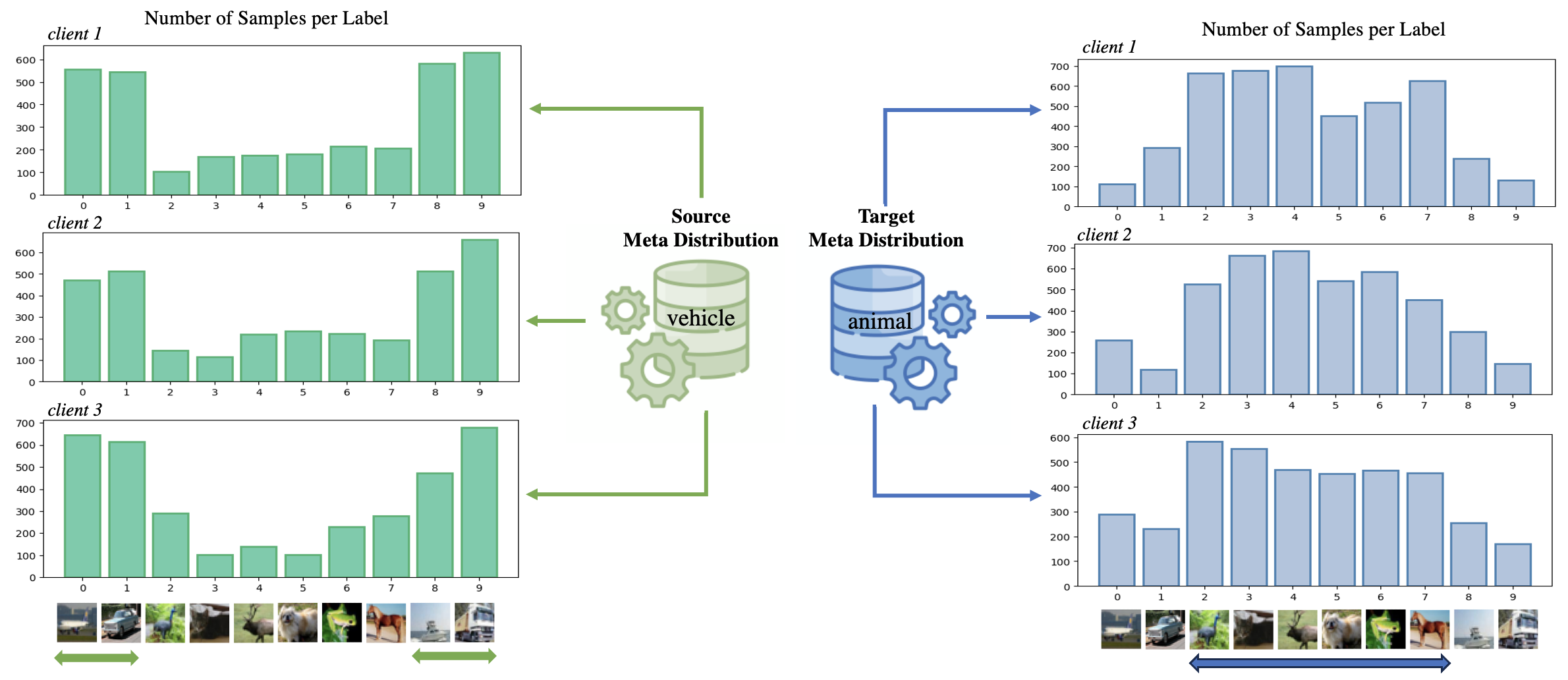
In this work, we focus on evaluating FL models on unseen clients and networks. We assume access to clients whose data distributions are i.i.d. samples from a meta-distribution (an unknown distribution over data distributions), which represents the population of clients (e.g., a mobile network in a specific region). Our goal is to provide performance guarantees for unseen clients whose data either follows the same meta-distribution or a different one within a bounded distance from . The latter corresponds to a different society with slightly different life-styles, habits or preferences (see Figure 1). To address this evaluation challenge, we extend non-asymptotic average loss and/or CDF estimation guarantees to the performance scores collected from observed clients. Specifically, we leverage the Dvoretzky–Kiefer–Wolfowitz (DKW) theorem to provide probably approximately correct (PAC) guarantees for unseen clients following the same meta-distribution [5]. These guarantees offer lower bounds on the performance score of an unseen client with adjustable confidence.
In real-world applications, however, test clients may come from different populations, unseen during training. To account for this, we extend the DKW theorem to cover meta-distributions within a bounded divergence from the source. This extension includes an upper bound on the CDF for meta-distributions within a bounded -divergence. We also give performance guarantees via tightly bounding the meta-distributionally shifted average loss when both -divergence or Wasserstein shifts are considered. The -divergence approach captures potential reweightings of client types in the target network, while the Wasserstein distance models more complicated distributional shifts, such as new clients emerging from previously unseen regions of the distribution’s support (e.g., cultural differences) [24, 9]. To the best of our knowledge, this is the first extension of the DKW bound and the Glivenko-Cantelli theorem to such an adversarially robust setting.
Our bounds are consistent, converging to zero as the number of observed clients, , and the number of data points per client, for , grow asymptotically large. Additionally, we demonstrate that Wasserstein-type meta-distributional shifts can be handled by querying clients for their adversarial loss instead of ordinary loss, a task achievable without direct access to user data. We also show that the number of queries per client can be bounded by a polynomial function of the problem parameters. Finally, we validate the practicality and computational efficiency of our bounds through experiments on well-known real-world datasets.
The paper is organized as follows: Section 1.1 reviews related works, while notations and preliminary definitions are introduced in Section 2. Section 3 formally describes our data generation process, our (rather extreme) privacy concerns and restrictions, and finally the main problem. We give a number of vanilla (non-robust) guarantees on the risk average as well as uniform bounds on its CDF in Section 4. However, the proposed -divergence and Wasserstein-based guarantees are presented in Sections 5 and 6, respectively. Experimental results are shown in Section 7. Finally, Section 8 concludes the paper.
1.1 Previous works
Evaluation and Generalization of models learned by FL algorithms on unseen clients. The challenge of generalizing FL models to unseen clients and distributions has been studied in several related works. [13] introduce a method to address the heterogeneity of client data, focusing on improving the generalization of FL models. Similarly, [15] propose a topology-aware federated learning approach that leverages client relationships to enhance model robustness against out-of-federation data. Also, [28] explore adaptive federated learning techniques to dynamically adjust model parameters based on client data distributions.
Distribution shifts and adversarial robustness in FL. The robustness of FL models against distribution shifts and adversarial attacks has been the focus of several related references. [19] propose a robust federated learning framework to handle affine distribution shifts across clients’ data. Their proposed framework incorporates a Wasserstein-distance-based distribution shift model to account for device-dependent data perturbations. Also, [27] conduct comprehensive evaluations on the adversarial robustness of FL models, proposing the decision boundary-based FL Training algorithm to enhance the the trained model’s robustness. [29] gain insight from the bias-variance decomposition to improve adversarial robustness in FL. Also, [2] propose a robust aggregation method to reduce the effect of adversarial clients.
Performance guarantees in Heterogeneous FL. The heterogeneous nature of FL, where clients have different data distributions has been a topic of great interest in the literature. [6] introduce a personalized federated learning framework based on model-agnostic meta-learning, which provides performance guarantees by optimizing for data distribution heterogeneity. [11] propose a classifier calibration method that adjusts for bias in heterogeneous data, offering improved performance guarantees in non-IID settings. [22] develop FedProto, a framework that leverages prototype learning to improve convergence and robustness under non-convex objectives.. Moreover, [23] propose FedLoRA, which adapts low-rank parameter sharing techniques to mitigate the effects of heterogeneity in personalized federated learning. Also, [4] and [8] introduce group-based customization and local parameter sharing strategies, respectively, to provide fairness and efficiency guarantees for heterogeneous client types and multiple tasks in FL.
2 Notations and Preliminaries
In this paper, vectors are denoted by bold letters (e.g., and ), while scalars are represented by ordinary letters (e.g., and ). For a vector and , let denotes the th coordinate of . For , denotes the set .
Consider two measurable spaces and , referred to as the feature and label spaces, respectively. Typically, we assume for some , while may be for binary classification tasks or in regression problems. In our work, can also be a vector without harming the generality of our results. We define the joint feature-label space as , where denotes the Cartesian product. Let denote the set of all probability measures supported on . Each distribution corresponds to a joint measure over a random feature vector and its associated random label . Also, the expectation operator with respect to a measure is denoted by . We refer to as a meta-distribution over , expressed as , where each sample from is itself a probability measure over . In other words, a meta-distribution is a distribution over distributions supported on . In our work, different samples from represent different domains over .
For simplicity, throughout the paper, we abbreviate as . For any two measures , let denote any given distance or divergence between the two distributions. In Section 5, is chosen as an -divergence for a properly defined function , while in Section 6, is selected as a valid Wasserstein metric. Detailed definitions for these scenarios and the corresponding divergences/metrics will be provided in their respective sections. In this context, let denote an -distributional ambiguity ball for . Mathematically, for any measure :
| (1) |
which represents the set of distributions within distance/divergence from according to . Similarly, meta-distributional ambiguity balls are defined as the set of meta-distributions over (i.e., or distributions over distributions supported on ) within an distance from a base meta-distribution . Mathematically:
| (2) |
Here, the deviation can be any properly defined -divergence between the densities of meta-distributions in or a Wasserstein metric with respect to a well-defined transportation cost defined between measures in . In particular, the transportation cost in the latter case can itself be a Wasserstein metric.
Let represent a hypothesis (e.g., a classifier) that maps the feature space onto the label space 111Even though we have assumed a classification/regression scenario, our work goes beyond this limitation and can be applied to any supervised or unsupervised machine learning task. Additionally, assume a fixed loss function , which assigns a loss value to each pair of actual and predicted labels, and , respectively. The expected loss, or Risk, of a hypothesis with respect to a data-generating model is defined as . Here, could be the true data-generating distribution or an empirical approximation obtained from a dataset. The adversarial risk or loss value for any given classifier , with respect to a base statistical or empirical measure and a robustness radius , is formulated as:
| (3) |
which denotes the worst expected loss over all distributions within the -neighborhood of with respect to . In a similar fashion, the meta-distributionally robust loss of a given classifier with respect to a base meta-distribution is defined as:
| (4) |
The geometry of the ball in can be determined using various application-specific divergences or metrics over . In Section 5, we deal with -divergence balls, while Wasserstein meta-distributional balls (using the ordinary Wasserstein metric as their transportation cost) are utilized in Section 6.
3 Problem Definition
This section presents our problem definition. First, let us begin by formally defining the data generation process, outlining our (rather extreme) privacy constraints, and specifying the query policy that governs communication between clients and the server.
Data Generation and Privacy Constraints:
Consider clients connected to a central server. Each client is associated with a unique and private data distribution model , referred to as the th domain. Let be i.i.d. realizations of an unknown meta-distribution over . However, client does not have direct knowledge of their corresponding domain . Instead, they have access to a dataset of size , which contains i.i.d. samples from , i.e.,
| (5) |
Let denote the empirical version of based on the samples in . It should be noted that server knows the value of , no one knows , and is known only to client .
Next, we outline a procedure for the server to evaluate a given model in a federated and distributionally robust manner. This procedure serves as the foundation for communication between the server and clients throughout the paper.
Server-Client Query Policy:
The server queries each of the clients as follows: it sends a model and a robustness radius to client . In response, the client returns the adversarial loss of around :
| (6) |
The type of distributional ball can be defined using any application-specific divergence or metric over . In this work, we only use the adversarial regime (i.e., ) in Section 6 which focuses on Wasserstein balls to provide certified robustness guarantees against meta-distributional shifts. When the robustness radius is unspecified, the client assumes it is zero, and returns the non-robust loss, i.e., . Each client has a maximum number of queries it will accept from the server, referred to as the query budget.
3.1 Our Problem Setup
In a large network with a central server and clients, assume an unknown meta-distribution , and then consider the data generation process described in the previous part. The server sends a model to the clients and can request a number of robust or non-robust loss values for various robustness radii. The ultimate goal on the server side is to use the query policy described in the previous subsection to provide a meta-distributionally robust upper bound for the average or CDF of the loss of . Mathematically speaking, the objective is to compute an empirical value such that the following bound holds with high probability over the selection of clients and their samples:
| (7) |
where the empirical value can be computed at the server-side efficiently. Here, the generalization gap is expected to vanish as both and increase asymptotically. The geometrical properties of the meta-distributional ambiguity ball can be chosen based on the specific application; in this paper, we consider -divergence and Wasserstein balls.
From an algorithmic perspective, should be determined solely using the server-client query policy, which is reflected in the empirical query values for all , using various robustness radii . The server decides the number of queries for each client and the value of for each query. However, the computational cost of evaluating each query at the client side, as well as the total number of queries per client, should increase at most polynomially with respect to the required precision and other problem parameters.
4 Non-Robust Guarantees on Average Risk and Risk Distribution
Throughout this section we assume that the source and target networks, which are being governed by meta-distributions and , respectively, are the same. In other words, we have . Then, we set out to provide high-probability guarantees on both the average and tail probability of the risk of given model based on query values .
Estimating the average risk (loss) of , denoted as , can be done by calculating the empirical mean of the non-robust empirical query values, for . This is expressed as:
| (8) |
As long as the loss function is measurable and bounded (e.g., let be -bounded such as the 0-1 loss), the empirical mean converges quickly to the true statistical loss as both and increase towards infinity. The following theorem provides a non-asymptotic guarantee on the convergence rate:
Theorem 4.1 (Non-Robust Guarantees on the Average Risk).
Let be a meta-distribution over , and let be a measurable and -bounded loss function. Let be i.i.d. instances of , and let for represent their empirical counterparts, formed using i.i.d. private samples from the -th client. Then, for any , the following bound holds with probability at least :
| (9) |
Proof can be found in Appendix A. Thus, by ignoring poly-logarithmic terms, the empirical means over both the users and the samples from each client converge at a rate of . However, in many practical scenarios, interest may lie more in the tail behavior of the risk rather than its average. Specifically, we may wish to estimate the quantiles of the risk distribution, such as determining the proportion of users experiencing a risk level greater than or equal to some threshold .
In this context, the Glivenko-Cantelli theorem provides strong guarantees on the asymptotic behavior of the worst-case error when estimating a cumulative distribution function (CDF) from a finite number of i.i.d. samples [21]. The theorem states that the -norm of the difference between the true CDF of , denoted by , and its empirical version based on i.i.d. samples, denoted by , almost surely converges to zero as approaches infinity. Mathematically, this is expressed as:
| (10) |
Furthermore, the well-known Dvoretzky-Keifer-Wolfowitz (DKW) theorem provides non-asymptotic bounds for this asymptotic behavior.
Lemma 4.2 (DKW Inequality [5]).
Let be a measurable subset of , and let be any probability measure supported on . Let be i.i.d. samples from . Then, the following bound holds for the -norm of the difference between the empirical and true CDF of :
| (11) |
for any .
The proof of this lemma can be found in the reference. This result allows us to provide uniform convergence guarantees on the tail probability of the loss of , i.e., for any , based on i.i.d. observations of the loss across the network. By “uniform,” we mean that, with high probability over the sampling of the users, the worst deviation between the empirical and statistical tail probability is consistently bounded. Formally, we have the following theorem:
Theorem 4.3 (Non-Robust Guarantees on the Risk CDF).
Assume the same setting as Theorem 4.1. Then, with probability at least over the randomness of the configuration, including the sampling of clients and the local and private datasets inside each client, the following bound holds uniformly for all :
| (12) |
for any .
Proof can be found in Appendix A. A similar uniform bound can be provided for the CDF lower-bound. It should be noted that Theorem 4.3 gives us a principled way to provide certified high-probability guarantees on the tail probability of the risk value (i.e. the probability of observing a risk value higher than or equal to ), for all , solely based on i.i.d. observations. Moreover, the only information that is queried by the server from each client is their non-robust risk for a given model , thus client’s privacy is preserved.
In the subsequent sections, we aim to generalize these results to cases where the target meta-distribution differs from the source in unknown ways. We assume they are close according to either an -divergence or Wasserstein distance. By replacing the average loss per client with their adversarial counterparts, or by adversarially combining the loss values from clients on the server side, we can derive guarantees for unseen networks.
5 -Divergence Meta-Distributional Shifts
In this section, we provide high-probability guarantees for the meta-distributionally robust performance of , focusing on both the average loss and the CDF of the risk, under -divergence-based meta-distributional shifts. -divergence is a powerful tool for modeling variations between two probability measures that share the same support. Before presenting these guarantees, we introduce the following key definitions and assumptions, which are essential for understanding the role of -divergence in the context of meta-distributional shifts.
Definition 5.1 (-Divergence Between Meta-Distributions).
Consider two meta-distributions where is absolutely continuous with respect to . Let be a convex function such that is finite for all , , and (which could be infinite). The -divergence between and is defined as:
| (13) |
Assumption 5.2 (Density Ratio Boundedness).
Assume two meta-distributions where both and are absolutely continuous with respect to each other. For , we say and have a -bounded density ratio if the following condition holds for all :
| (14) |
This boundedness for the density ratios of the meta-distributions and is required for a number of theoretical guarantees and practical algorithms, as it limits how much can deviate from , preventing extreme values that could destabilize learning models or theoretical analyses. At this point, we can define an -Divergence ball in as follows:
Definition 5.3 (Meta-Distributional -Divergence Ball).
For a meta-distribution , a function as defined in Definition 5.1, and , the -divergence ball is defined as the following set of meta-distributions:
| (15) |
This defines a set of meta-distributions that are within a certain “distance” of from a reference meta-distribution in terms of -divergence (However, note that -divergence in general is not a distance). It essentially describes a neighborhood around where the divergence does not exceed , providing a controlled way to manage deviations in distributional shifts.
5.1 Theoretical Guarantees on Robustness of Empirical Average Risk
These definitions and assumptions collectively provide a structured way to handle and analyze distributional shifts using -divergence, ensuring that deviations can be quantified, controlled, and bounded. At this point, we can state our main result in the form of the following theorem:
Theorem 5.4 (Empirical Evaluation of with -Divergence Robustness).
Assume a fixed and unknown meta-distributions , let and , and consider to be a proper convex function (see Definition 5.1). Let be an arbitrarily input model and be any 1-bounded loss function. Assume represent i.i.d. and unknown sample distributions from . Accordingly, let for represent a known (but private) empirical dataset of size consisting of i.i.d. samples from . Define as:
| (16) |
where constants only depend on and . Then, for any , the following bound holds with probability at least :
Proof is given in Appendix B. This theorem provides a robust bound on the expected loss under meta-distributional shifts using . This new empirical quantity is derived from a convex optimization problem, determining an upper bound on the average loss considering the -divergence and the bounded density ratio. With high probability (at least ), the expected loss under any shifted meta-distribution can be bounded by plus a term that decreases with and , reflecting the amount of data/clients. The main advantage of our result is that our generalization gap does not have a non-vanishing -dependent term, unlike many existing bounds. Mathematically speaking, we proved the following for any which are -proximal in the -divergence sense:
| (17) |
where hides logarithmic dependencies. Additionally, any inherent “wellness” or “robustness” of the target model is directly reflected through a low value for . In other words, if results in a low error/loss across the sampled distributions (or their empirical counterparts), remains low as well, regardless of the value of . To the best of our knowledge, conventional bounds do not exhibit this adaptivity.
Remark 5.5 (Asymptotic Minimax Optimality).
A notable fact is that is asymptotically minimax optimal, since when it almost surely becomes the true (statistical) adversarial loss of due to the strong law of large numbers. In other words, for asymptotically large values of the said parameters, the adversarial risk is achievable by a meta-distribution which is the -neighborhood of according to .
Proof of Remark 5.5 is a special case (the asymptotic) version of the proof for Theorem 5.4 which is discussed in Appendix B.
Remark 5.6 (Computational Complexity).
The server-side optimization problem in (16) to determine the value of is convex. Given certain smoothness properties of the function , a standard convex optimization algorithm can approximate within an arbitrary error margin , with polynomial time complexity relative to and . The total query budget is , meaning only one ordinary (non-robust) query per client is required.
The proof is straightforward: the objective function in (16) is linear in the parameters , where , and both constraints are convex due to the convexity of in the -divergence definition. Moreover, our proposed procedure results in minimal privacy leakage of private client data, as only the non-robust loss values of (expressed as query values ) are needed, without requiring access to any private data or model gradients.
5.2 Uniform Robustness of the Empirical Risk Distribution
For the case of -divergence robustness, we show that it is also possible to derive an asymptotically consistent and uniform bound for the risk distribution (CDF) which estimates
, for all , simultaneously. Here, represents the unknown target meta-distribution, which is assumed to be within an -proximity of the source meta-distribution . Note that is also unknown, and our access to it is through i.i.d. empirical realizations , where each is known only to client via a private sample set of size . To achieve this, we first derive a robust version of the uniform convergence bound on empirical CDFs, known as the Dvoretzky-Kiefer-Wolfowitz (DKW) inequality:
Lemma 5.7 (Robust Version of DKW Inequality).
Let and be two probability measures on where is absolutely continuous w.r.t. . Assume for to be i.i.d. samples drawn from . Suppose we have for some and a proper convex function . For , let us define the set as
| (18) |
where constants and depend only on . Then, there exists such that the following uniform bound holds with probability at least :
| (19) |
Proof is given in Appendix B. A direct corollary of Lemma 5.7 is the following robust (again with respect to -divergence adversaries) of the well-known Gilivenko-Cantelli theorem:
Corollary 5.8 (Robust Version of Glivenko-Cantelli Theorem).
Let and be two probability measures on and let be an i.i.d. sequence drawn from . Assume and are absolutely continuous with respect to each other. Additionally, suppose for some and a proper convex function . Then, there exists a non-negative sequence that can depend on , has the following properties:
| (20) |
and also satisfies the following condition:
| (21) |
Corollary 5.8 follows directly from Lemma 5.7. Building on the results from Lemma 5.7 and following a similar approach to the one used in Theorem 5.4, we propose the following theorem, which introduces our uniformly convergent and consistent estimator for the risk distribution (i.e., risk CDF):
Theorem 5.9 (Empirical Evaluation of Risk Distribution with -Divergence Robustness).
Assume the setting described in Theorem 5.4. For any let us define:
| (22) |
where are constants that only depend on and . Then, with probability at least , the following bound holds uniformly over all :
| (23) |
The proof is given in Appendix B. The bound in (23) exhibits the following properties: i) It is forward-shifted with respect to the true CDF, meaning it exhibits a delayed reaction to increasing compared to the true CDF. The maximum delay is on the order of ii) The value of the CDF estimator also deviates from the true estimator by the amount . Consequently, as and tend to infinity, the bound becomes asymptotically tight. iii) The bound holds uniformly over all , similar to the original DKW inequality and its corresponding corollary, the Glivenko-Cantelli theorem.
It should be noted that although a separate maximization problem needs to be solved for each value of , these problems are all convex and can therefore be solved efficiently. Additionally, according to Lemma 5.7, there exists a single such that the bound holds for all . However, since this vector is not known, we must take the supremum over for each separately.
6 Wasserstein Meta-Distributional Shifts
This section addresses the case of Wasserstein meta-distributional shifts from to . Such shifts present significant challenges to our robust model evaluation framework, as the model may encounter entirely unseen regions of the distributional support in the target domain. In practical terms, this implies that users may exhibit data distributions that are entirely novel or even drastically different from those encountered during the training phase on the source network. To mitigate the effect of such domain shifts, as we will show later in this section, server needs to query out-of-domain performance measures from each of the clients.
In this section, we provide theoretical guarantees for the average risk, but not for the entire risk distribution. Addressing the full risk distribution requires a more advanced methodology, which falls beyond the scope of the current paper and hence we defer it to future work. We begin by introducing new definitions related to both standard and meta-distributional Wasserstein metrics, and then present our main result, an analog of Theorem 5.4 for Wasserstein-type shifts.
Definition 6.1 (Wasserstein metric on ).
For any two measures and a lower semi-continuous function , we define the Wasserstein distance between and as
| (24) |
where denotes the set of all couplings between and , i.e., all probability measures in that have fixed and as their respective marginals.
The function is called the transportation cost and in practice, for example in a classification task with , can be chosen as for any . However, is user-defined and can be chosen differently. Wasserstein distance (which is a real metric over ) measures the minimum cost of transforming into or vice versa according to the loss characterized by . Unlike -divergence, Wasserstein distance can stay bounded under support shifts. In fact, it is a powerful tool to model slight support changes between distributions and due to this property is widely used in adversarial robustness research.
In a similar fashion, one can define the Wasserstein distance between any two meta-distributions with respect to any valid transportation cost over the space of measures , such as the ordinary Wasserstein distance.
Definition 6.2 (Wasserstein metric over ).
For any two meta-distributions , and a lower semi-continuous transportation cost , let us define
| (25) |
as the Wasserstein distance between and with respect to distributional transportation cost .
Here, is the set of all couplings (measures in ) with and as their respective marginals. Accordingly, for and , we define the Wasserstein ball of radius around as
where the transportation cost is hidden from formulation for the sake of simplicity. Similarly, one can define the Wasserstein ball around meta-distribution with radius as the set of meta-distributions with a (meta-distributional) Wasserstein distance of at most from as follows:
| (26) |
We now present our main result of this section: a quasi-convex (and thus polynomial-time) optimization problem that provides empirical meta-distributionally robust evaluation guarantees against Wasserstein shifts, with a asymptotically vanishing generalization gap.
Theorem 6.3 (Empirical Evaluation of with Wasserstein Robustness).
Assume an unknown meta-distributions , let be an arbitrarily model and let be a -bounded non-negative loss function. Assume represent i.i.d. and unknown sample distributions from . Accordingly, let for represent a known (but private) empirical dataset of size consisting of i.i.d. samples from . Let be a bounded and proper (according to Definition 6.2) transportation cost on . For any given , consider the following constrained optimization problem:
| (27) |
Then, the following bound holds with probability at least for the meta-distributionally robust loss of around meta-distribution :
| (28) |
where is a universal constant and only depends on transportation cost .
The proof is provided in Appendix C. Similar to Theorem 5.4, Theorem 6.3 offers a robust bound on the expected loss under Wasserstein meta-distributional shifts using . Once again, the generalization gap decreases asymptotically as both and increase. Specifically, we have:
| (29) |
It is important to note that the inherent robustness of against Wasserstein-type distributional shifts, if it exists, would be reflected in , thereby reducing the bound. In the following, we also discuss the computational complexity and privacy aspects of our scheme in Remarks 6.4, 6.5, and 6.6.
Remark 6.4 (Server-side Computational Complexity).
The server-side optimization problem in (27) to determine the value of is quasi-convex. Without any additional requirements or assumptions, a standard quasi-convex optimization algorithm, such as the bisection method described in Algorithm 1 (see Appendix D), can approximate within an arbitrary error margin , with polynomial time complexity relative to and . The total query budget per client is also polynomial with respect to both and .
Remark 6.5 (Client-side Computational Complexity).
Assume the transportation cost in Theorem 6.3 is convex with respect to its second argument222This assumption is generally not restrictive, as any norm exhibits this property and is differentiable. Also, assume the robustness radius is not chosen to be excessively large. Under these conditions, the client-side optimization problem to determine the query value in (27), for any given and , is convex [20]. A standard stochastic gradient descent algorithm can approximate within an arbitrary error margin , with polynomial time complexity relative to , and .
The proof of Remark 6.5 relies on the concavity of the objective function in the adversarial loss value when is not excessively large (equivalently, when in the dual form is sufficiently large). Notably, this property holds regardless of whether is convex. The key factor is the largest absolute eigenvalue of the Hessian of the loss function . In Section 2 of [20], a detailed analysis of the convergence rate for such problems is provided, assuming that the transportation cost is strongly convex with respect to one of its arguments. It is also worth noting that strongly convex transportation costs are widely used in real-world applications and cover a broad range of options, including many valid norms.
Remark 6.6 (Certificate of Privacy).
The optimization problem used to determine the empirical value in (27) relies solely on the Wasserstein adversarial loss values from each client , derived using the query value for polynomially many values of . No other information or direct access to private client data is required. To the best of our knowledge, there are no known privacy attacks capable of effectively recovering private data from this procedure.
7 Experimental Results
In this section, we present a series of experiments on real-world datasets to demonstrate both: (i) the validity and tightness of our bounds, and (ii) that our bounds are not only theoretically sound but also computable in practice.
7.1 Client Generation and Risk CDF Certificates for Unseen Clients
In the first part of our experiments, we outline our client generation model and present a number of risk CDF guarantees. We simulated a federated learning scenario with nodes, where each node contains local samples. The experiments were conducted using four different datasets: CIFAR-10 [10], SVHN [17], EMNIST [3], and ImageNet [18]. To create each user’s data within the network, we applied three types of affine distribution shifts across users:
-
•
Feature Distribution Shift: Each sample in the dataset is manipulated via a transformation chosen randomly for each node. Specifically, each user is assigned a unique matrix and shift vector , and the data is modified as follows:
(30) In our experiments, and are respectively random matrices and vectors with i.i.d. zero-mean Gaussian entries. The standard deviation varies based on the dataset: for CIFAR-10 and SVHN, for EMNIST, and for ImageNet.
-
•
Label Distribution Shift: Here, we assume that each meta-distribution is characterized by a specific coefficient. To generate each user’s data under this shift, the number of samples per class is determined by a Dirichlet distribution with parameter . In our experiments, we use .
-
•
Feature & Label Distribution Shift: As the name suggests, this shift combines both the feature and label distribution shifts described above to create a new distribution for each user.
Figure 2 illustrates our performance certificates (i.e., bounds on the risk CDF) for unseen clients when there are no shifts. We selected nodes from the population and considered other nodes as unseen clients. We then plotted the CDFs based on samples and confirmed that our bounds hold for the real population as well. Due to the standard DKW inequality, the empirical CDF is a good estimate for the test-time non-robust risk CDF.
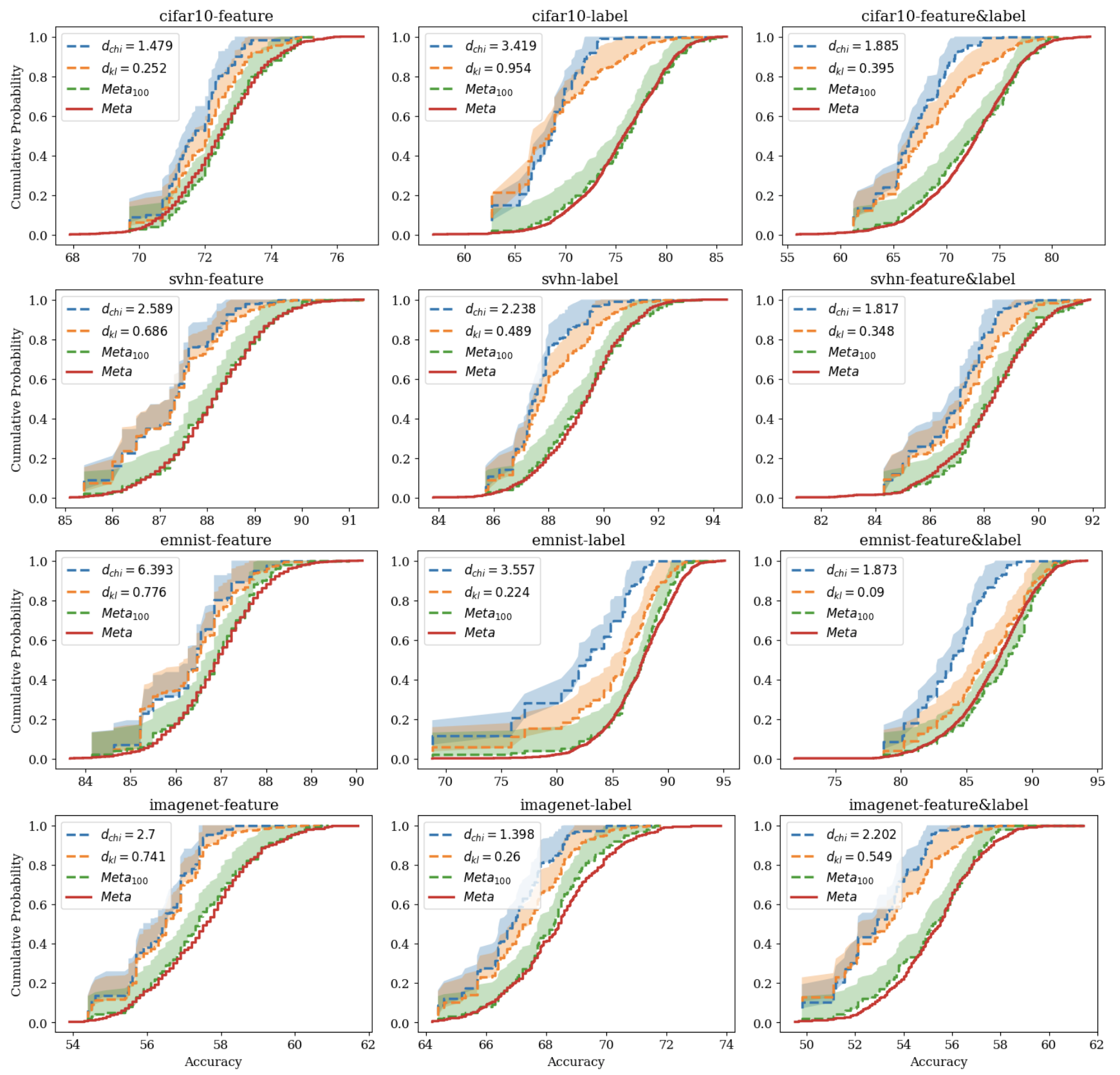
7.2 Certificates for -Divergence Meta-Distributional Shifts
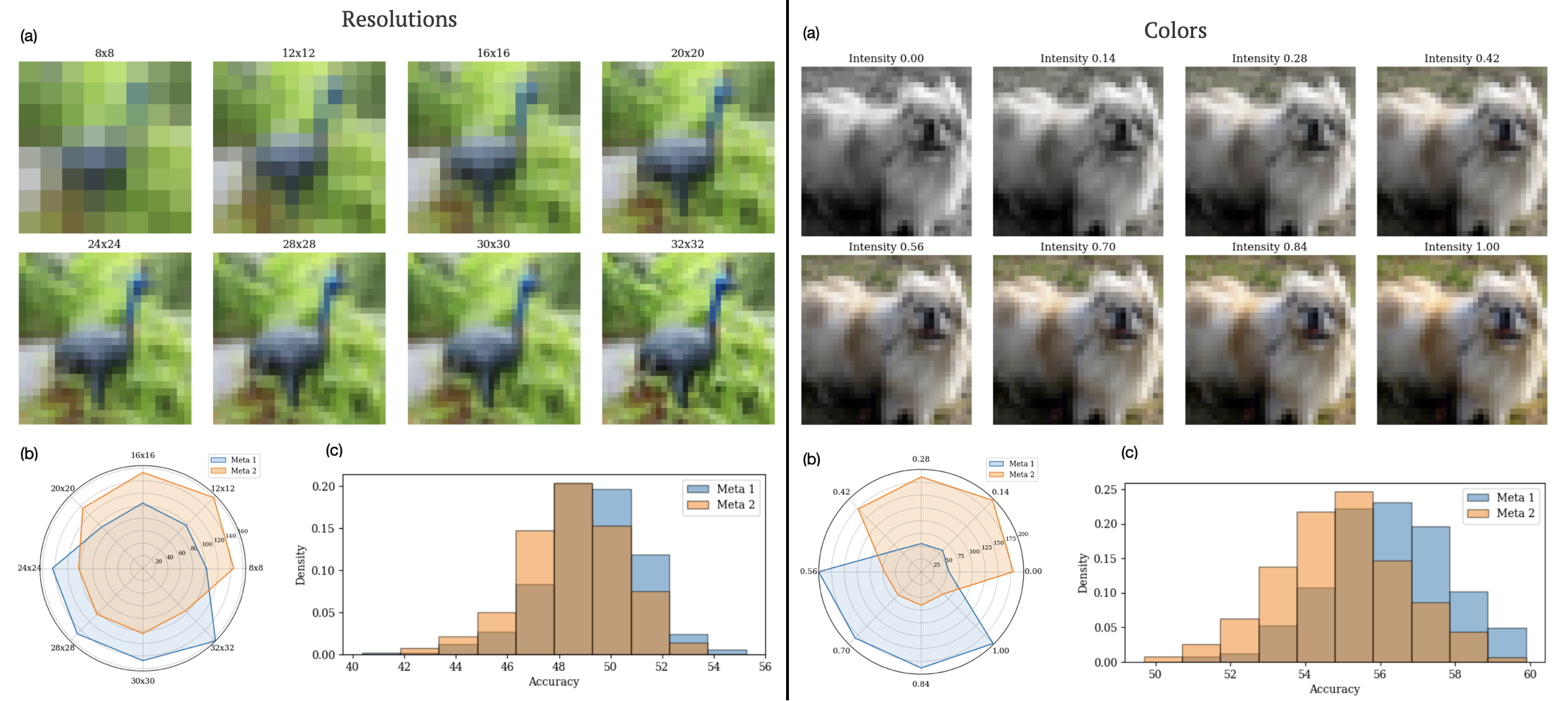
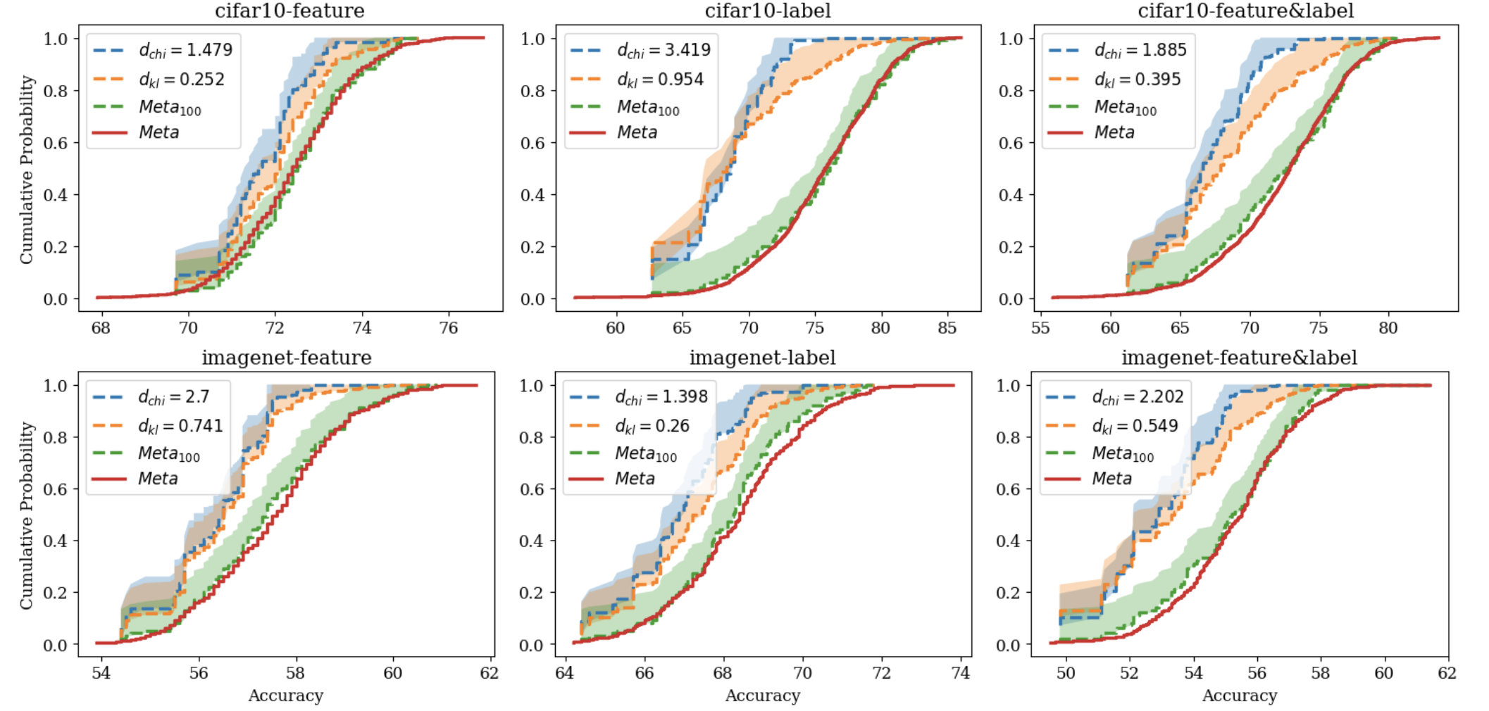
In this section, we examined scenarios where users belong to two distinct meta-distributions: the source and the target. A DNN-based model is initially trained on a network of clients sampled from the source. The resulting risk values are then fed into the optimization problems introduced in Section 5 to obtain robust CDF bounds, considering both the Chi-Square and KL divergence as potential choices for . Finally, we empirically estimate the risk CDF for users from the target meta-distribution and validate our bounds. Specifically, we tested our certificates in two distinct settings using the CIFAR-10 dataset (see Figure 3). We generated various image categories with differing resolutions or color schemes, and then sampled from these categories to create different distributions:
-
•
Resolutions: Images were cropped and resized to create eight different resolutions. The Dirichlet coefficients for the first (source) meta-distribution range from to for the four lower resolutions and from to for the four higher resolutions. For the second (target) meta-distribution, the ranges are reversed: to for the lower resolutions and to for the higher resolutions. The number of samples per resolution for each user is determined using a Dirichlet distribution, with coefficients randomly selected from the specified range for the meta-distribution. As a result, users sampled from source will have more high-resolution images, while users from the target will have more low-resolution samples.
-
•
Colors: The color intensity of the images varies from (gray-scale) to (fully colored). For the source meta-distribution, the coefficients range from to for images with color intensity below , and from to for images above . As with the resolution setting, the ranges are reversed for the target, and the number of samples per color intensity for each user is calculated similarly. Therefore, users sampled from source will have more colorful images, while those from the target will have more gray-scale images.
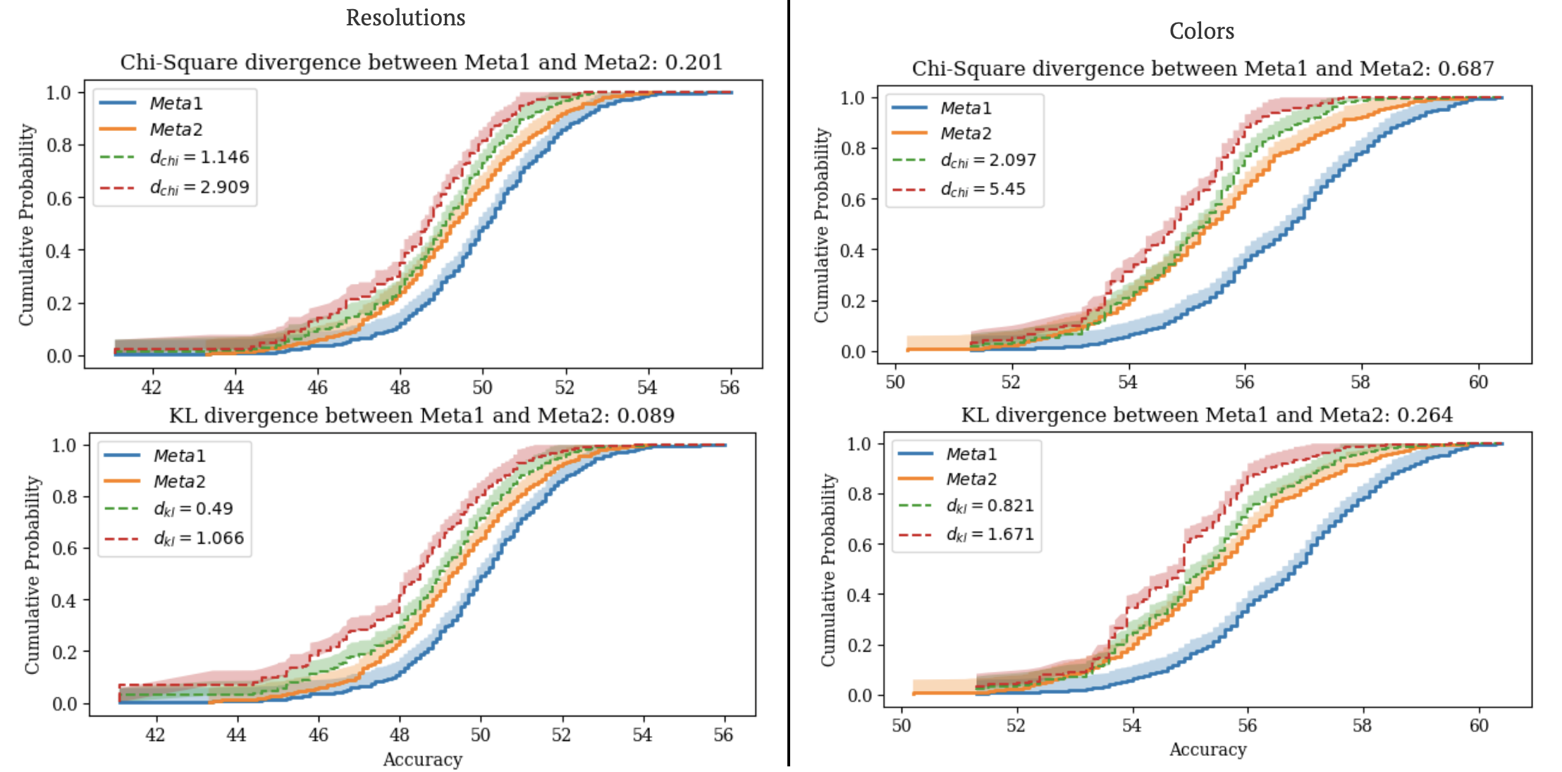
Figure 4 (left) verifies our CDF certificates based on both chi-square and KL-divergence (dotted curves) for the target meta distribution (orange curve). As can be seen, bounds have tightly captured the behavior of risk CDF in the target network. More detailed experiments are shown in Figure 6 in Appendix E.
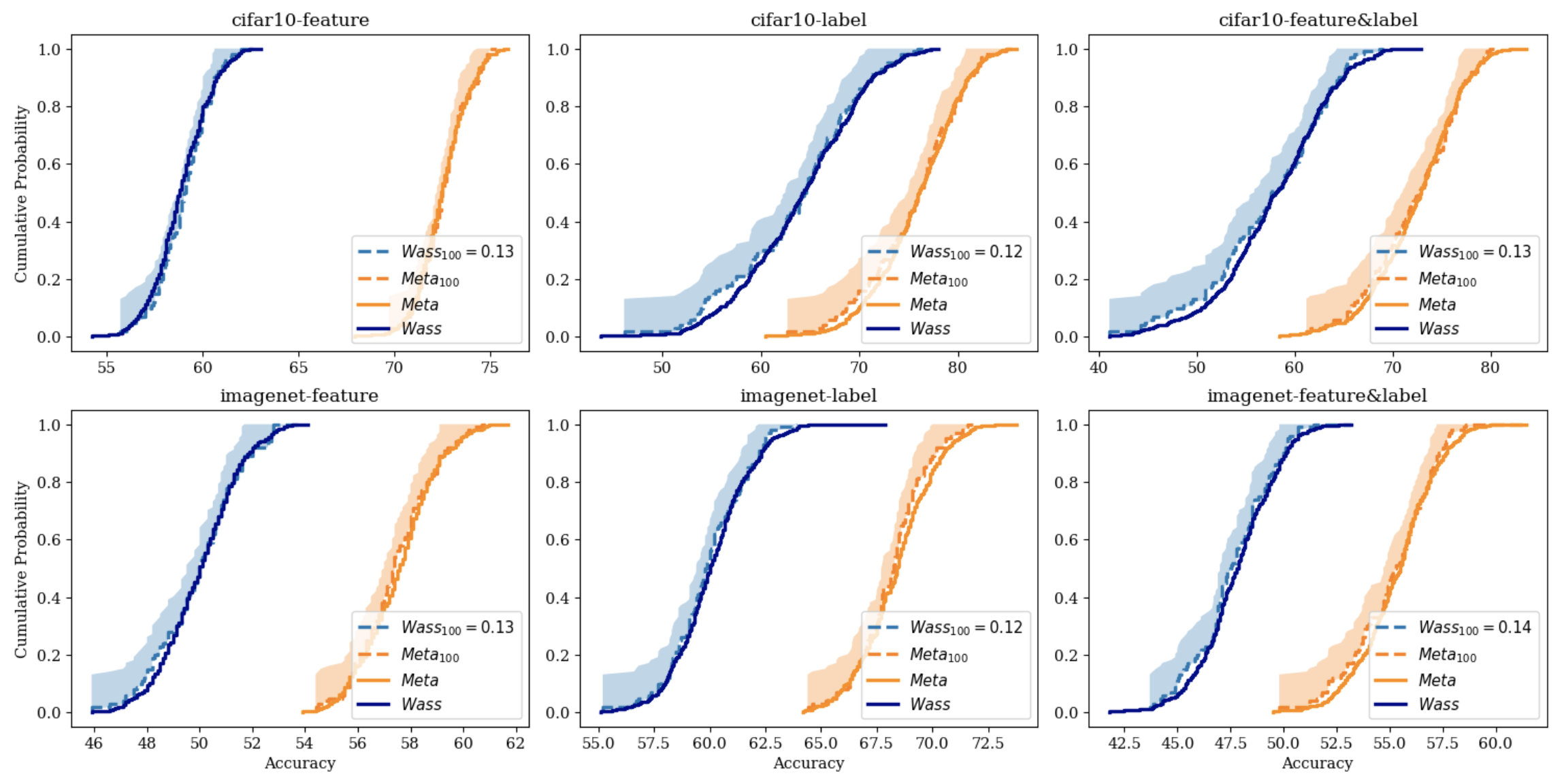
7.3 Certificates for Wasserstein-based Meta-Distributional Shifts
In this experiment, as previously mentioned, we used affine distribution shifts to create new domains. Figure 4 (right) summarizes our numerical results in this scenario. To generate different networks within the meta-distribution, we applied the affine distribution shifts described in Section 7.1. Once again, the results validate our certificates, this time for Wasserstein-type shifts. The blue curve, representing the real population, consistently falls within or beneath the blue shaded area. Regarding tightness, it is important to note that the bounds presented here remain tight, particularly under adversarial attacks as defined by a distributional adversary in [20]. More detailed experiments with various levels of tightness are shown in Figure 7 in Appendix E.
Although our theoretical findings in Section 6 focus solely on the average risk and not the risk CDF, we extended the same framework to the CDF in this experiment to explore whether the theory might also apply. The results were positive, suggesting potential for extending our theoretical findings in this area.
8 Conclusions
In this work, we proposed a series of new performance bounds, all computable in polynomial time with (at worst) polynomial query complexity, to establish performance guarantees for any given model (e.g., a classifier) on an unseen network B, based solely on observations and query results from network A. The key assumption is that the meta-distributions governing the user data distributions in both networks are -close, for some known or assumed . The notion of “closeness” plays a critical role, and we considered two broadly used measures for this purpose: -divergence shifts and Wasserstein shifts. These shifts capture different practical scenarios, making our approach applicable to a wide range of use cases.
Our bounds are supported by rigorous mathematical proofs, detailed in the Appendix. They exhibit vanishing generalization gaps, ensuring consistency as the network size and the network-normalized sample per client increase asymptotically. Notably, we introduced a robust version of the well-known GC theorem and DKW bound specifically for -divergence shifts, which, to the best of our knowledge, is entirely novel.
Our numerical experiments demonstrate the practical effectiveness of our bounds in terms of both tightness and computability, as all of our proposed optimization problems are convex or quasi-convex and thus solvable in polynomial time. For future work, one could focus on deriving similar uniform convergence bounds for the risk CDF under Wasserstein-type meta-distributional shifts. Additionally, exploring other types of shifts beyond -divergence and Wasserstein could be a promising direction.
References
- BM [19] Jose Blanchet and Karthyek Murthy. Quantifying distributional model risk via optimal transport. Mathematics of Operations Research, 44(2):565–600, 2019.
- BMCDN [22] Adnan Ben Mansour, Gaia Carenini, Alexandre Duplessis, and David Naccache. Federated learning aggregation: New robust algorithms with guarantees. arXiv preprint arXiv:2205.10864, 2022.
- CATVS [17] Gregory Cohen, Saeed Afshar, Jonathan Tapson, and Andre Van Schaik. Emnist: Extending mnist to handwritten letters. In 2017 international joint conference on neural networks (IJCNN), pages 2921–2926. IEEE, 2017.
- CYC+ [24] Shu-Ling Cheng, Chin-Yuan Yeh, Ting-An Chen, Eliana Pastor, and Ming-Syan Chen. Fedgcr: Achieving performance and fairness for federated learning with distinct client types via group customization and reweighting. In Proceedings of the 38th AAAI Conference on Artificial Intelligence (AAAI), 2024.
- DKW [56] Aryeh Dvoretzky, Jack Kiefer, and Jacob Wolfowitz. Asymptotic minimax character of the sample distribution function and of the classical multinomial estimator. The Annals of Mathematical Statistics, pages 642–669, 1956.
- FMO [20] Alireza Fallah, Aryan Mokhtari, and Asuman Ozdaglar. Personalized federated learning with theoretical guarantees: A model-agnostic meta-learning approach. In Advances in Neural Information Processing Systems 33 (NeurIPS), 2020.
- GI [89] Peter W Glynn and Donald L Iglehart. Importance sampling for stochastic simulations. Management science, 35(11):1367–1392, 1989.
- JZBD [24] Yongzhe Jia, Xuyun Zhang, Amin Beheshti, and Wanchun Dou. Fedlps: Heterogeneous federated learning for multiple tasks with local parameter sharing. In Proceedings of the 38th AAAI Conference on Artificial Intelligence (AAAI), 2024.
- KENSA [19] Daniel Kuhn, Peyman Mohajerin Esfahani, Viet Anh Nguyen, and Soroosh Shafieezadeh-Abadeh. Wasserstein distributionally robust optimization: Theory and applications in machine learning. In Operations research & management science in the age of analytics, pages 130–166. Informs, 2019.
- KH+ [09] Alex Krizhevsky, Geoffrey Hinton, et al. Learning multiple layers of features from tiny images. Technical report, University of Toronto, 2009.
- LCH+ [21] Mi Luo, Fei Chen, Dapeng Hu, Yifan Zhang, Jian Liang, and Jiashi Feng. No fear of heterogeneity: Classifier calibration for federated learning with non-iid data. In Advances in Neural Information Processing Systems 34 (NeurIPS), 2021.
- LLGL [24] Bingyan Liu, Nuoyan Lv, Yuanchun Guo, and Yawen Li. Recent advances on federated learning: A systematic survey. Neurocomputing, page 128019, 2024.
- LSTS [20] Tian Li, Anit Kumar Sahu, Ameet Talwalkar, and Virginia Smith. Federated learning with matched averaging. In Proceedings of the 34th Conference on Neural Information Processing Systems (NeurIPS), 2020.
- M+ [89] Colin McDiarmid et al. On the method of bounded differences. Surveys in combinatorics, 141(1):148–188, 1989.
- MLP [24] Mengmeng Ma, Tang Li, and Xi Peng. Beyond the federation: Topology-aware federated learning for generalization to unseen clients. In Ruslan Salakhutdinov, Zico Kolter, Katherine Heller, Adrian Weller, Nuria Oliver, Jonathan Scarlett, and Felix Berkenkamp, editors, Proceedings of the 41st International Conference on Machine Learning, volume 235 of Proceedings of Machine Learning Research, pages 33794–33810. PMLR, 21–27 Jul 2024.
- MMR+ [17] Brendan McMahan, Eider Moore, Daniel Ramage, Seth Hampson, and Blaise Aguera y Arcas. Communication-efficient learning of deep networks from decentralized data. In Artificial intelligence and statistics, pages 1273–1282. PMLR, 2017.
- NWC+ [11] Yuval Netzer, Tao Wang, Adam Coates, Alessandro Bissacco, Baolin Wu, Andrew Y Ng, et al. Reading digits in natural images with unsupervised feature learning. In NIPS workshop on deep learning and unsupervised feature learning, volume 2011, page 4. Granada, 2011.
- RDS+ [15] Olga Russakovsky, Jia Deng, Hao Su, Jonathan Krause, Sanjeev Satheesh, Sean Ma, Zhiheng Huang, Andrej Karpathy, Aditya Khosla, Michael Bernstein, et al. Imagenet large scale visual recognition challenge. International journal of computer vision, 115:211–252, 2015.
- RFPJ [20] Amirhossein Reisizadeh, Farzan Farnia, Ramtin Pedarsani, and Ali Jadbabaie. Robust federated learning: The case of affine distribution shifts. Advances in Neural Information Processing Systems, 33:21554–21565, 2020.
- SND [18] Aman Sinha, Hongseok Namkoong, and John Duchi. Certifying some distributional robustness with principled adversarial training. In International Conference on Learning Representations, 2018.
- Tal [87] Michel Talagrand. The glivenko-cantelli problem. The Annals of Probability, pages 837–870, 1987.
- TLL+ [22] Yue Tan, Guodong Long, Lu Liu, Tianyi Zhou, Qinghua Lu, Jing Jiang, and Chengqi Zhang. Fedproto: Federated prototype learning across heterogeneous clients. In Proceedings of the 36th AAAI Conference on Artificial Intelligence (AAAI), 2022.
- WLN+ [24] Xinghao Wu, Xuefeng Liu, Jianwei Niu, Haolin Wang, Shaojie Tang, and Guogang Zhu. Fedlora: When personalized federated learning meets low-rank adaptation. In International Conference on Learning Representations (ICLR), 2024.
- WWS+ [22] Zhenyi Wang, Xiaoyang Wang, Li Shen, Qiuling Suo, Kaiqiang Song, Dong Yu, Yan Shen, and Mingchen Gao. Meta-learning without data via wasserstein distributionally-robust model fusion. In Uncertainty in Artificial Intelligence, pages 2045–2055. PMLR, 2022.
- YFD+ [23] Mang Ye, Xiuwen Fang, Bo Du, Pong C Yuen, and Dacheng Tao. Heterogeneous federated learning: State-of-the-art and research challenges. ACM Computing Surveys, 56(3):1–44, 2023.
- ZAC+ [21] Syed Zawad, Ahsan Ali, Pin-Yu Chen, Ali Anwar, Yi Zhou, Nathalie Baracaldo, Yuan Tian, and Feng Yan. Curse or redemption? how data heterogeneity affects the robustness of federated learning. In Proceedings of the AAAI conference on artificial intelligence, volume 35, pages 10807–10814, 2021.
- ZLC+ [23] Jie Zhang, Bo Li, Chen Chen, Lingjuan Lyu, Shuang Wu, Shouhong Ding, and Chao Wu. Delving into the adversarial robustness of federated learning. In Proceedings of the AAAI Conference on Artificial Intelligence, 2023.
- ZMY+ [23] Yan Zeng, Yuankai Mu, Junfeng Yuan, Siyuan Teng, Jilin Zhang, Jian Wan, Yongjian Ren, and Yunquan Zhang. Adaptive federated learning with non-iid data. The Computer Journal, 66(11):2758–2772, 2023.
- ZWWH [22] Yao Zhou, Jun Wu, Haixun Wang, and Jingrui He. Adversarial robustness through bias variance decomposition: A new perspective for federated learning. arXiv preprint arXiv:2009.09026, 2022.
- ZYG [24] Luhao Zhang, Jincheng Yang, and Rui Gao. A short and general duality proof for wasserstein distributionally robust optimization. Operations Research, 2024.
Appendix A Proofs of the Statements in Section 4
Proof of Theorem 4.1.
The proof is straightforward and combines several applications of McDiarmid’s inequality (or, more simply in this case, Hoeffding’s inequality). For any instance of distributions , let us define the random variable as follows:
| (31) |
where denotes the loss function, and is the space of possible outcomes. We omit the detailed proof that being a random variable implies is also a random variable, as this follows from standard measurability arguments.
Now, for any , we apply McDiarmid’s inequality to obtain:
| (32) |
where the bound holds due to the one-sided version of McDiarmid’s inequality, and the fact that almost surely.
Next, for each , we similarly have:
| (33) |
This follows from Hoeffding’s inequality, given that the data points in the local dataset of the -th client are i.i.d. By the union bound, the above inequalities hold simultaneously with probability at least . Finally, combining these inequalities gives us the desired bound in the theorem, thus completing the proof. ∎
Proof of Theorem 4.3.
Proof follows the same path as the one paved during the proof of Theorem 4.1. Let us define the statistical query value of the th client as , i.e.,
| (34) |
where is the true (unknown) data generating distribution which is assigned to client . In this regard, according to Lemma 4.2, for any we have
Also, applying the McDiarmid’s inequality for times (once, with respect to each client ), the following bounds also hold:
| (35) |
which show the boundedness of the deviation between the empirical query values and statistical ones . This is similar to the proof of Theorem 4.1. Again, applying union bound and combining all the inequalities mentioned so far in the proof, the final bound in the statement of the theorem holds with probability at least and the proof is complete. ∎
Appendix B Proofs of the Statements in Section 5
Proof of Theorem 5.4.
For each , let us define the event as follows:
| (36) |
where, since is assumed to be a 1-bounded loss function and the samples are drawn independently, McDiarmid’s inequality tells us that [14]. We now state and prove two essential lemmas which will be used in the subsequent arguments.
Lemma B.1.
Consider two meta-distributions which are absolutely continuous with respect to each other and have a -bounded density ratio for some . For , assume to be i.i.d. sample distributions sampled from . Then, for all , the following concentration bound holds:
| (37) |
Proof of Lemma B.1.
Due to the assumed mutual absolute continuity, and share the same support. Therefore, for , we can define the scalar random variable
| (38) |
This variable is bounded by . Regarding the expected value of , we have:
| (39) |
Let . Since represent i.i.d. instances of , McDiarmid’s inequality states that:
| (40) |
which completes the proof. ∎
Lemma B.2.
For , assume two meta-distributions are absolutely continuous with respect to each other and have a -bounded density ratio. Let be a convex function that satisfies the conditions described in Definition 5.1. For , assume to be i.i.d. sample distributions sampled from . Then, the following concentration bound holds:
| (41) |
where is defined as:
| (42) |
Proof of Lemma B.2.
The proof follows similarly to that of Lemma B.1. For , let us define the random variable
| (43) |
Then, having defined , we know that represent i.i.d. instances of . Moreover, the expected value of is the -divergence between and :
| (44) |
Finally, since and have the -bounded density ratio property, the following bounds hold almost surely:
| (45) |
which means the range of is almost surely equal to . Hence, again using McDiarmid’s inequality, we get the bound:
| (46) |
and this completes the proof. ∎
With the lemmas established, let us define additional events and based on the concentration bounds:
| (47) | ||||
| (48) |
where are constants which only depend on and , according to Lemmas B.1 and B.2. Based on the above arguments and the results of the mentioned lemmas, we have . Using the central idea for importance sampling [7], the following equations hold for all and :
| (49) |
At this point, and similar to the idea of Lemma B.1, we define as the event of the empirical loss over meta-distribution concentrates (with high probability) around its expected value, i.e.,
| (50) |
Again, since
McDiarmid’s inequality states that the probability bound holds. Our final definition in this proof is a random set of meta-distributions which represents an empirical candidate for the neighbors of . Mathematically speaking, let us define:
| (51) |
which depends on and has a random (empirical) nature since it also depends on sample distributions . Based on prior discussions and lemmas, we have as long as the events and hold, simultaneously. By further assuming that events and s for all also hold, we can finally write the following chain of inequalities:
| (52) | |||
It should be noted that the condition can be interpreted as introducing
and force to satisfy the constraints in the definition of . Hence, this gives us the high probability bound claimed inside the statement of theorem. The only remaining part of the proof is to show events and for all hold, simultaneously, with a probability at least .
For any event , let denote its complement. Then, we already have
In this regard, one can simply use the union bound and obtain the following chain of inequalities:
| (53) |
This means the bound in the statement of theorem holds with a probability at least , and thus completes the proof. ∎
Proof of Lemma 5.7.
The proof for most of its initial parts follows the same path as in the proof of Theorem 5.4. In particular, we use Lemmas B.1 and B.2 from the proof of Theorem 5.4 to show that the following events occur separately with probability at least , for any :
| (54) | |||
| (55) |
where are constants depending on . These probabilities are with respect to the randomness in drawing i.i.d. samples . This is equivalent to the following statement:
| (56) |
Next, define for as
| (57) |
where the weight function is the unknown (bounded) density ratio between and , i.e.,
| (58) |
Since is non-negative, is non-decreasing in , starting at when and not exceeding as .
Consider the probability measure . For , define such that (i) and , and (ii) for . These represent the -quantiles of . For any , let be such that . Then, the following chain of inequalities holds almost surely for all :
| (59) |
Thus, the following bound holds for all :
| (60) |
On the other hand, for any fixed , we have the following relation for the expectation of :
| (61) |
Given that the weight functions for are bounded in the interval , and , McDiarmid’s inequality states that for any ,
| (62) |
Therefore, using the union bound over all , we obtain:
| (63) |
Equivalently, for any , the following bound holds with probability at least :
| (64) |
Using the preceding inequalities, in particular relations in (56), (60) and (64), we can say there exists such that the following bounds for hold with probability at least :
| (65) |
Thus, the proof is complete. ∎
Proof of Theorem 5.9.
Similar to the proof of Theorem 5.4, we begin by noting that, due to McDiarmid’s inequality, for any , with probability at least , the following set of inequalities holds simultaneously for all :
| (66) |
Next, it can be readily verified that:
| (67) |
Additionally, note that:
| (68) |
The remainder of the proof simply involves applying the result of Lemma 5.7 with a maximum error probability of . This concludes the proof. ∎
Appendix C Proofs of the Statements in Section 6
Proof of Theorem 6.3.
Proof consists of two parts:
-
•
Proving the statement of theorem for the statistical case, where and thus we have for all , and .
-
•
Replacing the statistically exact adversarial loss which is based on the unknown distribution sample with its empirically calculated counterpart which is computed based on the known (yet private) distribution for all . This part of the proof requires establishing a uniform convergence bound over all values of .
Part I
The core mathematical tool used throughout the proof is the following duality result from [20] (originally derived in [1]) which works for general Wasserstein-constrained optimization problems:
Lemma C.1 (Proposition 1 of [20]).
Let be a probability measure defined over a measurable space , be any loss function, denote a proper and lower semi-continuous transportation cost on , and assume . Then, the following equality holds for the Wasserstein-constrained DRO around :
| (69) |
Proof can be found inside the reference. Also, [1] and [30] along with several other papers have theoretically analyzed alternative proofs. Based on the duality formulation in Lemma C.1, and considering the fact that meta-distribution is also a “distribution” over the measurable space , one can rewrite the original Wasserstein-constrained MDRO in the statement of the theorem in its dual form:
| (70) |
The main advantage achieved by this reformulation is the substitution of with the fixed meta-distribution inside the expectation operators. Therefore, the optimization no longer has to be carried out in the space. For the sake of simplicity in the proof, assume supreme value in (70) is attainable. This assumption is not necessary, and can be relaxed by using a more detailed mathematical analysis which is replacing the optimal distribution with a Cauchy series of distributions and proceed with similar arguments. However, we have decided to avoid this scenario in order to simplify the proof. In this regard, let us define:
| (71) |
Then, the following relation holds:
| (72) |
which, can be simply rewritten as:
| (73) |
Using a similar argument as before, let us assume the in (73) is also attainable and denote the optimal value by . Once again, this assumption is not necessary and can be relaxed at the expense of introducing more mathematical details and making the proof less readable. In this regard, we have:
| (74) |
where it has been already guaranteed that the optimal parameter and optimal distribution , the following constraint holds:
| (75) |
For any , let us define the following optimal robustness radius function
| (76) |
Therefore, the original MDRO objective in the statement of the theorem can be readily upper-bounded using the following distributionally robust formulation:
| (77) |
Using the upper-bound in (77) and the inequality condition on optimal Wasserstein radius functions described in (75), we can proceed to the empirical stage of the proof. At this stage, the true expectation operators should be replaced by their empirical counterparts which are based on i.i.d. realizations of meta-distribution , i.e., unknown distributions and their known yet private empirical realizations, i.e., for .
For , let us define the following new and real-valued random variables and as follows:
| (78) |
It should be noted that is readily known to be (almost surely) bounded by , since is assumed to be -bounded. Additionally, the boundedness for directly results from the assumption that is a bounded transportation cost.
Lemma C.2.
There exists such that We have for .
Proof.
The proof is straightforward and directly results from the definition of Wasserstein distance:
| (79) |
which concludes the proof. ∎
Using a similar series of arguments to the ones explained in Lemmas B.1 and B.2 (proof of Theorem 5.4), together with the fact that s are all bounded by , one can directly apply the McDiarmid’s inequality and show that the following bound holds with probability at least , for any :
| (80) |
On the other hand, by using the boundedness property for proved in Lemma C.2 and applying McDiarmid’s inequality once again, the following bound holds with probability (for any ) for the empirical mean of over true sample distributions :
| (81) |
where is a known universal constant depending only on the bound on transportation cost . Here, the last inequality is a direct consequence of the property shown in (75).
Let be defined as the following subset:
| (82) |
So far, we have shown that
| (83) |
In a similar procedure to the one used in the proof of Theorem 5.4, union bound ensures that the bound in (80) and the mathematical statement of simultaneously hold with probability at least . Then the following chain of bounds also hold with the same probability w.r.t. drawing of from :
| (84) |
For reasons that become clear in the final stages of the proof, we need to replace the set with a new one denoted by which should be defined as:
Evidently, replacing with in the maximization step of (84), i.e., , gives an upper bound for the original formulation of , since each member of can be formed by taking a member from and add all radius values by a constant . Obviously, this procedure only makes the adversarial loss value larger and hence all the bounds still apply.
Part II:
So far, we have managed to (partially) prove the proposed bound in the statement of the theorem in scenarios where and thus we have for all . At this stage of the proof we focus on replacing
for any and arbitrary , with its empirical version . Let us reiterate that we do not have any knowledge regarding , and only client has access to its empirical version which is based on i.i.d. samples. Therefore, is computable via the querying policy described in Section 3, while the true query value is always unknown.
To this aim, similar to [20] first let us define the following function for and :
| (85) |
where is the original transportation cost and abbreviates where we have omitted for simplicity in notation. First, it can readily verified that if is bounded between and , so does for any . Second, note that from Lemma C.1 we have the following duality formulation for and for any :
| (86) | ||||
In the following, first we show that , for any is a Lipschitz function with respect to where the Lipschitz constant only depends on the way the transportation cost is bounded, i.e., the inherent boundedness of or the compactness of . Additionally, we show that the optimal in both minimization problems on the right-hand sides of (86) is bounded by a known constant. The latter result is deduced from the fact that all robustness radii in the statement of theorem has a known margin from zero. Finally, we show the above-mentioned properties can guarantee that uniformly converges to its true expected value for all relevant value of . Hence, the empirical and statistical query values are always within a controlled and asymptotically small deviation from each other regardless of the robustness radius value .
In this regard, the following lemma shows that for any is a Lipschitz function with respect to :
Lemma C.3.
There exists a constant which only depends on transportation cost such that function is -Lipschitz with respect to , for all .
Proof.
For any two distinct values , let and denote the optimal values for which the in (85) is attained. Similar to several previous arguments, attainability of the in this case is not necessary again, and thus this assumption is made for the sake of simplifying the proof.
Then, for any we have:
| (87) | ||||
which directly gives us the following bound:
| (88) |
Through a set of similar arguments and replacing and , the following complementary bound can be achieved as well:
| (89) |
Therefore, the following inequality can be established according to the boundedness of (or alternatively, compactness of ):
| (90) |
which proves the Lipschitz-ness of with respect to . ∎
The following lemma shows that optimal values of in the right-hand side minimization of (86) (or the infimum-achieving sequence in case the infimum is not attainable) is bounded by a known constant:
Lemma C.4.
In both minimization problems on the right-hand side of (86), the optimal value denoted by (if attained), or the tail of its sequence in case the is not attainable, satisfies .
Proof.
Proof directly results from the fact that is bounded between and . Therefore, looking at the dual optimization problem in (86), increasing beyond results in while the second term (i.e., the adversarial loss) is always lower-bounded by zero which makes the whole objective to become larger than . On the other hand, setting would (at worst) results in the objective to be . Therefore, the optimizer should not choose a value that is larger than . ∎
At this point, we can state the main lemma in the second part of the proof, which theoretically shows that empirical query values, i.e., for any fixed and uniformly all converge to their true statistical expected values with a high probability.
Lemma C.5 (Uniform Convergence of Empirical Queries).
For , assume the unknown sample distribution and let for denote i.i.d. feature-label pairs drawn from . The th dataset is only known to client . Then, for any fixed classifier and any , the following bound holds with probability at least :
| (91) |
Proof.
Using the dual formulation of Lemma C.1, we can rewrite the main objective of the theorem as follows:
| (92) |
Again, for the sake of simplicity in the proof let us assume both optimal values and in the minimization problems on the right-hand side of (92) are attainable. It should be noted that this assumption is not necessary and can be relaxed by adding more mathematical work. Then, from Lemma C.4 we already know
Let us partition the feasible search set of , i.e., into equal intervals, where is a small constant which should to be determined later in the proof. For each interval, let us choose a representative (for example, the value at the beginning of the interval) denoted by with . Then, based on Lemma C.3, for any , any corresponding and all we have
| (93) |
where . On the other hand, from the maximization problem that defines in (27), we have that
| (94) |
where we have omitted constants for the sake of readability. Therefore, the above discussions directly lead to the following bound in the statistical sense (i.e., with respect to ):
| (95) |
Through a similar procedure, the following bound also holds for the empirical case (i.e., ), but this time almost surely:
| (96) |
Therefore, according to the fact that is an empirical estimate of based on i.i.d. samples , we have:
| (97) |
Since for each is a non-negative and -bounded (adversarial) loss function, simply applying McDiarmid’s inequality and the union bound over all values of s would give us the following bound which holds with probability at least for any :
| (98) |
which gives us the following bound for with the same high probability:
| (99) |
where function is defined as
It should be noted that is a constant that does not depend on other parameters. Also, we have minimized over since the bound holds irrespective of . Exact solution of the minimization problem in (99) is not needed, since choosing gives us the following bound:
| (100) |
and completes the proof. ∎
By using the uniform convergence result from Lemma C.5 and applying it to all clients simultaneously, we see that (via a union bound argument) with probability at least the empirical and statistical queries and are asymptotically close for all , and uniformly for all robustness radii
which are considered for the maximization problem of (27). Finally, using another union bound argument to incorporate the bounds from (80) and (83) in addition to the previous events, we can say that with probability at least the following bound holds:
| (101) |
where is a constant that only depends on either the transportation cost or the compactness of sample space . This completes the proof. ∎
Appendix D Auxiliary Proofs: Remarks, Lemmas, etc.
Proof of Remark 6.4.
The query functions , for any fixed , are non-decreasing with respect to . Therefore, the following function:
| (102) |
is a summation of non-decreasing functions, where each function depends only on one of the values. This function, , is a quasi-concave function. Although quasi-concave functions are not generally concave, they do possess concave superlevel sets. Specifically, for each , the following sets are convex in :
| (103) |
As a result, the original optimization problem in (27) can be decomposed into a sequence of convex optimization problems. Each sub-problem is essentially a feasibility problem that checks whether the set is feasible for a given . Given that the original objective function is bounded between and , a binary search can be employed to iteratively approximate the maximum attainable value of the objective within any desired error margin . This process is detailed in Algorithm 1, which implements a bisection algorithm.
It is important to note that each feasibility check sub-problem in Algorithm 1 is a convex problem, and therefore can be solved in polynomial time with polynomial evaluations of the constraint functions, i.e., the functions. Consequently, both the computational complexity and the required query budget remain polynomial. In particular, for a given , the maximum of the objective in (102) can be approximated with an error of at most , requiring at most iterations (feasibility checks) in Algorithm 1. ∎
Appendix E Auxiliary Illustrations and Experimental Results
A more detailed series of simulation results are presented in this section via Figures 6 and 7, respectively.
Figure 6 illustrates complementary results for -divergence bounds on risk CDF, which are robust extensions of the DKW bound. Simulations have been repeated for several different values of , where both KL and (Chi-Square) divergences have been considered.
Figure 7 shows the robust CDF bounds for Wasserstein shifts. Again, different values of for Wasserstein distance have been considered which have resulted in several bounds with various levels of tightness.
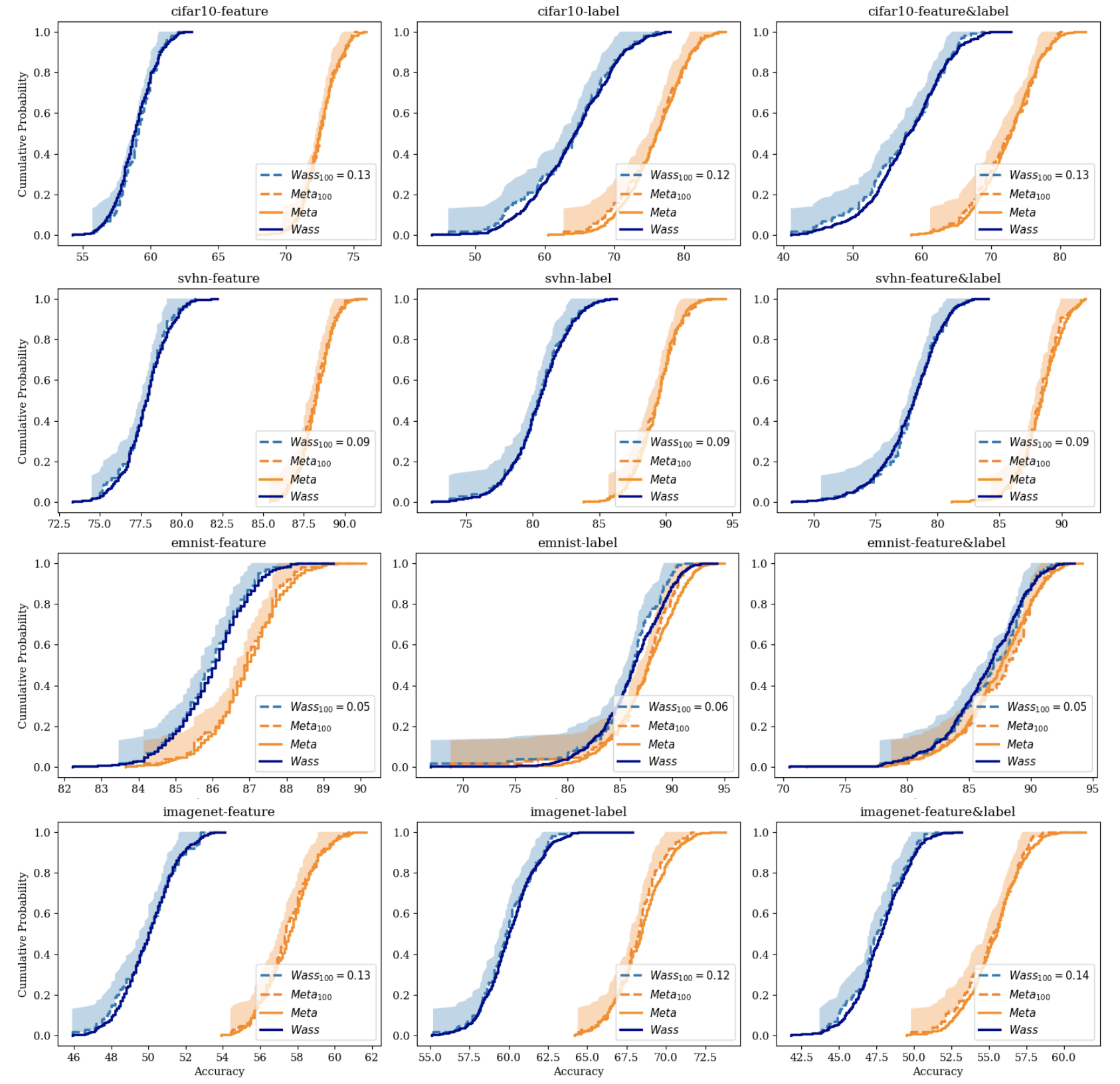
It should be noted that all bounds are asymptotically minimax optimal, meaning that an adversary can choose a distribution to perform exactly as bad as the bounds, at least in the asymptotic regime where both and tend to infinity.