Revisiting Differential Verification:
Equivalence Verification with Confidence

Abstract

When validated NN are pruned (and retrained) before deployment, it is desirable to prove that the new NN behaves equivalently to the (original) reference NN.To this end, our paper revisits the idea of differential verification which performs reasoning on differences between NN:On the one hand, our paper proposes a novel abstract domain for differential verification admitting more efficient reasoning about equivalence.On the other hand, we investigate empirically and theoretically which equivalence properties are (not) efficiently solved using differential reasoning.Based on the gained insights, and following a recent line of work on confidence-based verification, we propose a novel equivalence property that is amenable to Differential Verification while providing guarantees for large parts of the input space instead of small-scale guarantees constructed w.r.t. predetermined input points.We implement our approach in a new tool called VeryDiff and perform an extensive evaluation on numerous old and new benchmark families, including new pruned NN for particle jet classification in the context of CERN’s LHC where we observe median speedups $>300\times$ over the State-of-the-Art verifier $\alpha,\beta$-CROWN.

1 Introduction

Specifying what an NN is supposed to do is a difficult problem, that is at most partially solved.One class of specifications that is comparatively easy to formalize are equivalence properties:Given an “old” reference NN $f_{1}$, we aim to prove that a “new” NN $f_{2}$ behaves in some way equivalently.For example $\varepsilon$ equivalence [25, 30] requires that the numerical outputs of $f_{1}$ and $f_{2}$ for the same input point differ by at most $\varepsilon$ or Top-1 equivalence [25] requires that the two NN’ classifications match.Known applications of equivalence verification are verification after retraining or pruning [41], student-teacher training [25, 36], analysis of sensitivity to NN-based preprocessing steps [29] and construction of quantized NN [27].Several publications [30, 31, 25, 36, 15, 41, 20] have proposed methods for the verification of equivalence properties (sometimescalling it “approximate conformance”).While it is known that equivalence verification w.r.t. the $\varepsilon$ equivalence (Definition 2) property is coNP-complete [36], the complexity-theoretic status of Top-1 equivalence verification (Definition 3) was to date unclear.

Contribution.

This work encompasses multiple theoretical and practical contributions to the field of equivalence verification:

• We prove that deciding if two $\mathrm{ReLU}{}$ NN are Top-1 equivalent is a coNP-complete decision problem, i.e. it is as hard as $\varepsilon$-equivalence verification [36] or the classic NN verification problem [23, 32].

• We propose Differential Zonotopes: An abstract domain that allows the usage of the differential verification methodology w.r.t. the Zonotope abstract domain by propagating a Zonotope bounding the difference between two NN in lock-step with a reachability analysis for the individual NN.

• We implement the proposed approach in a new tool and evaluate its efficiency.For $\varepsilon$ equivalence we achieve median speedups >10 for 8 of 9 comparisons (4.5 in the other case).

• For Top-1 equivalence we demonstrate empirically that Differential Zonotopes do not aid verification.We provide a theoretical intuition for this observation and demonstrate this is a fundamental limitation of Differential Verification in general – independently of the chosen abstract domain.

• Based on these insights, we propose a new confidence-based equivalence property for classification NN which is 1. verifiable on larger parts of the input space of NN; 2. amenable to differential verification. Furthermore, we propose a simpler and more precise linear approximation of the $\mathrm{softmax}$ function in comparison to prior work [2].In additional experiments, we demonstrate that our tool can certify 327% more benchmark queries than $\alpha,\beta$-CROWN for confidence-based equivalence.

Related Work.

Prior work on Zonotope-based NN verification [16, 35] verified non-relational properties w.r.t. a single NN.We extend this work by providing a methodology that allows reasoning about differences between NN.Equivalence properties, can in principle, be analyzed using classical NN verification techniques such as $\alpha,\beta$-CROWN [zhang22babattack, xu2020automatic, zhang2018efficient, zhang2022general, 33]for a single NN by building “product-networks” (similar to product-programs in classical program verification [8]), but early work on NN equivalence verification demonstrated that this approach is inefficient due to the accumulation of overapproximation errors in the two independent NN [30].While this view was recently challenged by [20], Section 7 conclusively demonstrates that tailored verification tools still outperform State-of-the-Art “classical” NN verification tools for NN with similar weight structures.Prior work suggested using Star-Sets for equivalence verification without analyzing weight differences and heavily relied on LP solving [36].Prior work on differential verification [30, 31] did not verify the equivalence of classifications and also fell short of using the Zonotope abstract domain.Section 7 compares to equivalence verifiers [31, 25, 36].In another line of work, QEBVerif [DBLP:conf/cav/ZhangSS23] proposes a sound and complete analysis technique tailored to quantized NN which is not directly applicable to other kinds of NN studied in our evaluation.Another line of research analyzes relational properties w.r.t. multiple runs of a single NN.All listed works do not verify equivalence.For example, Banerjee et al. [7] propose an abstract domain for relational properties, but assume that all executions happen on the same NN.This makes their approach incompatible with our benchmarks which require the analysis of multiple different NN.Another incomplete relational verifier [6] also assumes executions on a single NN and requires tailored relaxations not available for equivalence properties.Encoding relational properties via product NN has also been explored by Athavale et al. [2].We compare against Marabou (which they used) and we prove that our approximation of softmax, though simpler, is always more precise.

Overview.

Section 2 introduces the necessary background on NN verification via Zonotopes, equivalence verification and confidence based NN verification.Section 3 proves the coNP-completeness of Top-1 equivalence.Subsequently, we introduce Differential Zonotopes as an abstract domain for differential reasoning via Zonotopes (Section 4) and explain how Differential Zonotopes can be used to perform equivalence verification (Section 5).Section 6 explains why Top-1 equivalence does not benefit from differential reasoning in general and derives a new confidence-based equivalence property that may hold on large parts of the input space and can be verified more efficiently using differential verification.Finally, Section 7 provides an evaluation of our approach.

2 Background

We deal with the verification of piece-wise linear, feed-forward NN.A NN with input dimension $I\in\mathbb{N}$ and output dimension $O\in\mathbb{N}$ and $L\in\mathbb{N}$ layers can be summarized as a function $f:\mathbb{R}^{I}\to\mathbb{R}^{O}$ which maps input vectors $\mathbf{x}^{(0)}\in\mathbb{R}^{I}$ to output vectors $\mathbf{x}^{(L)}\in\mathbb{R}^{O}$.In more detail, each layer of the NN consists of an affine transformation $\tilde{\mathbf{x}}^{(i)}=W^{(i)}\mathbf{x}^{(i-1)}+b^{(i)}$ (for a matrix $W^{(i)}$ and a vector $b^{(i)}$) followed by the application of a non-linear function $\mathbf{x}^{(i)}=h^{(i)}\left(\tilde{\mathbf{x}}^{(i)}\right)$.Many feed-forward architectures can be compiled into this format [34].We focus on the case of NN with $\mathrm{ReLU}$ activations, i.e. $h^{(i)}\left(\tilde{\mathbf{x}}^{(i)}\right)=\mathrm{ReLU}\left(\tilde{\mathbf{x}}^{(i)}\right)=\max\left(0,\tilde{\mathbf{x}}^{(i)}\right)$ for all$1\leq i\leq L$.$f^{(i)}\left(\mathbf{x}\right)$ is the computation of the NN’s first $i$ layers.We uniformly denote vectors in bold ($\mathbf{v}$) and matrices in capital letters ($M$) and Affine Forms/Zonotopes are denoted as /$\mathcal{Z}$.

NN Verification.

A well-known primitive in the literature on NN verification are Zonotopes [16, 35]: An abstract domain that allows the efficient propagation of an interval box over the input space through (piece-wise) affine systems:

Definition 1 (Zonotope).

A Zonotope with input dimension $n$ and output dimension $m$ isa collection of $m$ Affine Forms of the structure

$$\mathbf{g}\mathbf{\epsilon}+c \left(\mathbf{\epsilon}\in\left[-1,1\right]^{n},\mathbf{g}\in\mathbb{R}^{n},c\in\mathbb{R}\right)$$

We denote a single Affine Form as a tuple $\left(\mathbf{g},c\right)$.Given an Affine Form $\text{\textctyogh}{}=\left(\mathbf{g},c\right)$ and a vector $\mathbf{v}\in\left[-1,1\right]^{d}$ ($d\leq n$) we denote by $\text{\textctyogh}{}\left(\mathbf{v}\right)$ the Affine Form (or value for $d=n$) where the first $d$ values of $\mathbf{\epsilon}$ are fixed to $\mathbf{v}$, i.e. to $\left(\mathbf{g}_{d+1:n},\mathbf{g}_{1:d}\mathbf{v}+c\right)$.For $\text{\textctyogh}{}=\left(\mathbf{g},c\right)$, we denote the set of points described by as $\langle\text{\textctyogh}{}\rangle=\left\{\text{\textctyogh}{}\left(\mathbf{\epsilon}\right)~{}\middle|~{}\mathbf{\epsilon}\in\left[-1,1\right]^{n}\right\}$.

Via $\text{\textctyogh}{}\left(\mathbf{v}\right)$ we denote the values reachable given the (input) vector $\mathbf{v}$.To improve clarity, some transformations applied to Zonotopes will be described for the 1-dimensional case, i.e. to a single Affine Form.Nonetheless, a major advantage of Zonotopes lies in their Matrix representation: $m$ Affine Forms are then a matrix $G\in\mathbb{R}^{n\times m}$ and a vector $\mathbf{c}\in\mathbb{R}^{m}$ (then denoted as $\mathcal{Z}{}=\left(G,\mathbf{c}\right)$).A component of $\mathbf{g}$/a column of $G$ is called a generator.Given a Zonotope $\mathcal{Z}{}$ we denote its $i$-th Affine Form (represented by $G$’s $i$-th row and $\mathbf{c}$’s $i$-th component) as $\mathcal{Z}{}_{i}$.Similar to the affine forms, we define$\langle\mathcal{Z}\rangle=\left\{\mathbf{x}\in\mathbb{R}^{m}\middle|\mathbf{\epsilon}\in\left[-1,1\right]^{n},\mathbf{x}_{i}=\mathcal{Z}_{i}\left(\mathbf{\epsilon}\right)\right\}$.Zonotopes are a good fit for analyzing (piece-wise) linear NN as they are closed under affine transformations [5]:

Proposition 1 (Affine Zonotope Transformation).

For some Zonotope $\mathcal{Z}=\left(G,\mathbf{c}\right)$ and an affine transformation $h\left(\mathbf{x}\right)=W\mathbf{x}+\mathbf{b}$,the Affine Form $\hat{\mathcal{Z}}=\left(WG,W\mathbf{c}+\mathbf{b}\right)$ exactly describes the affine transformation applied to the points $x\in\langle\mathcal{Z}\rangle$, i.e.for all $d\leq n$ and $\mathbf{v}\in\left[-1,1\right]^{d}$:$\left\{W\mathbf{x}+\mathbf{b}~{}\middle|~{}\mathbf{x}\in\langle\mathcal{Z}\left(\mathbf{v}\right)\rangle\right\}=\langle\hat{\mathcal{Z}}\left(\mathbf{v}\right)\rangle$

This proposition implies $\left\{W\mathbf{x}+\mathbf{b}~{}\middle|~{}\mathbf{x}\in\langle\mathcal{Z}{}\rangle\right\}=\langle\hat{\mathcal{Z}{}}\rangle$, but it is even strongeras it also guarantees a linear map from an input ($\mathbf{v}$) to all reachable outputs ($\langle\hat{\mathcal{Z}{}}\left(\mathbf{v}\right)\rangle$).Zonotopes also admit efficient computation of interval bounds for their outputs:

Proposition 2 (Zonotope Output Bounds).

Consider some Affine Form $\text{\textctyogh}{}=\left(\mathbf{g},c\right)$it holds for all $\mathbf{x}\in\left[-1,1\right]^{n}$ that:

$$\mathbf{g}\mathbf{x}+c\in\left[\underline{\text{\textctyogh}{}},\overline{\text{\textctyogh}{}}\right]\coloneqq\left[c-\sum_{i=0}^{n}\left|\mathbf{g}_{i}\right|,c+\sum_{i=0}^{n}\left|\mathbf{g}_{i}\right|\right]$$

Figure 1: $\mathrm{ReLU}$ approximation

Zonotopes cannot exactly represent the application of $\mathrm{ReLU}$, but we can approximate the effect by distinguishing three cases: 1. The upper-bound $\overline{\text{\textctyogh}{}}$ is negative and thus $\mathrm{ReLU}\left(x\right)=0$ for $x\in\langle\text{\textctyogh}{}\rangle$; 2. The lower-bound $\underline{\text{\textctyogh}{}}$ is positive and thus $\mathrm{ReLU}\left(x\right)=x$ for $x\in\langle\text{\textctyogh}{}\rangle$; 3. The $\mathrm{ReLU}{}$-node is instable and its output is thus piece-wise linear. The first and second case can be represented as an affine transformation and the third case requires an approximation (see Figure 1 for intuition):Interpolation between $\mathrm{ReLU}\left(x\right)=0$ and $\mathrm{ReLU}\left(x\right)=x$ (see the blue line in Figure 1 and $\lambda\mathbf{g}$ in Proposition 3) yields a representation, that we can turn into a sound overapproximation (meaning all possible output values of $\mathrm{ReLU}\left(x\right)$ are contained).This is achieved by adding a new generator that appropriately bounds the error of the interpolated function (see orange lines in Figure 1 and $\tfrac{1}{2}\lambda\underline{\text{\textctyogh}{}}$ in Proposition 3).This result is summarized as follows:

Proposition 3 ($\mathrm{ReLU}$ Zonotope Transformation [35]).

Consider some Affine Form $\text{\textctyogh}{}=\left(\mathbf{g},c\right)$.Define a new Affine Form $\hat{\text{\textctyogh}{}}=\left(\hat{\mathbf{g}},\hat{c}\right)$ such that:

$$\hat{\mathbf{g}} =0\in\mathbb{R}^{n} \hat{c} =0 \text{if }\overline{z}<0$$

$$\hat{\mathbf{g}} =\mathbf{g}\in\mathbb{R}^{n} \hat{c} =c \text{if }\underline{z}>0$$

$$\hat{\mathbf{g}} =\left(\begin{array}[]{c}\lambda\mathbf{g}\\ \tfrac{1}{2}\lambda\underline{\text{\textctyogh}{}}\end{array}\right)\in\mathbb{R}^{n+1} \hat{c} =c-\tfrac{1}{2}\lambda\underline{\text{\textctyogh}{}}$$ else

for $\lambda=\frac{\overline{\text{\textctyogh}{}}}{\left(\overline{\text{\textctyogh}{}}-\underline{\text{\textctyogh}{}}\right)}$.Then $\hat{\text{\textctyogh}{}}$ guarantees for all $d\leq n$ and $\mathbf{v}\in\left[-1,1\right]^{d}$ that:

$$\left\{\mathrm{ReLU}\left(x\right)\middle|x\in\langle\text{\textctyogh}{}\left(\mathbf{v}\right)\rangle\right\}\subseteq\langle\hat{\text{\textctyogh}{}}\left(\mathbf{v}\right)\rangle$$

NN verification via Zonotopes typically proceeds as follows:An input set described as Zonotope is propagated through the NN using the transformers from Propositions 1 and 3.This yields an overapproximation of the NN’s behavior.Depending on the verification property, one can either check the property by computing the Zonotope’s bounds (Proposition 2) or by solving a linear program.If a property cannot be established, the problem is refined by either splitting the input space, w.r.t. its dimensions (input-splitting, e.g. [35]) or w.r.t. a particular neuron to eliminate the $\mathrm{ReLU}{}$’s nonlinearity (neuron-splitting, e.g. [5]).

Equivalence Verification.

To show that two NN $f_{1},f_{2}$ behave equivalently, we can, for example, verify that the NN’ outputs are equal up to some $\varepsilon$:

Definition 2 ($\varepsilon$ Equivalence [25, 30]).

Given two NN $f_{1},f_{2}:\mathbb{R}^{I}\to\mathbb{R}^{O}$ and an input set $X\subseteq\mathbb{R}^{I}$ we say $g_{1}$ and $g_{2}$ are $\varepsilon$ equivalent w.r.t. a $p$-norm iff for all $\mathbf{x}\in X$ it holds that $\left\lVert f_{1}\left(\mathbf{x}\right)-f_{2}\left(\mathbf{x}\right)\right\rVert_{p}<\varepsilon$

Deciding $\varepsilon$ equivalence is coNP-complete [36].Another line of work proposes verification of Top-1 equivalence which is important for classification NN [25]:

Definition 3 (Top-1 Equivalence [25]).

Given two NN $f_{1},f_{2}:\mathbb{R}^{I}\to\mathbb{R}^{O}$ and an input set $X\subseteq\mathbb{R}^{I}$, $f_{1}$ and $f_{2}$ are Top-1 equivalent iff for all $\mathbf{x}\in X$ we have $\mathrm{argmax}_{i}~{}f_{1,i}\left(\mathbf{x}\right)=\mathrm{argmax}_{i}~{}f_{2,i}\left(\mathbf{x}\right)$, i.e. for every $k\in\left[1,O\right],\mathbf{x}\in X$ it holds $f_{1,k}\left(\mathbf{x}\right)\geq f_{1,j}\left(\mathbf{x}\right)$ (for all $j\neq k$) implies that $f_{2,k}\left(\mathbf{x}\right)\geq f_{2,j}\left(\mathbf{x}\right)$ (for all $j\neq k$).

For $\varepsilon$ equivalence, prior work by Paulsen et al. [30, 31] introduced differential verification: For two NN of equal depth (i.e. $L_{1}=L_{2}$),equivalence can be verified more effectively by reasoning about weight differences.To this end, Paulsen et al. used symbolic intervals [38, 39] not only for bounding values of a single NN, but to bound the difference of values between two NN $f_{1},f_{2}$, i.e. at any layer $1\leq i\leq L$ we compute two linear symbolic bound functions $l^{(i)}_{\Delta}\left(\mathbf{x}\right),u^{(i)}_{\Delta}\left(\mathbf{x}\right)$ such that $l^{(i)}_{\Delta}\left(\mathbf{x}\right)\leq f_{1}^{(i)}\left(\mathbf{x}\right)-f_{2}^{(i)}\left(\mathbf{x}\right)\leq u^{(i)}_{\Delta}\left(\mathbf{x}\right)$.Differential bounds are computed by propagating symbolic intervals through two NN in lock-step.This enables the computation of bounds on the difference at every layer.

Confidence Based Verification

Many classification NN provide a confidence for their classification by using the Softmax function $\mathrm{softmax}_{i}\left(x\right)=\frac{e^{x_{i}}}{\sum_{i=1}^{n}x_{i}}$.A recent line of work [2] proposes to use the confidence values classically provided by classification NN as a starting point for verification.For example, Athavale et al. [2] propose a global, confidence-based robustness property which stipulates that inputs classified with high confidence must be robust to noise (i.e. we require the same classification for some bounded perturbation of the input).While this introduces reliance on the NN’s confidence, it enables global specifications verified on the full input space and this limitation can be addressed by an orthogonal direction of research that aims at training calibrated NN [18, 1], i.e. NN that correctly estimate the confidence of their predictions.

3 Complexity of Top-1 Verification

Prior work showed that the classic NN verification problemfor a single $\mathrm{ReLU}$-NN is an NP-complete problem [23, 32]. main-pratenddefaultcategory.texmain-pratenddefaultcategory.texSimilarly, the problem of finding a violation for $\varepsilon$ equivalence is NP-complete for $\mathrm{ReLU}$-NNas the single-NN verification problem can be reduced to this setting [36].We now show, that finding a violation of Top-1 equivalence (Top-1-Net-Equiv) is also NP-complete implying that proving absence of counterexamples is coNP-complete (see proof on LABEL:proof:nn_program_existence):[Top-1-Net-Equiv is coNP-complete][end,restate,text link=]Let $X\subseteq\mathbb{R}^{I}$ be some polytope over the input space of two $\mathrm{ReLU}{}$-NN $f_{1},f_{2}$.Deciding whether there exists $\mathbf{x}\in X$ and a $k\in\left[1,O\right]$ s.t. $\left(f_{1}\left(\mathbf{x}\right)\right)_{k}\geq\left(f_{1}\left(\mathbf{x}\right)\right)_{i}$ for all $i\in\left[1,O\right]$ but for some $j\in\left[1,O\right]$ it holds that $\left(f_{2}\left(\mathbf{x}\right)\right)_{k}<\left(f_{2}\left(\mathbf{x}\right)\right)_{j}$ is NP-complete.

Proof Sketch.

Our proof differs from the proof for $\varepsilon$ equivalence in the reduced problem which is the “classical” NN verification problem [23, 32] for $\varepsilon$ equivalence verification.To apply a similar proof technique to Top-1 equivalence, we require an NN verification instance with only strict inequality constraints in the input and output.Therefore, we first prove the NP-completeness of verifying strict inequality constraints (LABEL:def:strict_net_verify in LABEL:apx:proofs) by adapting prior proofs [23, 32].Then, we can reduce this problem to Top-1 equivalence verification.The reduction works by constructing an instance of Top-1-Net-Equiv that has a Top-1 violation iff the violating input also satisfies the constraints of the original NN verification problem.∎

See proof in appendix on page LABEL:proof:prAtEnd\pratendcountercurrent.main-pratenddefaultcategory.tex main-pratenddefaultcategory.tex

4 Equivalence Analysis via Zonotopes

Given two NN $f_{1},f_{2}:\mathbb{R}^{I}\to\mathbb{R}^{O}$ with $L$ layers each,we follow the basic principle of differential verification, i.e. we bound the difference $f_{1}^{(i)}-f_{2}^{(i)}$ at every layer $1\leq i\leq L$.For our presentation, we assume that all layers of the NN have the same width, i.e. the same number of nodes.In practice, this limitation can be lifted by enriching the thinner layer with zero rows [41].Our approach to differential verification is summarized in Algorithm 1:First and foremost, we perform a classic reachability analysis via Zonotopes for the two NN $f_{1},f_{2}$.To this end, we propagate a given input Zonotope $\mathcal{Z}{}_{\text{in}}$ through both NN resulting in output Zonotopes $\mathcal{Z}{}^{\prime},\mathcal{Z}{}^{\prime\prime}$.This part of the analysis uses the well-known Zonotope transformers described in Propositions 1 and 3.The individual reachability analysis is complemented with the computation of the Differential Zonotope $\mathcal{Z}{}^{\Delta}$ which is initialized with $0$ (meaning the NN’s inputs are initially equal) and computed in lock-step to the computation of $\mathcal{Z}{}^{\prime}$ and $\mathcal{Z}{}^{\prime\prime}$:At every layer, we overapproximate the maximal deviation between the two NN.Using the transformers described in the remainder of this Section, we can prove that the Differential Zonotope always overapproximates the difference between the two NN (see proof on LABEL:proof:verydiff_verysound):[Soundness][end,restate,text link=]Let $f_{1},f_{2}$ be two feed-forward ReLU-NN, $\mathcal{Z}{}_{\text{in}}$ some Zonotope mapping $n$ generators to $I$ dimensions and $\mathcal{Z}{}^{\prime},\mathcal{Z}{}^{\prime\prime},\mathcal{Z}{}^{\Delta}$ the output of $\textsc{Reach}_{\Delta}\left(f_{1},f_{2},\mathcal{Z}{}_{\text{in}}\right)$.The following statements hold for all $\mathbf{v}\in\left[-1,1\right]^{n}$:

1. $f_{1}\left(\mathcal{Z}{}_{\text{in}}\left(\mathbf{v}\right)\right)\in\langle\mathcal{Z}{}^{\prime}\left(\mathbf{v}\right)\rangle$ and $f_{2}\left(\mathcal{Z}{}_{\text{in}}\left(\mathbf{v}\right)\right)\in\langle\mathcal{Z}{}^{\prime\prime}\left(\mathbf{v}\right)\rangle$

2. $\big{(}~{}f_{1}\left(\mathcal{Z}{}_{\text{in}}\left(\mathbf{v}\right)\right)-f_{2}\left(\mathcal{Z}{}_{\text{in}}\left(\mathbf{v}\right)\right)~{}\big{)}\in\langle\mathcal{Z}{}^{\Delta}\left(\mathbf{v}\right)\rangle$

See proof in appendix on page LABEL:proof:prAtEnd\pratendcountercurrent.main-pratenddefaultcategory.tex[Bound on output difference][all end]Let $f_{1},f_{2}$ be two feed-forward ReLU-NN, $\mathcal{Z}{}_{\text{in}}$ some Zonotope with input dimension $n$ and output dimension $I$ and $\mathcal{Z}{}^{\prime},\mathcal{Z}{}^{\prime\prime},\mathcal{Z}{}^{\Delta}$ the output of $\textsc{Reach}_{\Delta}\left(f_{1},f_{2},\mathcal{Z}{}_{\text{in}}\right)$.For all $\mathbf{v}\in\left[-1,1\right]^{n}$:

$$\big{(}f_{1}\left(\mathcal{Z}{}_{\text{in}}\left(\mathbf{v}\right)\right),f_{2}\left(\mathcal{Z}{}_{\text{in}}\left(\mathbf{v}\right)\right)\big{)}\in\langle\left(\mathcal{Z}{}^{\prime}\left(\mathbf{v}\right),\mathcal{Z}{}^{\prime\prime}\left(\mathbf{v}\right),\mathcal{Z}{}^{\Delta}\left(\mathbf{v}\right)\right)\rangle.$$

See proof in appendix on page LABEL:proof:prAtEnd\pratendcountercurrent.main-pratenddefaultcategory.tex

Algorithm 1 Verification with Differential Zonotopes

NN $g_{1},g_{2}:\mathbb{R}^{I}\to\mathbb{R}^{O}$with $L$layers, Input-Zonotope $Z_{\text{in}}=\left(G_{\text{in}},b_{\text{in}}\right)$Reachable Zonotopes $\mathcal{Z}{}^{\prime},\mathcal{Z}{}^{\prime\prime},\mathcal{Z}{}^{\Delta}$$\textsc{Reach}_{\Delta}$$g_{1},g_{2},Z_{\text{in}}$

$\mathcal{Z}{}^{\prime}\leftarrow Z_{\text{in}}$

$\mathcal{Z}{}^{\prime\prime}\leftarrow\text{copy}\left(Z_{\text{in}}\right)$

$\mathcal{Z}{}^{\Delta}\leftarrow\left(0,0\right)\in\mathbb{R}^{I\times I}\times\mathbb{R}^{I}$$\triangleright$ Initialize Differential Zonotope with 0$l\in\left[1,L\right]$layer $l$ is affine

$\mathcal{Z}{}^{\Delta}\leftarrow\textsc{Affine}_{\Delta}\left(\mathcal{Z}{}^{\Delta},\mathcal{Z}{}^{\prime},\mathcal{Z}{}^{\prime\prime},W^{(l)}_{1/2},\mathbf{b}^{(l)}_{1/2}\right)$

$\triangleright$ See Section 4

$\mathcal{Z}{}^{\prime}\leftarrow\textsc{Affine}\left(\mathcal{Z}{}^{\prime},W^{(l)}_{1},\mathbf{b}^{(l)}_{1}\right)$

$\triangleright$ See Transformation in Proposition 1

$\mathcal{Z}{}^{\prime\prime}\leftarrow\textsc{Affine}\left(\mathcal{Z}{}^{\prime\prime},W^{(l)}_{2},\mathbf{b}^{(l)}_{2}\right)$

$\triangleright$ See Transformation in Proposition 1$\triangleright$ Transformation for $\mathrm{ReLU}$ Layer

$\hat{\mathcal{Z}{}}^{\prime},\hat{\mathcal{Z}{}}^{\prime\prime}\leftarrow\textsc{ReLU}\left(\mathcal{Z}{}^{\prime}\right),\textsc{ReLU}\left(\mathcal{Z}{}^{\prime\prime}\right)$

$\triangleright$ See Transformation in Proposition 3

$\mathcal{Z}{}^{\Delta}\leftarrow\textsc{ReLU}_{\Delta}\left(\mathcal{Z}{}^{\Delta},\mathcal{Z}{}^{\prime},\mathcal{Z}{}^{\prime\prime},\hat{\mathcal{Z}{}}^{\prime},\hat{\mathcal{Z}{}}^{\prime\prime}\right)$

$\triangleright$ See Section 4

$\mathcal{Z}{}^{\prime},\mathcal{Z}{}^{\prime\prime}\leftarrow\hat{\mathcal{Z}{}}^{\prime},\hat{\mathcal{Z}{}}^{\prime\prime}$$\mathcal{Z}{}^{\prime},\mathcal{Z}{}^{\prime\prime},\mathcal{Z}{}^{\Delta}$

For the descriptions of transformations, we again focus on a single Affine Form.In this section, we denote the representation of an Affine Form as $\text{\textctyogh}{}=\left(\mathbf{e},\mathbf{a},c\right)$ where $\mathbf{e}$ are the $n$ original (exact) generators present in an Affine Form of $\left(\mathcal{Z}{}_{\text{in}}\right)_{i}$ and $\mathbf{a}$ are the $p$ (approximate) generators added via $\mathrm{ReLU}$ transformations.For Differential Affine Forms we split the approximate generators into $\mathbf{a}^{\prime\Delta},\mathbf{a}^{\prime\prime\Delta}$ and $\mathbf{a}^{\Delta}$,distinguishing their origin ($\text{\textctyogh}{}{}^{\prime}$,$\text{\textctyogh}{}^{\prime\prime}$ or generators added to $\text{\textctyogh}{}^{\Delta}$ directly).This yields the Affine Form $\text{\textctyogh}{}^{\Delta}=\left(\mathbf{e}^{\Delta},\mathbf{a}^{\prime\Delta},\mathbf{a}^{\prime\prime\Delta},\mathbf{a}^{\Delta},c^{\Delta}\right)$.We assume that the corresponding vectors have equal dimensions (i.e. $\mathbf{e}^{\prime}$,$\mathbf{e}^{\prime\prime}$ and $\mathbf{e}^{\Delta}$ all have dimension $n_{1}$; $\mathbf{a}^{\prime}$ and $\mathbf{a}^{\prime\Delta}$ have dimension $n_{2}$ and $\mathbf{a}^{\prime\prime}$ as well as $\mathbf{a}^{\prime\prime\Delta}$ have dimension $n_{3}$).The points described by two Affine Forms and a Differential Affine Form are then described via common generator values$\mathbf{\epsilon_{1}},\mathbf{\epsilon_{2}},\mathbf{\epsilon_{3}},\mathbf{\epsilon_{4}}$ across all three Affine Forms.This definition naturally generalizes to the multidimensional (Zonotope) case by fixing all $\mathbf{\epsilon}$ values across dimensions and Zonotopes.We also denote the points contained in a tuple $\left(\text{\textctyogh}{}^{\prime},\text{\textctyogh}{}^{\prime\prime},\text{\textctyogh}{}^{\Delta}\right)$ using $\langle\cdot\rangle$:

Definition 4 (Points Contained by Differential Affine Form).

Given two Affine Forms $\text{\textctyogh}{}^{\prime}=(\mathbf{e}^{\prime},\mathbf{a}^{\prime},c^{\prime}),\text{\textctyogh}{}^{\prime\prime}=\left(\mathbf{e}^{\prime\prime},\mathbf{a}^{\prime\prime},c^{\prime\prime}\right)$ and a Differential Affine Form $\text{\textctyogh}{}^{\Delta}=\left(\mathbf{e}^{\Delta},\mathbf{a}^{\prime\Delta},\mathbf{a}^{\prime\prime\Delta},\mathbf{a}^{\Delta},c^{\Delta}\right)$ with resp. a matching number of columns, we define the set of points described by $(\text{\textctyogh}{}^{\prime},\text{\textctyogh}{}^{\prime\prime},\text{\textctyogh}{}^{\Delta})$ where $n_{1},n_{2},n_{3},n_{4}$ are resp. the number of columns in $\mathbf{e}^{\Delta},\mathbf{a}^{\prime\Delta},\mathbf{a}^{\prime\prime\Delta},\mathbf{a}^{\Delta}$ and $\overline{n}=n_{1}+n_{2}+n_{3}+n_{4}$:

$$\langle(\text{\textctyogh}{}^{\prime},\text{\textctyogh}{}^{\prime\prime},\text{\textctyogh}{}^{\Delta})\rangle =$$

$$\Big{\{}\left(x,y\right)~{}\Big{|} ~{}\exists~{}\mathbf{\epsilon_{1}}\in\left[-1,1\right]^{n_{1}},~{}\mathbf{\epsilon_{2}}\in\left[-1,1\right]^{n_{2}},~{}\mathbf{\epsilon_{3}}\in\left[-1,1\right]^{n_{3}},~{}\mathbf{\epsilon_{4}}\in\left[-1,1\right]^{n_{4}}~{}$$

$$x=\mathbf{e}^{\prime}\mathbf{\epsilon_{1}}+\mathbf{a}^{\prime}\mathbf{\epsilon_{2}}+c^{\prime}~{}\land~{}$$

$$y=\mathbf{e}^{\prime\prime}\mathbf{\epsilon_{1}}+\mathbf{a}^{\prime\prime}\mathbf{\epsilon_{3}}+c^{\prime\prime}~{}\land$$

$$(x-y)=\mathbf{e}^{\prime}\mathbf{\epsilon_{1}}+\mathbf{a}^{\prime\Delta}\mathbf{\epsilon_{2}}+\mathbf{a}^{\prime\prime\Delta}\mathbf{\epsilon_{3}}+\mathbf{a}^{\Delta}\mathbf{\epsilon_{4}}+c^{\Delta}\Big{\}}$$

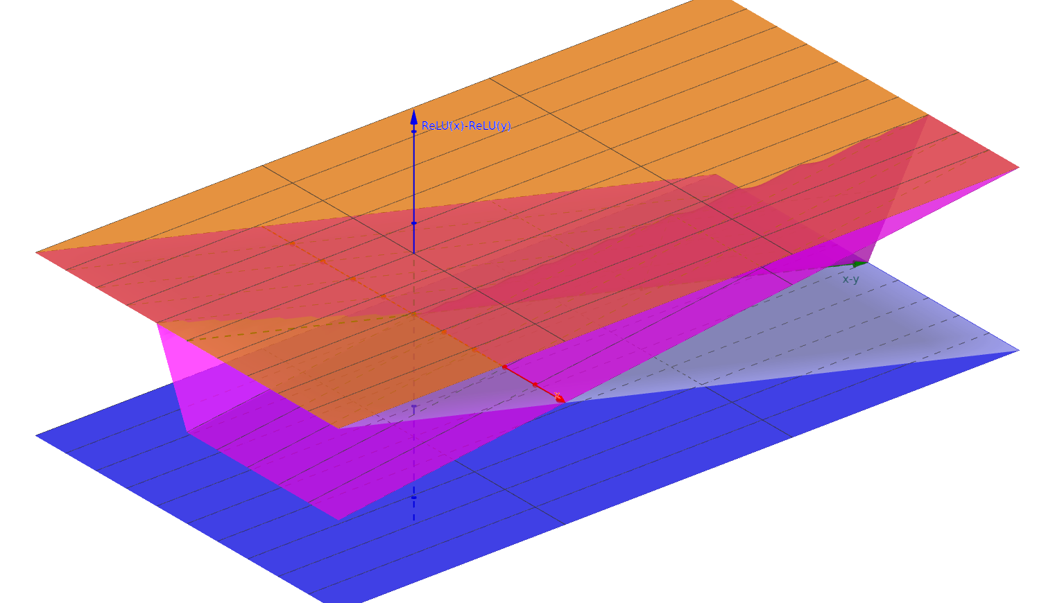
(a) Bounds on difference of two instable neurons.

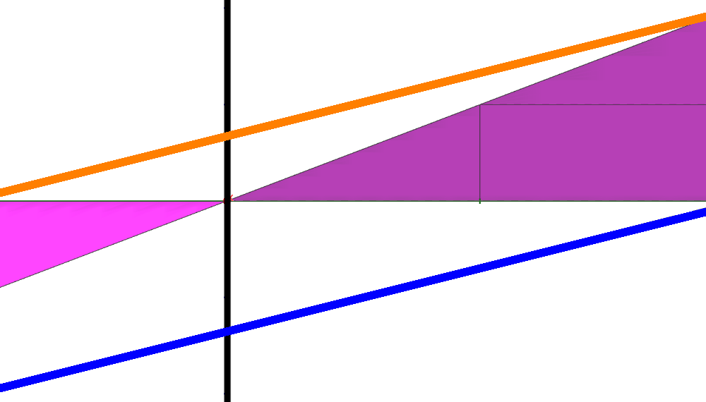
(b) Projection of Figure 3(a) w.r.t. neuron difference.

Figure 3: Visualization for the construction of a new Affine Form via $\textsc{ReLU}_{\Delta}$

Omitting the computation of $\mathcal{Z}{}^{\Delta}$, $\textsc{Reach}_{\Delta}$ corresponds to computing reachable outputs of $f_{1},f_{2}$ w.r.t. a common input Zonotope $\mathcal{Z}{}_{\text{in}}$.This algorithm implicitly computes the naive Differential Affine Form $\text{\textctyogh}{}^{\prime}-\text{\textctyogh}{}^{\prime\prime}$, i.e. the affine form $\text{\textctyogh}{}^{\Delta}=\left(\mathbf{e}^{\prime}-\mathbf{e}^{\prime\prime},\mathbf{a}^{\prime},-\mathbf{a}^{\prime\prime},0,c^{\prime}-c^{\prime\prime}\right)$.

Affine Transformations.

For affine transformations, we construct a transformation based on the insights from Differential Symbolic Bounds [30] that exactly two quantities determine the output difference:First, the difference accumulated so far (represented by the current Differential Affine Form $\text{\textctyogh}{}_{\Delta}$ and scaled by the layer’s affine transformation); second, the difference between the affine transformations in the current layer.Given two affine transformations $w^{(l)}_{1}x+b^{(l)}_{1}$ and $w^{(l)}_{2}x+b^{(l)}_{2}$ and Affine Forms $\text{\textctyogh}{}^{\prime}=\left(\mathbf{e}^{\prime},\mathbf{a}^{\prime},c^{\prime}\right),\text{\textctyogh}{}^{\prime\prime}=\left(\mathbf{e}^{\prime\prime},\mathbf{a}^{\prime\prime},c^{\prime\prime}\right),\text{\textctyogh}{}^{\Delta}=\left(\mathbf{e}^{\Delta},\mathbf{a}^{\prime\Delta},\mathbf{a}^{\prime\prime\Delta},\mathbf{a}^{\Delta},c^{\Delta}\right)$ wepropose $\textsc{Affine}_{\Delta}$ which returns a new Affine Form $\hat{\text{\textctyogh}{}}^{\Delta}=\left(\hat{\mathbf{e}}^{\Delta},\hat{\mathbf{a}}^{\prime\Delta},\hat{\mathbf{a}}^{\prime\prime\Delta},\hat{\mathbf{a}}^{\Delta},\hat{c}^{\Delta}\right)$ with:

$$\begin{aligned} \hat{\mathbf{e}}^{\Delta}&=w^{(l)}_{1}\mathbf{e}^{\Delta}+\left(w^{(l)}_{1}-w^{(l)}_{2}\right)\mathbf{e}^{\prime\prime}&\hat{\mathbf{a}}^{\prime\Delta}&=w^{(l)}_{1}\mathbf{a}^{\prime\Delta}\\ \hat{\mathbf{a}}^{\prime\prime\Delta}&=w^{(l)}_{1}\mathbf{a}^{\prime\prime\Delta}+\left(w^{(l)}_{1}-w^{(l)}_{2}\right)\mathbf{a}^{\prime\prime}&\hat{\mathbf{a}}^{\Delta}&=w^{(l)}_{1}\mathbf{a}^{\Delta}\\ \hbox to0.0pt{$\hat{c}^{\Delta}=w^{(l)}_{1}c^{\Delta}+\left(w^{(l)}_{1}-w^{(l)}_{2}\right)c^{\prime\prime}+\left(b^{(l)}_{1}-b^{(l)}_{2}\right)$\hss}\end{aligned}$$ (1)

We scale prior differences by $w^{(l)}_{1}$ and add the new difference $(w^{(l)}_{1}-w^{(l)}_{2})$ to $\hat{\mathbf{e}}^{\Delta}$, $\hat{\mathbf{a}}^{\prime\prime}$ (scaled by the reachable values of $f_{2}$, i.e. by $\text{\textctyogh}{}^{\prime\prime}$) and $\hat{c}^{\Delta}$ (and resp. $(b^{(l)}_{1}-b^{(l)}_{2})$).The transformation is sound (proof on LABEL:proof:diff_zono:zono_affine generalizes to Zonotopes):[Soundness of $\textsc{Affine}_{\Delta}$][end,restate,text link=]For affine transformations $\alpha_{1}\left(x\right)=w^{(l)}_{1}x+b^{(l)}_{1}$ and $\alpha_{2}\left(x\right)=w^{(l)}_{2}x+b^{(l)}_{2}$ and Affine Forms$\text{\textctyogh}{}^{\prime}=\left(\mathbf{e},\mathbf{a}^{\prime},c^{\prime}\right),\text{\textctyogh}{}^{\prime\prime}=\left(\mathbf{e}^{\prime\prime},\mathbf{a}^{\prime\prime},\mathbf{c}^{\prime\prime}\right),\text{\textctyogh}{}^{\Delta}=\left(\mathbf{e}^{\Delta},\mathbf{a}^{\Delta},\mathbf{a}^{\Delta},\mathbf{a}^{\Delta},c^{\Delta}\right)$ the transformation $\text{Affine}_{\Delta}$ is sound, i.e. if $\hat{\text{\textctyogh}{}}^{\Delta}$ is the result of $\textsc{Affine}_{\Delta}$, then for all $d\leq n$ and $\mathbf{v}\in\left[-1,1\right]^{d}$with $(x,y)\in\langle(\text{\textctyogh}{}^{\prime}\left(\mathbf{v}\right),\text{\textctyogh}{}^{\prime\prime}\left(\mathbf{v}\right),\text{\textctyogh}{}^{\Delta}\left(\mathbf{v}\right))\rangle$and $\hat{\text{\textctyogh}{}}^{\prime},\hat{\text{\textctyogh}{}}^{\prime\prime}$ the outputs of Affine (Proposition 1) we get:

$$\left(\alpha_{1}\left(x\right),\alpha_{2}\left(y\right)\right)\in\langle(\tilde{z}_{1}\left(v\right),\tilde{z}_{2}\left(v\right),\tilde{z}_{\Delta}\left(v\right))\rangle$$

See proof in appendix on page LABEL:proof:prAtEnd\pratendcountercurrent.main-pratenddefaultcategory.tex

$\mathrm{ReLU}$ Transformations.

Since $\mathrm{ReLU}$ is piece-wise linear, we cannot hope to construct an exact transformation for this case.However, by carefully distinguishing the possible cases (e.g. both nodes are solely negative, one is negative one is instable, etc.) we provide linear representations for 6 out of the 9 cases (both nodes stable or a negative and an instable node) while overapproximating the other three.Given $\text{\textctyogh}{}^{\prime}=\left(\mathbf{e}^{\prime},\mathbf{a}^{\prime},c^{\prime}\right),\text{\textctyogh}{}^{\prime\prime}=\left(\mathbf{e}^{\prime\prime},\mathbf{a}^{\prime\prime},c^{\prime\prime}\right)$ and a Differential Affine Form $\text{\textctyogh}{}^{\Delta}=\left(\mathbf{e}^{\Delta},\mathbf{a}^{\prime\Delta},\mathbf{a}^{\prime\prime\Delta},\mathbf{a}^{\Delta},c^{\Delta}\right)$as well as $\hat{\text{\textctyogh}{}}^{\prime},\hat{\text{\textctyogh}{}}^{\prime\prime}$ (the result of applying $\mathrm{ReLU}{}$ in the individual NN), we compute the result of the $\mathrm{ReLU}{}_{\Delta}$ transformation, using the case distinctions from Table 1.The transformation is sound (see LABEL:proof:diff_zono:zono_relu):[Soundness of $\mathrm{ReLU}{}_{\Delta}$][end,restate,text link=]Consider Affine Form $\text{\textctyogh}{}^{\prime}=\left(\mathbf{e},\mathbf{a}^{\prime},c^{\prime}\right),\text{\textctyogh}{}^{\prime\prime}=\left(\mathbf{e}^{\prime\prime},\mathbf{a}^{\prime\prime},\mathbf{c}^{\prime\prime}\right)$ and a Differential Affine Form $\text{\textctyogh}{}^{\Delta}=\left(\mathbf{e}^{\Delta},\mathbf{a}^{\prime\Delta},\mathbf{a}^{\prime\prime\Delta},\mathbf{a}^{\Delta},c^{\Delta}\right)$.Let $\hat{\text{\textctyogh}{}}^{\prime}$/$\hat{\text{\textctyogh}{}}^{\prime\prime}$ be the result of the ReLU transformation on $\text{\textctyogh}{}^{\prime}$/$\text{\textctyogh}{}^{\prime\prime}$ (see Proposition 3).Define $\hat{\text{\textctyogh}{}}^{\Delta}=\left(\hat{\mathbf{e}}^{\Delta},\hat{\mathbf{a}}^{\Delta},\hat{\mathbf{a}}^{\Delta},\hat{\mathbf{a}}^{\Delta},c^{\Delta}\right)$ such that it matches the case distinctions in Table 1.Then $\hat{\text{\textctyogh}{}}^{\Delta}$ overapproximates the behavior of $\mathrm{ReLU}{}$, i.e. for all $d\leq n$ and $\mathbf{v}\in\left[-1,1\right]^{d}$ with $(x,y)\in\langle(\text{\textctyogh}{}^{\prime}\left(\mathbf{v}\right),\text{\textctyogh}{}^{\prime\prime}\left(\mathbf{v}\right),\text{\textctyogh}{}^{\Delta}\left(\mathbf{v}\right))\rangle$ we get that:

$$\left(\mathrm{ReLU}\left(x\right),\mathrm{ReLU}\left(y\right)\right)\in\langle(\hat{\text{\textctyogh}{}}^{\prime}\left(\mathbf{v}\right),\hat{\text{\textctyogh}{}}^{\prime\prime}\left(\mathbf{v}\right),\hat{\text{\textctyogh}{}}^{\Delta}\left(\mathbf{v}\right))\rangle$$

See proof in appendix on page LABEL:proof:prAtEnd\pratendcountercurrent.main-pratenddefaultcategory.texUnfortunately, reasoning about the difference of two $\mathrm{ReLU}$s is not particularly intuitive.The first 6 cases in Table 1 follow from substituting Node 1 and Node 2 values.In the other cases (Positive + Instable and All Instable), the difference is not linear in the input or output Zonotopes.Thus, we append an additional generator to the Differential Zonotope, i.e. to $\mathbf{a}^{\Delta}$.The approximation for the case of two instable neurons is plotted in Figure 3:The bounding planes ensure that $0$ is always reachable and that the prior difference is within the bound.

Table 1: Case Distinction for the construction of a new Affine Form $\textsc{ReLU}_{\Delta}\left(\text{\textctyogh}{}^{\Delta},\text{\textctyogh}{}^{\prime},\text{\textctyogh}{}^{\prime\prime},\hat{\text{\textctyogh}{}}^{\prime},\hat{\text{\textctyogh}{}}^{\prime\prime}\right)=\hat{\text{\textctyogh}{}}^{\Delta}=\left(\hat{\mathbf{e}}^{\Delta},\hat{\mathbf{a}}^{\prime\Delta},\hat{\mathbf{a}}^{\prime\prime\Delta},\hat{\mathbf{a}}^{\Delta},\hat{c}^{\Delta}\right)$. Additions of vectors with different lengths signify addition for the components in the common-length prefix. We distinguish the nodes’ different phases by positive ($+$), negative (–), and instable ($\sim$). The variables $\lambda$, $\mu$ and $\nu$ are initialized as follows:$\lambda^{\prime}=\frac{-\underline{\text{\textctyogh}{}^{\prime}}}{\overline{\text{\textctyogh}{}^{\prime}}-\underline{\text{\textctyogh}{}^{\prime}}}$,$\mu^{\prime}=0.5*\lambda^{\prime}\overline{\text{\textctyogh}{}^{\prime}}$ (accordingly for $\lambda^{\prime\prime},\mu^{\prime\prime}$) and$\lambda^{\Delta}=\mathrm{clamp}\left(\frac{\overline{\text{\textctyogh}{}^{\Delta}}}{\overline{\text{\textctyogh}{}^{\Delta}}-\underline{\text{\textctyogh}{}^{\Delta}}},0,1\right)$,$\mu^{\Delta}=0.5*\max\left(-\underline{\text{\textctyogh}{}^{\Delta}},\overline{\text{\textctyogh}{}^{\Delta}}\right)$, $\nu^{\Delta}=\lambda^{\Delta}*\max\left(0,-\underline{\text{\textctyogh}{}^{\Delta}}\right)$

Neurons		New Affine Form $\hat{\text{\textctyogh}{}}^{\Delta}$
$f_{1}$	$f_{2}$	$\hat{\mathbf{e}}$	$\hat{\mathbf{a}}^{\prime\Delta}$	$\hat{\mathbf{a}}^{\prime\prime\Delta}$	$\hat{\mathbf{a}}^{\Delta}$	$\hat{c}$
Both nodes stable
–	–	$0$	$0$	$0$	$0$	$0$
–	+	$-\mathbf{e}^{\prime\prime}$	$0$	$-\mathbf{a}^{\prime\prime}$	$0$	$-c^{\prime\prime}$
+	–	$\mathbf{e}^{\prime}$	$\mathbf{a}^{\prime}$	$0$	$0$	$c^{\prime}$
+	+	$\mathbf{e}^{\Delta}$	$\mathbf{a}^{\prime\Delta}$	$\mathbf{a}^{\prime\prime\Delta}$	$\mathbf{a}^{\Delta}$	$c^{\Delta}$
Negative + Instable
$\sim$	–	$\hat{\mathbf{e}}^{\prime}$	$\hat{\mathbf{a}}^{\prime}$	$0$	$0$	$\hat{c}^{\prime}$
–	$\sim$	$-\hat{\mathbf{e}}^{\prime\prime}$	$0$	$-\hat{\mathbf{a}}^{\prime\prime}$	$0$	$-\hat{c}^{\prime\prime}$
Positive + Instable
$\sim$	+	$\mathbf{e}^{\Delta}-\lambda^{\prime}\mathbf{e}^{\prime}$	$\mathbf{a}^{\prime\Delta}-\lambda^{\prime}\mathbf{a}^{\prime}$	$\mathbf{a}^{\prime\prime\Delta}$	$((\mathbf{a}^{\Delta})^{T}\mid\mu^{\prime})^{T}$	$c^{\Delta}-\lambda^{\prime}c^{\prime}+\mu^{\prime}$
+	$\sim$	$\mathbf{e}^{\Delta}+\lambda^{\prime\prime}\mathbf{e}^{\prime\prime}$	$\mathbf{a}^{\prime\Delta}$	$\mathbf{a}^{\prime\prime\Delta}+\lambda^{\prime\prime}\mathbf{a}^{\prime\prime}$	$((\mathbf{a}^{\Delta})^{T}\mid\mu^{\prime\prime})^{T}$	$c^{\Delta}+\lambda^{\prime\prime}c^{\prime\prime}-\mu^{\prime\prime}$
All Instable
$\sim$	$\sim$	$\lambda^{\Delta}\mathbf{e}^{\Delta}$	$\lambda^{\Delta}\mathbf{a}^{\prime\Delta}$	$\lambda^{\Delta}\mathbf{a}^{\prime\prime\Delta}$	$\left(\lambda^{\Delta}(\mathbf{a}^{\Delta})^{T}\mid\mu^{\Delta}\right)^{T}$	$\lambda^{\Delta}c^{\Delta}+\nu^{\Delta}-\mu^{\Delta}$

5 Verification of Equivalence Properties

To verify equivalence with $\textsc{Reach}_{\Delta}$, we proceed as follows:We propagate a Zonotope $\mathcal{Z}{}_{\text{in}}$ through the two NN $f_{1},f_{2}$ as explained above.Subsequently, we check a condition on the outputs $\left(\mathcal{Z}{}^{\prime},\mathcal{Z}{}^{\prime\prime},\mathcal{Z}{}^{\Delta}\right)$ that implies the desired equivalence property.If this check fails, we refine the Zonotope by splitting the input space.For the naive case, we compute $\mathcal{Z}{}^{\Delta}$ as explained in Section 4.

$\varepsilon$ equivalence.

Checking $\varepsilon$ equivalence w.r.t. $\mathcal{Z}{}^{\Delta}$ works similarly to the approach for symbolic interval-based differential verification [30, 31]:We compute $\mathcal{Z}{}^{\Delta}$’s interval bounds and check for an absolute bound $>\varepsilon$.If all bounds are smaller, we have proven $\varepsilon$ equivalence for $\langle\mathcal{Z}{}_{\text{in}}\rangle$ (see also Section 5 in LABEL:apx:proofs).[Soundness of $\varepsilon$ equivalence check][all end]Let $\mathcal{Z}{}^{\prime},\mathcal{Z}{}^{\prime\prime},\mathcal{Z}{}^{\Delta}$ be $\textsc{Reach}_{\Delta}$’s result for two NN $f_{1},f_{2}$ and an input space described by $\mathcal{Z}{}_{\text{in}}$.If for all $1\leq i\leq O$ it holds that $\max\left(\left|\underline{\left(\mathcal{Z}{}^{\Delta}\right)_{i}}\right|,\left|\overline{\left(\mathcal{Z}{}^{\Delta}\right)_{i}}\right|\right)\leq\varepsilon$ then ${\forall\mathbf{x}\in\langle Z_{\text{in}}\rangle~{}\left(f_{1}\left(\mathbf{x}\right)-f_{2}\left(\mathbf{x}\right)\right)\leq\varepsilon}$. See proof in appendix on page LABEL:proof:prAtEnd\pratendcountercurrent.main-pratenddefaultcategory.tex

Top-1 Equivalence.

Since Top-1 equivalence considers the order of outputs, it cannot be read off from $\mathcal{Z}{}^{\Delta}$’s bounds directly.We frame the property as an LP optimization problem in Definition 5.The LP has an optimal solution $\leq 0$ if no $\mathbf{x}\in\langle\mathcal{Z}{}_{\text{in}}\rangle$ classified as $k$ in $f_{1}$ is classified as $j$ in $f_{2}$.Formally, the LP computes an upper bound for $\left(f_{2}\left(\mathbf{x}\right)\right)_{j}-\left(f_{2}\left(\mathbf{x}\right)\right)_{k}$ (maximized expression) under the condition that$\left(f_{1}\left(\mathbf{x}\right)\right)_{k}$ is the maximum of $f_{1}\left(\mathbf{x}\right)$ (first constraint) and under the additional condition that $\mathcal{Z}{}^{\Delta}$ bounds the difference between $f_{1}$ and $f_{2}$, resp. the difference between the reachable points in $\mathcal{Z}{}^{\prime}$ and $\mathcal{Z}{}^{\prime\prime}$ (second constraint; see Definition 5 in LABEL:apx:proofs).The first constraint ensures a gap $t$ between the largest and second largest output of $f_{1}$.In this section, we only consider $t=0$.

Definition 5 (Top-1 Violation LP).

Given $\mathcal{Z}{}^{\prime}=\left(G^{\prime},\mathbf{c}^{\prime}\right)=\left(E^{\prime},A^{\prime},\mathbf{c}^{\prime}\right),\mathcal{Z}{}^{\prime\prime}=\left(E^{\prime\prime},A^{\prime\prime},\mathbf{c}^{\prime\prime}\right),\mathcal{Z}{}^{\Delta}=\left(G^{\Delta},\mathbf{c}^{\Delta}\right)$, a constant $t\geq 0$ and $k,j\in\left[1,O\right]$ with $k\neq j$ the Top-1 Violation LP is defined below.$E^{\prime}$ and $E^{\prime\prime}$ have $n_{1}$ columns, $A^{\prime}$ has $n_{2}$ columns, $A^{\prime\prime}$ has $n_{3}$ columns and $A^{\Delta}$ has $n_{4}$ columns. $\mathbf{x}$ contains generators for these matrices in order and has dimension $\bar{n}=n_{1}+n_{2}+n_{3}+n_{4}$.

$$\max_{\mathbf{x}\in\left[-1,1\right]^{\overline{n}}} \left(E^{\prime\prime}\mathbf{x}_{1:n_{1}}+A^{\prime\prime}\mathbf{x}_{(n_{1}+n_{2}+1):(n_{1}+n_{2}+n_{3})}+\mathbf{c}\right)_{j}$$

$$-\left(E^{\prime\prime}\mathbf{x}_{1:n_{1}}+A^{\prime\prime}\mathbf{x}_{(n_{1}+n_{2}+1):(n_{1}+n_{2}+n_{3})}+\mathbf{c}\right)_{k}$$

s.t. $$\left(G^{\prime}\mathbf{x}_{1:(n_{1}+n_{2})}+\mathbf{c}^{\prime}\right)_{l}+t\leq\sum_{i=1}^{n_{1}+n_{2}}\left(G^{\prime}\right)_{k,i}x_{i}+\left(\mathbf{c}^{\prime}\right)_{k}\text{ for }l\neq k$$

$$\mathcal{Z}{}^{\prime}=\mathcal{Z}{}^{\prime\prime}+\mathcal{Z}{}^{\Delta}$$

[LP condition][all end]Using the notation from Definition 5, we define $\mathcal{Z}{}^{\prime}=\mathcal{Z}{}^{\prime\prime}+\mathcal{Z}{}^{\Delta}$ as follows:

$$G^{\prime}\mathbf{x}_{1:(n_{1}+n_{2})}+\mathbf{c}^{\prime}$$

$$=~{} E^{\prime\prime}\mathbf{x}_{1:n_{1}}+A^{\prime\prime}\mathbf{x}_{(n_{1}+n_{2}+1):(n_{1}+n_{2}+n_{3})}+\mathbf{c}^{\prime\prime}+G^{\Delta}\mathbf{x}+\mathbf{c}^{\Delta}$$

If the LP’s maximum is positive, we check whether the generated counterexample is spurious.Verification requires $\mathcal{O}\left(O^{2}\right)$ LP optimizations.In practice, we reuse the same constraint formulation for each $k$ and optimize over all possible $j\neq k$ admitting warm starts.Our approach is sound (see proof on LABEL:proof:lem_top1_sound):[Soundness for Top-1][end,restate,text link=]Consider $\mathcal{Z}{}^{\prime},\mathcal{Z}{}^{\prime\prime},\mathcal{Z}{}^{\Delta}$ provided by $\textsc{Reach}_{\Delta}$ w.r.t. $Z_{\text{in}}$:If for all $k,j\in\left[1,O\right]$ ($k\neq j$) theTop-1 Violation LP with $t=0$ has a maximum $\leq 0$, then $f_{1},f_{2}$ satisfy Top-1 equivalence w.r.t. inputs in $\langle Z_{\text{in}}\rangle$. See proof in appendix on page LABEL:proof:prAtEnd\pratendcountercurrent.main-pratenddefaultcategory.tex

Input Space Refinement.

If verification fails, we split the input space in half and solve the verification problems separately.To this end, we use a heuristic to estimate the influence of splits along different input dimensionsSplitting can improve the bounds in two ways:Either the reduced input range directly reduces the computed output bounds, or the reduced range reduces the number of instable neurons and hence reduces the over-approximation error w.r.t. output bounds.Our heuristic works similar to forward-mode gradient computation estimating the influence of input dimensions on output bounds.For an analysis with $n$ generators in $\mathcal{Z}{}_{\text{in}}$ and $m$ generators in $\mathcal{Z}{}^{\prime}$/$\mathcal{Z}{}^{\prime\prime}$our heuristic requires two matrices ($n\times m$) and two additional matrix multiplication per layer.For details see LABEL:apx:input_refinement; we leave a fine-grained analysis of refinement strategies to future work.

Generator Compression

To increase performance we analyze $Z_{\text{in}}$.In case an input dimension has range $0$, we eliminate the generator in $Z_{\text{in}}$.This optimization speeds up equivalence verification for, e.g., targeted pixel perturbations [30].

Completeness.

As we only employ axis-aligned input-splitting, we cannot provide a completeness guarantee.However, our evaluation (Section 7) demonstrates, that this approach outperforms complete State-of-the-Art solvers.

6 Equivalence Verification for Classification NN

Top-1 equivalence is particularly useful when verifying the equivalence of classification NN.Indeed, there are examples of classification NN which are $\varepsilon$-equivalent, but not Top-1 equivalent w.r.t. some input region (see also LABEL:apx:subsec:eval:epsilon).This underlines the importance of choosing the right equivalence property.Unfortunately, as we empirically show in LABEL:apx:subsec:eval:abelation, classic Top-1 equivalence does not benefit from Differential Verification.Moreover, prior work on equivalence verification only provides guarantees for small parts of the input space, e.g. by proving Top-1 equivalence for $\epsilon$-balls around given data points.As pointed out in orthogonal work [17], $\epsilon$-balls around data points are not necessarily a semantically useful specification.Moreover, proving Top-1 equivalence on large parts of the input space is typically impossible, because pruning NN invariably will change their behavior.This raises two questions: 1. Why does Top-1 equivalence not benefit from Differential Verification? 2. What equivalence property for classification NN is verifiable on large parts of the input space while it can benefit from Differential Verification? We will answer these questions in order.

Figure 4: Differential Zonotopes for Top-1 equivalence

Ineffectiveness for Top-1 equivalence.

Our initial intuition would have been that the tighter bounds in $\mathcal{Z}{}^{\Delta}$ should also aid the verification of Top-1 equivalence.To refute this intuition, consider the sketch in Figure 4:The light blue area represents a Zonotope for the output space reachable via $f_{1}$ (i.e. $\mathcal{Z}{}^{\prime}$) and the red area describes a Zonotope for the output space reachable via $f_{2}$ (i.e. $\mathcal{Z}{}^{\prime\prime}$).The orange Zonotope describes $\mathcal{Z}{}^{\Delta}$, i.e. it is a bound for the difference between the two outputs.Depending on the nature of $\mathcal{Z}{}^{\prime}$’s and $\mathcal{Z}{}^{\Delta}$’s generators (i.e. if they are shared or not), the output region for $\mathcal{Z}{}^{\prime}-\mathcal{Z}{}^{\Delta}$ could reach as far as the solid black line.Thus, while $\mathcal{Z}{}^{\Delta}$ limits the difference for individual input points, it does not necessarily provide effective bounds for the reachable values of $f_{2}$ resp. $\mathcal{Z}{}^{\prime\prime}$.However, if via an LP formulation, the reachable values from $\mathcal{Z}{}^{\prime}$ were restrained to $x_{1}\geq 0.6$ (dark blue area on the right), then adding $\mathcal{Z}{}^{\Delta}$ would yield the black dashed region meaningfully constrains the behavior of $f_{2}$ beyond the constraints by $\mathcal{Z}{}^{\prime\prime}$ (red area).We could then prove that $f_{2}$’s first dimension ($x_{1}$) is positive.Notably, our constraint on $f_{1}$ ($\geq 0.6$) is stricter than our constraint on $f_{2}$ ($\geq 0$) making the Differential Zonotope useful even if it has reachable values in negative $x_{1}$ direction.Top-1 equivalence imposes equal constraints on the difference between two dimensions in both NN.Thus, if the difference has a negative bound in $\mathcal{Z}{}^{\Delta}$ (a likely outcome), Differential Verification, independently of the considered abstract domain, cannot help for Top-1 equivalence: While the concrete regions would look different for other abstract domains, the outcome would be the same given a negative differential bound for $x_{1}$.

6.0.1 Confidence-Based Equivalence

We propose the notion of $\delta$-Top-1 equivalence.Our key idea is to integrate the confidence values (computed by $\mathrm{softmax}$) into the verified property.In contrast to the arbitrary threshold $x_{1}\geq 0.6$, constraints based on confidence values have intuitive meaning: main-pratenddefaultcategory.tex

Definition 6 ($\delta$-Top-1 equivalence).

Given two NN $f_{1},f_{2}:\mathbb{R}^{I}\to\mathbb{R}^{O}$, $\delta\in\left[\frac{1}{2},1\right]$ and an input region $Y\subseteq\mathbb{R}^{I}$,$f_{2}$ is $\delta$-Top-1 equivalent w.r.t. $f_{1}$ iff $f_{1},f_{2}$ are Top-1 equivalent w.r.t.$X_{f_{1},Y}\left(\delta\right)=\left\{\mathbf{x}\in Y~{}\middle|~{}\exists i\in\left[1,O\right]\enspace\mathrm{sofmax}_{i}\left(f_{1}\left(\mathbf{x}\right)\right)\geq\delta\right\}$.

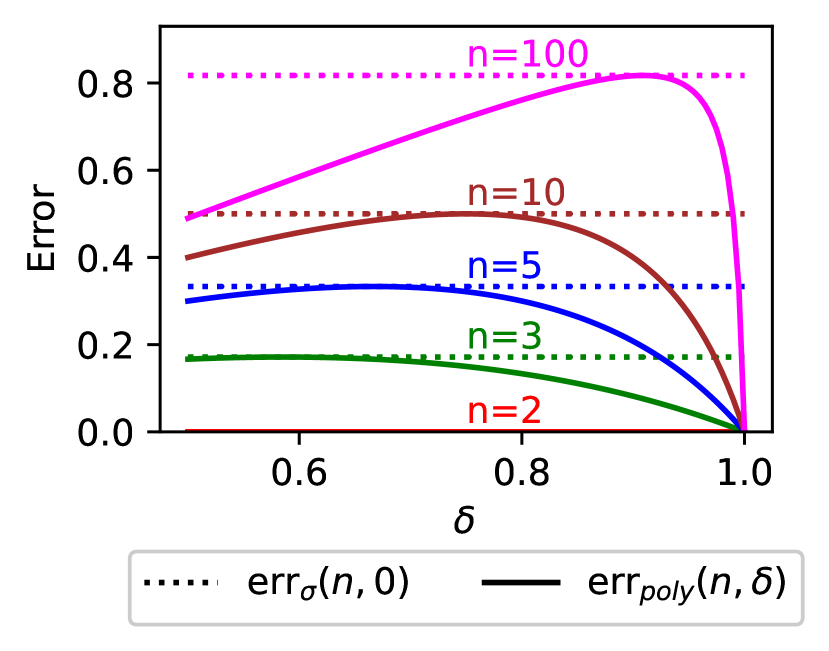
Figure 5: Approximation Errors w.r.t. confidence $\delta$: Ours (solid) and Athavale et al. [2] (dashed).

We assume that $f_{1},f_{2}$ are $\mathrm{ReLU}{}$ NN with one $\mathrm{softmax}$ function after the last layer.Verifying $\delta$-Top-1 equivalence achieves multiple objectives:First, even for larger $Y$ (e.g. intervals over standard deviations for normalized inputs), we may provide meaningful guarantees for a suitable $\delta$.Secondly, we rely on confidence estimates of a component we already trust: The reference NN.Finally, from a technical perspective, constraining the confidence level of $f_{1}$ to $\geq\delta$ while “only” requiring the same classification in $f_{2}$ achieves the asymmetrynecessary for exploiting Differential Verification.Unfortunately, deciding $\delta$-Top-1 equivalence is a coNP-hard decision problem (proof on LABEL:proof:delta_top_1_np):[Complexity of $\delta$-Top-1][end,restate,text link=]Let $Y\subseteq\mathbb{R}^{I}$ be a polytope, $f_{1},f_{2}$ be two $\mathrm{ReLU}{}$-$\mathrm{softmax}$-NN, $\frac{1}{2}<\delta\leq 1$.Deciding whether there exists a $\mathbf{y}\in Y$ and $k\in\left[1,O\right]$ s.t. $\left(f_{1}\left(x\right)\right)_{k}\geq\delta$ but $\exists j\in\left[1,O\right]~{}\left(f_{2}\left(\mathbf{x}\right)\right)_{k}<\left(f_{2}\left(\mathbf{x}\right)\right)_{j}$ is NP-hard. See proof in appendix on page LABEL:proof:prAtEnd\pratendcountercurrent.main-pratenddefaultcategory.texDue to the usage of $\mathrm{softmax}$, the previous NP-membership argument does not apply in this case.To verify $\delta$-Top-1 equivalence, we part from prior work on confidence-based verification [2] and propose the following approximation of all vectors $\mathbf{z}$ for which output $i$ has a confidence $\geq\delta$ (see proof on LABEL:proof:lin_approx_softmax): main-pratenddefaultcategory.tex[Linear approximation of $\mathrm{softmax}$][end,restate,text link=]For $\delta\in\left[1/2,1\right)$ the following set relationship holds:

$$\left\{\mathbf{z}\in\mathbb{R}^{n}~{}\middle|~{}\mathrm{softmax}\left(\mathbf{z}\right)_{i}\geq\delta\right\}\subseteq\left\{\mathbf{z}\in\mathbb{R}^{n}~{}\middle|~{}\bigwedge_{\begin{subarray}{c}j=1\\ j\neq i\end{subarray}}^{n}\mathbf{z}_{i}-\mathbf{z}_{j}\geq\ln\left(\frac{\delta}{1-\delta}\right)\right\}\eqqcolon P_{n}\left(\delta\right)$$

See proof in appendix on page LABEL:proof:prAtEnd\pratendcountercurrent.main-pratenddefaultcategory.texWe can then prove $\delta$-Top-1 equivalence for $\delta\geq\frac{1}{2}$ by reusing the Top-1 Violation LP with $t$ chosen appropriately (see proof on LABEL:proof:soundness_delta_top1):[Soundness for $\delta$-Top-1][end,restate,text link=]Given $\mathcal{Z}{}^{\prime},\mathcal{Z}{}^{\prime\prime},\mathcal{Z}{}^{\Delta}$ from $\textsc{Reach}_{\Delta}$ w.r.t. $Z_{\text{in}}$, $\frac{1}{2}\leq\delta<1$.If for all $k,j\in\left[1,O\right]$ ($k\neq j$) theTop-1 Violation LPs with $t=\ln\left(\frac{\delta}{1-\delta}\right)$ have maxima $\leq 0$, then $f_{2}$ is $\delta$-Top-1 equivalence w.r.t. $f_{1}$ on $\langle Z_{\text{in}}\rangle$. See proof in appendix on page LABEL:proof:prAtEnd\pratendcountercurrent.main-pratenddefaultcategory.texIn comparison to the $\mathrm{softmax}$ approximation by Athavale et al. [2], we approximate via one polytope in the output space (in contrast to a 35-segment piece-wise linear approximation).Additionally, our approximation is parametrized in the confidence threshold $\delta$ while their approximation is uniform across confidence values.We now analyze the precision of the two approximations.Given a desired confidence level $\delta$, we consider its error the maximal deviation below $\delta$ still encompassed by the approximation.For Athavale et al. [2] this maximal error is given as a function $\mathrm{err}_{\sigma}\left(n,\upsilon\right)$ in the input dimension $n$ and the sigmoid approximation error $\upsilon$ (see LABEL:def:max_error_athavale or [2, Thm. 1]).For our approximation, we want to derive the error via the minimal confidence value that is still part of $P_{n}\left(\delta\right)$, i.e. as $\mathrm{err}_{\text{poly}}\left(n,\delta\right)=\delta-\min\left\{\max_{i}\mathrm{softmax}\left(\mathbf{z}\right)_{i}~{}\middle|~{}\mathbf{z}\in P_{n}\left(\delta\right)\right\}$.We can derive the following properties for our approximation error $\mathrm{err}_{\text{poly}}\left(n,\delta\right)$ in relation to the approximation error $\mathrm{err}_{\sigma}\left(n,\upsilon\right)$ incurred by Athavale et al. [2] (proof on LABEL:proof:approx_error):[Maximal Error for our $\mathrm{softmax}$ approximation][end,restate,text link=]Consider $n\geq 2$ and $\delta\geq\frac{1}{2}$, then:

1. $\mathrm{err}_{\text{poly}}\left(n,\delta\right)=\delta\enspace-\enspace\delta/\left(\delta\left(2-n\right)+n-1\right)$ and $\mathrm{err}_{\text{poly}}\left(2,\delta\right)=0$

2. For all $\upsilon>0$ we get $\mathrm{err}_{\sigma}\left(n,\upsilon\right)>\mathrm{err}_{\sigma}\left(n,0\right)=\max_{\delta\in\left[\frac{1}{2},1\right]}\mathrm{err}_{\text{poly}}\left(n,\delta\right)$

3. $\lim_{\delta\to 1}\mathrm{err}_{\text{poly}}\left(n,\delta\right)=0$

See proof in appendix on page LABEL:proof:prAtEnd\pratendcountercurrent.main-pratenddefaultcategory.texNote, that while $\mathrm{err}_{\text{poly}}\left(n,1\right)$ is well defined for $\delta$ the necessary bound $\ln\left(\frac{\delta}{1-\delta}\right)$ is not, i.e. we can only check for $\delta<1$.The observations described in Section 6.0.1 are also observable in Figure 5: By parameterizing the approximation in the confidence threshold $\delta$ we achieve significant precision gains over prior work – independent of output dimensionality ($n$) and in particular as we approach $\delta=1$.

7 Evaluation

We implemented Differential Zonotope verification in a new tool called VeryDiff in Julia [9]. First, we analyze the efficiency of Differential Zonotopes compared to our naive approach for verifying $\varepsilon$ or ($\delta$-)Top-1 equivalence.We also compare the performance of VeryDiff to the previous State-of-the-Art and demonstrate significant performance improvements for $\varepsilon$ and $\delta$-Top-1 equivalence across all benchmark families.LABEL:apx:additional_experimental_results contains an extended evaluation.

Experimental Setup.

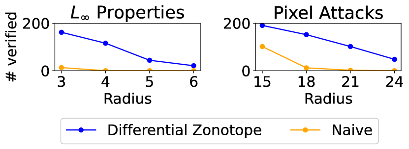
Figure 6: MNIST benchmark queries for which VeryDiff with(out) Differential Zonotopes proves equivalence.

We compare six different tools or configurations on old and new benchmark families.A detailed summary of baselines, benchmark families and NN architectures can be found in LABEL:apx:subsec:eval:setup.For $\varepsilon$ and Top-1 equivalence, we evaluate on preexisting and new ACAS and MNIST NN (airborne collision avoidance and handwritten digit recognition) where the second NN is generated via pruning (and possibly further training).For MNIST, we evaluate w.r.t. input regions generated by Paulsen et al. [31] which prove equivalence on $L_{\infty}$ bounded perturbations of images ($L_{\infty}$ Properties) or targeted pixel perturbations (Pixel Attacks)For $\delta$-Top-1 equivalence, we introduce a new NN verification benchmark for particle jet classification at CERN’s Large Hadron Collider (LHC) [14].We analyze equivalence w.r.t. pruned and further trained NN.NN in this context come with strict real-time requirements making pruned NN highly desirable [14].We verify equivalence for boxes defined via standard deviations over the normalized input space.

7.0.1 Where Differential Verification helps.

We compared VeryDiff with Differential Zonotopes activated to the naive computation without Differential Zonotopes.A summary of all results can be found in LABEL:tab:abelation_diff_zono (LABEL:apx:subsec:eval:abelation).We see significant improvements for $\varepsilon$ equivalence (1430% more instances certified for the MNIST (VeriPrune) benchmark family).Figure 6 breaks down the verified $\varepsilon$ equivalence queries with/without Differential Zonotopes by input radius across all MNIST benchmark queries and shows that Differential Verification helps to verify larger input regions.On the other hand, differential analysis slows down the verification of Top-1 equivalence verification (see LABEL:tab:abelation_diff_zono).We provide a complementary theoretical analysis to this observation in Section 6 and posit this is a fundamental limitation of Differential Verification and not specific to our implementation.In contrast, certification of confidence-based equivalence can profit from Differential Verification across two benchmark families.While we see diminishing speedups as we push the confidence threshold $\delta$ closer to $1$ (implicitly reducing the input space with guarantees), realistic thresholds $\delta>0.5$ (e.g. $0.9$ instead of $1-10^{-7}$) profit most from differential verification (up to speedups of 677 over the naive technique on commonly solved queries for LHC w.r.t. $\delta=0.99$).We found queries where $\varepsilon$ and Top-1 equivalence results differ – underlining the importance of choosing equivalence properties w.r.t. the task at hand.

Table 2: Verification results for $\varepsilon$ and $\delta$-Top-1 equivalence: Speedups for commonly solved instances; improvements reported w.r.t. the best other tool.

Benchmark		Variant	Equiv.		Counterex.		Speedup
							Median	Max
Standard $\varepsilon$ eq.	ACAS	VeryDiff (ours)	150	(+24.0%)	153	(+2.0%)	—	—
		NNEquiv	37		142		37.3	8091.2
		MILPEquiv	16		3		7224.8	36297.0
		Marabou	110		109		141.3	10070.5
		$\alpha,\beta$-CROWN	121		150		15.4	1954.1
	MNIST (VeriPrune)	VeryDiff (ours)	352	(+101.1%)	62	(-43.6%)	—	—
		NNEquiv	0		103		12.6	166.2
		Marabou	10		24		183.9	1390.8
		$\alpha,\beta$-CROWN	175		110		(516.9)	(4220.8)
NeuroDiff $\varepsilon$ eq.	ACAS	VeryDiff (ours)	169	(+39.7%)	161	(+103.8%)	—	—
		NeuroDiff	121		79		43.1	16134.7
	MNIST (VeriPrune)	VeryDiff (ours)	457	(+11.5%)	242	(+404.1%)	—	—
		NeuroDiff	410		48		4.5	1086.8
$\delta$-Top-1	LHC	VeryDiff (ours)	77	(327.8%)	—		—	—
		$\alpha,\beta$-CROWN	18		—		324.5	11274.3

7.0.2 $\varepsilon$ Equivalence.

We compare our tool with other $\varepsilon$ equivalence verification techniques from the literature and summarize the results in Table 2.Across both benchmarks from prior literature (ACAS and MNIST), we significantly outperform equivalence-specific verifiers (NNEquiv [36], MILPEquiv [25], NeuroDiff [31]) as well as general NN verification techniques ($\alpha,\beta$-CROWN [zhang2018efficient, xu2020automatic, xu2021fast, 40, zhang22babattack, zhang2022general, 33, 26], Marabou [24, 42]) for certification of equivalence.$\alpha,\beta$-CROWN outperforms VeryDiff in the search for counterexamples.We suspect this is due to its adversarial attack techniques [zhang22babattack].Due to incompatible differences in the property checked by NeuroDiff’s implementation (see LABEL:apx:subsec:eval:setup), we performed a separate comparison where VeryDiff outperforms NeuroDiff on the same property.

7.0.3 $\delta$-Top-1 Equivalence.

Differential Verification significantly improves upon the generic State-of-the-Art NN verifier $\alpha,\beta$-CROWN (see Table 2).We concede that $\alpha,\beta$-CROWN’s attack techniques outperform VeryDiff’s counterexample generation (see $\varepsilon$ equivalence).Hence, our evaluation focuses on equivalence certification.The objective for $\delta$-Top-1 equivalence is to provide guarantees for low values $\delta$.$\alpha,\beta$-CROWN was only able to provide guarantees for 10 of the NN in the benchmark set.In each case, VeryDiff was able to prove equivalence for lower (i.e. better) or equal $\delta$ values.For the 3 NN where the provided guarantees of $\alpha,\beta$-CROWN and VeryDiff matched, both tools only verified equivalence for $\delta=1-10^{-7}$, i.e. they provided an extremely limited guarantee.This underlines that VeryDiff is a significant step forward in the verification of $\delta$-Top-1 equivalence.

7.0.4 Limitations

Larger weight differences between NN and accumulating $\mathrm{ReLU}{}$ approximations may decrease speedups achievable via Differential Verification (see discussion in LABEL:apx:subsec:eval:confidence).Nonetheless, VeryDiff outperforms alternative verifiers – often by orders of magnitude.Another limitation for confidence-based NN verification is the possibility of satisfied for high confidence thresholds (for mitigation via calibration [18, 1] see Athavale et al. [2]).However, for equivalence verification, we consider the reference NN $f_{1}$ (incl. its confidence) trustworthy.

8 Conclusion

We introducedDifferential Zonotopes as an abstract domain for NN equivalence verification.Our extensive evaluation shows that we outperform the Differential Verification tool NeuroDiff [30, 31]) as well as State-of-the-Art NN verifiers.Moreover, our paper provides insights into the circumstances where differential reasoning does (not) aid verification.As discussed in Sections 6 and 7, whether Differential Verification helps is not always straightforward for specifications involving classification.We believe that confidence-based equivalence is the way forward to scale equivalence verification beyond tiny input regions such as $\epsilon$-balls criticized in the literature [17].Finally, we introduced a simpler approximation for $\mathrm{softmax}$ that is provably tighter than prior work [2].

Future Work.

We see potential in extending generic NN verifiers (e.g. Marabou’s network level reasoner [42]) with differential abstract domains to improve their reasoning capabilities for relational properties.

References

- [1] Ao, S., Rueger, S., Siddharthan, A.: Two sides of miscalibration: Identifyingover and under-confidence prediction for network calibration. In: Evans,R.J., Shpitser, I. (eds.) Uncertainty in Artificial Intelligence, UAI 2023,July 31 - 4 August 2023, Pittsburgh, PA, USA. Proceedings of MachineLearning Research, vol. 216, pp. 77–87. PMLR (2023),https://proceedings.mlr.press/v216/ao23a.html
- [2] Athavale, A., Bartocci, E., Christakis, M., Maffei, M., Nickovic, D.,Weissenbacher, G.: Verifying global two-safety properties in neural networkswith confidence. In: Gurfinkel, A., Ganesh, V. (eds.) Computer AidedVerification - 36th International Conference, CAV 2024, Montreal, QC,Canada, July 24-27, 2024, Proceedings, Part II. LNCS, vol. 14682, pp.329–351. Springer (2024). https://doi.org/10.1007/978-3-031-65630-9_17
- [3] Bak, S.: nnenum: Verification of relu neural networks with optimizedabstraction refinement. In: Dutle, A., Moscato, M.M., Titolo, L.,Muñoz, C.A., Perez, I. (eds.) NASA Formal Methods - 13thInternational Symposium, NFM 2021, Virtual Event, May 24-28, 2021,Proceedings. LNCS, vol. 12673, pp. 19–36. Springer (2021).https://doi.org/10.1007/978-3-030-76384-8_2
- [4] Bak, S., Brix, C., Johnson, T., Liu, C., Wu, H.: VNN-COMP 2024 (2024),https://docs.google.com/presentation/d/1RvZWeAdTfRC3bNtCqt84O6IIPoJBnF4jnsEvhTTxsPE/edit?usp=sharing,accessed: 10/04/2024
- [5] Bak, S., Tran, H., Hobbs, K., Johnson, T.T.: Improved geometric pathenumeration for verifying ReLU neural networks. In: Lahiri, S.K., Wang, C.(eds.) Computer Aided Verification - 32nd International Conference, CAV2020, Los Angeles, CA, USA, July 21-24, 2020, Proceedings, Part I. LNCS,vol. 12224, pp. 66–96. Springer (2020). https://doi.org/10.1007/978-3-030-53288-8_4
- [6] Banerjee, D., Singh, G.: Relational DNN verification with cross executionalbound refinement. In: Forty-first International Conference on MachineLearning (2024), https://openreview.net/forum?id=HOG80Yk4Gw
- [7] Banerjee, D., Xu, C., Singh, G.: Input-relational verification of deep neuralnetworks. Proc. ACM Program. Lang. 8(PLDI), 1–27 (2024).https://doi.org/10.1145/3656377
- [8] Barthe, G., Crespo, J.M., Kunz, C.: Relational verification using productprograms. In: Butler, M.J., Schulte, W. (eds.) FM 2011: Formal Methods -17th International Symposium on Formal Methods, Limerick, Ireland, June20-24, 2011. Proceedings. LNCS, vol. 6664, pp. 200–214. Springer (2011).https://doi.org/10.1007/978-3-642-21437-0_17
- [9] Bezanson, J., Edelman, A., Karpinski, S., Shah, V.B.: Julia: A fresh approachto numerical computing. SIAM Rev. 59(1), 65–98 (2017).https://doi.org/10.1137/141000671, https://doi.org/10.1137/141000671
- [10] Brix, C., Müller, M.N., Bak, S., Johnson, T.T., Liu, C.: First threeyears of the international verification of neural networks competition(VNN-COMP). Int. J. Softw. Tools Technol. Transf. 25(3),329–339 (2023). https://doi.org/10.1007/S10009-023-00703-4
- [11] Cinar, I., Koklu, M.: Classification of rice varieties using artificialintelligence methods. International Journal of Intelligent Systems andApplications in Engineering 7(3), 188–194 (2019)
- [12] Cook, S.A.: The complexity of theorem-proving procedures. In: Harrison, M.A.,Banerji, R.B., Ullman, J.D. (eds.) Proceedings of the 3rd Annual ACMSymposium on Theory of Computing, May 3-5, 1971, Shaker Heights, Ohio, USA.pp. 151–158. ACM (1971). https://doi.org/10.1145/800157.805047
- [13] Demarchi, S., Guidotti, D., Pulina, L., Tacchella, A.: Supportingstandardization of neural networks verification with vnnlib and coconet. In:Narodytska, N., Amir, G., Katz, G., Isac, O. (eds.) Proceedings of the 6thWorkshop on Formal Methods for ML-Enabled Autonomous Systems. KalpaPublications in Computing, vol. 16, pp. 47–58. EasyChair (2023).https://doi.org/10.29007/5pdh, /publications/paper/Qgdn
- [14] Duarte, J., Han, S., Harris, P., Jindariani, S., Kreinar, E., Kreis, B.,Ngadiuba, J., Pierini, M., Rivera, R., Tran, N., Wu, Z.: Fast inference ofdeep neural networks in fpgas for particle physics. Journal ofInstrumentation 13(07), P07027 (jul 2018).https://doi.org/10.1088/1748-0221/13/07/P07027
- [15] Eleftheriadis, C., Kekatos, N., Katsaros, P., Tripakis, S.: On neural networkequivalence checking using SMT solvers. In: Bogomolov, S., Parker, D.(eds.) Formal Modeling and Analysis of Timed Systems - 20th InternationalConference, FORMATS 2022, Warsaw, Poland, September 13-15, 2022,Proceedings. LNCS, vol. 13465, pp. 237–257. Springer (2022).https://doi.org/10.1007/978-3-031-15839-1_14
- [16] Gehr, T., Mirman, M., Drachsler-Cohen, D., Tsankov, P., Chaudhuri, S.,Vechev, M.T.: AI2: safety and robustness certification of neural networkswith abstract interpretation. In: 2018 IEEE Symposium on Security andPrivacy, SP 2018, Proceedings, 21-23 May 2018, San Francisco, California,USA. pp. 3–18. IEEE Computer Society (2018). https://doi.org/10.1109/SP.2018.00058
- [17] Geng, C., Le, N., Xu, X., Wang, Z., Gurfinkel, A., Si, X.: Towards reliableneural specifications. In: Krause, A., Brunskill, E., Cho, K., Engelhardt,B., Sabato, S., Scarlett, J. (eds.) International Conference on MachineLearning, ICML 2023, 23-29 July 2023, Honolulu, Hawaii, USA. Proceedingsof Machine Learning Research, vol. 202, pp. 11196–11212. PMLR (2023),https://proceedings.mlr.press/v202/geng23a.html
- [18] Guo, C., Pleiss, G., Sun, Y., Weinberger, K.Q.: On calibration of modern neuralnetworks. In: Precup, D., Teh, Y.W. (eds.) Proceedings of the 34thInternational Conference on Machine Learning, ICML 2017, Sydney, NSW,Australia, 6-11 August 2017. Proceedings of Machine Learning Research,vol. 70, pp. 1321–1330. PMLR (2017),http://proceedings.mlr.press/v70/guo17a.html
- [19] Gurobi Optimization, LLC: Gurobi Optimizer Reference Manual (2023),https://www.gurobi.com
- [20] Habeeb, P., Prabhakar, P.: Approximate conformance verification of deep neuralnetworks. In: Benz, N., Gopinath, D., Shi, N. (eds.) NASA Formal Methods -16th International Symposium, NFM 2024, Moffett Field, CA, USA, June 4-6,2024, Proceedings. LNCS, vol. 14627, pp. 223–238. Springer (2024).https://doi.org/10.1007/978-3-031-60698-4_13
- [21] Julian, K.D., Lopez, J., Brush, J.S., Owen, M.P., Kochenderfer, M.J.: Policycompression for aircraft collision avoidance systems. In: AIAA/IEEEDigital Avionics Systems Conference - Proceedings. vol. 2016-Decem,pp. 1–10. IEEE (2016). https://doi.org/10.1109/DASC.2016.7778091, iSSN: 21557209
- [22] Karmarkar, N.: A new polynomial-time algorithm for linear programming. In:DeMillo, R.A. (ed.) Proceedings of the 16th Annual ACM Symposium on Theoryof Computing, April 30 - May 2, 1984, Washington, DC, USA. pp. 302–311.ACM (1984). https://doi.org/10.1145/800057.808695
- [23] Katz, G., Barrett, C.W., Dill, D.L., Julian, K., Kochenderfer, M.J.: Reluplex:An efficient SMT solver for verifying deep neural networks. In: Majumdar,R., Kuncak, V. (eds.) Computer Aided Verification - 29th InternationalConference, CAV 2017, Heidelberg, Germany, July 24-28, 2017, Proceedings,Part I. LNCS, vol. 10426, pp. 97–117. Springer (2017).https://doi.org/10.1007/978-3-319-63387-9_5
- [24] Katz, G., Huang, D.A., Ibeling, D., Julian, K., Lazarus, C., Lim, R., Shah, P.,Thakoor, S., Wu, H., Zeljic, A., Dill, D.L., Kochenderfer, M.J., Barrett,C.W.: The Marabou framework for verification and analysis of deep neuralnetworks. In: Dillig, I., Tasiran, S. (eds.) Computer Aided Verification -31st International Conference, CAV 2019, New York City, NY, USA, July15-18, 2019, Proceedings, Part I. LNCS, vol. 11561, pp. 443–452. Springer(2019). https://doi.org/10.1007/978-3-030-25540-4_26
- [25] Kleine Büning, M., Kern, P., Sinz, C.: Verifying equivalence propertiesof neural networks with ReLU activation functions. In: Simonis, H. (ed.)Principles and Practice of Constraint Programming - 26th InternationalConference, CP 2020, Louvain-la-Neuve, Belgium, September 7-11, 2020,Proceedings. LNCS, vol. 12333, pp. 868–884. Springer (2020).https://doi.org/10.1007/978-3-030-58475-7_50
- [26] Kotha, S., Brix, C., Kolter, J.Z., Dvijotham, K., Zhang, H.: Provably boundingneural network preimages. In: Oh, A., Naumann, T., Globerson, A., Saenko, K.,Hardt, M., Levine, S. (eds.) Advances in Neural Information ProcessingSystems 36: Annual Conference on Neural Information Processing Systems 2023,NeurIPS 2023, New Orleans, LA, USA, December 10 - 16, 2023 (2023),http://papers.nips.cc/paper_files/paper/2023/hash/fe061ec0ae03c5cf5b5323a2b9121bfd-Abstract-Conference.html
- [27] Matos, J.B.P., Filho, E.B.d.L., Bessa, I., Manino, E., Song, X., Cordeiro,L.C.: Counterexample guided neural network quantization refinement. IEEETransactions on Computer-Aided Design of Integrated Circuits and Systemspp. 1–1 (2023). https://doi.org/10.1109/TCAD.2023.3335313
- [28] Müller, C., Serre, F., Singh, G., Püschel, M., Vechev, M.T.:Scaling polyhedral neural network verification on gpus. In: Smola, A.,Dimakis, A., Stoica, I. (eds.) Proceedings of the Fourth Conference onMachine Learning and Systems, MLSys 2021, virtual, April 5-9, 2021. mlsys.org(2021),https://proceedings.mlsys.org/paper_files/paper/2021/hash/7c98f9c7ab2df90911da23f9ce72ed6e-Abstract.html
- [29] Narodytska, N., Kasiviswanathan, S.P., Ryzhyk, L., Sagiv, M., Walsh, T.:Verifying properties of binarized deep neural networks. In: McIlraith, S.A.,Weinberger, K.Q. (eds.) Proceedings of the Thirty-Second AAAI Conference onArtificial Intelligence, AAAI-18, New Orleans, Louisiana, USA, February2-7, 2018. pp. 6615–6624. AAAI Press (2018).https://doi.org/10.1609/AAAI.V32I1.12206
- [30] Paulsen, B., Wang, J., Wang, C.: Reludiff: differential verification of deepneural networks. In: Rothermel, G., Bae, D. (eds.) ICSE ’20: 42ndInternational Conference on Software Engineering, Seoul, South Korea, 27 June- 19 July, 2020. pp. 714–726. ACM (2020). https://doi.org/10.1145/3377811.3380337
- [31] Paulsen, B., Wang, J., Wang, J., Wang, C.: NeuroDiff: scalable differentialverification of neural networks using fine-grained approximation. In: 35thIEEE/ACM International Conference on Automated Software Engineering, ASE2020, Melbourne, Australia, September 21-25, 2020. pp. 784–796. IEEE(2020). https://doi.org/10.1145/3324884.3416560
- [32] Sälzer, M., Lange, M.: Reachability is np-complete even for the simplestneural networks. In: Bell, P.C., Totzke, P., Potapov, I. (eds.) ReachabilityProblems - 15th International Conference, RP 2021, Liverpool, UK, October25-27, 2021, Proceedings. LNCS, vol. 13035, pp. 149–164. Springer (2021).https://doi.org/10.1007/978-3-030-89716-1_10
- [33] Shi, Z., Jin, Q., Kolter, Z., Jana, S., Hsieh, C., Zhang, H.: Neural networkverification with branch-and-bound for general nonlinearities. CoRRabs/2405.21063 (2024). https://doi.org/10.48550/ARXIV.2405.21063,https://doi.org/10.48550/arXiv.2405.21063
- [34] Shriver, D., Elbaum, S.G., Dwyer, M.B.: DNNV: A framework for deep neuralnetwork verification. In: Silva, A., Leino, K.R.M. (eds.) Computer AidedVerification - 33rd International Conference, CAV 2021, Virtual Event, July20-23, 2021, Proceedings, Part I. LNCS, vol. 12759, pp. 137–150. Springer(2021). https://doi.org/10.1007/978-3-030-81685-8_6
- [35] Singh, G., Gehr, T., Mirman, M., Püschel, M., Vechev, M.T.: Fast andeffective robustness certification. In: Bengio, S., Wallach, H.M.,Larochelle, H., Grauman, K., Cesa-Bianchi, N., Garnett, R. (eds.) Advancesin Neural Information Processing Systems 31: Annual Conference on NeuralInformation Processing Systems 2018, NeurIPS 2018, December 3-8, 2018,Montréal, Canada. pp. 10825–10836 (2018),https://proceedings.neurips.cc/paper/2018/hash/f2f446980d8e971ef3da97af089481c3-Abstract.html
- [36] Teuber, S., Büning, M.K., Kern, P., Sinz, C.: Geometric path enumerationfor equivalence verification of neural networks. In: 33rd IEEEInternational Conference on Tools with Artificial Intelligence, ICTAI 2021,Washington, DC, USA, November 1-3, 2021. pp. 200–208. IEEE (2021).https://doi.org/10.1109/ICTAI52525.2021.00035
- [37] Tran, H., Lopez, D.M., Musau, P., Yang, X., Nguyen, L.V., Xiang, W., Johnson,T.T.: Star-based reachability analysis of deep neural networks. In: ter Beek,M.H., McIver, A., Oliveira, J.N. (eds.) Formal Methods - The Next 30 Years -Third World Congress, FM 2019, Porto, Portugal, October 7-11, 2019,Proceedings. LNCS, vol. 11800, pp. 670–686. Springer (2019).https://doi.org/10.1007/978-3-030-30942-8_39
- [38] Wang, S., Pei, K., Whitehouse, J., Yang, J., Jana, S.: Efficient formal safetyanalysis of neural networks. In: Bengio, S., Wallach, H.M., Larochelle, H.,Grauman, K., Cesa-Bianchi, N., Garnett, R. (eds.) Advances in NeuralInformation Processing Systems 31: Annual Conference on Neural InformationProcessing Systems 2018, NeurIPS 2018, December 3-8, 2018, Montréal,Canada. pp. 6369–6379 (2018),https://proceedings.neurips.cc/paper/2018/hash/2ecd2bd94734e5dd392d8678bc64cdab-Abstract.html
- [39] Wang, S., Pei, K., Whitehouse, J., Yang, J., Jana, S.: Formal security analysisof neural networks using symbolic intervals. In: Enck, W., Felt, A.P. (eds.)27th USENIX Security Symposium, USENIX Security 2018, Baltimore, MD, USA,August 15-17, 2018. pp. 1599–1614. USENIX Association (2018),https://www.usenix.org/conference/usenixsecurity18/presentation/wang-shiqi
- [40] Wang, S., Zhang, H., Xu, K., Lin, X., Jana, S., Hsieh, C., Kolter, J.Z.:Beta-crown: Efficient bound propagation with per-neuron split constraints forcomplete and incomplete neural network verification. CoRRabs/2103.06624 (2021), https://arxiv.org/abs/2103.06624
- [41] Wang, W., Wang, K., Cheng, Z., Yang, Y.: Veriprune: Equivalence verification ofnode pruned neural network. Neurocomputing 577, 127347 (2024).https://doi.org/https://doi.org/10.1016/j.neucom.2024.127347,https://www.sciencedirect.com/science/article/pii/S0925231224001188
- [42] Wu, H., Isac, O., Zeljic, A., Tagomori, T., Daggitt, M.L., Kokke, W., Refaeli,I., Amir, G., Julian, K., Bassan, S., Huang, P., Lahav, O., Wu, M., Zhang,M., Komendantskaya, E., Katz, G., Barrett, C.W.: Marabou 2.0: A versatileformal analyzer of neural networks. In: Gurfinkel, A., Ganesh, V. (eds.)Computer Aided Verification - 36th International Conference, CAV 2024,Montreal, QC, Canada, July 24-27, 2024, Proceedings, Part II. LNCS, vol.14682, pp. 249–264. Springer (2024). https://doi.org/10.1007/978-3-031-65630-9