Leveraging Graph Neural Networks and Multi-Agent Reinforcement Learning for Inventory Control in Supply Chains

Abstract

Inventory control in modern supply chains has attracted significant attention due to the increasing number of disruptive shocks and the challenges posed by complex dynamics, uncertainties, and limited collaboration. Traditional methods, which often rely on static parameters, struggle to adapt to changing environments. This paper proposes a Multi-Agent Reinforcement Learning (MARL) framework with Graph Neural Networks (GNNs) for state representation to address these limitations.

Our approach redefines the action space by parameterizing heuristic inventory control policies, making it adaptive as the parameters dynamically adjust based on system conditions. By leveraging the inherent graph structure of supply chains, our framework enables agents to learn the system’s topology, and we employ a centralized learning, decentralized execution scheme that allows agents to learn collaboratively while overcoming information-sharing constraints. Additionally, we incorporate global mean pooling and regularization techniques to enhance performance.

We test the capabilities of our proposed approach on four different supply chain configurations and conduct a sensitivity analysis. This work paves the way for utilizing MARL-GNN frameworks to improve inventory management in complex, decentralized supply chain environments.

organization=Imperial College London,addressline=Department of Chemical Engineering, city=London, postcode=SW7 2AZ

1 Introduction

Modern supply chains are complex and operate under uncertain environments. These uncertainties can lead to disruptions and sub-optimal performance, often due to operational failures or poor coordination between different parts of the supply chain. The inventory control problem, a sequential decision-making problem, is additionally challenged by stochastic and volatile factors such as lead times and seasonal demand patterns, often resulting in sub-optimal performance. The impact of disruptions such as the bullwhip (demand amplification) or ripple effect (disruption propagation) effect can be alleviated through collaborative efforts among different entities within a supply chain (de Almeida et al., 2015).

1.1 Inventory Control

The theory of inventory control can be traced back to the news-vendor problem (Edgeworth, 1888; Clark and Scarf, 1960), and the first widely used numerical solutions for inventory optimization seems to be the Economic Order Quantity (EOQ) model (Erlenkotter, 1990). These works were fundamental to the widely known policies in inventory control theory: (R,S), (s,S), (R,s,S) and (R,Q) (Federgruen and Zheng, 1992; Silver et al., 1998). Over the years, control theory has had an influence on production planning and inventory control (Aggarwal, 1974; Jackson et al., 2020). The complexity of modern systems has driven dynamic programming applications, unfortunately, obtaining exact analytical solutions often proves infeasible due to computational demands (Bellman, 1952). This has fuelled the adoption of advanced techniques beyond traditional closed-form solutions. On one hand, stochastic (Küçükyavuz, 2011) and distributionally-robust optimization approaches (Bertsimas et al., 2019; Qiu et al., 2021), while promising, face challenges such as online tractability, limiting their practical applicability in real-world supply chain scenarios. On the other hand, traditional approaches leveraging heuristics, while offering a simpler implementation, struggle to adapt to the dynamic and complex nature of modern supply chains.

1.2 Reinforcement learning for Inventory Control

Reinforcement learning (RL) has emerged as a promising alternative for addressing the challenges of stochastic sequential decision-making problems. Its ability to excel in complex, dynamic environments and handle uncertainty, places RL as a valuable tool to enhance decision making in supply chains. While closely linked to dynamic programming, RL offers a general solution to identify approximate optimal policies for stochastic processes by leveraging the Bellman optimality equation to iteratively update value functions and improve decision-making policies over time. RL also provides a cost-effective solution for decision-making by enabling offline training, which reduces the online computational overhead compared to optimization approaches that require continual updates in receding or shrinking horizon frameworks. However, RL’s effectiveness relies on the availability of information sharing among the entities within the supply chain. In scenarios where multiple interconnected entities are involved, ensuring seamless information exchange can be challenging due to factors such as data privacy concerns, proprietary information, or communication constraints. This limitation may hinder the adoption and implementation of RL-based approaches in complex supply chain environments, highlighting the need for strategies to address information sharing challenges effectively.

1.3 Multi-Agent Reinforcement Learning

This challenge in information sharing motivates the exploration of multi-agent reinforcement learning (MARL) approaches in supply chain management. MARL frameworks allow multiple entities within a supply chain to autonomously learn and adapt their decision-making processes while interacting with each other. By leveraging MARL, supply chain entities can collaborate and coordinate their actions more effectively, leading to improved overall performance and resilience against disruptions. Additionally, MARL provides a scalable approach to handle the complexities of large-scale supply chain systems by distributing decision-making across multiple agents.

However, despite its potential, MARL faces several challenges. One issue is the non-stationarity of the learning environment inherent in MARL (Tan, 1993; Tampuu et al., 2017). This occurs when multiple agents are learning simultaneously so the transition dynamics are not stationary. One setting commonly used to overcome this is to use a central critic during training that has access to global observations and actions (Nekoei et al., 2023). This is known as the Centralised Training, Decentralized Execution learning paradigm. However, while adding more information can help mitigate the non-stationarity problem, it can also lead to new issues. Naively concatenating all available information can result in information overload and inefficiencies (Lowe et al., 2017; Yu et al., 2022; Nayak et al., 2023). This indiscriminate accumulation of data can cause policy overfitting, where agents develop strategies that perform well on the excessive training information but poorly in real-world scenarios due to the lack of generalization (Nayak et al., 2023; Hu et al., 2021). Therefore, the development of novel techniques for smart information aggregation is required to avoid policy overfitting and enhance the efficacy of MARL frameworks in supply chain management.

1.4 Related Work

Given the inherent complexity and uncertainty in inventory management systems, there are several approaches that address specific challenges within this domain. In this section, we highlight some related previous work and methodologies tackling the inventory management problem.

One example to find optimal inventory control policies is using traditional heuristics. These are simple, exact methods which suit relatively simple problems. Common examples include reorder point heuristics (Federgruen and Zheng, 1992; Silver et al., 1998) or the Economic Order Quantity model (Erlenkotter, 1990). However, a key limitation of these heuristics is their lack of adaptability. They rely on pre-defined parameters that may not be effective in dynamic environments with fluctuating demand or unforeseen circumstances.

Moreover, inventory management problems can also be tackled using optimization techniques like Linear Programming (LP) (Janssens and Ramaekers, 2011) or Mixed-Integer Linear Programming (MILP) (You and Grossmann, 2008). LP is well-suited for problems with linear relationships, while MILP offers more flexibility by incorporating integer variables to address specific complexities like minimum order quantities. However, these methods do not directly account for uncertainty.

If the optimal policy is analytically intractable, methods like stochastic optimization can be used to find an approximate optimal policy (Grossmann et al., 2016; You and Grossmann, 2011). While stochastic optimization often finds good solutions, it does not guarantee optimality. In specific scenarios, exact numerical methods like dynamic programming might be applicable (Berovic and Vinter, 2004; Perez et al., 2021). However, these methods are often limited by scale due to computational demands. This leads to approximate numerical methods. These methods provide scalability but may be at a sub-optimal performance. Additionally, Approximate Dynamic Programming (ADP) is a powerful technique specifically designed for problems with both dynamics (e.g., decisions impact future states) and stochasticity (e.g., uncertain outcomes) (Katanyukul et al., 2011). ADP leverages approximations and sampling techniques to find good solutions for complex inventory management problems that might be intractable for traditional methods. Reinforcement Learning methods, closely related to dynamic programming, also belong to the approximate numerical methods class.

Reinforcement learning has emerged as a promising approach to address the dynamic and complex nature of inventory management systems (Giannoccaro and Pontrandolfo, 2002; Bharti et al., 2020a; Boute et al., 2022; Rangel-Martinez and Ricardez-Sandoval, 2024). Single-Agent RL methodologies have been explored extensively in this context to solve a Markov Decision Process (MDP), the mathematical framework used to model decision making in an inventory management system. Unlike traditional heuristic approaches that rely on pre-defined rules, RL leverages interaction with the environment to learn optimal policies. Reinforcement learning, particularly deep reinforcement learning, leverages neural networks to approximate the value functions and policies, enabling it to handle high-dimensional state and action spaces. Methods like Q-learning (Chaharsooghi et al., 2008; Kara and Dogan, 2018; Bharti et al., 2020b; Vera, 2021), Deep Q-Networks (DQN) (Oroojlooyjadid et al., 2022; Meisheri et al., 2020), and Policy Gradient methods (Stranieri and Stella, 2022; Siems et al., 2023; Burtea and Tsay, 2024) have shown promise in developing adaptive and scalable inventory policies that can learn from interactions with the environment over time. However, RL often struggles with integer or mixed-integer decisions, which are common in inventory management problems (e.g., order quantities). As the scale of inventory systems increases, the complexity of the decision-making process grows, resulting in a significantly larger action space. This increased complexity can hinder the effectiveness of RL algorithms, as they require extensive training data and longer convergence times to identify optimal policies. This limitation is particularly relevant because studies using RL for inventory control often represent the act of order replenishment as a discrete integer decision Chaharsooghi et al. (2008); Stranieri and Stella (2022), rather than leveraging pre-defined heuristic parameters like reorder point (s) or order-up-to level (S) which could speed up adoption in industry.

There has been a growing interest to leverage the graph structure of a supply chain by using Graph Neural Networks (GNNs). The main idea is to leverage GNNs to learn the hidden representation of the data encoded as a graph structure (Munikoti et al., 2022). This allows RL agents to efficiently adapt to changes in the problem domain. The application of GNNs to RL has been widely studied for a series of well known combinatorial optimization problems (Khalil et al., 2017; Mazyavkina et al., 2021) such as the vehicle routing problem (Munikoti et al., 2022), travel salesman problem (Munikoti et al., 2022) and the job shop scheduling problem (Zhang et al., 2020a, b). GNNs have been shown to improve performance across different graph sizes and types. These works provide an initial foundation but they consider simplified supply chain instances with deterministic lead times and assume centralized information. Unfortunately, real-world supply chains face inherent information sharing constraints. These constraints can arise due to technical limitations caused by incompatible systems, the inherent complex nature of supply chain structures, or even due to privacy concerns about sharing sensitive data.

To address these limitations and leverage the collaborative nature of supply chains, multi-agent RL approaches have gained significant momentum but remain limited. These approaches model multiple agents, each representing a decision-maker within the supply chain, and allow them to interact and learn from each other. The application of MARL to the inventory management problem is relatively limited compared to other domains including single-agent RL. However, there is growing recognition of the potential benefits of MARL in addressing the dynamic and collaborative nature of inventory management in multi-agent environments. Liu et al. (2022b) applied Heterogeneous-Agent Proximal Policy Optimization (HAPPO) to a serial supply chain which showed overall better performance than single-agent RL. The study also concluded that information sharing between entities helps alleviate the bullwhip effect. Another study conducted by (Feng et al., 2022b), applied a Decentralized PPO framework on a single store problem with a large number of stock keeping units. This approach accelerated policy learning compared to standard MARL algorithm. Additionally, (Khirwar et al., 2023) applied a PPO variation MARL framework to a multi-echelon environment, and it outperformed other base-stock policies. Sultana et al. (2020), applied a multi-agent advantage actor critic algorithm to a multi-echelon, multi-product system but assumed a lead time of zero. Finally, Mousa et al. (2023) provided an analysis of multi-agent reinforcement learning algorithms for decentralised inventory management systems. The study showed that MAPPO outperformed other MARL methods and further highlighted MARL as a promising decentralized control solution for large-scale stochastic systems. While these studies presented in inventory management have made progress in applying MARL techniques, there are still opportunities for improvement. One area deserving further attention is how to leverage the inherent graph structure of a supply chain to enhance RL frameworks’ performance. By exploiting the connectivity and dependencies between different supply chain nodes, we can develop more effective algorithms that address the complexities of multi-agent inventory management.

1.5 Motivation

In this work, we propose leveraging the capabilities of GNNs to learn hidden representations of agents and their interactions. These representations are then integrated into a MARL framework to find optimal inventory policies in a multi-echelon supply chain network. Our contributions are summarized as follows:

• We propose the redefinition of the action space from order replenishment to parametrize a heuristic inventory control policy where both parameters can be dynamically adjusted based on current system dynamics. This ensures early adoption of new optimization techniques due to its interpretability whilst accommodating real-world complexities. Moreover, by focusing on parameterized heuristics, we can effectively navigate the challenges that RL faces with integer decisions, such as those related to order quantities.

• We leverage the inherent graph structure of a supply chain to aid collaboration between entities in a supply chain.

• We reduce dimensionality and increase scalability of a MARL-GNN framework by incorporating a global mean pooling aggregation mechanism within our algorithmic framework.

• We introduce Gaussian perturbations into the value function and perform a sensitivity analysis on the perturbation intensity to reduce policy overfitting and address potential distributional shift, serving as a regularization technique.

• We demonstrate the effectiveness of our method in terms of scalability through four multi-echelon supply chain scenarios.

The rest of this paper is organized as follows: Section 2 provides the background on multi-agent reinforcement learning, Section 3 describes our proposed decentralized decision-making framework in more detail, Section 4 discusses the experimental results obtained and finally Section 5 concludes this paper and provides an outlook for future work.

2 Preliminaries

We first provide a background into the components that contribute towards our methodology including single agent Proximal Policy Optimisation (PPO) and the multi-agent extensions of PPO.

2.1 Single Agent Reinforcement Learning - PPO

Proximal Policy Optimisation (PPO) is a popular first-order, on-policy single agent reinforcement learning method. PPO is an actor-critic algorithm where a policy $\pi_{\theta}$ and value function $V_{\phi}(s)$ are two separate neural networks parameterised by $\theta$ and $\phi$ respectively. In actor critic algorithms like PPO, $V_{\phi}(s)$ is introduced to reduce the variance but may introduce a bias in $\pi_{\theta}$. The two variations of PPO are using a penalty function or a clipping function. The later is known to be crucial for its performance as the clipping function constraints the ratio between the new and old policy within a certain range to prevent large policy updates that may lead to instability.
The PPO policy loss can be defined as:

$$\mathcal{L}_{\theta}=\mathbb{E}_{(s_{t},a_{t})\sim\pi_{\theta_{old}}}\left[\min\biggl{(}\frac{\pi_{\theta}(a_{t}|s_{t})}{\pi_{\theta_{old}}(a_{t}|s_{t})}A_{t},\text{clip}\biggl{(}\frac{\pi_{\theta}(a_{t}|s_{t})}{\pi_{\theta_{old}}(a_{t}|s_{t})},1-\epsilon,1+\epsilon\biggr{)}A_{t}\biggr{)}\right]$$ (1)

where $\pi_{\theta}(a_{t}|s_{t})$ represents the probability of taking actions $a_{t}$ in state $s_{t}$ under the current policy parameterized by $\theta$, $\pi_{\theta_{old}}(a_{t}|s_{t})$ is fixed during the policy update step and represents the probability of taking action $a_{t}$ in state $s_{t}$ under the old policy (from the previous iteration) parameterized by $\theta_{\text{old}}$, $a_{t}$ and $s_{t}$ are the action and state respectively taken at time step $t$, $\epsilon$ represents a hyperparameter that determines how much the new policy can deviate from the old policy and $\text{clip}(\cdot,1-\epsilon,1+\epsilon)$ is the clipping function that constraints the ratio of the new to old policy’s probabilities within a certain range which prevents the policy from making overly large updates that could lead to instability. Finally, $A_{t}$ is the advantage function defined as:

$$A_{t}=R_{t}+\gamma V_{\phi}(s_{t+1})-V_{\phi}(s_{t})$$ (2)

where $R_{t}$ and $V_{\phi}(s_{t})$ is the reward and value function at time step $t$ respectively and $\gamma$ is the discount factor. The general advantage estimation (GAE), used to compute the advantage, is given by:

$$\hat{A}_{t}^{\textbf{GAE}}=\sum_{l=0}^{\infty}(\gamma\lambda)^{l}\delta_{t+l}$$ (3)

where the variable $l$ represents the index of the future time step relative to the current time step $t$. This summation captures the discounted temporal difference (TD) errors, $\delta_{t+l}$, where $\delta_{t+l}=R_{t+l}+\gamma V(s_{t+l+1})-V(s_{t+l})$ is the TD error. GAE is commonly used in single-agent reinforcement learning as it allows for a bias-variance trade-off through its hyperparameter $\lambda$ and the summation is modulated by the term $(\gamma\lambda)^{l}$. This formulation helps in accurately estimating the advantage by weighing the importance of future rewards and the associated value function estimates.

2.2 Multi-Agent Reinforcement Learning

Two multi-agent variants of the popular single agent PPO algorithm are possible: IPPO and MAPPO.

Independent PPO (IPPO) IPPO is an independent learning algorithm which breaks down a problem with $n$ agents into $n$ decentralised single agent problems. A value function, $V^{i}_{\phi}(s)$, and policy, $\pi^{i}_{\theta}$, are present for each agent in IPPO, taking local inputs. Despite showing good overall performance in certain multi-agent settings, IPPO can lead to non-stationarity in the environment. This occurs because each agent’s policy is updated simultaneously which affects the state transition probability, $p(s^{\prime},r|s,a^{i},\pi)$, which becomes non-stationary. Therefore, theoretically, the convergence of the Bellman Equation, shown in Equation 4 is not guaranteed.

$$V^{\pi^{i}}(s)=\sum_{a}\pi^{i}(a^{i}|s)\sum_{s^{\prime},r}p(s^{\prime},r|s,a^{i},\pi)(r+v_{\pi^{i}}(s^{\prime}))$$ (4)

Multi-agent PPO (MAPPO) MAPPO utilizes a centralized value function $V_{\phi}(s)$ that takes global inputs. The objective function can be denoted as:

$$\mathcal{L}(o^{i},s,a^{i};\mathbf{a^{-}},\theta_{k},\theta) =\frac{1}{N}\sum_{i=1}^{N}\mathbb{E}\left[\min\left(\frac{\pi_{\theta^{i}}(a^{i}|o^{i})}{\pi_{\theta_{\text{old}}^{i}}(a^{i}|o^{i})}A^{\pi_{\theta_{\text{old}}^{i}}}(o^{i},s,\mathbf{a^{-}}),\right.\right.$$

$$\left.\left.\quad\mathrm{clip}\left(\frac{\pi_{\theta^{i}}(a^{i}|o^{i})}{\pi_{\theta_{\text{old}}^{i}}(a^{i}|o^{i})},1-\epsilon,1+\epsilon\right)A^{\pi_{\theta_{\text{old}}^{i}}}(o^{i},s,\mathbf{a^{-}})\right)\right]$$ (5)

Where $a$ is the current agent action, $\mathbf{a^{-}}$ is the action set of all agents, $s$ is the global state, $o$ is the local observation, The advantage function $A^{\pi_{\theta_{\text{old}}^{i}}}$ is computed using the GAE method in a similar manner to Equation 3.

However, when GAE is applied in a multi-agent setting with a shared value function, the advantage estimated for each agent can be identical. In MAPPO, this is always true in fully cooperative cooperative environments where all agents share a common reward function and experience the same state transitions. This makes it challenging to accurately quantify and distinguish the unique contribution of each individual agent to the overall performance, even though the policy gradient considers the actions of all agents when updating the policy for each agent. This is known as implicit multi-agent credit. In contrast, in IPPO, where each agent has its own independent value function, the advantage estimates differ across agents, even in cooperative environments. This is because each agent calculates its own GAE based on its individual observations, rewards, and value function.

$$\frac{\delta\mathcal{L}}{\delta\pi^{i}(a_{t}^{i}|s_{t})}\propto\mathbb{E}\left[A^{\pi_{\theta_{k}}}\left(o,s,\mathbf{a^{-}}\right)\right]$$ (6)

An additional complication is that for a large number of agents, the number of possible joint actions becomes vast, so exploring the joint action space and create enough excitation for all agents to compute the true gradient is impractical. Therefore, learning algorithms rely on sampling techniques to estimate the gradient which may not adequately explore the joint agent space. This may lead to the problem of policy overfitting in cooperative multi-agent environments. Several studies have been conducted to reduce credit assignment issues through techniques like reward shaping (Zhou et al., 2020), employing individual critics (Hernandez-Leal et al., 2019) and communication protocols (Feng et al., 2022a). Other methods have been developed to tackle the effects of credit assignment by reducing policy overfitting with exploration bonuses (Yarahmadi, 2023) or regularized policy gradients (Liu et al., 2021).

Centralized Training Decentralized Execution (CTDE). CTDE is a framework used in cooperative MARL to overcome some of the shortcomings mentioned above. In this setting, agents take global state information in a centralized manner to help train policies that can execute on a decentralized manner at execution with local inputs only as shown in Figure 1. Our paper focuses on a cooperative MARL setting where agents only share a common reward function. It is widely known that sharing information between agents helps stabilize learning and deals with the non-stationarity problem inherent in multi-agent problems. Despite the increased performance, sharing information by naïvely concatenating local information leads to the curse of dimensionality as the global state increases with the number of agents.

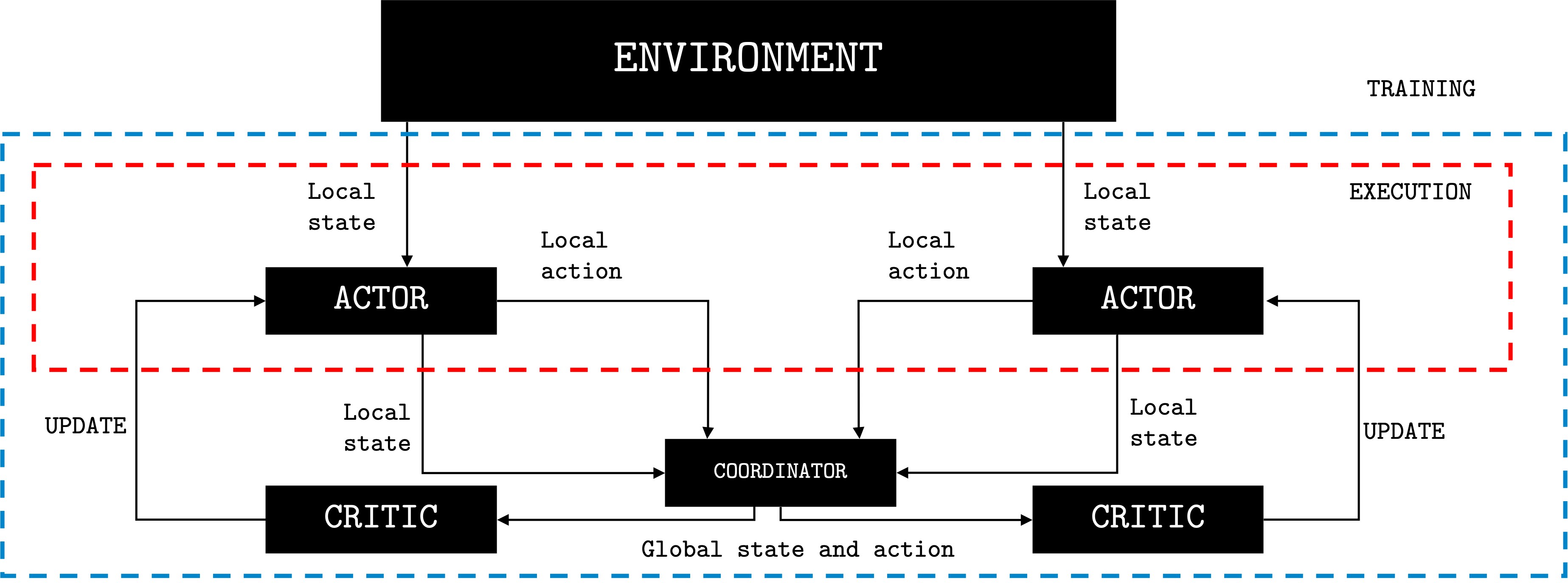
Figure 1: Schematic showcasing the Centralised Training Decentralised Execution framework

3 Methodology

In this section, we outline our approach for a graph-based multi-agent PPO algorithm. First, we discuss the integration of graph neural networks (GNNs) into our framework. Next, we illustrate how noise injection is utilized as a regularizer within the value function in our approach. Finally, we define the inventory management problem, outlining its key components and objectives.

3.1 P-GCN-MAPPO

In environments where the graph structure can be leveraged, Graph Neural Networks (GNNs) are commonly integrated into RL frameworks. GNNs were developed to efficiently leverage the structure and properties of graphs. GNNs operate on graph-structured data and are able to capture complex relationships and dependencies inherent in graphs. In this work, we use Graph Convolutional Networks (GCNs) combined with Multi-Agent Proximal Policy Optimization (MAPPO) and a Pooling strategy, hence P-GCN-MAPPO. In Section 4 we conduct computational experiments to analyze the different components of this methodology in an effort to distill their contribution to the overarching framework. GCNs update the representation of a node by aggregating and transforming the features of its neighbouring nodes and itself. This allows the model to capture and propagate local information, effectively learning patterns and dependencies from the graph structure of a supply chain. This ability to capture complex relationships is particularly beneficial for supply chain problems as understanding the intricate relationships between various entities can significantly optimize decision-making.

The adjacency matrix, $A\in\mathbb{R}^{N\times N}$, is a $N\times N$ matrix which is used to express the directed graph topology where $N$ is the number of nodes (or vertices) in the graph. In this matrix, $A_{ij}=1$ indicates that there is a connection between node $i$ and node $j$. Each node $i$ is associated with a node feature $x_{i}$ which encapsulates information specific to that node where $x_{i}\in\mathbb{R}^{D}$ where $D$ represents the dimensionality of the features vector. These individual node features collectively form the node feature matrix, $X\in\mathbb{R}^{N\times D}$. At each time step, the node feature matrix, $X$, captures the evolving state of the graph. Both $A$ and $X$ are fed into a graph convolution layer, allowing the model to capture relational information between nodes.

$$f(X,A)\coloneqq\sigma(D^{-\frac{1}{2}}(A+I)D^{-\frac{1}{2}}XW)$$ (7)

where $A\in\mathbb{R}^{N\times N}$ is the adjacency matrix, $I\in\mathbb{R}^{N\times N}$ is the identity matrix, $D\in\mathbb{R}^{N\times N}$ is the degree matrix of $A+I$, $X\in\mathbb{R}^{N\times D}$ is the node feature matrix, $W\in\mathbb{R}^{D\times W^{\prime}}$ is the layer’s weights where $W^{\prime}$ is the number of output features and $\sigma(.)$ is the activation function (e.g. ReLU). This results in an embedded vector for each node, $h_{i}\in\mathbb{R}^{W^{\prime}}$. In this work, three convolution layers are used where the embedded vector at each node, $h_{i}$, is the input of the next layer. This is described mathematically as:

$$H_{1} \coloneqq f_{W_{1}}(X,A)$$ (8)

$$H_{2} \coloneqq f_{W_{2}}(H_{1},A)$$ (9)

$$H_{3} \coloneqq f_{W_{3}}(H_{2},A)$$ (10)

where $H_{1}\in\mathbb{R}^{N\times W_{1}^{\prime}},H_{2}\in\mathbb{R}^{N\times W_{2}^{\prime}},H_{3}\in\mathbb{R}^{N\times W_{3}^{\prime}}$ are the embedded node matrices at layers 1,2 and 3 and $W_{1},W_{2},W_{3}$ are the weight matrices that parameterize each layer. The terms $W_{1}^{\prime},W_{2}^{\prime},W_{3}^{\prime}\in\mathbb{Z}^{+}$ are defined as positive integers representing the number of output features for each layer respectively. These values are hyperparameters that determine the dimensionality of the embedded vectors produced by each layer.

The resulting latent representations are then passed to our centralized value function $V_{\phi}(s)$, a fully connected network parameterized by $\phi$. This function assesses the value of actions, aiding in variance reduction of the policy $\pi_{\theta}$, another fully connected network parameterized by $\theta$, which maps states to actions. To train the policies, we employ Multi-Agent Proximal Policy Optimization (MAPPO). Mini-batches are sampled, and the objective is to minimize the loss function for each batch shown in Equation 2.2 which is used to update the parameters, $\theta$ and $\phi$.

However, as the number of agents increases, the dimensionality of the node feature changes. To address this, we propose integrating global mean pooling within our framework, ensuring dimensionality remains constant as the number of agents increases.

Pooling operators in graphs were inspired by pooling methods in Convolutional Neural Networks (CNNs). Therefore, instead of simply concatenating all the latent hidden representations and feeding them directly into our central value function, we enhance computational efficiency by employing the global mean pool operator. The global mean pooling operator aggregates information across all nodes in a graph by taking the average of the node features. The GNN outputs hidden feature matrix, $H\in\mathbb{R}^{N\times W_{3}^{\prime}}$ , can be denoted as $H=\{h_{1},h_{2},\dots,h_{N}\}$ where $N$ is the number of nodes and $h_{i}$ is the GNN output feature vector for node $i$. The global mean pooling operator computes the mean of each feature across all nodes.

$$\text{Global Mean Pool}(H)=\frac{1}{N}\sum_{i=1}^{N}h_{i}$$ (11)

This effectively reduces the input dimensions to our critic from $N\times W_{3}^{\prime}$ to $1\times W_{3}^{\prime}$. This is shown in Figure 2. While this dimensionality reduction improves computational efficiency, there’s a potential drawback: it may result in the loss of specific spatial information. However, since each individual actor still leverages local information for each node, the loss is confined to the critic. Moreover, the critic might not require the full level of spatial detail to assess the overall value of a state. The high-level features extracted through the global mean pooling mechanism might suffice. This idea has been explored in several studies such as Fujimoto et al. (2018) who highlights the critic’s focus on good enough value approximation for policy improvement, suggesting it may not need full state representation and Lyu et al. (2023) which proved that centralized critics may not be beneficial; particularly state-based critics can introduced unexpected bias. This aligns with the idea that the critic might not need a perfect representation but an accurate enough estimate for policy guidance. Finally, the global mean pooling mechanisms can also help mitigate the risk of overfitting, a common problem in RL where the model performs well on training data but poorly on unseen data. By reducing the number of features, the model focuses on the most relevant aspects, potentially leading to better generalization.

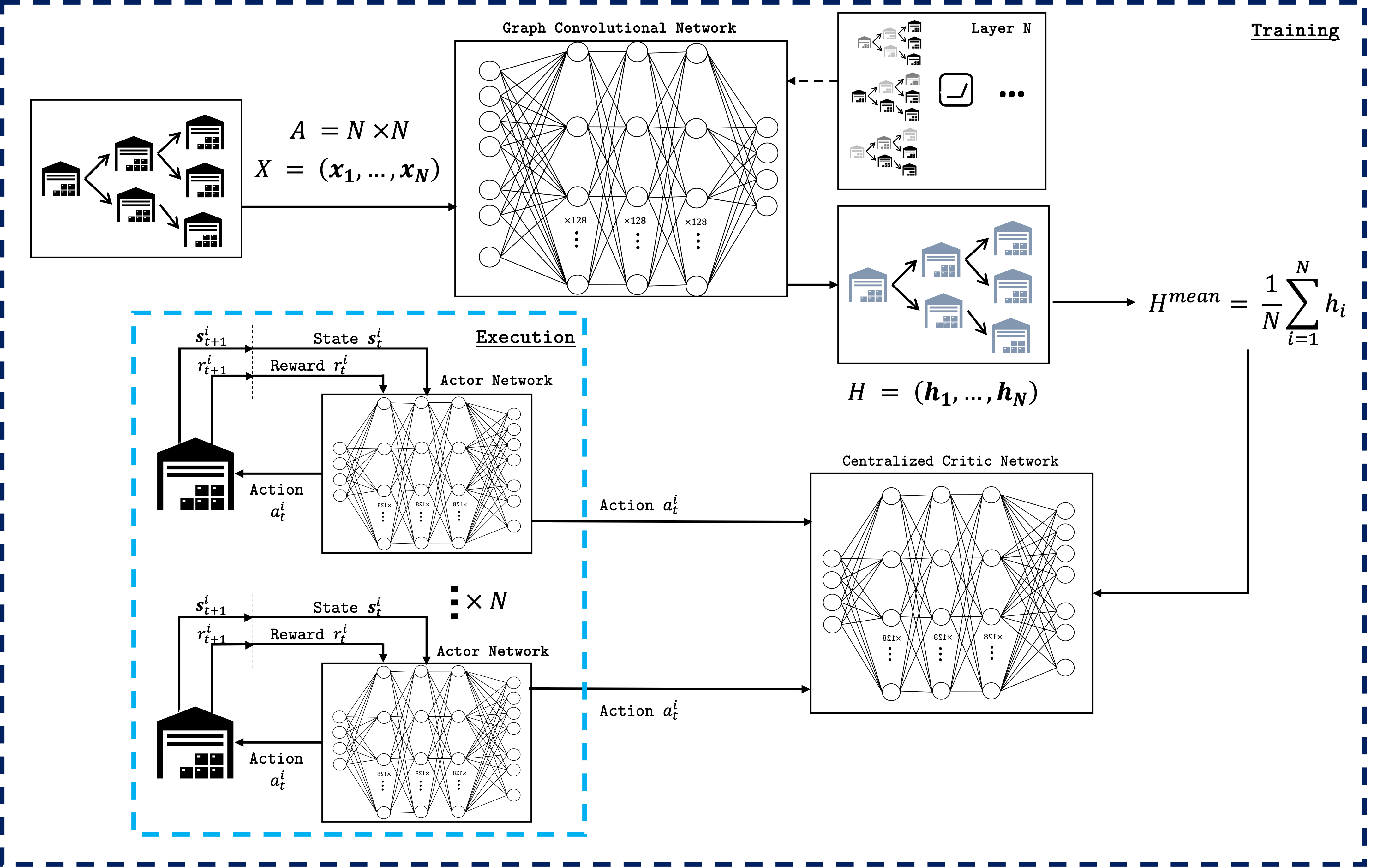
Figure 2: Methodology diagram outlining the P-GCN-MAPPO framework, illustrating the key components and processes involved.

3.2 Noisy P-GCN-MAPPO

The problem of policy over-fitting occurs as the estimated advantage is the same for all agents leading to the lack of credit assignment. Theoretically, this can be solved by ensuring the shared advantage value does not affect other agents by decomposing the centralized advantage value for each agent. However, given the nature of multi-agent systems, this is impractical. Therefore, noise can be introduced as a regularize to reduce bias in advantage values. Noise has been extensively studied and used in several forms across different components of reinforcement learning, including action space exploration and observation perturbation. In this work, we focus on introducing noise specifically in the value function which then propagates to the estimation of advantage values as shown in Figure 3. This approach offers several potential benefits and implications:

1. Reduces Overfitting and Biases. Introduction of noise reduces over-fitting and biases in advantage value estimations. The introduction of randomness into the value function, means any patterns or biases that may arise from the agent’s limited experience or observations are disrupted.

2. Exploration Enhancement. The introduction of noise in the value function promotes exploration by injecting randomness into the agent’s value estimates.

We sample a Gaussian noise,

$$\epsilon_{n}\sim\mathcal{N}(0,\sigma^{2})$$ (12)

where $\sigma^{2}$ is the variance (intensity) of the noise added to the samples. The value of $\sigma$ is a hyperparameter controlling the noise level, we analyse the effect of this hyperparameter in Section 4.2. The global state, $s$, is then inputted into the centralized value network $V_{\phi}$ to which the sampled noise, $\epsilon_{n}$, is added.

$$V_{\phi}(s)\leftarrow V_{\phi}(s)+\epsilon_{n}$$ (13)

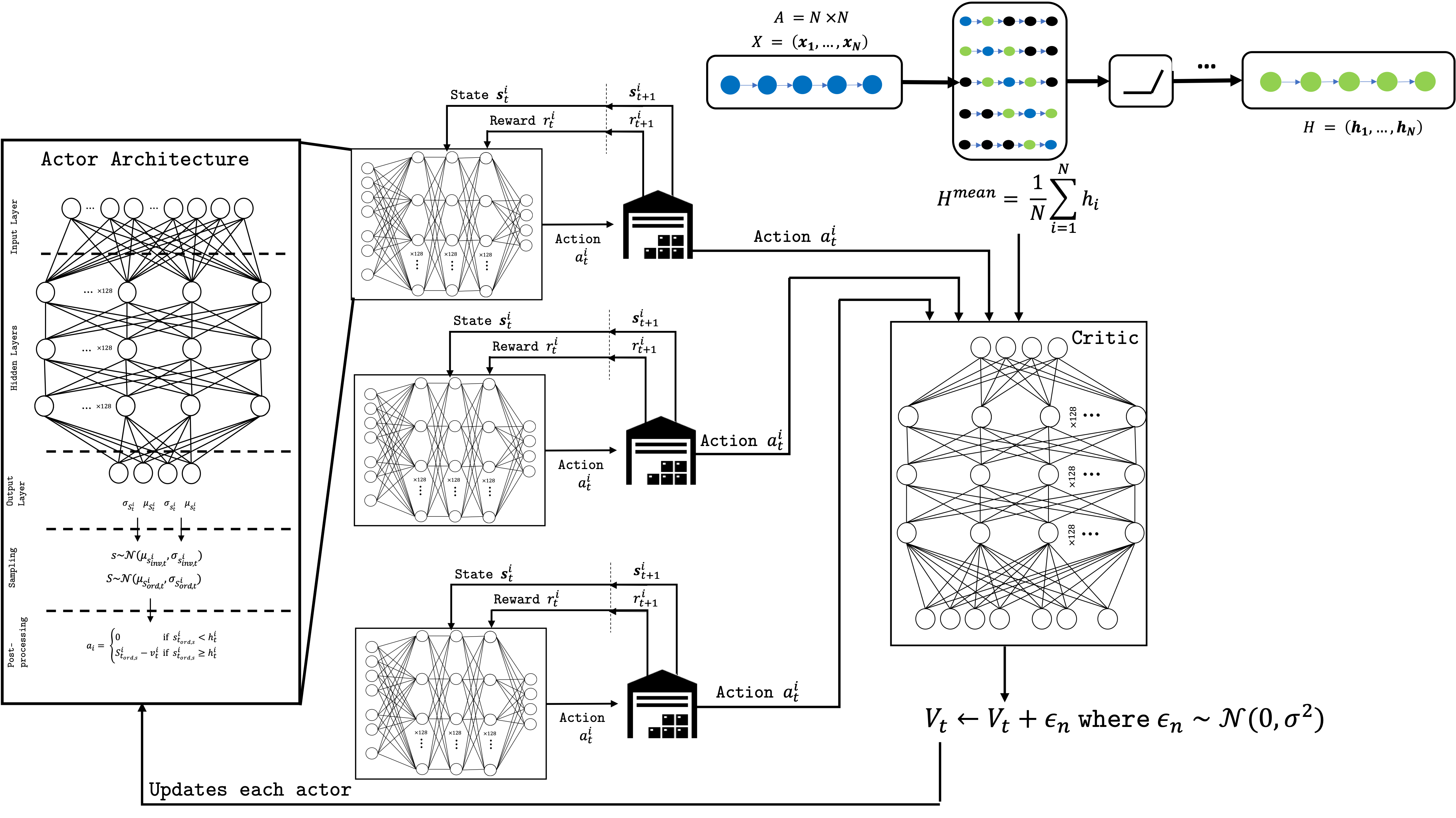
(a) Overview of the training phase, illustrating the collaboration between the actor, critic, and graph convolutional neural networks for multiple actors.

(b) Illustration of value function noise injection within the actor-critic framework for a single actor.

Figure 3: Visual representations of the training processes: (a) the interaction among multiple actors during training, and (b) the role of noise injection in enhancing the learning dynamics shown with a single actor.

The addition of the random noise disturbs the value function uniformly for all agents which is propagated to the advantage function. Uniform noise injection introduces variability into the advantage values, promoting exploration and adaptability across the entire agent population. This in turn provides benefits such as preventing overfitting caused by sampled advantage values with deviations and environmental non-stationarity. However, it’s important to note that this approach may sacrifice the potential for agents to fully exploit their individual characteristics and preferences, which tailored noise could accommodate.

An additional advantage of Proximal Policy Optimization (PPO), is the inherent clipping mechanism of the algorithm which helps mitigate potential instability caused by the noise. The clipping ensures policy updates remain close to the previous policy allowing for exploration benefits introduced through value function noise injection without compromising training stability.

3.3 Problem Statement

The cooperative nature of the MARL scenario that we consider means agents coordinate towards a common goal, receiving a shared reward. This sequential decision making problem is modelled as a Decentralized Partially Observable Markov Decision Process (Dec-POMDP), which can be defined as a tuple $\left\langle\mathcal{S},\mathbf{A},\mathcal{T},\mathcal{R},\Omega,\mathcal{O},\gamma\right\rangle.$ $\mathcal{S}$ is the set of all valid states, $\mathbf{A}\coloneqq\mathbf{A}^{1}\times\dots\times\mathbf{A}^{N}$ is the joint action space where $\mathbf{A}^{i}$ is the set of actions available for each agent $i$, $\Omega\coloneqq\Omega^{1}\times\dots\times\Omega^{N}$ is the joint observation space and $N$ denotes the number of agents. At each time step, each agent $i$ executes action ${a}^{i}\in\mathcal{A}^{i}\subseteq\mathbb{R}^{n_{a}}$ with a joint action $\textbf{a}=\left\langle a^{1},\dots,a^{N}\right\rangle$ and transitions from state $s\ \in\mathcal{S}\subseteq\mathbb{R}^{n_{s}}$ to $s^{\prime}\in\mathcal{S}\subseteq\mathbb{R}^{n_{s}}$ with state transition probability $P(s^{\prime}|s,\textbf{a})=\mathcal{T}(s,\textbf{a},s^{\prime})$. Each agent $i$ receives observation $o^{i}\in\Omega^{i}\subseteq\mathbb{R}^{n_{o^{i}}}$ determined by $\mathcal{O}(s^{\prime},i)$ which maps the new state $s^{\prime}\in\mathcal{S}$ to an observation $o^{i}\in\Omega^{i}$ for each agent $i$. In other words, the observation function $\mathcal{O}:\mathcal{S}\times\{1,\dots,N\}\rightarrow\Omega$ provides each agent $i$ with a local observation $o^{i}$ based on the next state $s^{\prime,i}$. The joint observation can be defined as $\textbf{o}=\left\langle o^{1},\cdots,o^{N}\right\rangle$ and each agent shares the same reward function $\mathcal{R}(s,\textbf{a})\in\mathbb{R}$. Each agent has policy $\pi^{i}$ and the joint policy is denoted as $\mathbf{\pi}=\ \left\langle\pi^{1},\cdots,\ \pi^{N}\right\rangle$. The optimal joint policy is found through maximising the joint expected reward $\mathbb{E}\left[\sum_{t=0}^{t=T}\gamma^{t}r_{t}\right]$ where $r_{t}\ =\ \mathcal{R}\left(s_{t},\ a_{t}\right)\ \in\mathbb{R}$ at each time step $t$ where $T$ is the time horizon and the discount factor $\gamma\in\left[0,1\right]$.

To find the optimal inventory policy in the inventory management problem, we propose a mathematical formulation of the supply chain dynamics as an optimization problem, characterized by each time period $t$, over a fixed horizon of $T$ time periods. The variables are defined in Table 1.

Table 1: Variables and Parameters for the Inventory Management Problem

Symbol	Description
$i$	Node $i\in N$ where $N$ is the total number of nodes
$g\in\mathbb{R}^{n_{i_{d}}}$	Amount of goods shipped from node $i$ to downstream nodes
$o_{r}\in\mathbb{R}$	Replenishment order
$d\in\mathbb{R}$	Demand from downstream nodes
$v\in\mathbb{R}$	On-hand inventory
$b\in\mathbb{R}$	Backlog
$q\in\mathbb{R}$	Acquisition or incoming goods
$v_{0}\in\mathbb{R}$	On-hand inventory at the start of each period
$b_{0}\in\mathbb{R}$	Backlog at the start of each period
$P\in\mathbb{R}^{n_{N}}$	Price of goods sold
$C\in\mathbb{R}^{n_{N}}$	Order replenishment costs
$V\in\mathbb{R}^{n_{N}}$	Storage costs
$B\in\mathbb{R}^{n_{N}}$	Backlog costs
$V_{\max}\in\mathbb{R}^{n_{N}}$	Maximum limits on node storage
$O_{r,\max}\in\mathbb{R}^{n_{N}}$	Maximum limits on replenishment order quantities
$i_{u}\in\mathbb{R}$	Upstream node of $i$
$i_{d}\in\mathbb{R}$	Downstream node of $i$
$b^{i}=\sum_{j\in\mathcal{D}_{i}}b^{i_{d}}$	Total backlog of node $i$ from downstream nodes
$g^{i}=\sum_{j\in\mathcal{D}_{i}}g^{i_{d}}$	Total shipment of node $i$ to downstream nodes
$\mathcal{D}_{i}$	Set of direct downstream nodes $j$ of node $i$ where $j\in\mathcal{D}_{i}$
$\mathcal{C}$	Set of nodes with customer demand
$c$	Customer demand

Equation (LABEL:eqn:_optimisation) is the objective function that maximizes total profit across the supply chain system. The system is treated as a collaborative framework, where all agents in the network share a common objective function, reward $r_{t}$. Equation (LABEL:eqn:_inventory) and (LABEL:eqn:_backlog) show how the inventory and backlog are updated over time. Equations (LABEL:eqn:_sales_constraint_2) and (LABEL:eqn:_sales_constraint_1) restrict the quantity of goods a node can ship downstream, ensuring it does not exceed the on-hand inventory or the downstream demand and backlog. Equation (LABEL:eqn:_acquisition) and LABEL:eqn:_factory capture the lead time of a shipment, indicating that goods shipped to node $i$ will take $\tau^{i}$ periods to reach the downstream stage. The amount of inventory hold or ordered is also constrained to a maximum value through Equations LABEL:eqn:_limits. The interaction of the different flows between two nodes can also be seen in Figure 4.

$$\begin{split}\scriptscriptstyle&\max\sum_{i=1}^{N}\sum_{t=1}^{T}P^{i}g^{i}[t]-C^{i}o_{r}^{i}[t]-V^{i}v^{i}[t]-B^{i}b^{i}[t]\,,\end{split}$$ (14)

$$\begin{split}&\text{subject to}\end{split}$$

$$\begin{split}&v^{i}[t]=v_{0}^{i}[t]-g^{i}[t]+q^{i}[t]\,,\quad\forall i,\forall t,\end{split}$$ (15)

$$\begin{split}&b^{i_{d}}[t]=b_{0}^{i_{d}}[t]-g^{i_{d}}[t]+d^{i_{d}}[t],\quad\forall i,\forall d\in\mathcal{D}_{i}\,,\end{split}$$ (16)

$$\begin{split}&g^{i_{d}}[t]\leq b_{0}^{i_{d}}[t]+d^{i_{d}}[t]\,,\quad\forall i,\forall t,\forall d\in\mathcal{D}_{i}\end{split}$$ (17)

$$\begin{split}&g^{i}[t]\leq v_{0}^{i}[t]+q^{i}[t],\quad\forall i,\forall t,\end{split}$$ (18)

$$\begin{split}&q^{i}[t]=g^{i_{u}}[t-\tau^{i}],\quad\forall i\neq 1\,,t\geq\tau^{i}\end{split}$$ (19)

$$\begin{split}&q^{1}[t]=o_{r}^{1}[t-\tau^{1}],\quad t\geq\tau^{1}\end{split}$$ (20)

$$\begin{split}&d^{i_{d}}=o_{r}^{d},\quad\forall i,\forall d\in\mathcal{D}_{i}\,,\end{split}$$ (21)

$$\begin{split}&\text{with}\end{split}$$

$$\begin{split}&d^{i}[t]=c^{i}[t],\quad\forall i\in\mathcal{C},\forall t\end{split}$$ (22)

$$\begin{split}&o_{r}^{i}[t]\leq O_{r,\max}^{i}\,,v^{i}[t]\leq V_{\max}^{i}\,,\quad\forall i,\forall t,\end{split}$$ (23)

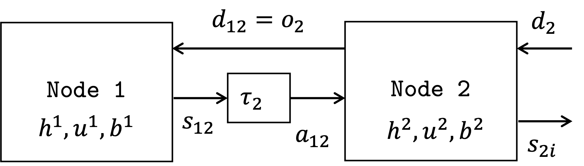
Figure 4: Schematic showing the inventory flow between two nodes in an inventory management system

The demand and lead time are uncertain, modelled as a Poisson random variable with parameter $\lambda$ and $\mu$ respectively. Therefore, the probability of $k$ demands in a time period $t$ is given by:

$$P(D=k)=\frac{(\lambda t)^{k}\exp^{-kt}}{k!}$$ (24)

Moreover, inventory management system can be modelled as a graph $G=(W,E)$ where $W$ represents different entities in the supply chain (e.g. factories, manufacturers, warehouses), $E$ denotes the relationship between these entities, and each node $i\in W$ corresponds to an agent responsible for managing inventory at that entity’s location. Each node $i$ has a node feature $x^{i}\in X$, representing the observation space $o^{i}$ for each agent. The observation set for each agent $i$ is $o^{i}=[v,b,p,d^{-1},\dots,d^{-M},o_{r}^{-1},\dots,o_{r}^{-M}]$ where $o^{i}\ \in\Omega^{i}$. In the observation set, a new variable is introduced, $p$, which is the pipeline inventory equal to the sum of order replenishment that has not yet arrived at the node from other upstream nodes. To mitigate the problem of partial observability, we include demand history and order history up to $M$ time-steps in the past where $M$ is a hyperparameter. While we chose not to incorporate Recurrent Neural Networks (RNNs) in this work, which could effectively handle sequential data and temporal dependencies, we acknowledge their potential as an alternative approach. Our decision to include a fixed window of past observations instead allows for a simpler implementation while still capturing relevant historical context.

However, this inclusion of historical data introduces a violation of the Markov property, which states that the future state of the system only depends on the current state and not on the sequence of events that preceded it. However, real-world decision-making processes rarely exhibit perfect Markovian behavior. Therefore, including historical data is a well-established approach to augment the observation space in partially observable environments Liu et al. (2022a); Mousa et al. (2023); Uehara et al. (2022).

The neighbourhood of a node $i$, denoted by $M(i)$ is defined as the set of neighbouring nodes $j$ connected to node $i$ via edges in $E$. Mathematically, this can be represented as $M(i)=\{j|(i,j)\in E\}$. For each node $i$, the features of its neighbours $j$ are represented as $x_{j}^{i}$, capturing the relevant observations of the neighbouring agents.

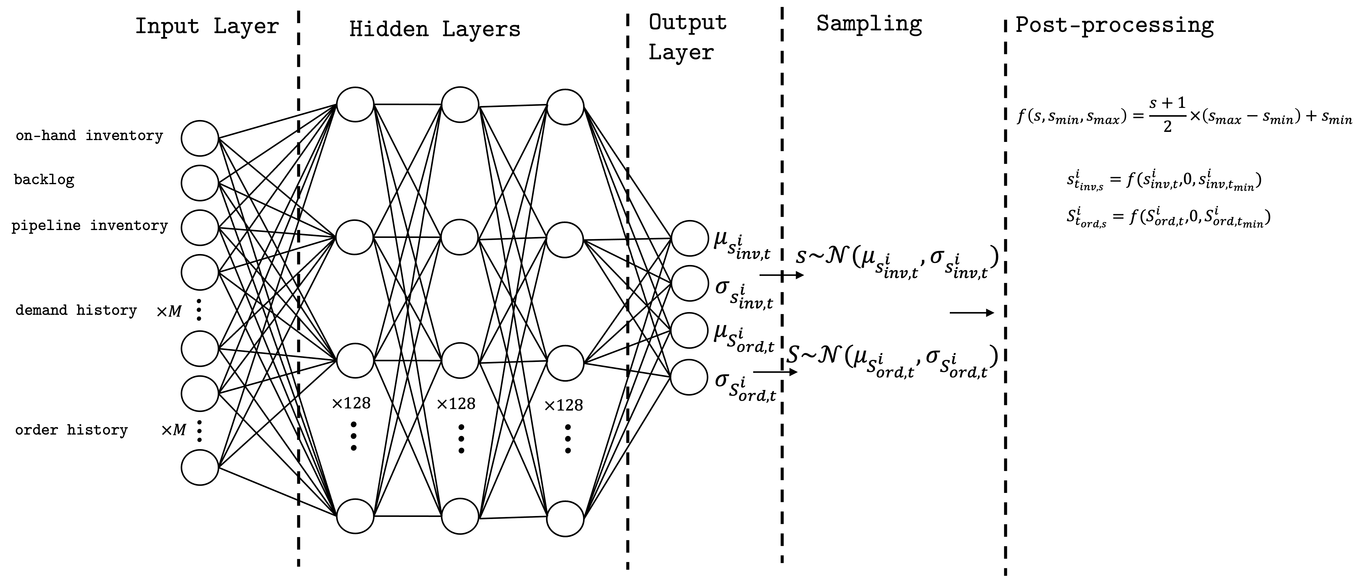
Figure 5: Neural network architecture for actor, illustrating sampling from a Gaussian distribution, followed by a post-processing step, leveraging an inventory heuristic policy to generate actions in a continuous action space.

Moreover, the action space is traditionally modelled as the order replenishment quantity, $o$. However, in this paper we parameterize a heuristic inventory policy such that for each agent $i$, at each time step $t$, the policy outputs a mean and standard deviation for both $s_{\text{inv},t}^{i}$ and $S_{\text{ord},t}^{i}$. Therefore, $\pi_{i}(o^{i})=(\mu_{s_{\text{inv},t}^{i}},\sigma_{s_{\text{inv},t}^{i}},\mu_{S_{\text{ord},t}^{i}},\sigma_{S_{\text{order},t}^{i}})$ and the heuristic inventory parameters are sampled from a Gaussian distribution, $s_{\text{inv},t}^{i}\sim\mathcal{N}(\mu_{s_{\text{inv},t}^{i}},\sigma_{s_{\text{inv},t}^{i}}^{2})$, $S_{\text{ord},t}^{i}\sim\mathcal{N}(\mu_{S_{\text{ord},t}^{i}},\sigma_{S_{\text{ord},t}^{i}}^{2})$. A min-max post processing step is then used to scale the values to a suitable range denoted by a subscript $s$, leading to $(s_{t_{\text{inv,s}}}^{i},S_{t_{\text{ord,s}}}^{i})$ where $s_{t_{\text{inv,s}}}^{i}$ is the reorder point and $S_{t_{\text{ord,s}}}^{i}$ is the order-up-to-level. When the inventory reaches a level of $s_{t_{\text{inv,s}}}^{i}$, an inventory order is placed where $o_{r,t}^{i}=S_{t_{\text{ord,s}}}^{i}-v_{t}^{i}$. The neural network architecture for each actor, including the post-processing step that results in the order replenishment quantity, is illustrated in Figure 5.

Moreover, in inventory management, optimal order quantity policies such as $(s_{t_{\text{inv,s}}}^{i},S_{t_{\text{ord,s}}}^{i})$ are often characterized by discrete functions as they show abrupt changes in order quantity at specific inventory levels Dehaybe et al. (2024). This poses a challenge for neural networks, which are inherently continuous function approximators as directly approximating such discrete policies can lead to instability and poor performance in neural network-based models. To address this, in this paper, the actor network outputs a normal distribution (Gaussian) over the $(s_{t_{\text{inv}}}^{i},S_{t_{\text{ord}}}^{i})$ parameters. A key note is that this approach does not limit the network’s ability to learn the optimal policy as it simply expresses the policy in a way that may be easier to learn. Moreover, unlike traditional heuristic methods where the policy is not conditioned on the state of the system, an RL approach means the heuristic $(s_{t_{\text{inv,s}}}^{i},S_{t_{\text{ord,s}}}^{i})$ policy is conditioned on the state of the system such as on-hand, pipeline inventory and backlog. This enables the agent to dynamically adjust the reorder point and order-up-to level based on the current inventory situation, potentially leading to optimal and flexible decision-making.

Finally, while the actual order replenishment quantities in our environment are discrete, we model the action space for each agent as continuous within the range of $\left[-1,1\right]$. This approach facilitates scalability to problems with a wider range of possible order sizes. To bridge the gap between the continuous action space and the discrete nature of order quantities, we employ a post-processing step using min-max scaling. During this step, the agent’s chosen action is scaled to the appropriate range for the order replenishment variable and then rounded to the nearest integer value.

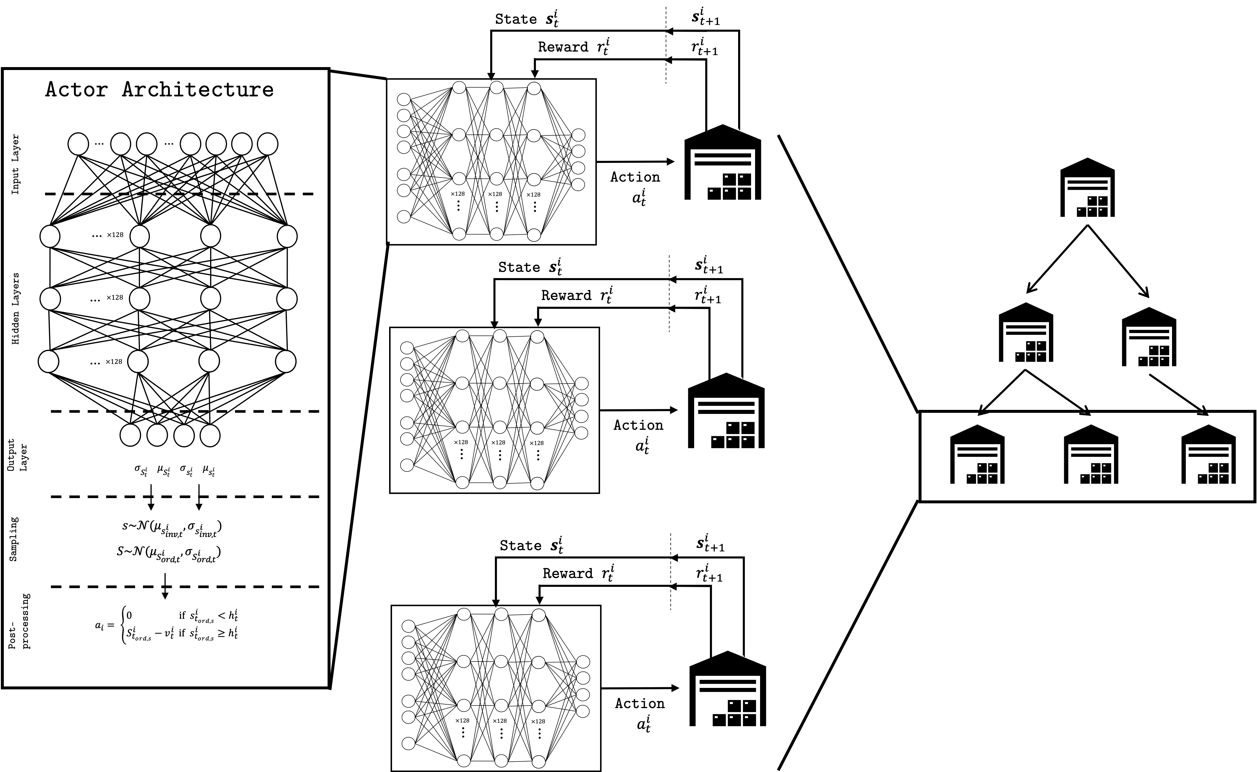
Figure 6: Schematic illustrating the execution of the trained policies simultaneously alongside heuristic inventory control policies.

4 Results and Discussion

In this section four case studies of different inventory management configurations are used to illustrate the effectiveness of our proposed methodology as shown in Figure 7. We compare our proposed methodology (Noisy P-GCN-MAPPO and P-GCN-MAPPO) against other MARL methods including: IPPO, MAPPO, and Graph-based-MAPPO(G-MAPPO). This allows us to compare against state-of-the-art as well as analyse the contribution of the different components of our method. One of the key differences between the methods is the varying levels of information input to the value function which can be illustrated qualitatively in Figure 8. This is further benchmarked against single agent RL (PPO specifically) and a heuristic (s,S) policy. In the later, a static heuristic policy is found for each node in the network, where optimal parameters are found using a derivative-free method, implemented using SciPy Virtanen et al. (2020) with a multi-start approach combined with local search.

All variant MARL algorithms are implemented in the Ray RLLib framework Liang et al. (2018), and all the hyperparameters are kept the same as the baseline algorithms to ensure fairness.

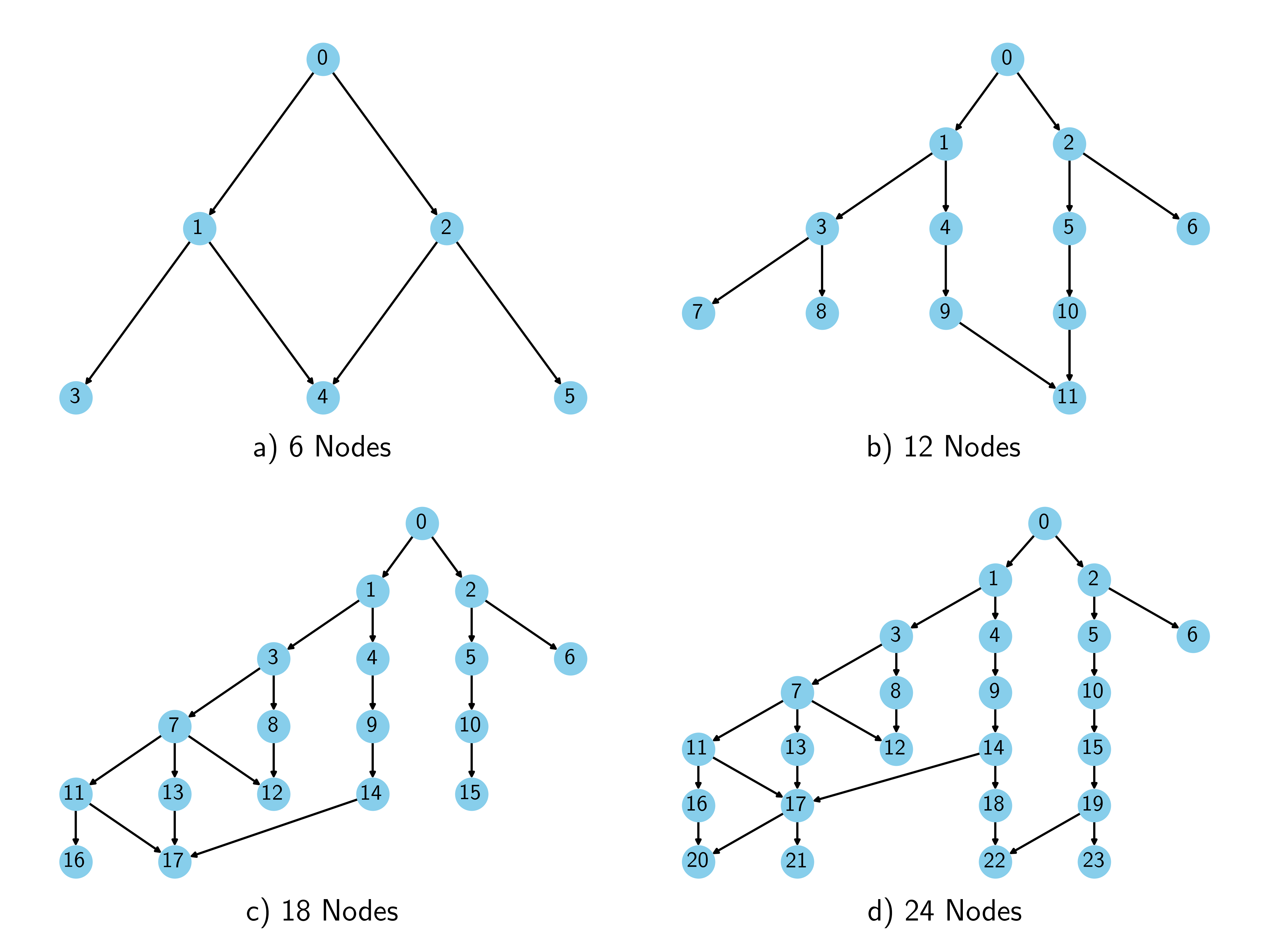
Figure 7: Different supply chain configuration case studies with varying number of nodes

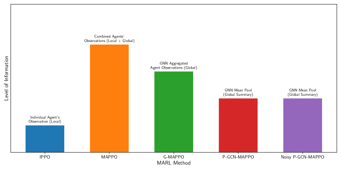
Figure 8: Qualitative representation of varying levels of information input to the value function. The different levels illustrate how changes in observability can affect performance.

4.1 Execution

To evaluate the performance and robustness of our proposed methodology, we considered different scenarios involving a varying number of agents: 6, 12, 18, and 24 agents. Each scenario represents a different level of complexity and coordination required among the agents. In order to assess our methodology, we observe the performance of the trained policies on 20 simulated test episodes with 50 time-steps each. Both the lead time and demand uncertainty remained constant throughout the test episodes and each methodology. All methodologies follow the CTDE framework where agents only require local information at execution. The execution of the MARL algorithms in these scenarios was assessed through performance metrics including cumulative reward, backlog and inventory levels.

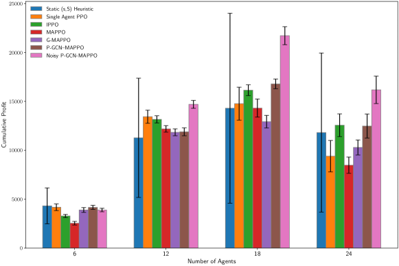
Figure 9: Cumulative Profit (with Standard Deviation) for the different methodologies across the four different supply chain configurations

Firstly, the bar graph shown in Figure 9 compares the cumulative profit for the different methodologies in the different supply chain network configurations. Notably, the proposed methodology, Noisy P-GCN-MAPPO, has on par performance or outperforms the other methodologies. This advantage becomes increasingly pronounced as the number of agents rises. This trend suggests that Noisy P-GCN-MAPPO may be particularly effective in large-scale, multi-agent inventory control scenarios. The decrease in cumulative profit from the 18 agent to 24 agent configuration can be attributed to differences in number of retailers present and the specific environment configuration chosen. Figure 9 also shows that while the static $(s_{t_{\text{inv,s}}}^{i},S_{t_{\text{ord,s}}}^{i})$ policy achieves similar cumulative profit performance to Noisy P-GCN-MAPPO, it exhibits a significantly higher standard deviation. This variability suggests that the static heuristic is less stable, potentially hindering its robustness in situations with unexpected changes to the environment.

This distinction is crucial in real-world applications, where supply chain networks and other multi-agent systems inevitably encounter unexpected events. RL’s ability to maintain good performance in uncertain environments is one of the key advantages compared to traditional methods. Therefore, the results highlight the strength of RL methods, particularly Noisy P-GCN-MAPPO, as its lower standard deviation suggests greater potential for robustness and adaptability in uncertain environments.

Figure 10(a), illustrates the median backlog for different algorithms. The static $(s_{t_{\text{inv,s}}}^{i},S_{t_{\text{ord,s}}}^{i})$ heuristic exhibits a significant increase in backlog as the number of agents rises. This trend suggests potential difficulties in handling the growing complexity of the environment with more agents (e.g., increased number of interactions, coordination challenges). The static nature of the inventory policy in the static $(s_{t_{\text{inv,s}}}^{i},S_{t_{\text{ord,s}}}^{i})$ heuristic might also contribute, as it cannot adapt to changing environmental conditions. In contrast, our proposed methodology addresses this limitation by redefining the action space to parametrize a heuristic policy. This allows our policy to be more adaptive and adjust its behavior based on the current state of the environment, potentially leading to better handling of increased complexity and reducing the backlog. However, from Figure 10(b), only minimal differences were present in the final on-hand inventory across methodologies.

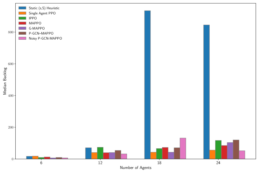
(a) Backlog

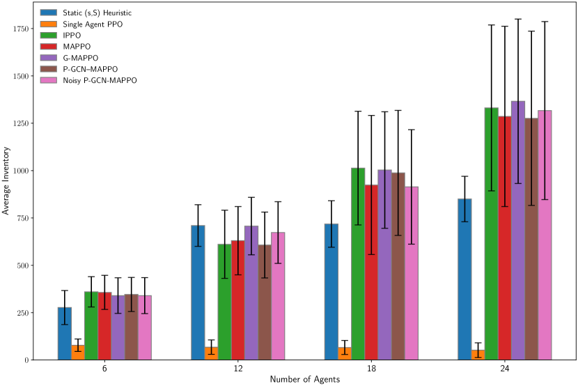
(b) Inventory

Figure 10: Median metric along with standard deviations for the different methodologies and configurations

Our methodology is also compared with other MARL methods. The notable difference between them is the information available to the critic. One key challenge in MARL is balancing access to global information (mitigating non-stationarity) with scalability limitations of naively combining all agent states. Our proposed methodologies, P-G-MAPPO and Noisy P-GCN-MAPPO, address this by leveraging graph-based approaches and the inherent structural properties of the problem. This allows agents to exploit both local and global information effectively.

Figure 11 shows how IPPO consistently outperforms MAPPO, and this performance gap widens with a greater number of agents. This motivated the development of smarter methods of information aggregation, by leveraging graph-based approaches, where information can be harnessed whilst not suffering from performance shortcomings. This highlights the need for smarter information aggregation. G-MAPPO, P-GCN-MAPPO and Noisy P-GCN-MAPPO incorporate Graph Neural Networks (GNNs) to enable communication and information sharing while maintaining focus on local details.

However, from Figure 11, the G-MAPPO method does not always outperform MAPPO and IPPO methods. This may occur for similar reasons why IPPO outperforms MAPPO. Too much information may be captured leading to the policies overfitting. Therefore, P-GCN-MAPPO outperforms G-MAPPO, MAPPO and IPPO in all 4 case studies. This occurs as the integration of a pooling mechanism, can help aggregate information from different parts of the graph, reducing the dimensionality of the data acting as a regularizer and potentially reducing overfitting. The message passing inherent in graph neural networks allows for agents to inherently communicate with each other whilst the pooling mechanism prevents overfitting of the policies. Despite losing local information in the critic, the global mean pooling mechanism allows for global information to be captured in the central critic that helps reduce the variance in the individual actors that are trained with local information.

Our final proposed methodology hypothesizes that the addition of noise into the value function, propagates variability into the advantage function potentially reducing overfitting. The execution curves shown in Figure 11 show the impact of adding noise to the value function on our methodology’s performance. The results show that with a small number of agents (6 agents), adding noise into the value function does not outperform P-GCN-MAPPO compared to when the number of agents is larger (24 agents). When the number of agents is 6, the overall state space is smaller compared to a large agent system. Therefore, the addition of noise will just add unnecessary randomness which could disrupt the learning process as opposed to benefit the training of the policies. However, as the number of agents increases, it becomes harder for traditional MARL algorithms to explore the entire space efficiently. Therefore, large agent systems are more prone to getting stuck in local optima. The addition of noise to the value function encourages the agents to explore a wider range of actions, leading towards better solutions. The addition of noise can also be seen as regularization, where the policies become more robust to the complex environment.

(a) 6 nodes

(b) 12 nodes

(c) 18 nodes

(d) 24 nodes

Figure 11: Execution curves for the 4 different supply chain configurations.

Moreover, it is useful to compare the change in entropy during the training phase for each of the different methods. In the context of MARL, entropy quantifies the uncertainty or randomness in the policy’s action distribution (Sutton, 2018). During the training process, as the agents learn, the entropy in the policy distribution decreases as the agents learn better policies. Figure 12 shows that the rate of entropy decrease differs between the different methods. The addition of noise to the value function introduces controlled variability which propagates into the advantage estimates. This helps maintain a higher entropy for a longer period during training which is desirable as high entropy promotes exploration. During MARL training, agents need to balance exploring new actions and exploiting known good actions. By exploring a wider range of actions (due to high entropy), agents are more likely to discover better strategies and avoid getting stuck in sub-optimal solutions. This can be especially important in complex environments where the best course of action depends on what other agents are doing. Figure 12 shows that Noisy P-GCN-MAPPO, maintains a higher entropy throughout training, promoting exploration and reducing policy overfitting leading to superior performance.

Figure 12: Figure shows the change in entropy during the training process for the different methods in the 18 agent configuration

4.2 Sensitivity to Gaussian Noise

In addition to acting as a regularizer, the incorporation of Gaussian Noise into the value function of MARL algorithms facilitates a balance between effective exploration and exploitation, a well known phenomena in the field of reinforcement learning. The following section will explore this sensitivity to noise intensity, examining how both insufficient and excessive noise can negatively impact the performance of MARL agents.

The standard deviation values were changed from 0.0, 0.1, 0.2, 0.5, 1.0 and 2.0. Figure 13(a) shows the cumulative profit of the agents at execution of the trained policies. The performance increases up to a standard deviation of 0.5. After which, when the noise intensity increases, the overall performance decreases. This occurs as when the standard deviation of the Gaussian distribution is small, there’s insufficient noise, leading to a lack of regularization. This can result in overfitting, limited exploration, and a tendency to settle into local optima. This is particularly detrimental in scenarios with large state spaces, where effective exploration becomes crucial for agents to learn optimal policies. Conversely, when the standard deviation is 1.0 and 2.0 the overall performance becomes worse as seen in Figure 13(a). This occurs when the noise intensity is too high, excessive noise can introduce significant randomness, increasing the variance in the value function which disrupts the learning process which may hinder convergence.

Moreover, the entropy during training is compared in Figure 13(b) for the noise value that performed best [0.5], the noise value that performed worst [0.1] and the base case scenario [0.0]. The results show that using a noise level with standard deviation = 0.5 leads to a higher final entropy compared to the scenario with no noise (standard deviation = 0.0). However, throughout the training process, when the noise intensity is high (standard deviation = 2.0), the entropy remains higher, emphasizing that this noise has introduced significant randomness leading to suboptimal policies.

Therefore, finding a level of noise becomes important, as it can act as a regularizer, promoting exploration in complex environments while maintaining a level of stability that allows for effective learning. This delicate balance is particularly important in settings with a large number of agents, where the vast state space and intricate interactions require a measured approach to exploration via noise injection.

(a) Execution curves at different levels of noise

(b) Change in entropy from 3 different noise levels

Figure 13: Sensitivity of noise intensity was performed for the 18 agent configuration

4.3 Scalability

This section explores the scalability of the different methodologies examined in this paper.

Firstly, Figure 14, depicts the training curves for 60 iterations across the four different configurations consisting of 6, 12, 18 and 24 agents. As the number of agents increases, it can be seen that it takes slightly longer to reach convergence due to the increased complexity of the learning process. However, the figure also shows that the policies for all configurations converge within the 60 iterations. Figure 14 also shows that despite the injection of noise in the value function, this does not cause instability in training due to the inherent clipping mechanism in PPO which ensures the policy update stays within a certain limit, maintaining stability.

(a) 6 agents

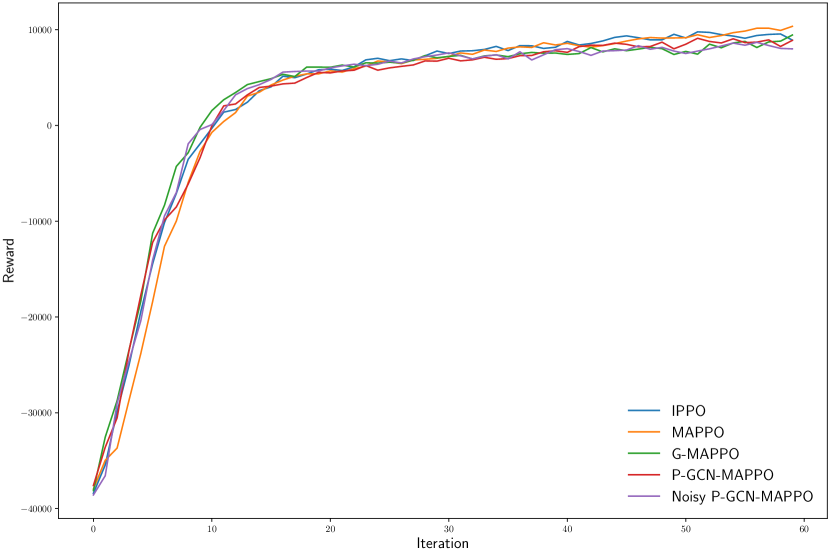
(b) 12 agents

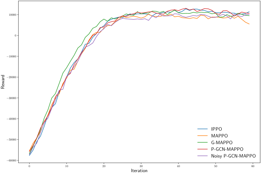
(c) 18 agents

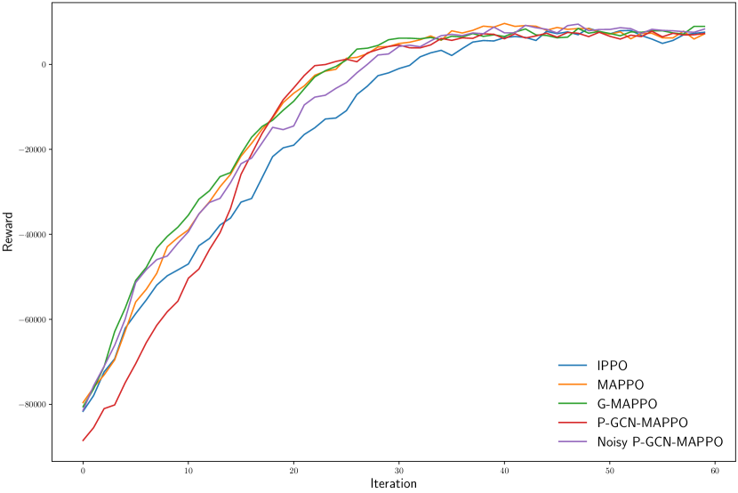
(d) 24 agents

Figure 14: Figure shows the training curves for 60 iterations for the 4 different configurations

Moreover, Figure 15, compares the mean training time per iteration in seconds both in terms of methodologies and number of agents. As expected, as the number of agents increases, the training time per iteration increases due to the increased complexity of the learning process. The methodologies leveraging the graph structure also have a higher mean training time per iteration because they require complex message passing between agents in the graph. G-MAPPO, P-GCN-MAPPO, Noisy P-GCN-MAPPO utilize a GNN which requires training alongside the policies. Therefore, extracting and processing information from the graph structure itself adds computational overhead compared to simpler MARL approaches. As the number of agents increases, the training time per iteration increases at a faster rate for the methodologies using GNNs as the communication and information processing becomes increasingly complex as the number of agents and complexity of the structure increases. However, Figure 15 shows that methods with an integrated pooling mechanism have faster training times than those without one. This further emphasises the scalability advantage of integrating a pooling mechanism compared to a standard GNN architecture in a MARL framework. The integration of the pooling mechanism reduces the dimensionality of the input to the central critic, reducing the computational overhead which leads to faster training times. Therefore, as opposed to naïvely concatenating information, MARL frameworks that employ smart information aggregation techniques can offer several advantages: reduced computational complexity, improved scalability and potential for improved performance by efficient aggregation that can lead to better representation of the global state.

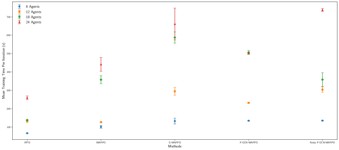
Figure 15: Box plot showing the mean training time per iteration (s) along with the associated standard deviation. Note: a z-test score was performed to remove anomalies of values which were 2 standard deviations greater than the mean value.

5 Conclusions and Future Work

In this work, we propose a new methodology that develops a decentralized decision-making framework for inventory management. Our framework leverages the inherent graph structure and reduces policy overfitting by Gaussian noise injection in the value function. Our approach also offers several advantages that enhance the efficiency and effectiveness of inventory systems.

Firstly, our approach redefines the action space by parameterizing a known heuristic inventory control policy which is often discontinuous in nature. Unlike traditional heuristic methods where the policy is not conditioned on the state of the system, leveraging an RL approach means the heuristic is conditioned on the state of the system. This not only allows for a more flexible decision-making framework but ensures earlier adoption of novel optimization techniques in industry due to its interpretability.

Secondly, our methodology overcomes information sharing constraints at an online level but trains the control policies in a collaborative framework. This ensures effective coordination and communication is present within the different entities of the inventory management system. The communication between entities is further enhanced by leveraging the inherent graph structure of a supply chain. This also shifts the costs from online to offline, resulting in a more efficient stochastic optimal control policy. The methodology results in a closed-loop solution rather than an open-loop optimization problem which enhances fast, real-time decision-making capabilities.

Overall we show that the addition of noise, particularly in a system with a larger number of agents, reduces policy overfitting. We emphasize the importance of balancing effective exploration and exploitation by performing a sensitivity analysis on the noise intensity introduced in the value function. Our results show that too little noise leads to insufficient exploration whilst too much noise will increase the variance in the value function, disrupting the learning process. One should note that the amount of noise added will vary on the complexity of the environment and the number of agents present in the system.

In summary, as opposed to naïvely concatenating information, MARL frameworks that leverage information aggregation techniques can offer several advantages: reduced computational complexity, improved scalability and potential for improved performance by efficient aggregation that can lead to better representation of the global state.

Future work will focus on integrating attention networks that weigh the importance of neighboring nodes which will allow the frameworks to retain more local, spatial information. The work will also be expanded to more complex systems with a larger number of products and a non-stationarity demand to mimic real-world conditions.

The codes are available at: The codes are available at: github.com/OptiMaL-PSE-Lab/MultiAgentRL_InventoryControl.

Appendix A Hyperparameter Values

The table below summarizes the hyperparameter values for the MARL algorithms. These were kept consistent. It is worth noting these were the predefined values used in the Ray RLlib library (Liang et al., 2018).

Table 2: MARL hyperparameter values.

Hyperparameter	Value range
Learning rate, $\alpha$	$1\times 10^{-5}$
Clip parameter, $\epsilon$	0.3
Discount factor, $\gamma$	0.99
GAE parameter, $\lambda$	1.0
Initial KL coefficient, $\beta$	0.2
KL target, $d_{\text{targ}}$	0.01
Batch Size $|\mathcal{D}|$	4000
Train Batch Size	32
Epochs	60
FC1 size	128
FC2 size	128

Appendix B Supply Chain Network Environment Parameters

The tables below shows the environment parameters for the inventory management system.

Node	Node Costs	Node Prices	Max Inventory	Max Order	Initial Inventory	Target Inventory	Stock Costs	Backlog Costs	Connected Nodes (Downstream)
0	0.5	4.0	100	100	100	10	0.5	2.5	1, 2
1	1.0	6.0	100	100	100	10	0.5	2.5	3, 4
2	1.0	6.0	100	100	100	10	0.5	2.5	4, 5
3	1.5	8.0	100	100	100	10	0.5	2.5	None
4	1.5	8.0	100	100	100	10	0.5	2.5	None
5	1.5	8.0	100	100	100	10	0.5	2.5	None

Table 3: Summary of 6 Supply Chain Node Parameters Including Costs, Prices, Inventory Targets, Maximum Capacities and Downstream Connectivity

Node	Node Costs	Node Prices	Max Inventory	Max Order	Initial Inventory	Target Inventory	Stock Costs	Backlog Costs	Connected Nodes (Downstream)
0	0.5	4.0	100	100	100	10	0.5	2.5	1, 2
1	1.0	6.0	100	100	100	10	0.5	2.5	3, 4
2	1.0	6.0	100	100	100	10	0.5	2.5	5, 6
3	1.5	8.0	100	100	100	10	0.5	2.5	7, 8
4	1.5	8.0	100	100	100	10	0.5	2.5	9
5	1.5	8.0	100	100	100	10	0.5	2.5	10, 11
6	1.5	8.0	100	100	100	10	0.5	2.5	None
7	2.0	10.0	100	100	100	10	0.5	2.5	None
8	2.0	10.0	100	100	100	10	0.5	2.5	None
9	2.0	10.0	100	100	100	10	0.5	2.5	11
10	2.0	10.0	100	100	100	10	0.5	2.5	11
11	2.0	10.0	100	100	100	10	0.5	2.5	None

Table 4: Summary of 12 Supply Chain Node Parameters Including Costs, Prices, Inventory Targets, Maximum Capacities and Downstream Connectivity

Node	Node Costs	Node Prices	Max Inventory	Max Order	Initial Inventory	Target Inventory	Stock Costs	Backlog Costs	Connected Nodes (Downstream)
0	0.5	4.0	100	100	100	10	0.5	2.5	1, 2
1	1.0	6.0	100	100	100	10	0.5	2.5	3, 4
2	1.0	6.0	100	100	100	10	0.5	2.5	5, 6
3	1.5	8.0	100	100	100	10	0.5	2.5	7, 8
4	1.5	8.0	100	100	100	10	0.5	2.5	9
5	1.5	8.0	100	100	100	10	0.5	2.5	10
6	1.5	8.0	100	100	100	10	0.5	2.5	None
7	2.0	10.0	100	100	100	10	0.5	2.5	11, 12, 13
8	2.0	10.0	100	100	100	10	0.5	2.5	12
9	2.5	12.0	100	100	100	10	0.5	2.5	14
10	2.5	12.0	100	100	100	10	0.5	2.5	15
11	2.5	12.0	100	100	100	10	0.5	2.5	16, 17
12	2.5	12.0	100	100	100	10	0.5	2.5	None
13	2.5	12.0	100	100	100	10	0.5	2.5	17
14	2.5	12.0	100	100	100	10	0.5	2.5	17
15	3.0	14.0	100	100	100	10	0.5	2.5	None
16	3.0	14.0	100	100	100	10	0.5	2.5	None
17	3.0	14.0	100	100	100	10	0.5	2.5	None

Table 5: Summary of 18 Supply Chain Node Parameters Including Costs, Prices, Inventory Targets, Maximum Capacities and Downstream Connectivity

Node	Node Costs	Node Prices	Max Inventory	Max Order	Initial Inventory	Target Inventory	Stock Costs	Backlog Costs	Connected Nodes (Downstream)
0	0.5	4	100	100	100	10	0.5	2.5	1, 2
1	1.0	6	100	100	100	10	0.5	2.5	3, 4
2	1.0	6	100	100	100	10	0.5	2.5	5, 6
3	1.5	8	100	100	100	10	0.5	2.5	7, 8
4	1.5	8	100	100	100	10	0.5	2.5	9
5	1.5	8	100	100	100	10	0.5	2.5	10
6	1.5	8	100	100	100	10	0.5	2.5	None
7	2.0	10	100	100	100	10	0.5	2.5	11, 12, 13
8	2.0	10	100	100	100	10	0.5	2.5	12
9	2.0	10	100	100	100	10	0.5	2.5	14
10	2.0	10	100	100	100	10	0.5	2.5	15
11	2.5	12	100	100	100	10	0.5	2.5	16, 17
12	2.5	12	100	100	100	10	0.5	2.5	None
13	2.5	12	100	100	100	10	0.5	2.5	17
14	2.5	12	100	100	100	10	0.5	2.5	17, 18
15	2.5	12	100	100	100	10	0.5	2.5	19
16	3.0	14	100	100	100	10	0.5	2.5	20
17	3.0	14	100	100	100	10	0.5	2.5	20, 21
18	3.0	14	100	100	100	10	0.5	2.5	22
19	3.0	14	100	100	100	10	0.5	2.5	22, 23
20	3.5	16	100	100	100	10	0.5	2.5	None
21	3.5	16	100	100	100	10	0.5	2.5	None
22	3.5	16	100	100	100	10	0.5	2.5	None
23	3.5	16	100	100	100	10	0.5	2.5	None

Table 6: Summary of 24 Supply Chain Node Parameters Including Costs, Prices, Inventory Targets, Maximum Capacities and Downstream Connectivity

References

- Aggarwal (1974) Aggarwal, S.C., 1974. A review of current inventory theory and its applications. International Journal of Production Research 12, 443–482. URL: https://doi.org/10.1080/00207547408919568, doi:10.1080/00207547408919568.
- de Almeida et al. (2015) de Almeida, M.M.K., Marins, F.A.S., Salgado, A.M.P., Santos, F.C.A., da Silva, S.L., 2015. Mitigation of the bullwhip effect considering trust and collaboration in supply chain management: a literature review. The International Journal of Advanced Manufacturing Technology 77, 495–513.
- Bellman (1952) Bellman, R., 1952. On the theory of dynamic programming. Proceedings of the national Academy of Sciences 38, 716–719.
- Berovic and Vinter (2004) Berovic, D.P., Vinter, R.B., 2004. The application of dynamic programming to optimal inventory control. IEEE Transactions on automatic control 49, 676–685.
- Bertsimas et al. (2019) Bertsimas, D., Sim, M., Zhang, M., 2019. Adaptive distributionally robust optimization. Management Science 65, 604–618.
- Bharti et al. (2020a) Bharti, S., Kurian, D.S., Pillai, V.M., 2020a. Reinforcement learning for inventory management, in: Innovative Product Design and Intelligent Manufacturing Systems: Select Proceedings of ICIPDIMS 2019, Springer. pp. 877–885.
- Bharti et al. (2020b) Bharti, S., Kurian, D.S., Pillai, V.M., 2020b. Reinforcement learning for inventory management, in: Innovative Product Design and Intelligent Manufacturing Systems: Select Proceedings of ICIPDIMS 2019, Springer. pp. 877–885.
- Boute et al. (2022) Boute, R.N., Gijsbrechts, J., Van Jaarsveld, W., Vanvuchelen, N., 2022. Deep reinforcement learning for inventory control: A roadmap. European Journal of Operational Research 298, 401–412.
- Burtea and Tsay (2024) Burtea, R., Tsay, C., 2024. Constrained continuous-action reinforcement learning for supply chain inventory management. Computers & Chemical Engineering 181, 108518.
- Chaharsooghi et al. (2008) Chaharsooghi, S.K., Heydari, J., Zegordi, S.H., 2008. A reinforcement learning model for supply chain ordering management: An application to the beer game. Decision Support Systems 45, 949–959.
- Clark and Scarf (1960) Clark, A.J., Scarf, H., 1960. Optimal policies for a multi-echelon inventory problem. Management science 6, 475–490.
- Dehaybe et al. (2024) Dehaybe, H., Catanzaro, D., Chevalier, P., 2024. Deep reinforcement learning for inventory optimization with non-stationary uncertain demand. European Journal of Operational Research 314, 433–445.
- Edgeworth (1888) Edgeworth, F.Y., 1888. The mathematical theory of banking. Journal of the Royal Statistical Society 51, 113–127.
- Erlenkotter (1990) Erlenkotter, D., 1990. Ford whitman harris and the economic order quantity model. Operations Research 38, 937–946.
- Federgruen and Zheng (1992) Federgruen, A., Zheng, Y.S., 1992. An efficient algorithm for computing an optimal (r, q) policy in continuous review stochastic inventory systems. Operations Research 40, 808–813. URL: https://doi.org/10.1287/opre.40.4.808, doi:10.1287/opre.40.4.808.
- Feng et al. (2022a) Feng, L., Xie, Y., Liu, B., Wang, S., 2022a. Multi-level credit assignment for cooperative multi-agent reinforcement learning. Applied Sciences 12, 6938.
- Feng et al. (2022b) Feng, M., Liu, G., Zhao, L., Song, L., Bian, J., Qin, T., Zhou, W., Li, H., Liu, T.Y., 2022b. Multi-agent reinforcement learning with shared resource in inventory management. URL: https://openreview.net/forum?id=-uZp67PZ7p.
- Fujimoto et al. (2018) Fujimoto, S., Hoof, H., Meger, D., 2018. Addressing function approximation error in actor-critic methods, in: International conference on machine learning, PMLR. pp. 1587–1596.
- Giannoccaro and Pontrandolfo (2002) Giannoccaro, I., Pontrandolfo, P., 2002. Inventory management in supply chains: a reinforcement learning approach. International Journal of Production Economics 78, 153–161.
- Grossmann et al. (2016) Grossmann, I.E., Apap, R.M., Calfa, B.A., García-Herreros, P., Zhang, Q., 2016. Recent advances in mathematical programming techniques for the optimization of process systems under uncertainty. Computers & Chemical Engineering 91, 3–14.
- Hernandez-Leal et al. (2019) Hernandez-Leal, P., Kartal, B., Taylor, M.E., 2019. A survey and critique of multiagent deep reinforcement learning. Autonomous Agents and Multi-Agent Systems 33, 750–797.
- Hu et al. (2021) Hu, J., Hu, S., Liao, S.w., 2021. Policy regularization via noisy advantage values for cooperative multi-agent actor-critic methods. arXiv preprint arXiv:2106.14334 .
- Jackson et al. (2020) Jackson, I., Tolujevs, J., Kegenbekov, Z., 2020. Review of inventory control models: A classification based on methods of obtaining optimal control parameters. Transport and Telecommunication Journal 21, 191–202. URL: https://doi.org/10.2478/ttj-2020-0015, doi:10.2478/ttj-2020-0015.
- Janssens and Ramaekers (2011) Janssens, G.K., Ramaekers, K.M., 2011. A linear programming formulation for an inventory management decision problem with a service constraint. Expert Systems with Applications 38, 7929–7934.
- Kara and Dogan (2018) Kara, A., Dogan, I., 2018. Reinforcement learning approaches for specifying ordering policies of perishable inventory systems. Expert Systems with Applications 91, 150–158.
- Katanyukul et al. (2011) Katanyukul, T., Duff, W.S., Chong, E.K., 2011. Approximate dynamic programming for an inventory problem: Empirical comparison. Computers & Industrial Engineering 60, 719–743.
- Khalil et al. (2017) Khalil, E., Dai, H., Zhang, Y., Dilkina, B., Song, L., 2017. Learning combinatorial optimization algorithms over graphs. Advances in neural information processing systems 30.
- Khirwar et al. (2023) Khirwar, M., Gurumoorthy, K.S., Jain, A.A., Manchenahally, S., 2023. Cooperative multi-agent reinforcement learning for inventory management. URL: https://arxiv.org/abs/2304.08769, doi:10.48550/ARXIV.2304.08769.
- Küçükyavuz (2011) Küçükyavuz, S., 2011. Mixed-integer optimization approaches for deterministic and stochastic inventory management, in: Transforming Research into Action. INFORMS, pp. 90–105.
- Liang et al. (2018) Liang, E., Liaw, R., Nishihara, R., Moritz, P., Fox, R., Goldberg, K., Gonzalez, J., Jordan, M., Stoica, I., 2018. Rllib: Abstractions for distributed reinforcement learning, in: International conference on machine learning, PMLR. pp. 3053–3062.
- Liu et al. (2021) Liu, I.J., Jain, U., Yeh, R.A., Schwing, A., 2021. Cooperative exploration for multi-agent deep reinforcement learning, in: International conference on machine learning, PMLR. pp. 6826–6836.
- Liu et al. (2022a) Liu, Q., Chung, A., Szepesvári, C., Jin, C., 2022a. When is partially observable reinforcement learning not scary?, in: Conference on Learning Theory, PMLR. pp. 5175–5220.
- Liu et al. (2022b) Liu, X., Hu, M., Peng, Y., Yang, Y., 2022b. Multi-agent deep reinforcement learning for multi-echelon inventory management. SSRN Electronic Journal URL: https://doi.org/10.2139/ssrn.4262186, doi:10.2139/ssrn.4262186.
- Lowe et al. (2017) Lowe, R., Wu, Y.I., Tamar, A., Harb, J., Pieter Abbeel, O., Mordatch, I., 2017. Multi-agent actor-critic for mixed cooperative-competitive environments. Advances in neural information processing systems 30.
- Lyu et al. (2023) Lyu, X., Baisero, A., Xiao, Y., Daley, B., Amato, C., 2023. On centralized critics in multi-agent reinforcement learning. Journal of Artificial Intelligence Research 77, 295–354.
- Mazyavkina et al. (2021) Mazyavkina, N., Sviridov, S., Ivanov, S., Burnaev, E., 2021. Reinforcement learning for combinatorial optimization: A survey. Computers & Operations Research 134, 105400.
- Meisheri et al. (2020) Meisheri, H., Baniwal, V., Sultana, N.N., Khadilkar, H., Ravindran, B., 2020. Using reinforcement learning for a large variable-dimensional inventory management problem, in: Adaptive Learning Agents Workshop at AAMAS, pp. 1–9.
- Mousa et al. (2023) Mousa, M., van de Berg, D., Kotecha, N., del Rio-Chanona, E.A., Mowbray, M., 2023. An analysis of multi-agent reinforcement learning for decentralized inventory control systems. arXiv preprint arXiv:2307.11432 .
- Munikoti et al. (2022) Munikoti, S., Agarwal, D., Das, L., Halappanavar, M., Natarajan, B., 2022. Challenges and opportunities in deep reinforcement learning with graph neural networks: A comprehensive review of algorithms and applications. arXiv preprint arXiv:2206.07922 .
- Nayak et al. (2023) Nayak, S., Choi, K., Ding, W., Dolan, S., Gopalakrishnan, K., Balakrishnan, H., 2023. Scalable multi-agent reinforcement learning through intelligent information aggregation, in: International Conference on Machine Learning, PMLR. pp. 25817–25833.
- Nekoei et al. (2023) Nekoei, H., Badrinaaraayanan, A., Sinha, A., Amini, M., Rajendran, J., Mahajan, A., Chandar, S., 2023. Dealing with non-stationarity in decentralized cooperative multi-agent deep reinforcement learning via multi-timescale learning, in: Conference on Lifelong Learning Agents, PMLR. pp. 376–398.
- Oroojlooyjadid et al. (2022) Oroojlooyjadid, A., Nazari, M., Snyder, L.V., Takáč, M., 2022. A deep q-network for the beer game: Deep reinforcement learning for inventory optimization. Manufacturing & Service Operations Management 24, 285–304.
- Perez et al. (2021) Perez, H.D., Hubbs, C.D., Li, C., Grossmann, I.E., 2021. Algorithmic approaches to inventory management optimization. Processes 9, 102.
- Qiu et al. (2021) Qiu, R., Sun, Y., Sun, M., 2021. A distributionally robust optimization approach for multi-product inventory decisions with budget constraint and demand and yield uncertainties. Computers & Operations Research 126, 105081.
- Rangel-Martinez and Ricardez-Sandoval (2024) Rangel-Martinez, D., Ricardez-Sandoval, L.A., 2024. A recurrent reinforcement learning strategy for optimal scheduling of partially observable job-shop and flow-shop batch chemical plants under uncertainty. Computers & Chemical Engineering , 108748.
- Siems et al. (2023) Siems, J., Schambach, M., Schulze, S., Otterbach, J.S., 2023. Interpretable reinforcement learning via neural additive models for inventory management. arXiv preprint arXiv:2303.10382 .
- Silver et al. (1998) Silver, E.A., Pyke, D.F., Peterson, R., et al., 1998. Inventory management and production planning and scheduling. volume 3. Wiley New York.
- Stranieri and Stella (2022) Stranieri, F., Stella, F., 2022. A deep reinforcement learning approach to supply chain inventory management. arXiv: 2204.09603 .
- Sultana et al. (2020) Sultana, N.N., Meisheri, H., Baniwal, V., Nath, S., Ravindran, B., Khadilkar, H., 2020. Reinforcement learning for multi-product multi-node inventory management in supply chains. URL: https://arxiv.org/abs/2006.04037, doi:10.48550/ARXIV.2006.04037.
- Sutton (2018) Sutton, R.S., 2018. Reinforcement learning: An introduction. A Bradford Book .
- Tampuu et al. (2017) Tampuu, A., Matiisen, T., Kodelja, D., Kuzovkin, I., Korjus, K., Aru, J., Aru, J., Vicente, R., 2017. Multiagent cooperation and competition with deep reinforcement learning. PloS one 12, e0172395.
- Tan (1993) Tan, M., 1993. Multi-agent reinforcement learning: Independent vs. cooperative agents, in: Proceedings of the tenth international conference on machine learning, pp. 330–337.
- Uehara et al. (2022) Uehara, M., Sekhari, A., Lee, J.D., Kallus, N., Sun, W., 2022. Provably efficient reinforcement learning in partially observable dynamical systems. Advances in Neural Information Processing Systems 35, 578–592.
- Vera (2021) Vera, J.M., 2021. Inventory control under unobserved losses with latent state learning, in: 2021 7th International Conference on Computer and Communications (ICCC), IEEE. pp. 1594–1599.
- Virtanen et al. (2020) Virtanen, P., Gommers, R., Oliphant, T.E., Haberland, M., Reddy, T., Cournapeau, D., Burovski, E., Peterson, P., Weckesser, W., Bright, J., van der Walt, S.J., Brett, M., Wilson, J., Millman, K.J., Mayorov, N., Nelson, A.R.J., Jones, E., Kern, R., Larson, E., Carey, C.J., Polat, İ., Feng, Y., Moore, E.W., VanderPlas, J., Laxalde, D., Perktold, J., Cimrman, R., Henriksen, I., Quintero, E.A., Harris, C.R., Archibald, A.M., Ribeiro, A.H., Pedregosa, F., van Mulbregt, P., SciPy 1.0 Contributors, 2020. SciPy 1.0: Fundamental Algorithms for Scientific Computing in Python. Nature Methods 17, 261–272. doi:10.1038/s41592-019-0686-2.
- Yarahmadi (2023) Yarahmadi, H., 2023. Improving the credit assignment problem in multi-agent systems. Ph.D. thesis. University of Antwerp.
- You and Grossmann (2008) You, F., Grossmann, I.E., 2008. Mixed-integer nonlinear programming models and algorithms for large-scale supply chain design with stochastic inventory management. Industrial & Engineering Chemistry Research 47, 7802–7817.
- You and Grossmann (2011) You, F., Grossmann, I.E., 2011. Stochastic inventory management for tactical process planning under uncertainties: Minlp models and algorithms. AIChE Journal 57, 1250–1277.
- Yu et al. (2022) Yu, C., Velu, A., Vinitsky, E., Gao, J., Wang, Y., Bayen, A., Wu, Y., 2022. The surprising effectiveness of ppo in cooperative multi-agent games. Advances in Neural Information Processing Systems 35, 24611–24624.
- Zhang et al. (2020a) Zhang, C., Song, W., Cao, Z., Zhang, J., Tan, P.S., Chi, X., 2020a. Learning to dispatch for job shop scheduling via deep reinforcement learning. Advances in Neural Information Processing Systems 33, 1621–1632.
- Zhang et al. (2020b) Zhang, C., Song, W., Cao, Z., Zhang, J., Tan, P.S., Chi, X., 2020b. Learning to dispatch for job shop scheduling via deep reinforcement learning. Advances in Neural Information Processing Systems 33, 1621–1632.
- Zhou et al. (2020) Zhou, M., Liu, Z., Sui, P., Li, Y., Chung, Y.Y., 2020. Learning implicit credit assignment for cooperative multi-agent reinforcement learning. Advances in neural information processing systems 33, 11853–11864.