An Immersed Interface Method for Incompressible Flows and Geometries with Sharp Features

Abstract

The immersed interface method (IIM) for models of fluid flow and fluid-structure interaction imposes jump conditions that capture stress discontinuities generated by forces that are concentrated along immersed boundaries. Most prior work using the IIM for fluid dynamic applications has focused on smooth interfaces, but boundaries with sharp features such as corners and edges can appear in practical analyses, particularly on engineered structures. The present study builds on our work to integrate finite element-type representations of interface geometries with the IIM. Initial realizations of this approach used a continuous Galerkin (CG) finite element discretization for the boundary, but as we show herein, these approaches generate large errors near sharp geometrical features. To overcome this difficulty, this study introduces an IIM approach using discontinuous Galerkin (DG) representation of the jump conditions. Numerical examples explore the impacts of different interface representations on accuracy for both smooth and sharp boundaries, particularly flows interacting with fixed interface configurations. We demonstrate that using a DG approach provides accuracy that is comparable to the CG method for smooth cases. Further, we identify a time step size restriction for the CG representation that is directly related to the sharpness of the geometry. In contrast, time step size restrictions imposed by DG representations are demonstrated to be insensitive to the presence of sharp features.

Keywords: immersed interface method, sharp geometry, incompressible flow, fluid-structure interaction, discrete surface, finite element, jump condition

1 Introduction

Simulating the dynamics of interactions between fluid flows and immersed boundaries has a broad range of applications in science and engineering. These include heart valves [1, 2], bio-locomotion for swimmers [3], and inferior vena cava filters [4]. The immersed interface method (IIM) for incompressible flows imposes stress discontinuities that arise where interfacial forces are concentrated along a boundary that is immersed in a fluid. The IIM originated in work by Mayo[5] and by LeVeque and Li[6] for the solution of elliptic partial differential equations with singular forces. The IIM was extended to the two-dimensional solution of the incompressible Navier-Stokes equations by Lee and LeVeque[7] and Lai and Li [8]. Jump conditions for velocity, pressure, and their derivatives for fluid flows in three spatial dimensions were derived by Xu and Wang[9]. Immersed interface methods developed by Thekkethil and Sharma [10] and Xu et al. [11] use level set representations of the geometry. In contrast, the IIM described by Kolahdouz [12] deals with rigid interfaces represented as triangulated surfaces. Such surface representations can be readily use with finite element structural models. In principle, this allows for geometries with sharp features to be represented, such as the bileaflet mechanical heart valve [13]. However, most prior work using the IIM for fluid dynamics and FSI has focused on intrinsically smooth interfaces, in which the limit surface is $C^{\infty}$ even if the discrete representation is only $C^{0}$. One exception is the work by Le et. al [14] which presents an IIM handling both smooth and sharp geometry with an arc length parameterization of the interface.

This study considers the performance of our immersed interface method for discrete geometries in the context of interfaces with sharp features such as corners or edges. These types of features occur in engineering applications, such as mechanical heart valves, turbine blades, and airfoils. We revisit our original approach of the discrete approximation of the geometry and jump conditions. The lowest order jump conditions are computed using the normal and tangential components of the interfacial forces. If the interface is $C^{0}$ but not $C^{1}$, then the jump conditions are also discontinuous at element junctions. In the original approach, jump conditions are projected into a continuous Lagrangian basis. In this study, we instead project the jump conditions into a discontinuous basis to more accurately capture the intrinsic discontinuities that arise at sharp features.

Jump conditions are defined in the continuous equations in terms of the surface normal, and are computed in our immersed interface methodology using the interfacial surface element’s normal vector, which is discontinuous between elements if the geometry is captured via $C^{0}$ Lagrange basis functions. Projecting the jump conditions onto a continuous basis produces an $O(1)$ error at sharp corners. One approach to ameliorate these errors is to regularize the sharp corners or edges by introducing a fillet with a small radius for the fillet arc. Closely following the toplogical changes around sharp corners with a piecewise parametric surface mesh, however, inevitably requires introducing elements around the corners and edges with sizes that are orders of magnitudes smaller than the average element size in the bulk mesh. Resolving these sliver elements proves to be challenging, particularly in a fluid-structure interaction (FSI) framework for which Eulerian grid resolution needs to be comparable to the Lagrangian element size.

To capture sharp features without smoothing edges or additional mesh refinement near these singular edges and corners, we use discontinuous basis functions [15] with element-local support for the projection. The $L^{2}$ Lagrange basis functions are similar to the Lagrange family but without interelement continuity. Each node contains extra degrees of freedom for each element it shares. We show that for sharp geometries, this formulation more accurately imposes prescribed stationary rigid body motion. Numerical experiments reveal that discontinuous elements also allow for a larger time step size, increasing efficiency of numerical simulations.

This paper introduces a discontinuous Galerkin immersed interface method (DG-IIM) that uses an intrinsically discontinuous representation of the jump conditions to treat interfaces with sharp features. The key contribution of this study is that it demonstrates that this DG-IIM proves to be an effective coupling scheme for solving FSI with sharp edges and vertices. It accurately reproduces literature results for smooth geometry, while also achieving significantly more accuracy than a continuous Galerkin (CG-IIM) formulation in imposing stationary boundaries with sharp geometry in both two and three spatial dimensions. Numerical experiments show that increasing acuteness in interfacial edges does not affect the maximum stable time step size for DG-IIM, but decreases substantially for a CG-IIM formulation.

2 Continuous Equations of Motion

This section outlines the equations of motion for a viscous incompressible fluid with interfacial forces concentrated on an immersed boundary. This boundary both applies force to the fluid and moves with the local fluid velocity. The fluid domain, $\Omega$, is partitioned into two subregions, $\Omega_{t}^{+}$ (exterior) and $\Omega_{t}^{-}$ (interior), by an interface $\Gamma_{t}=\overline{\Omega_{t}^{+}}\bigcap\overline{\Omega_{t}^{-}}$. We use the initial coordinates $\mathbf{X}$ of the boundary as Lagrangian coordinates, so that $\mathbf{X}\in\Gamma_{0}$, with corresponding current coordinates $\boldsymbol{\chi}(\mathbf{X},t)\in\Gamma_{t}$. The equations of motion are

$$\rho\frac{\mathrm{D}\mathbf{u}(\mathbf{x},t)}{Dt} =-\nabla p(\mathbf{x},t)+\mu\nabla^{2}\mathbf{u}(\mathbf{x},t), \mathbf{x}\in\Omega,$$ (1)

$$\nabla\cdot\mathbf{u}(\mathbf{x},t) =0, \mathbf{x}\in\Omega,$$ (2)

$$\llbracket\mathbf{u}(\mathbf{\boldsymbol{\chi}}(\mathbf{X},t),t)\rrbracket =0, \mathbf{X}\in\Gamma_{0},$$ (3)

$$\llbracket p(\mathbf{\boldsymbol{\chi}}(\mathbf{X},t),t)\rrbracket =-\jmath^{-1}(\mathbf{X},t)\,\mathbf{F}(\mathbf{X},t)\cdot\mathbf{n}(\mathbf{X},t), \mathbf{X}\in\Gamma_{0},$$ (4)

$$\mu\left\llbracket\frac{\partial\mathbf{u}(\mathbf{\boldsymbol{\chi}}(\mathbf{X},t),t)}{\partial\mathbf{x}_{i}}\right\rrbracket =(\mathbb{I}-\mathbf{n}(\mathbf{X},t)\mathbf{n}(\mathbf{X},t)^{\mkern-1.5mu\mathsf{T}})\jmath^{-1}(\mathbf{X},t)\,\mathbf{F}(\mathbf{X},t)n_{i}(\mathbf{X},t), \mathbf{X}\in\Gamma_{0},$$ (5)

$$\mathbf{U}(\mathbf{X},t) =\mathbf{u}(\boldsymbol{\chi}(\mathbf{X},t),t), \mathbf{X}\in\Gamma_{0},$$ (6)

$$\frac{\partial\boldsymbol{\chi(\mathbf{X},t)}}{\partial t} =\mathbf{U}(\mathbf{X},t), \mathbf{X}\in\Gamma_{0},$$ (7)

in which $\rho$, $\mu$, $\mathbf{u}(\mathbf{x},t)$, $p(\mathbf{x},t)$, and are the fluid’s mass density, dynamic viscosity, velocity, and pressure. $\mathbf{F}(\mathbf{X},t)$ and $\mathbf{U}(\mathbf{X},t)$ are the interfacial force and velocity, respectively, in Lagrangian material coordinates, and $\mathbf{n}(\mathbf{X},t)$ is the surface normal vector in the interface’s current configuration. $\jmath^{-1}=\frac{{\mathrm{d}a}}{{\mathrm{d}A}}$ relates surface area along the interface in the current $(\mathrm{d}a)$ and reference $(\mathrm{d}A)$ configurations. For stationary bodies, $\jmath^{-1}=1$. The jump conditions express the discontinuity in fluid traction generated by the singular force along the interface. For a general function $\phi(\mathbf{x},t)$ and position $\mathbf{x}=\mathbf{\boldsymbol{\chi}}(\mathbf{X},t)$ along the interface, the jump condition is

$$\llbracket\phi(\mathbf{x},t)\rrbracket\equiv\phi^{+}(\mathbf{x},t)-\phi^{-}(\mathbf{x},t)\equiv\lim_{\epsilon\rightarrow 0^{+}}\phi(\mathbf{x}+\epsilon\mathbf{n}(\mathbf{X},t),t)-\lim_{\varepsilon\rightarrow 0^{-}}\phi(\mathbf{x}-\varepsilon\mathbf{n}(\mathbf{X},t),t).$$ (8)

Equations (3)–(5) were derived in previous work by Lai and Li[8], Xu and Wang[9], and Peskin and Printz[16]. Our numerical tests consider cases only with stationary boundaries. Both cases involve forces that are computed using a penalty method. In either case, we view the boundary as having a prescribed configuration $\boldsymbol{\xi}(\mathbf{X},t)$ and an actual configuration $\mathbf{\boldsymbol{\chi}}(\mathbf{X},t))$. Let $\mathbf{V}(\mathbf{X},t)=\frac{\partial\boldsymbol{\xi}(\mathbf{X},t)}{\partial t}$ be the velocity of the prescribed configuration. These two configurations are connected through penalty forces that are of the form

$$\mathbf{F}(\mathbf{X},t)=\kappa(\boldsymbol{\xi}(\mathbf{X},t)-\mathbf{\boldsymbol{\chi}}(\mathbf{X},t))+\eta\left(\mathbf{V}(\mathbf{X},t)-\mathbf{U}(\mathbf{X},t)\right)$$ (9)

$\kappa$ and $\eta$ are the penalty spring stiffness and damping coefficients. As $\kappa\rightarrow\infty$, this constraint exactly imposes the motion[17]. This study considers only the simplest case, in which the interface is stationary, so that $\boldsymbol{\chi}=\mathbf{X}$ and $\mathbf{V}(\mathbf{X},)=0$. The simplified force model becomes $\mathbf{F}(\mathbf{X},t)=\kappa(\mathbf{X}-\mathbf{\boldsymbol{\chi}}(\mathbf{X},t))-\eta\mathbf{U}(\mathbf{X},t)$.

3 Discrete Equations of Motion

This section describes the spatial and temporal discretizations of the equations of motion. It also details the projection of the discrete jump conditions into both continuous and discontinous bases. We also define the discrete force spreading and velocity interpolation operators.

3.1 Interface Representation

We use a finite element representation of the immersed interface with triangulation $\mathcal{T}_{h}$ of $\Gamma_{0}$, the reference configuration. Consider elements $U_{i}$ such that $\mathcal{T}_{h}=\bigcup_{i}U_{i}$, with $i$ indexing the mesh elements. The nodes of the mesh elements are $\{\mathbf{X}_{j}\}_{j=1}^{M}$ and have corresponding nodal (Lagrangian) basis functions $\{\psi_{j}(\mathbf{X})\}_{j=1}^{M}$. Herein, we consider piecewise linear interface representations, in which $\psi_{j}$ is a piecewise linear Lagrange polynomial. The nodal basis functions $\psi_{j}(\mathbf{X})$ are continuous across elements but are not differentiable at the nodes. The current location of the interfacial nodes at time $t$ are $\{\mathbf{\boldsymbol{\chi}}_{j}(t)\}_{j=1}^{M}$. In the finite element space dictated by the subspace $S_{h}=\text{span}\{\psi_{j}(\mathbf{X})\}_{j=1}^{M}$, the configuration of the interface is $\mathbf{\boldsymbol{\chi}}_{h}(\mathbf{X},t)=\sum_{j=1}^{M}\mathbf{\boldsymbol{\chi}}_{j}(t)\psi_{j}(\mathbf{X})$.

Figure 1: Normal vectors are evaluated along the elements, but when directly obtained from the elements they are discontinuous at element junctions.

Directly evaluating the surface normal from a $C^{0}$ representation of the interface generates surface normals that are discontinuous at the junctions between elements (Figure 1). For a smooth surface, these discontinuities progressively vanish under grid refinement. In contrast, for surfaces with sharp features, these discontinuities persist.

3.2 Continuous and Discontinuous Projected Jump Conditions

Jump conditions must be evaluated at arbitrary positions along the interface to evaluate the forcing terms associated with stencils that cut the interface. If using the normal vectors determined directly from the $C^{0}$ interface representation, Eq. (10), pointwise expressions for the jump conditions for pressure (3) and and shear stress (4) are discontinuous between elements. To obtain a continuous representation of these jump conditions along the discretized boundary geometry, previous work by Koladouz et al.[12] projected both pressure and shear stress jump conditions onto the same finite element basis used to represent the geometry. For example, the pressure jump condition in the continuous Lagrangian basis is

$$\llbracket p\rrbracket_{h}^{\text{C}}(\mathbf{X},t)=\sum_{j=1}^{M}\llbracket p\rrbracket_{j}^{\text{C}}(t)\,\psi_{j}(\mathbf{X})$$ (10)

in which $\llbracket p\rrbracket_{j}^{\text{C}}(t)$ is the jump condition at the interface nodes at time $t$. Projecting the pressure jump condition requires $\llbracket p\rrbracket_{h}^{\text{C}}(\mathbf{X},t)$ to satisfy

$$\int_{\Gamma_{0}}\llbracket p\rrbracket_{h}^{\text{C}}(\mathbf{X},t)\,\psi_{j}(\mathbf{X})\,{\mathrm{d}}A=\int_{\Gamma_{0}}\jmath^{-1}(\mathbf{X},t)\,\mathbf{F}_{h}(\mathbf{X},t)\cdot\mathbf{n}(\mathbf{X},t)\,\psi_{j}(\mathbf{X}){\mathrm{d}}A,\forall j=1,\ldots,M.$$ (11)

If the geometry of the immersed interface is non-smooth, then $\mathbf{F}(\mathbf{X},t)\cdot\mathbf{n}(\mathbf{X},t)$ is not well approximated by continuous piecewise linear basis functions. For such geometries, this projection produces errors that persist under grid refinement at sharp features in the true interface geometry, because at such features, the continuous jump condition $\mathbf{F}(\mathbf{X},t)\cdot\mathbf{n}(\mathbf{X},t)$ is itself discontinuous.

If it is possible to align the mesh elements with the sharp features of the interface geometry, then the discontinuities in the jump condition will only occur at element boundaries. In this case, we can use a discontinuous basis for computing jump conditions. Discontinuous basis functions provide a better approximation for discontinuous fields and avoid $O(1)$ errors at the points of discontinuity. In this case, we can instead use discontinuous Lagrange polynomials $\{\zeta_{j}(\mathbf{X})\}_{j=1}^{K}$. $\zeta_{j}$ is a piecewise linear Lagrange polynomial that is discontinuous across elements at shared nodes, allowing nodal values to be different for neighboring elements. In contrast to Eq. (11), we compute the projection into the discontinuous basis by requiring $\llbracket p\rrbracket_{h}^{\text{D}}(\mathbf{X},t)$ to satisfy

$$\int_{\Gamma_{0}}\llbracket p\rrbracket_{h}^{\text{D}}(\mathbf{X},t)\,\zeta_{j}(\mathbf{X})\,{\mathrm{d}}A=\int_{\Gamma_{0}}\jmath^{-1}(\mathbf{X},t)\mathbf{F}_{h}(\mathbf{X},t)\cdot\mathbf{n}(\mathbf{X},t)\,\zeta_{j}(\mathbf{X}){\mathrm{d}}A,\forall j=1,\ldots,K.$$ (12)

The projection of $\llbracket\frac{\partial\mathbf{u}(\mathbf{\boldsymbol{\chi}}(\mathbf{X},t),t)}{\partial\mathbf{x}_{i}}\rrbracket$ is handled similarly. In this work, we evaluate these integrals using a seventh order Gaussian quadrature scheme.

3.3 Finite Difference Approximation

We use a staggered-grid discretization of the incompressible Navier-Stokes equations. The discretization approximates pressure at cell centers, and velocity and forcing terms at the center of cell edges (in two spatial dimensions) or cell faces (in three spatial dimensions)[18, 19]. Our computations use an isotropic grid, such that $h=\Delta x=\Delta y=\Delta z$. We use second-order accurate finite difference stencils, and define the discrete divergence of the velocity $\mathbf{D}\cdot\mathbf{u}$ on cell centers, and the discrete pressure gradient $\mathbf{G}p$ and discrete Laplacian $L\mathbf{u}$ on cell edges (or, in three spatial dimensions, faces). All numerical experiments use adaptive mesh refinement[1] to increase computational efficiency. Finite difference stencils that cut through the interface require additional forcing terms, which are commonly referred to as correction terms, to account for discontinuities in the pressure and velocity gradients, as in previous work[12].

3.4 Force Spreading and Velocity Interpolation

The spreading operator, $\mathcal{S}[\boldsymbol{\chi}(\mathbf{X},t)]$, relates the Lagrangian force $\mathbf{F}_{h}(\mathbf{X},t)=\sum_{j=1}^{M}\mathbf{F}_{j}(t)\,\psi_{j}(\mathbf{X})$ to the Eulerian forces $\mathbf{f}$ on the Cartesian grid by summing all correction terms in the modified finite difference stencils involving the Lagrangian force. Correction terms, which are detailed in previous work [12] depend on the projected jump conditions, as computed in Section 3.2.

The configuation of the Lagrangian mesh is updated by applying the no slip condition $\mathbf{U}_{h}=\mathcal{I}[{\boldsymbol{\chi},\mathbf{F}}]\mathbf{u}$, in which $\mathcal{I}$ is a modified bilinear (or trilinear in three spatial dimensions) interpolation in two spatial dimesions and subsequent $L^{2}$ projection of $\mathbf{u}$ about the mesh nodes. First, Eulerian velocities are interpolated to quadrature points along the interface, as described by Koladouz et al.[12] These interpolated velocities are then used to compute the $L^{2}$ projection of the velocity at mesh nodes. These nodal velocities are represented in the finite element basis as $\mathbf{U}_{h}(\mathbf{X},t)=\sum_{j=1}^{M}\mathbf{U}_{j}(t)\,\psi_{j}(\mathbf{X})$. We use a CG projection for velocity interpolation because the velocity field is itself continuous along the interface, even if the geometry includes sharp features.

3.5 Time Integration

Each step begins with known values of $\mathbf{\boldsymbol{\chi}}^{n}$ and $\mathbf{u}^{n}$ at time $t^{n}$, and $p^{n-\frac{1}{2}}$ at time $t^{n-\frac{1}{2}}$. The goal is to compute $\mathbf{\boldsymbol{\chi}}^{n+1},\mathbf{u}^{n+1},$and $p^{n+\frac{1}{2}}$. First, an initial prediction of the structure location at time $t^{n+1}$ is determined by

$$\frac{\widehat{\mathbf{\boldsymbol{\chi}}}^{n+1}-\mathbf{\boldsymbol{\chi}}^{n}}{\Delta t}=\mathbf{U}^{n}(\mathbf{\boldsymbol{\chi}}^{n})=\mathcal{I}[\boldsymbol{\chi}^{n},\mathbf{F}^{n}](\mathbf{u}^{n}).$$ (13)

We can then approximate the structure location at time $t^{n+\frac{1}{2}}$ by

$$\mathbf{\boldsymbol{\chi}}^{n+\frac{1}{2}}=\frac{\widehat{\mathbf{\boldsymbol{\chi}}}^{n+1}+\mathbf{\boldsymbol{\chi}}^{n}}{2}.$$ (14)

Next, we solve for $\mathbf{u}^{n+1}$ and $p^{n+\frac{1}{2}}$ in which $\mathbf{f}^{n+\frac{1}{2}}=\mathcal{S}[\boldsymbol{\chi}^{n+\frac{1}{2}}]\mathbf{F}(\boldsymbol{\chi}^{n+\frac{1}{2}},\mathbf{U}^{n},t^{n+\frac{1}{2}})$:

$$\rho\left(\frac{\mathbf{u}^{n+1}-\mathbf{u}^{n}}{\Delta t}+\mathbf{A}^{n+\frac{1}{2}}\right) = -\mathbf{G}p^{n+\frac{1}{2}}+\mu L\left(\frac{\mathbf{u}^{n+1}+\mathbf{u}^{n}}{2}\right)+\mathbf{f}^{n+\frac{1}{2}},$$ (15)

$$\mathbf{D}\cdot\mathbf{u}^{n+1} = 0,$$ (16)

in which the non-linear advection term, $\mathbf{A}^{n+\frac{1}{2}}=\frac{3}{2}\mathbf{A}^{n}-\frac{1}{2}\mathbf{A}^{n-1}$, is handled with the xsPPM7 variant[20] of the piecewise parabolic method.[21] $\mathbf{G},\mathbf{D}\cdot\mbox{}$, and $L$ are the discrete gradient, divergence, and Laplacian operators. The system of equations is iteratively solved via the FGMRES algorithm with the projection method preconditioner[19]. Last, we update the structure’s location, $\mathbf{\boldsymbol{\chi}}^{n+1}$, with

$$\frac{\mathbf{\boldsymbol{\chi}}^{n+1}-\mathbf{\boldsymbol{\chi}}^{n}}{\Delta t}=\mathbf{U}^{n+\frac{1}{2}}=\mathcal{I}[\boldsymbol{\chi}^{n+\frac{1}{2}},\mathbf{F}^{n+\frac{1}{2}}]\left(\frac{\mathbf{u}^{n}+\mathbf{u}^{n+1}}{2}\right).$$ (17)

3.6 Software Implementation

All computations for were completed through IBAMR [22], which utilizes parallel computing libraries and adaptive mesh refinement (AMR). IBAMR uses other libraries for setting up meshes, fast linear algebra solvers, and postprocessing, including SAMRAI[23], PETSc[24, 25, 26] , hypre[27, 28], and libMesh[29, 30].

4 Numerical Experiments

We first use flow past a stationary, rigid circular cylinder as a benchmark case to examine the accuracy for smooth geometries, for which the original methodology produces accurate results. We then extend our geometries to a square cylinder, and a wedge formed as a union of a square and rear-facing triangle. We also perform studies in three spatial dimensions, using a sphere and then a cube. All numerical examples are non-dimensionalized.

We impose rigid body motions using a penalty method described in Sec. 2. Because the penalty parameter $\kappa$ is finite, generally there are discrepancies between the prescribed and actual positions of the interface. In numerical tests, we choose $\kappa$ to ensure that the discrepancy in interface configurations $\epsilon_{\mathbf{X}}=\|\mathbf{\xi}(\mathbf{X},t)-\mathbf{\boldsymbol{\chi}}(\mathbf{X},t)\|$ satisfies $\epsilon_{\mathbf{X}}\leq\frac{h}{4}$. For most experiments, we use block-structured adaptive mesh refinement [1] with composite grids that include a total of 6 to 8 grid levels, with a refinement ratio of 2 between levels. For all experiments, we set the Lagrangian mesh width to be twice as coarse as the background Cartesian grid spacing.

4.1 Flow Past a Circular Cylinder

This section considers flow past a stationary cylinder of diameter $D=1$ centered at the origin of the computational domain $\Omega=[-15,45]\times[-30,30]$ with $L=60$. For $\mathbf{u}=(u,v)$, we use incoming flow velocity $\mathbf{}u=1$, and $v=\cos\left(\pi\frac{y}{L}\right)e^{-2t}$ to ensure that vortex shedding occurs at a consistent time. We set $\rho=1$ and $\mu=\frac{1}{{Re}}$, in which $Re$ is the Reynolds number. We use ${Re}=\frac{\rho UD}{\mu}=200$ to ensure that we observe vortex shedding. On the coarsest level of the hierarchical grid, $n_{\text{c}}=32$ grid cells are used in both directions. The effective number of grid cells on the $\ell^{\text{th}}$ level is ${n_{\ell}}=2^{\ell-1}n_{\text{c}}$. For convergence studies, we fix $n_{\text{c}}$ and vary $\ell_{\text{max}}$, the maximum number of grid levels, from six to eight. For comparisons to prior works, we use eight levels. The time step size $\Delta t$ scales with $h_{\text{finest}}$ such that $\Delta t=\frac{h_{\text{finest}}}{20}$, in which $h_{\text{finest}}=\frac{L}{{n_{\ell{\text{max}}}}}$. For this time step size and grid spacing, the Courant-Friedrichs-Lewy (CFL) number is approximately 0.04 once the model reaches periodic steady state. $\kappa$ and $\eta$ are scaled with the grid resolution on the finest level, such that $\kappa=\frac{C_{\kappa}}{h_{\text{finest}}}$ and $\eta=\frac{C_{\eta}}{h_{\text{finest}}}$ with $C_{\kappa}=3.413$ and $C_{\eta}=0.025$ using a bisection method. The outflow boundary uses zero normal and tangential traction, and the top and bottom boundaries use zero tangential traction and $v=0$. Figure 2 shows a snapshot of the vorticity field, $\omega$, at $t=100$ for both CG and DG jump condition handling. Both flow fields show the expected vortex shedding and a max$(\varepsilon_{\mathbf{X}})$ on the same order of magnitude.

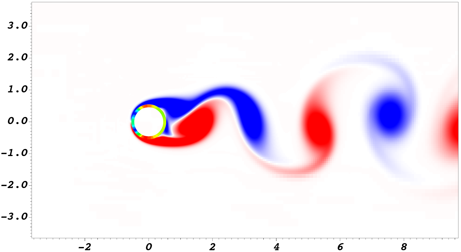
Figure 2: The vorticity field and the variable $\varepsilon_{\mathbf{X}}$ are visualized over a subset of the fluid domain at $t=100$. The top panel uses DG-IIM, while the bottom panel uses CG-IIM jump conditions.

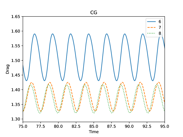
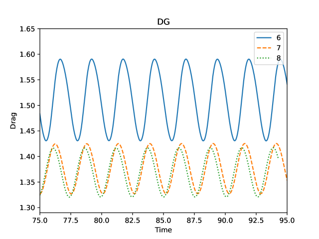
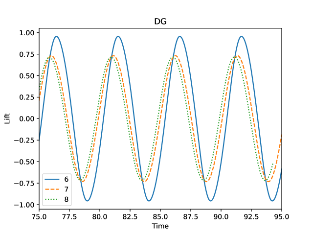
Figure 3: Time histories of lift and drag for flow past a circular cylinder for $\ell_{\text{max}}=\{6,7,8\}$. Both CG-IIM and DG-IIM exhibit convergence under grid refinement.

We quantify the simulation outputs using the nondimensionalized drag and lift coefficients, which are computed via

$$C_{\text{D}}=\frac{-\int_{\Gamma_{0}}F^{x}(\mathbf{X},t)\,{\mathrm{d}}s}{\frac{1}{2}\rho U^{2}D}$$ (18)

$${C_{\text{L}}}_{\textrm{}}=\frac{-\int_{\Gamma_{0}}F^{y}(\mathbf{X},t)\,{\mathrm{d}}s}{\frac{1}{2}\rho U^{2}D}$$ (19)

As a verification of the method, we conduct a grid convergence test (Figure 3). For both lift and drag coefficients, DG-IIM and CG-IIM both clearly converge to quantities within the range of previous literature values. For a discrete collection of times $\{t_{i}\}_{i=1}^{M}$ and the corresponding drag or lift coefficients and $C(t_{i})$, we compute the average coefficient as $C_{\text{avg}}=\frac{\max(C)+\min(C)}{2}$. Root-mean-squared drag and lift are computed as

$$C_{\text{rms}}=\sqrt{\frac{1}{M}\sum_{i=1}^{M}\left(C(t_{i})-C_{\text{avg}}\right)^{2}}.$$ (20)

The Strouhal number (St) is computed as $\text{St}=\frac{fD}{U}$, where $f$ is the frequency of vortex shedding, $D$ is the diameter of the cylinder, and $U$ is the horizontal inflow velocity.

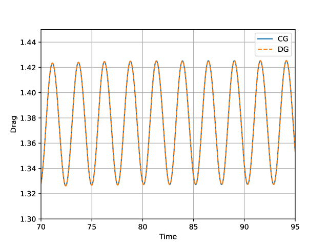
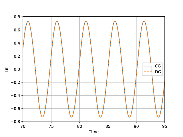
Figure 4: Comparison of drag (left) and lift (right) coefficients over time for both CG and DG formulations for circular cylinder flow with 7 levels of refinement. The absolute difference in $C_{{\text{D}_{\text{avg}}}}$, $C_{{\text{D}_{\text{rms}}}}$, $C_{{\text{L}_{\text{max}}}}$, and $C_{{\text{L}_{\text{rms}}}}$ between the two formulations are all less than 3e-5.

Figure 4 shows an agreement of these integrated quantities between the two methods.

Reference $C_{\text{D}}$ $C_{\text{L}}$ St Griffith and Luo[31] $1.360\pm 0.046$ $\pm 0.70$ 0.195 Liu et al. [32] $1.310\pm 0.049$ $\pm 0.69$ 0.192 Braza et al. [33] $1.400\pm 0.050$ $\pm 0.75$ 0.200 Calhoun[34] $1.172\pm 0.058$ $\pm 0.67$ 0.202 Present CG $1.370\pm 0.049$ $\pm 0.72$ 0.197 Present DG $1.370\pm 0.049$ $\pm 0.72$ 0.197

Table 1: Comparisons of lift and drag coefficients for ${Re}=200$ flow past a circular cylinder to results from prior studies.

The present lift and drag values fall within the range of literature values (Table 1). Griffith and Luo use an immersed boundary method with finite elements for structures and finite difference approximations for Eulerian variables. Liu et al. uses a finite differences with a turbulence model. Braza et al. use finite differences on the Navier Stokes equation specifically for cylinder flow. Calhoun uses an IIM with finite differences on a Cartesian grid[34].

4.2 Flow Past a Square Cylinder

This section considers flow past a stationary square cylinder of diameter $D=1$ centered at the origin of the computational domain $\Omega=[-15,45]\times[-30,30]$ with $L=60$. For $\mathbf{u}=(u,v)$, we use incoming flow velocity $\mathbf{}u=1$, and $v=\cos\left(\pi\frac{y}{L}\right)e^{-2t}$ to ensure that vortex shedding occurs at a consistent time. We set $\rho=1$ and $\mu=\frac{1}{{Re}}$, in which $Re$ is the Reynolds number. We use ${Re}=\frac{\rho UD}{\mu}=100$ to ensure that we observe vortex shedding. The effective number of grid cells on the $\ell^{\text{th}}$ level is ${n_{\ell}}=2^{\ell-1}n_{\text{c}}$, with $\ell_{\text{max}}=6$. For convergence studies, we vary $n_{\text{c}}=64$, $128$, $256$, and $512$. Comparisons to prior works, use the finest resolution considered, $n_{\text{c}}=512$. The time step size $\Delta t$ scales with $h_{\text{finest}}$ such that $\Delta t=\frac{h_{\text{finest}}}{20}$, in which $h_{\text{finest}}=\frac{L}{{n_{\ell{\text{max}}}}}$. For this time step size and grid spacing, the CFL number is approximately 0.05 once the model reaches periodic steady state. $\kappa$ and $\eta$ are scaled with the grid resolution on the finest level, such that $\kappa=\frac{C_{\kappa}}{h_{\text{finest}}}$ and $\eta=\frac{C_{\eta}}{h_{\text{finest}}}$ with $C_{\kappa}=3.413$ and $C_{\eta}=0.0036$ using a bisection method. The outflow boundary uses zero normal and tangential traction, and the top and bottom boundaries use zero tangential traction and $v=0$. Figure 5 gives a snapshot of the vorticity field and interface at $t=150$.

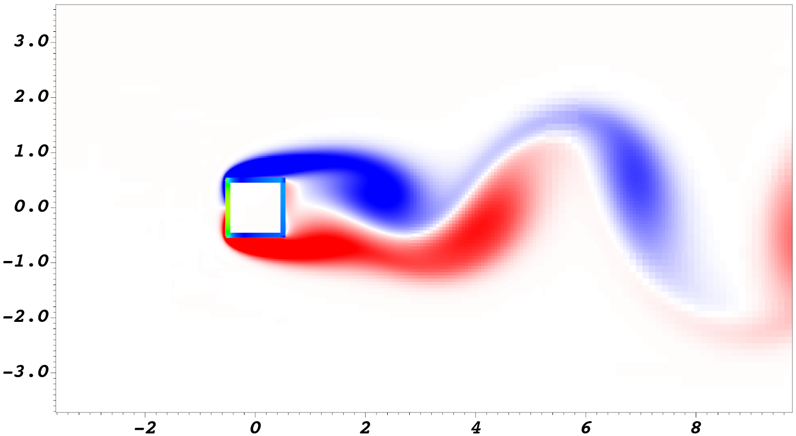
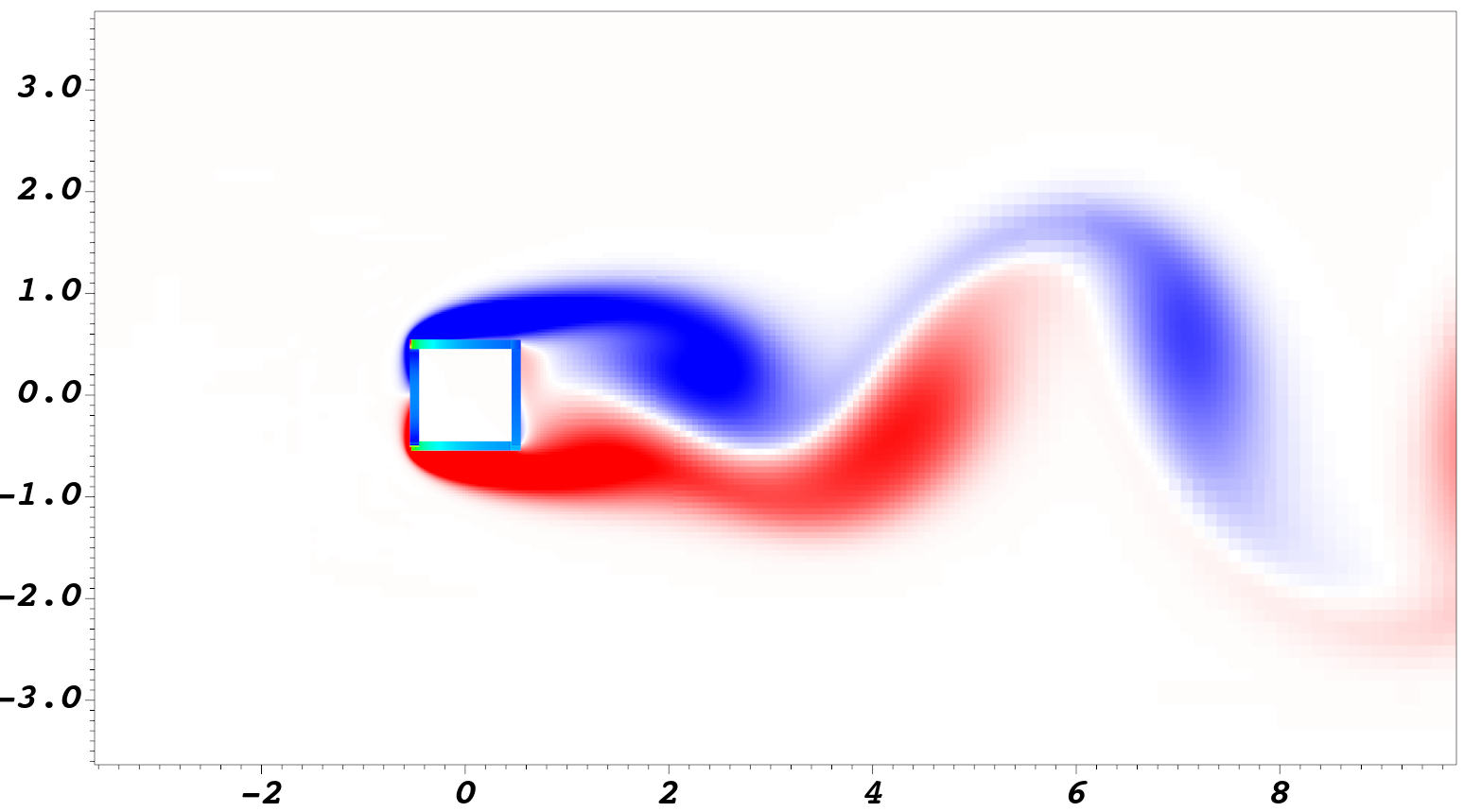
Figure 5: The vorticity field and the variable $\varepsilon_{\mathbf{X}}$ are visualized over a subset of the fluid domain at $t=150$. The top panel uses DG-IIM, while the bottom panel uses CG-IIM jump conditions.

We compare the discrepancy in interface configurations between CG-IIM and DG-IIM for various grid resolutions in Figure 6. Across all resolutions, the steady-state $\max(\varepsilon_{\mathbf{X}})$ for CG-IIM is twice as large as DG-IIM.

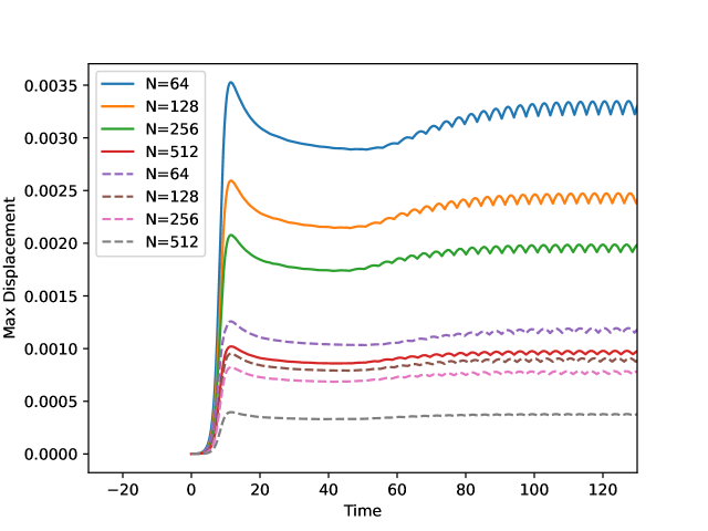
Figure 6: Flow past a stationary square cylinder time series for $\max(\varepsilon_{\mathbf{X}})$ using DG-IIM and CG-IIM formulations with $\kappa=\frac{C_{\kappa}}{h_{\text{finest}}}$, $\eta=\frac{C_{\eta}}{h_{\text{finest}}}$, and $n_{\text{c}}=\{64,128,256,512\}$ grid cells on the coarsest level with six levels of refinement. CG-IIM results use solid lines, and the DG-IIM results use dashed lines. The CG-IIM formulation has larger displacement for all grid discretizations.

Next, we study the convergence of the drag and lift coefficients under grid refinement (Figure 7).

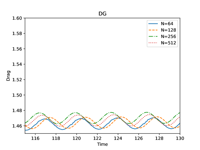
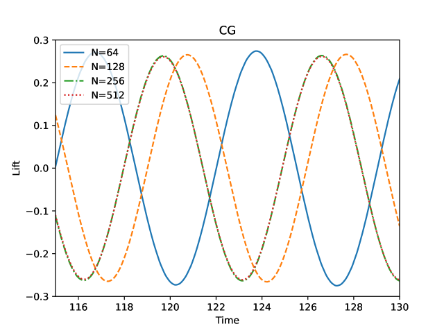
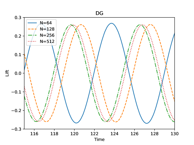
Figure 7: Time histories of lift and drag coefficients for flow past a square cylinder with $n_{\text{c}}=\{64,128,256,512\}$. The lift coefficient exhibits convergence for both methods. In contrast, the drag coefficient converges to literature values only while using DG-IIM.

Both CG-IIM and DG-IIM agree for lift coefficients across all grid resolutions. The DG-IIM drag coefficient converges with grid refinement, whereas the CG-IIM formulation does not achieve convergence on practical grids. We compare our most refined periodic steady state values to results from prior studies for $Re=100$ (Table 2). $C_{\text{L}_{\text{rms}}}$ agrees with prior studies for both formulations. $C_{\text{D}_{\text{avg}}}$ agrees with the range of literature values for DG-IIM, whereas CG-IIM yields a larger value. The Strouhal number for the DG-IIM formulation is closer to literature values than CG-IIM.

Reference $C_{\text{D}_{\text{avg}}}$ $C_{\text{L}_{\text{rms}}}$ St Sohankar et al.[35] 1.43 $0.15$ 0.146 Cheng et al.[36] $1.44$ $0.15$ 0.144 Lam et al.[37] 1.51 0.18 0.141 Berrone et al.[38] 1.48 0.18 0.145 Sen et al.[39] 1.52 0.19 0.145 Ryu & Iaccarino[40] 1.56 0.19 0.141 Present CG 1.57 0.18 0.138 Present DG 1.47 0.18 0.140

Table 2: Lift and drag coefficients, and Strouhal number comparison for $\text{Re}=100$ flow past a square cylinder.

Last, we compare our DG-IIM coefficients to values reported by Sen et al[39], who performed numerical experiments for flow past a square cylinder at a variety of Reynolds numbers. Table 3 shows close agreement in present calculations with those integrated quantities. Table 4 shows agreement in the circulation lengths for steady flows with cylinder diameter $D=1$.

Reynolds Number $C_{\text{L}_{\max}}$ $C_{\text{L}_{\text{rms}}}$ Sen et al. Present DG Sen et al. Present DG 60 0.13 0.124 0.09 0.0839 80 0.21 0.209 0.15 0.147 100 0.27 0.273 0.19 0.192 120 0.33 0.335 0.23 0.237 140 0.39 0.412 0.28 0.292

Reynolds Number $C_{\text{D}_{\text{avg}}}$ $C_{\text{D}_{\text{rms}}}$ Sen et al. Present DG Sen et al. Present DG 60 1.64 1.55 0.0009 0.0009 80 1.57 1.50 0.0028 0.0027 100 1.53 1.47 0.0055 0.0055 120 1.51 1.46 0.0096 0.0092 140 1.50 1.47 0.0143 0.0144

Table 3: Comparison of $C_{\text{L}_{\text{max}}}$, $C_{\text{L}_{\text{rms}}}$, $C_{\text{D}_{\text{avg}}}$, and $C_{\text{D}_{\text{rms}}}$ for flow past a square cylinder to literature values which use finite elements.

Reynolds Number L/D $C_{\text{D}}$ Sen et al. Present Sen et al. Present DG 5 2.806 2.786 4.9535 4.738 40 0.3166 0.323 1.7871 1.765

Table 4: Comparison of ratio of circulation length $L$ to square side length $D$, and drag coefficient for steady flows.

4.3 Rear Facing Angle

This test investigate the effects of increasingly acute angles in the interfacial geometry. We append a square cylinder of diameter $D=1$ with a rear-facing angle of varying acuteness. Six angles are considered, ranging from $\pi$ to $\frac{\pi}{9}$ (Figure 8). The square is centered at the origin of the computational domain $\Omega=[-15,45]\times[-30,30]$ with $L=16$. For $\mathbf{u}=(u,v)$, we use incoming flow velocity $\mathbf{}u=1$, and $v=\cos\left(\pi\frac{y}{L}\right)e^{-2t}$ to ensure that vortex shedding occurs at a consistent time. We set $\rho=1$ and $\mu=\frac{1}{{Re}}$, in which $Re$ is the Reynolds number. We use ${Re}=\frac{\rho UD}{\mu}=200$ to ensure that we observe vortex shedding. The effective number of grid cells on the $\ell^{\text{th}}$ level is ${n_{\ell}}=2^{\ell-1}n_{\text{c}}$, with $\ell_{\text{max}}=6$. The time step size $\Delta t$ scales with $h_{\text{finest}}$ such that $\Delta t=\frac{h_{\text{finest}}}{20}$, in which $h_{\text{finest}}=\frac{L}{{n_{\ell{\text{max}}}}}$. For this time step size and grid spacing, the CFL number is approximately 0.18 once the model reaches periodic steady state. We set $\kappa=156$ and $\eta=16$, which are determined using a bisection method. The outflow boundary uses zero normal and tangential traction, and the top and bottom boundaries use zero tangential traction and $v=0$.

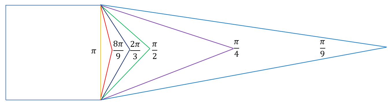
Figure 8: Square cylinder with rear-facing triangle, for $\theta=\left\{\frac{\pi}{9},\frac{\pi}{4},\frac{\pi}{2},\frac{2\pi}{3},\frac{8\pi}{9},\pi\right\}$

We vary $\theta$ in both CG-IIM and DG-IIM formulations. Twelve cases are run with a fixed $\kappa=156$ and $\eta=16$ to ensure the desired accuracy is achieved. In each case, we use a bisection method to find the largest stable $\Delta t$. For angles between $\frac{\pi}{9}$ and $\frac{8\pi}{9}$, discontinuous elements allow a 33% larger $\Delta t_{\max}$. The most noticable difference occurs at $\theta=\frac{\pi}{9}$. The angle is small enough that we are unable to determine a stable $\Delta t$ for CG-IIM. In contrast, for DG-IIM, our analysis identified the same maximum stable time step size $\Delta t_{\text{max}}$, independent of $\theta$ (Figure 9).

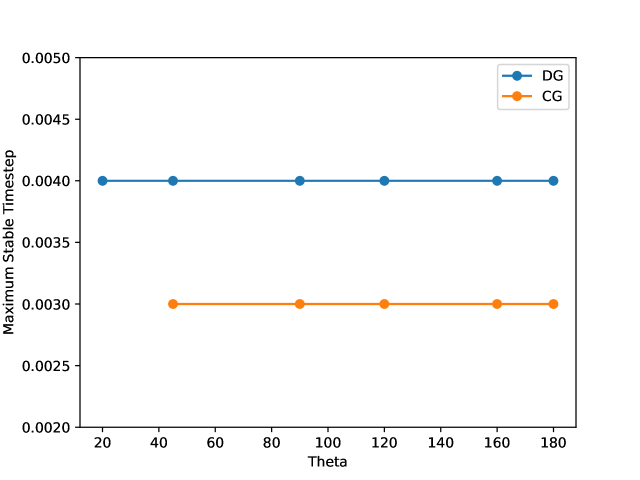
Figure 9: Maximum stable time step size for a square cylinder with a rear-facing triangle for $\kappa=156$ and $\eta=16$. CG formulation for $\theta=20$ degrees ($\frac{\pi}{9}$ radians) could not yield a stable time step size with the given parameters.

As long as the angle is sufficiently large, there is no variation in stability between different degrees of acuteness for CG-IIM. For all angles, the DG formulation provides a larger $\Delta t$ for fixed $\kappa$.

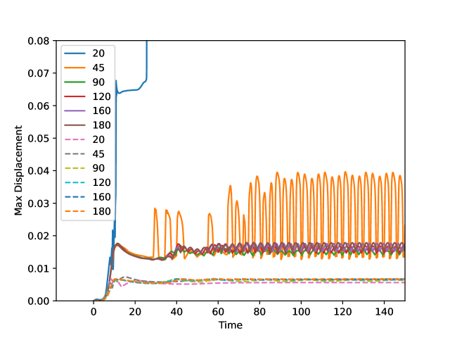
Figure 10: Time series of $\max(\varepsilon_{\mathbf{X}})$ for various angles (degrees). CG uses solid lines, and DG uses dashed lines. The CG formulation is not suitable for the most acute geometries.

Figure 10 show the maximum discrepancy $\max(\varepsilon_{\mathbf{X}})$ obtained by fixing $\kappa=156$ and $\eta=16$. The $\max(\varepsilon_{\mathbf{X}})$ shows minimal variation across the angles using DG jump conditions. However, the two most acute geometries exhibit large spikes in displacement for the CG formulation. To compare the effects of the more acute geometry on the parameter sets, we vary $\kappa$ with CG jump conditions. It is possible to obtain approximately the same $\max(\varepsilon_{\mathbf{X}})$ as DG by increasing $\kappa$ by a factor of 4 (Figure 11). However, such an increase requires a proportional reduction in $\Delta t$.

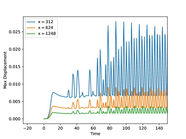
Figure 11: Time series of $\max(\varepsilon_{\mathbf{X}})$ for a 45 degree angle using the CG formulation. The upper bound on $\max(\varepsilon_{\mathbf{X}})$ may be reduced by increasing $\kappa$.

4.4 Flow Past a Sphere

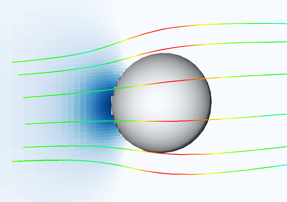
Figure 12: Pressure field slice of the $x-y$ plane of flow past a unit sphere at Re=100 using DG jump handling. Streamlines are colored by magnitude of velocity.

This section considers flow past a sphere (Figure 12) of diameter $D=1$ centered at the origin of the computational domain $\Omega=[-6,18]\times[-12,12]\times[-12,12]$ with $L=24$. For $\mathbf{u}=(u,v,w)$, we use incoming flow velocity $\mathbf{}u=1$, $v=0$,$w=0$. We set $\rho=1$ and $\mu=\frac{1}{{Re}}$, in which $Re$ is the Reynolds number. We use various Reynolds numbers to compare to data from Jones and Clarke[41], namely ${Re}=\frac{\rho UD}{\mu}=40$, $60$, $80$, $100$, $120$, and $140$. The effective number of grid cells on the $\ell^{\text{th}}$ level is ${n_{\ell}}=2^{\ell-1}n_{\text{c}}$, with $\ell_{\text{max}}=7$. The time step size $\Delta t$ scales with $h_{\text{finest}}$ such that $\Delta t=\frac{h_{\text{finest}}}{20}$, in which $h_{\text{finest}}=\frac{L}{{n_{\ell{\text{max}}}}}$. For this time step size and grid spacing, the CFL number is approximately 0.056 once the model reaches steady state. $\kappa=250$ and $\eta=1$, which are computed using a bisection method. The boundaries perpendicular to the $y$ and $z$ axes use the zero traction and no-penetration conditions. The outflow boundary uses zero normal and tangential traction.

$C_{\text{D}}$ Re Present CG Present DG Jones and Clark[41] 40 1.79 1.77 1.79 60 1.42 1.41 1.42 80 1.21 1.20 1.22 100 1.08 1.07 1.087 120 0.98 0.97 0.99 140 0.91 0.90 0.92

Table 5: Comparison of the steady state drag coefficient for flow past a unit sphere across various Reynolds numbers for CG-IIM and DG-IIM jump conditions and literature values.

Table 5 shows agreement in $C_{\text{D}}$ between present DG-IIM computations and Jones and Clarke [41]. Max($\|\varepsilon_{\mathbf{X}}\|$) was measured at ${Re}=100$ for both CG-IIM and DG-IIM. Similar to the two dimensional circular cylinder test, there was little difference between the two approaches. Max($\|\varepsilon_{\mathbf{X}}\|$) was 0.0029 for DG-IIM and 0.00288 for CG-IIM.

4.5 Flow Past a Cube

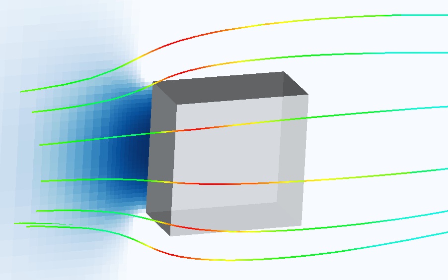
Figure 13: Pressure field slice of the $x-y$ plane of flow past a unit cube at Re=100 using DG jump handling. Streamlines are colored by magnitude of velocity.

This section considers flow past a cube (Figure 13) of diameter $D=1$ centered at the origin of the computational domain $\Omega=[-8.75,26.25]\times[-17.5,17.5]\times[-17.5,17.5]$ with $L=35$. For $\mathbf{u}=(u,v,w)$, we use incoming flow velocity $\mathbf{}u=1$, $v=0$, $w=0$. We set $\rho=1$ and $\mu=\frac{1}{{Re}}$, in which $Re$ is the Reynolds number. We use various Reynolds numbers to compare to data from Saha et al.[42], namely ${Re}=\frac{\rho UD}{\mu}=50$, $100$, $150$, and $200$. The effective number of grid cells on the $\ell^{\text{th}}$ level is ${n_{\ell}}=2^{\ell-1}n_{\text{c}}$, with $\ell_{\text{max}}=7$. The time step size $\Delta t$ scales with $h_{\text{finest}}$ such that $\Delta t=\frac{h_{\text{finest}}}{10}$, in which $h_{\text{finest}}=\frac{L}{{n_{\ell{\text{max}}}}}$. For this time step size and grid spacing, the Courant-Friedrichs-Lewy (CFL) number is approximately 0.03 once the model reaches steady state. We use $\kappa=250$ and $\eta=1$, which are determined using a bisection method. The boundaries perpendicular to the $y$ and $z$ axes use the zero traction and no-penetration conditions. The outflow boundary uses zero normal and tangential traction.

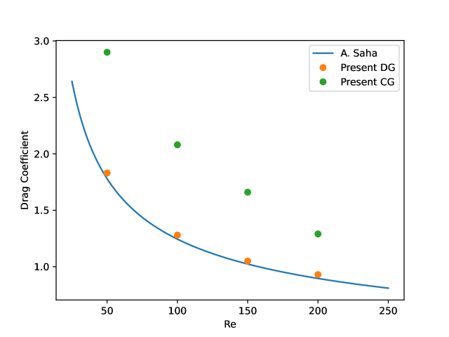
Figure 14: Comparison of present CG-IIM and DG-IIM computations with the Reynolds-drag curve fit from Saha et al[42].

Figure 14 shows the agreement between current DG-IIM simulations and data from Saha et al.[42] for the steady state drag coefficient at various Reynolds numbers. CG-IIM formulation overestimates $C_{\text{D}}$ at all simulated Reynolds numbers. The max($\varepsilon_{\mathbf{X}}$) was measured at $\text{Re}=100$ for both CG-IIM and DG-IIM. Similar to the two dimensional square cylinder test, there was noticable difference for sharp geometries. The max($\varepsilon_{\mathbf{X}}$) was 0.004 for DG and 0.0222 for CG.

5 Discussion

This study demonstrates that the IIM with DG-projected jump conditions is an effective approach to computing external flows around structures with sharp edges. The study also demonstrates that, for smooth interface geometries, the DG-IIM approach provides accuracy and efficiency that are comparable to our initial CG-IIM scheme. An important advantage of the DG-IIM representation of jump conditions is that it allows for larger stable time steps than CG-IIM for non-smooth geometries. For the rear-facing angle model, geometry with acute angles less than or equal to $\frac{\pi}{4}$, restrictions on $\kappa$, and as a result, $\max(\Delta t)$ become more severe for CG-IIM representations, whereas DG-IIM’s maximum stable time step size need not be decreased to maintain stability. These results suggest that DG-IIM is more suitable to dealing with immersed interfaces with sharp features geometry, which are common in models of engineered structures. Future extensions of the method could involve implementing higher order jump conditions, or representing the geometry itself with a DG-IIM formulation.

References

- [1] B. E. Griffith. Immersed boundary model of aortic heart valve dynamics with physiological driving and loading conditions. International Journal for Numerical Methods in Biomedical Engineering, 28(3):317–345, 2012.
- [2] C. S. Peskin. Flow patterns around heart valves: A numerical method. Journal of Computational Physics, 10(2):252–271, 1972.
- [3] Y. Zeng, Y. Wang, D. Yang, and Q. Chen. Immersed boundary methods for simulations of biological flows in swimming and flying bio-locomotion: A review. Applied Sciences, 13(7):4208, 2023.
- [4] E. M. Kolahdouz, D. R. Wells, S. Rossi, K. I. Aycock, B. A. Craven, and B. E. Griffith. A sharp interface lagrangian-eulerian method for flexible-body fluid-structure interaction. Journal of Computational Physics, 448:112174, 2023.
- [5] A. Mayo. The fast solution of poisson’s and the biharmonic equations on irregular regions. SIAM Journal on Numerical Analysis, 21(2):285–299, 1984.
- [6] R. J. LeVeque and Z. Li. The immersed interface method for elliptic equations with discontinuous coefficients and singular sources. SIAM Journal on Numerical Analysis, 31(4):1019–1044, 1994.
- [7] L. Lee and R. J. LeVeque. An immersed interface method for incompressible navier–stokes equations. SIAM Journal on Scientific Computing, 25(3):832–856, 2003.
- [8] Z. Li and M. Lai. The immersed interface method for the navier–stokes equations with singular forces. Journal of Computational Physics, 171(2):822–842, 2001.
- [9] S. Xu and Z. Wang. Systematic derivation of jump conditions for the immersed interface method in three-dimensional flow simulation. SIAM Journal on Scientific Computing, 27:1948–1980, 2006.
- [10] N. Thekkethil and A. Sharma. Level set function–based immersed interface method and benchmark solutions for fluid flexible-structure interaction. International Journal for Numerical Methods in Fluids, 91(3):134–157, 2019.
- [11] J. Xu, W. Shi, W. Hu, and J. Huang. A level-set immersed interface method for simulating the electrohydrodynamics. Journal of Computational Physics, 400:108956, 2020.
- [12] E. M. Kolahdouz, A. P. Singh Bhalla, B. A. Craven, and B. E. Griffith. An immersed interface method for discrete surfaces. Journal of Computational Physics, 400:108854, 2020.
- [13] E. M. Kolahdouz, A. P. S. Bhalla, L. N. Scotten, B. A. Craven, and B. E. Griffith. A sharp interface lagrangian-eulerian method for rigid-body fluid-structure interaction. Journal of Computational Physics, 443:110442, 2021.
- [14] D. V. Le, B. C. Khoo, and J. Peraire. An immersed interface method for viscous incompressible flows involving rigid and flexible boundaries. Journal of Computational Physics, 220(1):109–138, 2006.
- [15] B. Cockburn. Discontinuous galerkin methods for computational fluid dynamics. In Encyclopedia of Computational Mechanics Second Edition, pages 1–63. John Wiley & Sons, Ltd, 2017.
- [16] C. S. Peskin and B. F. Printz. Improved volume conservation in the computation of flows with immersed elastic boundaries. Journal of Computational Physics, 105(1):33–46, 1993.
- [17] B. E. Griffith and N. A. Patankar. Immersed methods for fluid–structure interaction. Annual Review of Fluid Mechanics, 52:421–448, 2020.
- [18] B. E. Griffith. On the volume conservation of the immersed boundary method. Communications in Computational Physics, 12(2):401–432, 2012.
- [19] B. E. Griffith. An accurate and efficient method for the incompressible navier–stokes equations using the projection method as a preconditioner. Journal of Computational Physics, 228(20):7565–7595, 2009.
- [20] W. J. Rider, J. A. Greenough, and J. R. Kamm. Accurate monotonicity- and extrema-preserving methods through adaptive nonlinear hybridizations. Journal of Computational Physics, 225(2):1827–1848, 2007.
- [21] P. Colella and P. R. Woodward. The piecewise-parabolic method (ppm) for gas-dynamical simulations. Journal of Computational Physics, 54:174–201, 1984.
- [22] IBAMR: an adaptive and distributed-memory parallel implementation of the immersed boundary method. https://github.com/IBAMR/IBAMR.
- [23] SAMRAI: Structured adaptive mesh refinement application infrastructure. http://www.llnl.gov/CASC/SAMRAI.
- [24] S. Balay, S. Abhyankar, M. F. Adams, J. Brown, P. Brune, K. Buschelman, L. Dalcin, V. Eijkhout, W. D. Gropp, D. Kaushik, M. G. Knepley, D. A. May, L. C. McInnes, R. T. Mills, T. Munson, K. Rupp, P. Sanan, B. F. Smith, S. Zampini, and H. Zhang. Petsc web page, 2018. http://www.mcs.anl.gov/petsc.
- [25] S. Balay, S. Abhyankar, M. F. Adams, J. Brown, P. Brune, K. Buschelman, L. Dalcin, V. Eijkhout, W. D. Gropp, D. Kaushik, M. G. Knepley, D. A. May, L. C. McInnes, R. T. Mills, T. Munson, K. Rupp, P. Sanan, B. F. Smith, S. Zampini, and H. Zhang. Petsc users manual. Technical Report Tech. Rep. ANL-95/11 - Revision 3.9, Argonne National Laboratory, 2018. http://www.mcs.anl.gov/petsc.
- [26] S. Balay, W. D. Gropp, L. C. McInnes, and B. F. Smith. Efficient management of parallelism in object-oriented numerical software libraries. In E. Arge, A. M. Bruaset, and H. P. Langtangen, editors, Modern Software Tools in Scientific Computing, pages 163–202. Birkhauser Press, 1997.
- [27] Hypre: high performance preconditioners. http://www.llnl.gov/CASC/hypre.
- [28] R. D. Falgout and U. M. Yang. hypre: A library of high performance preconditioners. In International Conference on Computational Science, pages 632–641. Springer, 2002.
- [29] libMesh: a C++ finite element library. http://libmesh.github.io.
- [30] B. S. Kirk, J. W. Peterson, R. H. Stogner, and G. F. Carey. libMesh: A C++ library for parallel adaptive mesh refinement/coarsening simulations. Engineering Computations, 22(3):237–254, 2006.
- [31] B. E. Griffith and X. Y. Luo. Hybrid finite difference/finite element immersed boundary method. International Journal for Numerical Methods in Biomedical Engineering, 33(12):0, 2017.
- [32] C. Liu, X. Zheng, and C. H. Sung. Preconditioned multigrid methods for unsteady incompressible flows. Journal of Computational Physics, 139(1):35–57, 1998.
- [33] M. Braza, P. Chassaing, and H. Ha Minh. Numerical study and physical analysis of the pressure and velocity fields in the near wake of a circular cylinder. Journal of Fluid Mechanics, 165:79–130, 1986.
- [34] D. Calhoun. A cartesian grid method for solving the two-dimensional streamfunction-vorticity equations in irregular regions. Journal of Computational Physics, 176(2):231–275, 2002.
- [35] A. Sohankar, C. Norberg, and L. Davidson. Numerical simulation of unsteady low-reynolds number flow around rectangular cylinders at incidence. Journal of Wind Engineering and Industrial Aerodynamics, 69-71:189–201, 1997.
- [36] M. Cheng, D. S. Whyte, and J. Lou. Numerical simulation of flow around a square cylinder in uniform-shear flow. Journal of Fluids and Structures, 23(2):207–226, 2007.
- [37] K. Lam, Y. F. Lin, L. Zou, and Y. Liu. Numerical study of flow patterns and force characteristics for square and rectangular cylinders with wavy surfaces. Journal of Fluids and Structures, 28:359–377, 2012.
- [38] S. Berrone, V. Garbero, and M. Marro. Numerical simulation of low-reynolds number flows past rectangular cylinders based on adaptive finite element and finite volume methods. Computers & Fluids, 40(1):92–112, 2011.
- [39] S. Sen, S. Mittal, and G. Biswas. Flow past a square cylinder at low reynolds numbers. International Journal for Numerical Methods in Fluids, 67(9):1160–1174, 2011.
- [40] S. Ryu and G. Iaccario. Vortex-induced rotations of a rigid square cylinder at low reynolds numbers. Journal of Fluid Mechanics, 813:482–507, 2017.
- [41] D. A. Jones and D. B. Clarke. Simulation of flow past a sphere using the fluent code, 2008. Australian Defence Science and Technology Organisation.
- [42] A. K. Saha. Three-dimensional numerical simulations of the transition of flow past a cube. Physics of Fluids, 16(5):1630–1646, 2004.