Automated Planning Domain Inference for Task and Motion Planning

Abstract

Task and motion planning (TAMP) frameworks address long and complex planning problems by integrating high-level task planners with low-level motion planners. However, existing TAMP methods rely heavily on the manual design of planning domains that specify the preconditions and postconditions of all high-level actions. This paper proposes a method to automate planning domain inference from a handful of test-time trajectory demonstrations, reducing the reliance on human design. Our approach incorporates a deep learning-based estimator that predicts the appropriate components of a domain for a new task and a search algorithm that refines this prediction, reducing the size and ensuring the utility of the inferred domain. Our method is able to generate new domains from minimal demonstrations at test time, enabling robots to handle complex tasks more efficiently. We demonstrate that our approach outperforms behavior cloning baselines, which directly imitate planner behavior, in terms of planning performance and generalization across a variety of tasks. Additionally, our method reduces computational costs and data amount requirements at test time for inferring new planning domains.

I Introduction

Robot autonomy that generalizes to diverse environments requires efficient integration of complex real-time perception, decision-making, and motion planning. Existing motion planning reaches its limits in complex and high-dimensional environments [8, 21, 23, 26, 33] that are frequently encountered in modern robot applications [16]. Task and motion planning (TAMP) frameworks address this challenge by employing high-level task planners to discretize a complex planning task into a sequence of manageable sub-tasks that low-level motion planners can complete.

While existing TAMP frameworks have solved many complex and long-horizon tasks in robotics [7, 17], they rely heavily on human-designed planning domains, which are sets of logical rules and constraints that provide a basis for high-level task plans. Planning domains are restricted to predefined decision spaces and cannot easily be adapted to new tasks. This limitation drives the need for automated solutions that generate planning domains by leveraging information about existing, similar domains. We aim to develop a method that learns the relationships between tasks and their respective planning domains from training data, enabling the automatic generation of a new planning domain based on just one or a few demonstrations from humans.

This paper introduces an automated planning domain inference method that generates planning domains for new TAMP problems in a one-shot or few-shot manner, using demonstrations of continuous state-action trajectories. Our approach uses deep learning to predict domains for new tasks. To further improve the feasibility and planning efficiency of the planning domain, we combine these predictions with search algorithms to reduce the size of the planning domain to the smallest possible while ensuring that the generated domains are effective and reliable.

The primary contribution of this paper is (1) a graph attention network (GAT) trained on a small set of demonstrations to efficiently predict the planning domain for new tasks; (2) a guided generate-and-test search algorithm to refine the predicted planning domain, ensuring that planning is both feasible and efficient; (3) a framework that is deployable on a real robot that integrates GAT prediction and search to infer the planning domain for new tasks, requiring only a single human demonstration. We evaluate our method and compare it to existing baselines in 12 different environments. Our method significantly improves planning performance, generalizability, and computational costs.

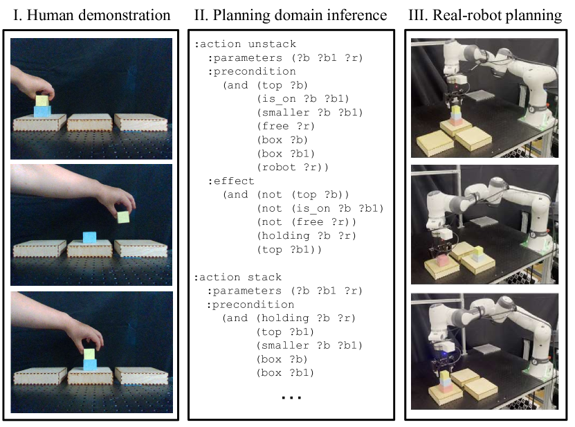
Figure 1: Illustration of the general idea of this work: (1) One or a few human demonstrations for task execution are provided. 3D perception is used to extract object poses and interactions. (2) Plausible planning domains are inferred based on human demonstrations. (3) The generated domain is used for Task and Motion Planning and execution on real robots.

II Related Work

II-A Learning to Plan for Faster Task and Motion Planning

Recent advances in machine learning have brought new approaches to task and motion planning. Learning-based TAMP methods often train policies that either accelerate or replace traditional planners. Recent research highlights the effectiveness of both supervised learning and reinforcement learning. Supervised learning methods demonstrate great ability to accelerate planning, but they often require extensive demonstration data and are conditioned to specific environments [12, 13, 15, 27]. This limits their ability to generalize across different environment settings or goals [2, 20, 34, 32]. Reinforcement learning, as another major learning-based TAMP method in recent years, assists in accelerating the planning speed and enhances adaptability to dynamic and uncertain environments [1, 9, 25, 31]. However, creating a well-defined learning environment for complex TAMP problems, in simulation or in the real world, can be challenging. This reduces the applicability of reinforcement learning in TAMP scenarios [29, 33].

II-B Learning Planning Domains

Recognizing the discussed limitations, researchers have increasingly shifted their focus toward learning planning domains. The mainstream learning-based methods in TAMP, designed to replicate the planner’s behavior, implicitly learns both the planning domain and the search algorithm. Focusing solely on learning the planning domain and integrating it with existing search algorithms reduces the burden on the learning algorithm.

Success in learning logical predicates from the environment  [10, 22, 28] facilitates the study of automatic generation of planning domains [14]. Automatic planning domain generation uses pre-existing logical predicates and actions to create planning domains autonomously. Recent studies have demonstrated that learning a planning domain enhances generalizability and adaptability compared to directly learning a TAMP planner [3]. However, existing methods encounter the challenges of high search costs and the requirement of a relatively large dataset [14, 28].

Our method is closely related to that of Kumar et al. [14], which identifies necessary preconditions and postconditions of an operator through a hill-climbing search. However, our method attempts to generate a full planning domain instead of merely operators (actions). Furthermore, rather than starting the search from scratch, our approach leverages transferable knowledge from existing planning domains, significantly accelerating the generation of domains and reducing the number of demonstrations required during execution. As a result, we are able to generate new planning domains for unseen tasks in a one-shot or few-shot manner.

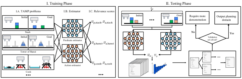
Figure 2: The overall framework of domain inference. Left: The training phase of our method. Right: the testing phase of our method.

III Problem setting

The standardized planning language used in this work is Planning Domain Definition Language (PDDL)  [19]. For a given task, the object set $\mathbf{O}=\langle o_{1},o_{2},\dots,o_{n}\rangle$ includes all relevant objects in the environment, with objects $o\in\mathbf{O}$ are references to entities in the planning problem [11]. The state function $s:\mathbf{O}\times\mathbf{T}\rightarrow\mathcal{R}^{d\times n}$ provides the continuous state of an object, where $\mathbf{T}$ is the time indices denoting the time at which the state of an object is evaluated. This state is defined by continuous properties, such as pose and temperature.

Definition III.1 (Full predicate set).

The full predicate set $\mathbf{P}$ is a set that encompasses all the predicates required to solve a set of TAMP problems.

Each predicate $\mathbf{\mathit{p}}\in\mathbf{P}$ defines a logical property, condition, or relationship among objects (e.g., (is_on ?$o_{1}$ ?$o_{2}$)) via a classifier function that outputs true or false given the continuous state $p(s(o_{1},t),s(o_{2},t),\dots)\in\{\text{true; false}\}$. A ground atom $x$ is a predicate combined with the objects and the classification result (e.g., (is_on $o_{1}$ $o_{2}$)). The logical state of an environment is a collection of all ground atoms for objects in the environment $\mathbf{X}=\langle\mathbf{\mathit{x_{1}}},\mathbf{\mathit{x_{2}}},\mathbf{\mathit{x_{3}}},\dots,\mathbf{\mathit{x_{n}}}\rangle$.

Definition III.2 (Full action set).

The full action set $\mathbf{A}$ is a set of actions that logically describe possible actions the robot may execute for a set of TAMP problems.

Each logical action $\mathbf{\mathit{a}}\in\mathbf{A}$ has a corresponding precondition $\mathbf{Pre}=\langle\mathbf{\mathit{p_{1}}},\mathbf{\mathit{p_{2}}},...\rangle$, which is a set of predicates that must be true to trigger the action, and a postcondition $\mathbf{Eff}=\langle\mathbf{\mathit{p_{1}}},\mathbf{\mathit{p_{2}}},...\rangle$, which is a set of predicates that indicates the change in the logical environmental state after the action is executed. The transition between logical states before and after the actions is considered to be deterministic, $\mathbf{X_{\mathrm{before}}}\times\mathbf{\mathit{a}}\rightarrow\mathbf{X_{\mathrm{after}}}$. A task plan $\mathit{\pi}=\langle\mathbf{\mathit{a_{1}}},\mathbf{\mathit{a_{2}}},\mathbf{\mathit{a_{3}}},...,\mathbf{\mathit{a_{n}}}\rangle$ is a sequence of logical actions that change the initial logical environmental state to the goal logical environmental state. A (logical) trajectory $\mathbf{\tau}$ is the sequence of logical environmental state and logical action at each step during task execution, $\mathbf{\tau}=\langle(\mathbf{X_{1}},a_{1}),(\mathbf{X_{2}},a_{2}),\dots,(\mathbf{X_{n}},a_{n})\rangle$.

Definition III.3 (Full motion planner set).

The full motion planner set $\mathbf{C}$ is a set of motion planners that produce the corresponding trajectories for actions in $\mathbf{A}$.

For each $\mathbf{\mathit{a}}\in\mathbf{A}$, there is a corresponding $\mathbf{\mathit{c}}\in\mathbf{C}$ that verifies the feasibility of motion plans for the action and generates the plan if feasible. For example, the corresponding motion planner for the action ‘Pick’ will generate a collision-free trajectory for the robot to grasp an object and lift it from the table.

Using the concept defined above, we can now define a TAMP problem. Any TAMP problem $q$ can be defined by the object set, the full predicate set, the full action set, the initial logical environmental state, and the goal logical environmental state, $q=\langle\mathbf{O},\mathbf{P},\mathbf{A},\mathbf{X_{\mathrm{init}}},\mathbf{X_{\mathrm{goal}}},\rangle$. A TAMP problem set $\mathbf{Q}$ is a set of unsolved TAMP problems $\mathbf{Q}=\langle q_{1},q_{2},\dots\rangle$.

The planning domain $\mathbf{D}$ associated with a task is characterized by a set of logical predicates $\mathbf{P_{\mathbf{D}}}\subseteq\mathbf{P}$, a set of logical actions $\mathbf{A_{\mathbf{D}}}\subseteq\mathbf{A}$, and the corresponding motion planner set $\mathbf{C_{\mathbf{D}}}\subseteq\mathbf{C}$. Formally, the planning domain is defined as $\mathbf{D}=\langle\mathbf{P_{\mathbf{D}}},\mathbf{A_{\mathbf{D}}},\mathbf{C_{\mathbf{D}}}\rangle$. The domain set $\omega_{\mathbf{D}}$ contains all the names of the predicates in $\mathbf{P_{\mathbf{D}}}$ and actions in $\mathbf{A_{\mathbf{D}}}$. The planning domain $\mathbf{D}$ can be constructed from the domain set $\omega_{\mathbf{D}}$ by designing the preconditions and postconditions for each action and writing the domain into a PDDL file following the PDDL syntax.

A TAMP problem $q$ can be addressed using various planning domains, each with differing performance based on its quality. To evaluate expected performance, we propose two criteria: completeness and optimality, to measure how well a planning domain solves the TAMP problem.

Definition III.4 (Complete Domain).

A complete domain is a domain that includes all predicates and actions needed to solve the TAMP problem.

Definition III.5 (Optimal domain).

An optimal domain is a complete domain that contains the least number of predicates and actions.

Given $\mathbf{A}$, $\mathbf{P}$, and $\mathbf{C}$, at the testing phase, our system aims at utilizing one (or a few) example trajectory $\mathbf{\tau_{e}}$ and a validation problem set containing $m$ unsolved TAMP problems, $\mathbf{Q}_{v}=\langle q_{1},q_{2},\dots,q_{m}\rangle$, to produce the optimal planning domain $\mathbf{D_{\mathrm{optm}}}=\langle\mathbf{P_{\mathrm{optm}}},\mathbf{A_{\mathrm{optm}}},\mathbf{C_{\mathrm{optm}}}\rangle$ that can reproduce $\mathbf{\tau_{e}}$ and generalize to similar TAMP tasks, even with shuffled object poses and varied object numbers.

IV Methodology

As shown in Figure 2, our method proceeds in two phases: a training phase and a testing phase. In the former, we use a training dataset of TAMP problems to learn a domain estimator that outputs the relevance of predicates and actions. In the testing phase, we use one or a few demonstration trajectories and a validation problem set to generate an optimal planning domain that does not violate the logical sequences in the demonstration trajectories.

More concretely, in Figure 2.I the training dataset includes information on TAMP problems with their associated planning domains. The predicate and action estimators output a relevance score $u\in[0,1]$ for each predicate and action, estimating their relevance of being part of the planning domain for a given problem $q$. The scores of predicates (actions) are denoted as $u_{\mathrm{p}}\in\mathit{U_{\mathrm{p}}}$ ($u_{\mathrm{a}}\in\mathit{U_{\mathrm{a}}}$), where the predicate (action) score set $\mathit{U_{\mathrm{p}}}$ ( $\mathit{U_{\mathrm{a}}}$) contains the score for all predicates (actions).

During testing, the inputs are an example trajectory $\mathbf{\tau_{e}}$ and a validation problem set $\mathbf{Q}_{v}$. As shown in Figure 2.II, the testing phase involves two main steps. First, the human demonstration (sensory data or human inputs) is converted into $\mathbf{\tau_{e}}$ to predict a distribution of relevant planning domains. Second, the predicted planning domains are refined by a search algorithm to find the optimal planning domain. If any of the domains explored during the search successfully solve all problems in the validation set $\mathbf{Q}_{v}$, the system returns the optimal domain $\mathbf{D_{\mathrm{optm}}}$. Otherwise, additional example trajectories of the same task are required.

IV-A Predicate and Action Estimators

To train the predicate and action estimators, the initial and goal logical states $(\mathbf{X_{\mathrm{init}}},\mathbf{X_{\mathrm{goal}}})$ of a TAMP problem are represented as scene graphs, with nodes representing objects. As is shown in Figure 3, unary predicates defining individual object states are encoded as Boolean values in the node feature vector. Binary predicates representing relationships between objects are formulated as edges connecting nodes with one-hot encoded edge features. If predicates involve more than two objects, the objects are connected in pairs, with each connection sharing the same edge feature.

Each estimator processes the scene graphs through several graph attention convolution layers (GATConv). The output from the final GATConv layer is passed through a multilayer perceptron (MLP). A sigmoid function is applied at the end to produce an output vector with elements between 0 and 1. Each output vector element indicates the relevance score of a specific predicate $p\in\mathbf{P}$ (action $a\in\mathbf{A}$) with respect to the input scene graph. The relevance score for a domain set is computed in the following manner:

$$u_{\mathbf{D}}=\prod_{p\in\omega_{\mathbf{D}}}u_{\mathrm{p}}\prod_{p\notin\omega_{\mathbf{D}}}(1-u_{\mathrm{p}})\prod_{a\in\omega_{\mathbf{D}}}u_{\mathrm{a}}\prod_{a\notin\omega_{\mathbf{D}}}(1-u_{\mathrm{a}})$$ (1)

In Equation 1, $u_{\mathrm{p}}$ represents the score for a predicate, while $u_{\mathrm{a}}$ represents the score for an action. The scores for all possible domain sets can be computed using Equation 1. The domain set with the highest relevance score is denoted as $\omega_{\mathbf{D}}^{\mathrm{top}}$. The predicates and actions excluded from $\omega_{\mathbf{D}}^{\mathrm{top}}$ are ranked by their relevance score in a descending manner in a priority list $\mathbf{\mathit{L}}$. Similar score computation schemes can be found in learning-based incremental planning methodologies [27].

IV-B Dataset Generation

To effectively train the predicate and action estimator, we require a training dataset of TAMP problems and their associated planning domains. This dataset is generated using a sampling-based approach that randomly samples various planning problems in the simulation environment. Each TAMP problem is labeled with the relevant predicates and actions for their planning domain, assigning a score of 1 to those crucial for solving the problem and a score of 0 to irrelevant ones. The solvability of each TAMP problem is verified via a traditional TAMP planner  [12] deployed on a compute cluster.

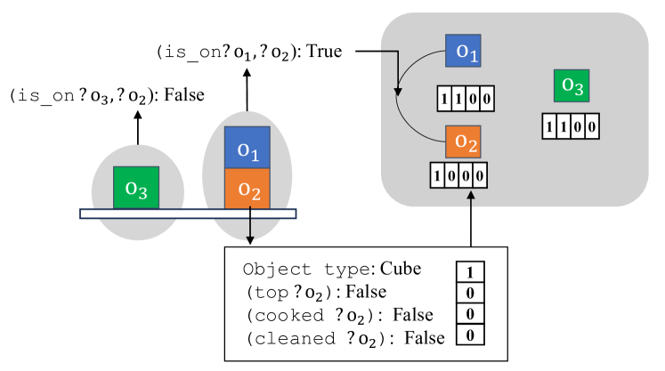
Figure 3: Example on formulating logical states as scene graphs: (1) Unary predicates: Using the orange cube as an example, object ‘cube’ has an index of 1, (top, $?o$), (cleaned, $?o$) and (cooked, $?o$) are all false. The feature node vector becomes $[1,0,0,0]$. We repeat this process for the other cubes to obtain the corresponding node features (2) Binary predicates: For example, the predicate (is_on, $?o_{1}$, $?o_{2}$ ) is true for the blue and orange cubes. Thus, an edge is formulated to connect them. Meanwhile, (is_on, $?o_{3}$, $?o_{2}$ ) is false, so there is no edge between green and orange cube.

IV-C Precondition and Postcondition Generation

In the testing phase, we obtain $\omega_{\mathbf{D}}^{\mathrm{top}}$ from the predicate and action estimators. Then, we must convert $\omega_{\mathbf{D}}^{\mathrm{top}}$ into an executable PDDL domain $\mathbf{D_{\mathrm{top}}}$ by determining the preconditions and postconditions for each action. This process depends on finding the commonalities across instances of the same action from the human demonstration.

Definition IV.1 (Pre-image).

The logical world state for the last time step before the action is triggered.

Definition IV.2 (Post-image).

The logical world state for the first time step after the action is completed.

The precondition is determined by identifying the intersections of the pre-images of the same action across multiple instances. We first extract the pre-images for all actions and then group them by the action type. Next, we find the intersection of all pre-images for the same action to be the precondition. Similarly, for generating postconditions, we start by extracting the post-images for all actions and grouping them. The intersection of the post-images for each action is then calculated. This intersection is compared to the corresponding precondition, and any unchanged predicates are removed. The resulting set of predicates is returned as the postcondition. Collecting all actions with preconditions and postconditions, the planning domain is automatically written into a PDDL file, which is ready for task and motion planning.

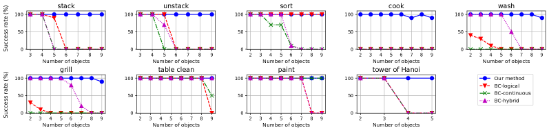
Figure 4: Comparison of the success rates of basic planning tasks for increasing numbers of objects to baselines.

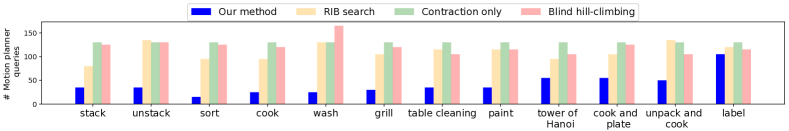
Figure 5: Comparison of the number of queries to motion planners during domain optimization to baselines.

IV-D Domain Optimization by Generate-and-Test Search

The domain optimization process is based on the generate-and-test search method, a heuristic search technique that involves backtracking [18]. Starting from $\mathbf{D_{\mathrm{top}}}$, the optimization process iterates through all possible domains until the domain successfully solves the validation problem set $\mathbf{Q}_{v}$ with the minimal number of predicates and actions. There are two assumptions made to perform the generate and test search:

Assumption 1.

If a domain $\mathbf{D}$ is incomplete, then any subdomain $\mathbf{D_{s}}\subseteq\mathbf{D}$ is incomplete.

Assumption 2.

If a domain $\mathbf{D}$ is complete, then the optimal domain $\mathbf{D_{\mathrm{optm}}}\subseteq\mathbf{D}$.

Algorithm 1 Domain Optimization Algorithm.

1:$\mathbf{D_{\mathrm{perturb}}}=\mathbf{D_{\mathrm{top}}}$ $\triangleright$ Initialization.

2:$is\_solved=plan(\mathbf{D_{\mathrm{perturb}}},\mathbf{Q}_{v})$

3:$element\_list=\omega_{\mathrm{\mathbf{D}}}^{\mathrm{top}}$

4:$\triangleright$ $top(\mathbf{\mathit{L}}$) returns the highest-scored element from $\mathbf{\mathit{L}}$.

5:while not $is\_solved$ do

6:     $\mathbf{D_{\mathrm{perturb}}}=add(\mathbf{D_{\mathrm{perturb}}},top(\mathbf{\mathit{L}}))$

7:     $is\_solved=plan(\mathbf{D_{\mathrm{perturb}}},\mathbf{Q}_{v})$

8:     $element\_list.insert(top(\mathbf{\mathit{L}}))$

9:     $\mathbf{\mathit{L}}.pop(top(\mathbf{\mathit{L}}))$

10:end while

11:$\mathbf{D_{\mathrm{optm}}}=\mathbf{D_{\mathrm{expanded}}}=\mathbf{D_{\mathrm{perturb}}}$

12:for $e_{i}\in element\_list$ do

13:     $\mathbf{D_{\mathrm{perturb}}}=remove(\mathbf{D_{\mathrm{optm}}},e_{i})$

14:     $is\_solved=plan(\mathbf{D_{\mathrm{perturb}}},\mathbf{Q}_{v})$

15:     if $is\_solved$ then

16:         $\mathbf{D_{\mathrm{optm}}}=\mathbf{D_{\mathrm{perturb}}}$

17:     end if

18:end for

The optimization process aims to add or remove predicates (actions) from the initial guess until the optimal domain is found. The domain $\mathbf{D_{\mathrm{perturb}}}$ is initialized as $\mathbf{D_{\mathrm{top}}}$. There are two major stages in the optimization process: expansion and contraction.

In the expansion stage, $\mathbf{D_{\mathrm{perturb}}}$ is expanded until it solves the validation problem set $\mathbf{Q}_{v}$. In each iteration, we move the top predicate(action) from priority list $\mathbf{\mathit{L}}$ and add it to $\mathbf{D_{\mathrm{perturb}}}$. The algorithm plans with $\mathbf{D_{\mathrm{perturb}}}$ to solve $\mathbf{Q}_{v}$. We continue expansion until $\mathbf{D_{\mathrm{perturb}}}$ can fully solve $\mathbf{Q}_{v}$.

In the contraction stage, we remove redundant elements from $\mathbf{D_{\mathrm{optm}}}$ until no more elements can be removed while maintaining domain completeness. The output domain from the expansion stage, $\mathbf{D_{\mathrm{expanded}}}$, is initialized as $\mathbf{D_{\mathrm{optm}}}$. In each iteration $i$, we remove one element (either a predicate or an action), $e_{i}\in\mathbf{D_{\mathrm{optm}}}$, to produce a perturbed domain $\mathbf{D_{\mathrm{perturb}}}$. If $\mathbf{D_{\mathrm{perturb}}}$ fully solves $\mathbf{Q}_{v}$, the removed element $e_{i}$ is redundant. Then $\mathbf{D_{\mathrm{perturb}}}$ becomes the new optimal domain $\mathbf{D_{\mathrm{optm}}}$. If $\mathbf{D_{\mathrm{perturb}}}$ fails to solve $\mathbf{Q}_{v}$, the removed element $e_{i}$ is critical. In this case, we backtrack to the last $\mathbf{D_{\mathrm{optm}}}$. This iteration continues until each element in $\mathbf{D_{\mathrm{expanded}}}$ has been evaluated.

V Experiments

In this section, we introduce the baselines and experimental tasks. Through our experiments, we aim to answer the following questions: (Q1) How effective is planning using the inferred planning domain? (Q2) Can we generalize to unseen and more complex tasks? (Q3) During the testing phase, how much does our method reduce computational costs in domain generation?

V-A Planning Baselines

We compared the planning success rate of our method to behavior cloning baselines to highlight its improved efficiency and generalizability. All baselines are trained per task type. The graph attention network training is implemented in PyTorch [24] and PyTorch Geometric [5].

BC-logical: Inspired by prior work [34], this baseline uses logical scene graphs to train a GAT task planning policy. The scene graph formulation is the same as that of our estimator. Using the current and goal logical scene graph as input, BC-logical outputs the next logical action to be executed.

BC-continuous: This baseline is a modification of BC-logical. However, the node features of the input scene graph nodes contain only continuous object states.

BC-hybrid: Inspired by recent papers combining continuous and logical data for imitation learning in TAMP [12, 15], BC-hybrid deviates from BC-logical by using both continuous and logical states of objects in the node features.

V-B Domain Optimization Baselines

We also compare our domain optimization method to a few baselines to evaluate how much our method reduces computational cost.

RIB search: The random-initial-and-blind (RIB) search method randomly samples an initial planning domain and searches through all possible planning domains blindly. This method terminates when the planning domain is complete and no predicates or actions can be further removed.

Contraction: This method deviates from the RIB search method as it starts with an initial planning domain that contains all predicates and actions in $\mathbf{P}$ and $\mathbf{A}$.

Blind hill-climbing: Inspired by the recent work in automatic planning domain generation [14, 28], this search method starts with an empty initial planning domain and searches through all possible planning domains via hill-climbing. This method searches for the planning domain with the highest planning success rate while maintaining the minimal planning domain size.

V-C Experimental Tasks

Experiments are developed on the PyBullet simulation [4]. The task planner is based on the PDDLStream library [7], and the motion planner is based on the pybullet-planning library [6]. We designed nine basic tasks and three composed tasks, including classic cube manipulation, everyday task scenarios, and puzzle solving, to evaluate our method.

Basic tasks: In stacking, the robot needs to stack cubes into a tower in a specific order. In the unstacking task, the objective is to disassemble the tower of cubes. In sorting, the robot needs to cluster cubes into two groups at different locations. In washing, the robot needs to wash food ingredients in the kitchen sink. In grilling, the robot needs to grill food on the stove. The cooking task involves a combination of washing and grilling food. The table cleaning task indicates collecting objects from the table and storing them in a bin. The painting task involves drawing random figures on an object or a piece of paper. The last basic task is to solve tower of Hanoi.

Composed tasks: Composed tasks are formed by combining multiple basic tasks. The unpack-and-cook task involves unstacking raw materials and cooking them. In cook-and-plate task, the robot needs to cook the raw materials and stack them together. The labeling task requires the robot to unstack piles of objects and then label each item with a pen.

V-D Training and Testing Dataset

The training dataset includes 30 demonstrations per basic task (no composed task), each involving a solvable TAMP problem containing two to four objects. For baseline training, the solution trajectory for each TAMP problem is formulated as state-action pairs. The test dataset includes 870 different TAMP problems, encompassing both basic and composed tasks, with object counts in the planning environment ranging from two to nine. For each object count, 10 test problems are generated with randomized object positions, and each problem must be solved within 30 seconds.

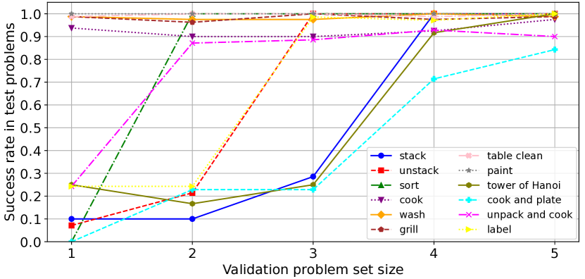
Figure 6: Planning success rate of the domain inferred with different sizes of validation problem set $\mathbf{Q}_{v}$ that assist domain optimization in Algorithm 1.

V-E Real Robot Experiments

To demonstrate the effectiveness of our system with real robots, we implemented two real-robot experiments: one involving the Tower of Hanoi and the other focusing on stacking multiple cube towers. We adopt NVIDIA’s FoundationPose [30] to capture visual demonstrations, which provides the 6D pose trajectories of all objects in the video. These poses are then consumed downstream to compute predicates concerning the objects in the scene. The real-robot validation problems are set up manually, with photos of the initial and goal configurations processed in the same way. The inferred planning domain is combined with the ROS Moveit motion planner and deployed on a Franka Research 3 arm.

Table I: Success rates for composed planning tasks.

Task Type	Number of Objects
		3	4	5	6	7	8	9
Cook and Plate		100	100	100	100	100	40	50
Unpack and Cook		100	100	100	100	100	80	50
Label		100	100	100	100	100	100	100

VI Results and Discussion

To address (Q1), we evaluate our method on various tasks and compare it to a few baselines. As illustrated in Figure 4, our method consistently outperforms the baselines in planning success rate across all basic tasks. While both our method and the baselines perform well on simpler tasks (painting, table cleaning, and sorting), the baselines degrade significantly on more complex tasks with larger decision spaces. To address (Q2), we evaluate our methods with planning problems that involve an increased number of objects, as well as unseen composed tasks. Figure 4 shows that our method maintains success rates above 90% even with up to nine objects, while the behavior cloning baseline method experiences a sharp decline as the number of objects increases. These results indicate that our method has a significant advantage in generalizing to a more complex experiment setup. Furthermore, as shown in Table I, our method demonstrates excellent planning performance on generalizing to unseen composed tasks. With just one human demonstration per task, our method successfully infers the planning domain, enabling efficient planning even when the number of objects increases and their positions are shuffled. Since we only have one trajectory per composed task, we did not compare our method with the baselines. Training a behavior cloning policy with just one trajectory would be trivial. To answer (Q3), we compare the computational cost of domain optimization to the baselines. The computational cost is assessed based on the number of queries made to the motion planner, which is the most time-intensive component of the optimization process. This metric is chosen because it provides a consistent comparison independent of the computer’s performance. As shown in Figure 5, our method drastically lowers the computational cost in the optimization process. The reduction in computational cost is more apparent for basic task types and attenuates when dealing with composed task types because the most relevant domain prediction becomes less accurate. Figure 6 shows our method’s testing planning success rate of the domain inferred with different sizes of the validation problem set $\mathbf{Q}_{v}$ via Algorithm 1. The results indicate that our method requires only a small $\mathbf{Q}_{v}$. For many tasks, the correct planning domain can be inferred with just one or two validation problems. Even in more challenging scenarios, five validation problems are sufficient. The real robot experiment, presented in Figure 7, demonstrates the effectiveness of our method on real robots. Remarkably, we only need to demonstrate once for the real robot to learn and solve similar TAMP problems.

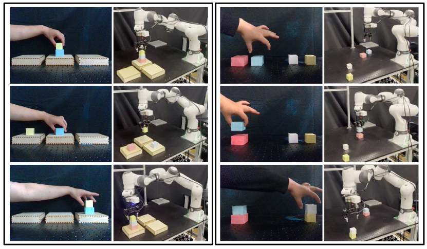
Figure 7: Real robot experiment. Left: Towers of Hanoi. Right: Stack multiple towers

VII Conclusion

This paper proposes a method for automatically inferring planning domains in task and motion planning by integrating deep learning and search. Our approach was evaluated in various planning environments, showing improved planning performance and generalizability compared to existing learning-based TAMP solvers. We also demonstrate a significant reduction in computational costs during domain optimization compared to common search algorithms. Real robot experiments are performed to validate the feasibility of deploying our method in a real-world implementation.

References

- [1] Rohan Chitnis et al. “Guided search for task and motion plans using learned heuristics” In 2016 IEEE International Conference on Robotics and Automation (ICRA), 2016, pp. 447–454 IEEE
- [2] Murtaza Dalal et al. “Imitating task and motion planning with visuomotor transformers” In arXiv preprint arXiv:2305.16309, 2023
- [3] Maximilian Diehl, Chris Paxton and Karinne Ramirez-Amaro “Automated generation of robotic planning domains from observations” In 2021 IEEE/RSJ International Conference on Intelligent Robots and Systems (IROS), 2021, pp. 6732–6738 IEEE
- [4] Benjamin Ellenberger “PyBullet Gymperium”, https://github.com/benelot/pybullet-gym, 2018–2019
- [5] Matthias Fey and Jan Eric Lenssen “Fast graph representation learning with PyTorch Geometric” In arXiv preprint arXiv:1903.02428, 2019
- [6] Caelan Reed Garrett, Tomás Lozano-Pérez and Leslie Pack Kaelbling “Backward-forward search for manipulation planning” In 2015 IEEE/RSJ International Conference on Intelligent Robots and Systems (IROS), 2015, pp. 6366–6373 IEEE
- [7] Caelan Reed Garrett et al. “Integrated task and motion planning” In Annual review of control, robotics, and autonomous systems 4.1 Annual Reviews, 2021, pp. 265–293
- [8] David González, Joshué Pérez, Vicente Milanés and Fawzi Nashashibi “A review of motion planning techniques for automated vehicles” In IEEE Transactions on intelligent transportation systems 17.4 IEEE, 2015, pp. 1135–1145
- [9] Yuqian Jiang, Fangkai Yang, Shiqi Zhang and Peter Stone “Task-motion planning with reinforcement learning for adaptable mobile service robots” In 2019 IEEE/RSJ International Conference on Intelligent Robots and Systems (IROS), 2019, pp. 7529–7534 IEEE
- [10] Kei Kase et al. “Transferable task execution from pixels through deep planning domain learning” In 2020 IEEE International Conference on Robotics and Automation (ICRA), 2020, pp. 10459–10465 IEEE
- [11] Mohamed Khodeir, Ben Agro and Florian Shkurti “Learning to search in task and motion planning with streams” In IEEE Robotics and Automation Letters 8.4 IEEE, 2023, pp. 1983–1990
- [12] Mohamed Khodeir, Atharv Sonwane, Ruthrash Hari and Florian Shkurti “Policy-guided lazy search with feedback for task and motion planning” In 2023 IEEE International Conference on Robotics and Automation (ICRA), 2023, pp. 3743–3749 IEEE
- [13] Beomjoon Kim and Luke Shimanuki “Learning value functions with relational state representations for guiding task-and-motion planning” In Conference on robot learning, 2020, pp. 955–968 PMLR
- [14] Nishanth Kumar et al. “Learning efficient abstract planning models that choose what to predict” In Conference on Robot Learning, 2023, pp. 2070–2095 PMLR
- [15] Yixin Lin, Austin S Wang, Eric Undersander and Akshara Rai “Efficient and interpretable robot manipulation with graph neural networks” In IEEE Robotics and Automation Letters 7.2 IEEE, 2022, pp. 2740–2747
- [16] Li Liu, Fu Guo, Zishuai Zou and Vincent G Duffy “Application, development and future opportunities of collaborative robots (cobots) in manufacturing: A literature review” In International Journal of Human–Computer Interaction 40.4 Taylor & Francis, 2024, pp. 915–932
- [17] Tomás Lozano-Pérez and Michael A Wesley “An algorithm for planning collision-free paths among polyhedral obstacles” In Communications of the ACM 22.10 ACM New York, NY, USA, 1979, pp. 560–570
- [18] Ashique Rupam Mahmood and Richard S Sutton “Representation search through generate and test” In Workshops at the Twenty-Seventh AAAI conference on artificial intelligence, 2013
- [19] Drew McDermott et al. “PDDL-the planning domain definition language”, 1998 URL: https://api.semanticscholar.org/CorpusID:59656859
- [20] Michael James McDonald and Dylan Hadfield-Menell “Guided imitation of task and motion planning” In Conference on Robot Learning, 2022, pp. 630–640 PMLR
- [21] MG Mohanan and Ambuja Salgoankar “A survey of robotic motion planning in dynamic environments” In Robotics and Autonomous Systems 100 Elsevier, 2018, pp. 171–185
- [22] Shohin Mukherjee et al. “Reactive long horizon task execution via visual skill and precondition models” In 2021 IEEE/RSJ International Conference on Intelligent Robots and Systems (IROS), 2021, pp. 5717–5724 IEEE
- [23] Brian Paden et al. “A survey of motion planning and control techniques for self-driving urban vehicles” In IEEE Transactions on intelligent vehicles 1.1 IEEE, 2016, pp. 33–55
- [24] Adam Paszke et al. “Automatic differentiation in pytorch”, 2017
- [25] Chris Paxton, Vasumathi Raman, Gregory D Hager and Marin Kobilarov “Combining neural networks and tree search for task and motion planning in challenging environments” In 2017 IEEE/RSJ International Conference on Intelligent Robots and Systems (IROS), 2017, pp. 6059–6066 IEEE
- [26] Jacob T. Schwartz and Micha Sharir “A survey of motion planning and related geometric algorithms” In Artificial Intelligence 37.1-3 Elsevier, 1988, pp. 157–169
- [27] Tom Silver et al. “Planning with learned object importance in large problem instances using graph neural networks” In Proceedings of the AAAI conference on artificial intelligence 35.13, 2021, pp. 11962–11971
- [28] Tom Silver et al. “Predicate invention for bilevel planning” In Proceedings of the AAAI Conference on Artificial Intelligence 37.10, 2023, pp. 12120–12129
- [29] Xu Wang et al. “Deep reinforcement learning: A survey” In IEEE Transactions on Neural Networks and Learning Systems 35.4 IEEE, 2022, pp. 5064–5078
- [30] Bowen Wen, Wei Yang, Jan Kautz and Stan Birchfield “FoundationPose: Unified 6D Pose Estimation and Tracking of Novel Objects” In Proceedings of the IEEE/CVF Conference on Computer Vision and Pattern Recognition (CVPR), 2024, pp. 17868–17879
- [31] Danfei Xu et al. “Deep affordance foresight: Planning through what can be done in the future” In 2021 IEEE international conference on robotics and automation (ICRA), 2021, pp. 6206–6213 IEEE
- [32] Zhutian Yang et al. “Sequence-based plan feasibility prediction for efficient task and motion planning” In arXiv preprint arXiv:2211.01576, 2022
- [33] Chengmin Zhou, Bingding Huang and Pasi Fränti “A review of motion planning algorithms for intelligent robots” In Journal of Intelligent Manufacturing 33.2 Springer, 2022, pp. 387–424
- [34] Yifeng Zhu, Jonathan Tremblay, Stan Birchfield and Yuke Zhu “Hierarchical planning for long-horizon manipulation with geometric and symbolic scene graphs” In 2021 IEEE International Conference on Robotics and Automation (ICRA), 2021, pp. 6541–6548 IEEE