Discriminating image representations with
principal distortions

Abstract

Image representations (artificial or biological) are often compared in terms of their global geometry; however, representations with similar global structure can have strikingly different local geometries. Here, we propose a framework for comparing a set of image representations in terms of their local geometries. We quantify the local geometry of a representation using the Fisher information matrix, a standard statistical tool for characterizing the sensitivity to local stimulus distortions, and use this as a substrate for a metric on the local geometry in the vicinity of a base image. This metric may then be used to optimally differentiate a set of models, by finding a pair of “principal distortions” that maximize the variance of the models under this metric. We use this framework to compare a set of simple models of the early visual system, identifying a novel set of image distortions that allow immediate comparison of the models by visual inspection. In a second example, we apply our method to a set of deep neural network models and reveal differences in the local geometry that arise due to architecture and training types. These examples highlight how our framework can be used to probe for informative differences in local sensitivities between complex computational models, and suggest how it could be used to compare model representations with human perception.

1 Introduction

Biological and artificial neural networks transform sensory stimuli into high-dimensional internal representations that support downstream tasks, and these representations are often described in terms of their neural population geometry (Chung & Abbott, 2021). This idea has led to a multitude of proposed measures of representational similarity (Kriegeskorte et al., 2008; Yamins & DiCarlo, 2016; Kornblith et al., 2019; Williams et al., 2021; Klabunde et al., 2023), and these measures are often used to compare representations within a computational model to the representations within a brain. However, despite differing in architectures and training procedures, many computational models of perceptual or neural responses are equally performant on these representational similarity measures (Schrimpf et al., 2018; Tuckute et al., 2023; Conwell et al., 2022). Are these models functionally interchangeable, or are the datasets and methods that are used to test them simply insufficient to reveal their differences?

Often the similarity between two representations is quantified by measuring alignment of the representations over a set of natural stimuli that are relatively far apart in stimulus space. In this way, these measures capture notions of global geometric similarity between representations. However, systems with similar global structure can have strikingly different local geometries. For example, Szegedy et al. (2013) found image distortions that were imperceptible to humans but led artificial neural networks to misclassify images, which motivated methods for training artificial neural networks so as to minimize their susceptibility to these adversarial examples (Goodfellow et al., 2014; Madry, 2017). These observations suggest a need for metrics that compare the local geometries of image representations and, in particular, highlight the differences between systems even when global structure seems similar.

How can we quantify and compare the local geometry of different image representations? A brute-force comparison clearly is prohibitive: the space of images is extremely high-dimensional, and the set of potential distortions equally high-dimensional. Estimating the local geometry of representations over a moderately dense sampling of this full set of possible distortions is impractical, and estimating human sensitivity to such a set is essentially impossible. As such, it is worthwhile to develop a method for judicious selection of stimulus distortions that can be used when comparing a set of models.

We take inspiration from Zhou et al. (2023). For a pair of models and a base image, they synthesize distortions along which the two models’ sensitivities maximally disagree. This bears conceptual similarity to other methods that construct stimuli to optimally distinguish a pair of models (Wang & Simoncelli, 2008; Golan et al., 2020) or cluster neurons by cell type (Burg et al., 2024), and builds on earlier work that examined “eigen-distortions” along which individual models are maximally/minimally sensitive (Berardino et al., 2017). Specifically, Zhou et al. measure the local sensitivity of a model in terms of its Fisher Information matrix (FIM, Fisher, 1925), a classical tool from statistical estimation theory, and choose the pair of “generalized eigen-distortions” that maximize/minimize the ratio of the two models’ sensitivities. Once these image distortions have been computed, they may be added in varying amounts to a base image to determine the level at which they become visible to a human. These measured human sensitivities can then be compared to those of the models, with the goal of identifying which model is better aligned with the local geometry of the human visual system. However, there is no principled method for selecting image distortions for use in comparing more than two models.

Here we define a novel metric for comparing model representations in terms of their relative sensitivities to image distortions. We then use this metric to generate a pair of distortions that maximize the variance across two or more models under this metric. In analogy with principal component analysis, our method can be viewed as a dimensionality reduction technique that preserves as much of the variability in the local representational geometry as possible. As such, we refer to these as the “principal distortions” of the set of models.

We apply our method to a nested set of hand-crafted models of the early visual system to identify distortions that differentiate these models and can potentially be used to evaluate how well these models predict human visual sensitivities. We then apply our method to a set of visual deep neural networks (DNNs) with varying architectures and training procedures. We find distortions that allow for visualization of differences in the sensitivities between layers of the networks and neural network architectures. We further explore differences between standard ImageNet trained networks and their shape-bias enhanced counterparts, and between standard networks and their adversarially-trained counterparts. In all cases, we illustrate how the method generates novel distortions that highlight differences between models.

Portions of this work were initially presented in (Lipshutz et al., 2024).

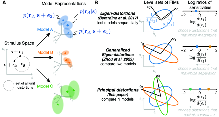
Figure 1: Comparing the local geometry of image representations. A) Each model maps stimuli to stochastic responses in a model’s representation space—biological neurons are inherently noisy, while a putatively deterministic model can be made stochastic by assuming additive Gaussian response noise. For example, Model A maps the stimulus ${\mathbf{s}}$ (solid black circle $\bullet$) to a conditional density $p({\mathbf{r}}_{A}|{\mathbf{s}})$ on Model A’s representation space (the solid blue circle $\bullet$ and surrounding transparent blue ellipse represent the mean and covariance of ${\mathbf{r}}_{A}$ conditioned on ${\mathbf{s}}$). B) A model’s sensitivity at the base image ${\mathbf{s}}$ to local distortions can be mapped back to the stimulus domain via the model’s positive semidefinite FIM. In the top panel “Eigen-distortions (Berardino et al., 2017)”, the blue ellipse represents the unit level set $\{{\bm{v}}:d_{A}({\bm{v}})=1\}$ of the norm induced by Model A’s FIM ${\bm{I}}_{A}$, which is the set of distortions of the base stimulus ${\mathbf{s}}$ that appear equally distorted according to Model A’s representation. The eigenvectors of the FIM (${\bm{\epsilon}}_{1}$, ${\bm{\epsilon}}_{2}$) can equivalently be interpreted as the distortions that maximize the magnitude of the log ratio of the model’s sensitivities, which is represented as a solid blue circle $\bullet$ on the number line. In the middle panel “Generalized Eigen-distortions (Zhou et al., 2023)”, the blue ellipse is copied from the top panel and the orange ellipse is the level set of Model B’s FIM ${\bm{I}}_{B}$. The generalized eigenvectors of ${\bm{I}}_{A}$ and ${\bm{I}}_{B}$ (${\bm{\epsilon}}_{1}$, ${\bm{\epsilon}}_{2}$) can equivalently be interpreted as the vectors that maximize the difference between the log ratios of the models’ sensitivities. In the bottom panel “Principal distortions (this paper)”, the blue and orange ellipses are as in the above panels and the green ellipse represents the level set of Model C’s FIM ${\bm{I}}_{C}$. We propose a general method for comparing an arbitrary number of models, by selecting two stimulus distortions (${\bm{\epsilon}}_{1}$, ${\bm{\epsilon}}_{2}$) that maximize the variance of the log ratios of model sensitivities.

2 Problem statement and existing methods

Given a collection of image representations, our goal is to develop a method for comparing the local geometries of these representations in the vicinity of some base input image. In this section, we define the local geometry of an image representation in terms of the FIM and review existing methods for selecting image distortions based on model FIMs.

2.1 Local information geometry of stochastic image representations

We assume that each image representation has an associated conditional density $p({\mathbf{r}}|{\mathbf{s}})$, where ${\mathbf{s}}$ is a $K$-dimensional vector of image pixels and ${\mathbf{r}}$ is a vector of stochastic responses (e.g., biological neuronal firing rates or deterministic neural network activations with additive response noise). Figure 1A depicts a two-dimensional stimulus space and three models mapping stimuli ${\mathbf{s}}$, ${\mathbf{s}}+{\bm{\epsilon}}_{1}$, and ${\mathbf{s}}+{\bm{\epsilon}}_{2}$ to conditional densities. Note that the dimension of the responses may vary across representations.

The sensitivity of the representation to a small distortion ${\bm{\epsilon}}$ depends on the overlap between the conditional distributions $p({\mathbf{r}}|{\mathbf{s}})$ and $p({\mathbf{r}}|{\mathbf{s}}+{\bm{\epsilon}})$, with less overlap corresponding to higher sensitivity (Green & Swets, 1966). This sensitivity can be precisely quantified in terms of the Fisher-Rao metric (Rao, 1945; Amari, 2016), a Riemannian metric on the stimulus space (Fig. 1B) that is defined in terms of the positive semi-definite FIM (Fisher, 1925):

$${\bm{I}}({\mathbf{s}}):=\mathbb{E}_{{\mathbf{r}}\sim p({\mathbf{r}}|{\mathbf{s}})}\left[\nabla_{{\mathbf{s}}}\log p({\mathbf{r}}|{\mathbf{s}})\nabla_{{\mathbf{s}}}\log p({\mathbf{r}}|{\mathbf{s}})^{\top}\right],$$

where $\nabla_{\mathbf{s}}\log p({\mathbf{r}}|{\mathbf{s}})$ denotes the gradient of $\log p({\mathbf{r}}|{\mathbf{s}})$ with respect to ${\mathbf{s}}$. The FIM is a standard tool in statistical estimation theory that locally approximates the expected log likelihood ratio (or KL divergence) between the conditional distributions $p({\mathbf{r}}|{\mathbf{s}})$ and $p({\mathbf{r}}|{\mathbf{s}}+{\bm{\epsilon}})$, and provides a lower bound on the variance of any unbiased estimator of ${\mathbf{s}}$ (Cramér, 1946; Rao, 1945). The FIM has also been used to link neural representations to perceptual discrimination (Paradiso, 1988; Seung & Sompolinsky, 1993; Brunel & Nadal, 1998; Averbeck & Lee, 2006; Seriès et al., 2009; Ganguli & Simoncelli, 2014; Wei & Stocker, 2016). Given the FIM, we can define the sensitivity of the representation of stimulus ${\mathbf{s}}$ to a distortion ${\bm{\epsilon}}$ as:

$$d({\mathbf{s}};{\bm{\epsilon}}):=\sqrt{{\bm{\epsilon}}^{\top}{\bm{I}}({\mathbf{s}}){\bm{\epsilon}}},$$ (1)

which quantifies how well an ideal observer could detect small perturbations of the base stimulus in the direction ${\bm{\epsilon}}$.

As a tractable example, suppose that the conditional response ${\mathbf{r}}$ is Gaussian with stimulus-dependent mean ${\bm{f}}({\mathbf{s}})$ and constant covariance ${\bm{\Sigma}}$. Then the FIM at ${\mathbf{s}}$ is

$${\bm{I}}({\mathbf{s}})={\bm{J}}_{f}({\mathbf{s}})^{\top}{\bm{\Sigma}}^{-1}{\bm{J}}_{f}({\mathbf{s}}),$$

where ${\bm{J}}_{f}({\mathbf{s}})$ is the Jacobian of ${\bm{f}}(\cdot)$ at ${\mathbf{s}}$. From this expression, we see that the sensitivities of a representation to a distortion ${\bm{\epsilon}}$ depend on how the mean response is changing in the direction ${\bm{\epsilon}}$ relative to the noise covariance.

2.2 Eigen-distortions of an image representation

Given a model image representation, Berardino et al. (2017) proposed the use of extremal eigenvectors of the model FIM (termed “eigen-distortions”, Fig. 1B, top panel) as model predictions of the most- and least-noticeable image distortions. For a set of early vision models and deep neural networks whose parameters were optimized to match a database of human image quality ratings (Ponomarenko et al., 2009), they computed the eigen-distortions of each model. Despite the fact that these models all fit the image quality data equally well, their eigen-distortions were quite different, and human perceptual judgements of the severity of these eigen-distortions varied substantially. The eigen-distortions of each image representation correspond to its most distinct distortion predictions, which can then be tested with human perceptual experiments. However, if the eigen-distortions of two models are similar, they will not be useful in distinguishing the models, since this method is insensitive to differences in the non-extremal eigenvectors.

2.3 Generalized eigen-distortions for comparing two image representations

Zhou et al. (2023) proposed comparing two image representations $A$ and $B$ along distortions in which their local sensitivities maximally differ, which is conceptually similar to previous methods that construct stimuli that maximize disagreement between models (Wang & Simoncelli, 2008; Golan et al., 2020). Specifically, they chose distortions to extremize the generalized Rayleigh quotient:

$${\bm{\epsilon}}_{1}({\mathbf{s}}) =\operatorname*{arg\,max}_{\bm{\epsilon}}\frac{{\bm{\epsilon}}^{\top}{\bm{I}}_{A}({\mathbf{s}}){\bm{\epsilon}}}{{\bm{\epsilon}}^{\top}{\bm{I}}_{B}({\mathbf{s}}){\bm{\epsilon}}}, {\bm{\epsilon}}_{2}({\mathbf{s}})=\operatorname*{arg\,min}_{\bm{\epsilon}}\frac{{\bm{\epsilon}}^{\top}{\bm{I}}_{A}({\mathbf{s}}){\bm{\epsilon}}}{{\bm{\epsilon}}^{\top}{\bm{I}}_{B}({\mathbf{s}}){\bm{\epsilon}}}.$$ (2)

Since these distortions correspond to the extremal eigenvectors of the generalized eigenvalue problem ${\bm{I}}_{A}({\mathbf{s}}){\bm{\epsilon}}=\lambda{\bm{I}}_{B}({\mathbf{s}}){\bm{\epsilon}}$, we refer to them as “generalized eigen-distortions” (Fig. 1B, middle panel). However, this method is limited to comparisons of pairs of models, or of a single model against the average of other models.

3 Principal distortions of image representations

We propose a natural extension of generalized eigen-distortions that allows for comparisons among more than two image representations. We show that the generalized eigenvalue problem suggests a metric on image representations, which can be used to optimally choose image distortions that distinguish more than two models.

3.1 A metric on the local geometry of image representations

We can re-express the generalized eigen-distortions defined in Equation 2 as the solutions of a single optimization problem:

$$\{{\bm{\epsilon}}_{1},{\bm{\epsilon}}_{2}\}=\operatorname*{arg\,max}_{{\bm{\epsilon}},{\bm{\epsilon}}^{\prime}}\left\{\log\frac{{\bm{\epsilon}}^{\top}{\bm{I}}_{A}{\bm{\epsilon}}}{{\bm{\epsilon}}^{\top}{\bm{I}}_{B}{\bm{\epsilon}}}-\log\frac{{\bm{\epsilon}}^{\prime\top}{\bm{I}}_{A}{\bm{\epsilon}}^{\prime}}{{\bm{\epsilon}}^{\prime\top}{\bm{I}}_{B}{\bm{\epsilon}}^{\prime}}\right\},$$

where we’ve simplified notation by omitting the dependence of ${\bm{I}}_{*}$ and ${\bm{\epsilon}}_{*}$ on ${\mathbf{s}}$. We can regroup the numerators and denominators of the log quotients by model rather than by distortion, to re-express the optimization problem as follows:

$$\{{\bm{\epsilon}}_{1},{\bm{\epsilon}}_{2}\}=\operatorname*{arg\,max}_{{\bm{\epsilon}},{\bm{\epsilon}}^{\prime}}m_{{\bm{\epsilon}},{\bm{\epsilon}}^{\prime}}({\bm{I}}_{A},{\bm{I}}_{B}),$$

where

$$m_{{\bm{\epsilon}},{\bm{\epsilon}}^{\prime}}({\bm{I}}_{A},{\bm{I}}_{B}):=\left|\log\frac{d_{A}({\bm{\epsilon}})}{d_{A}({\bm{\epsilon}}^{\prime})}-\log\frac{d_{B}({\bm{\epsilon}})}{d_{B}({\bm{\epsilon}}^{\prime})}\right|$$ (3)

and we have used the definition of the sensitivity in Equation 1 and dropped a factor of 2. For any pair of distortions ${\bm{\epsilon}},{\bm{\epsilon}}^{\prime}$, the function $m_{{\bm{\epsilon}},{\bm{\epsilon}}^{\prime}}(\cdot,\cdot)$ is a proper metric on positive semi-definite matrices. Specifically, it is non-negative, symmetric, obeys the triangle inequality, and is zero when ${\bm{I}}_{A}={\bm{I}}_{B}$. This metric has several appealing properties:

• Invariance to scaling of the FIMs by positive constants $c_{A},c_{B}>0$:

  $$m_{{\bm{\epsilon}},{\bm{\epsilon}}^{\prime}}({\bm{I}}_{A},{\bm{I}}_{B})=m_{{\bm{\epsilon}},{\bm{\epsilon}}^{\prime}}(c_{A}{\bm{I}}_{A},c_{B}{\bm{I}}_{B}).$$

  This is a desirable property since we are interested in identifying relevant image distortions that depend on the shape of the FIMs, independent of scaling factors.

• Invariance to permutation of the distortions ${\bm{\epsilon}}$ and ${\bm{\epsilon}}^{\prime}$:

  $$m_{{\bm{\epsilon}},{\bm{\epsilon}}^{\prime}}({\bm{I}}_{A},{\bm{I}}_{B})=m_{{\bm{\epsilon}}^{\prime},{\bm{\epsilon}}}({\bm{I}}_{A},{\bm{I}}_{B}).$$

• When ${\bm{\epsilon}}_{1}$ and ${\bm{\epsilon}}_{2}$ are the generalized eigen-distortions of ${\bm{I}}_{A}$ and ${\bm{I}}_{B}$, $m_{{\bm{\epsilon}}_{1},{\bm{\epsilon}}_{2}}({\bm{I}}_{A},{\bm{I}}_{B})$ is an approximation of the Fisher-Rao distance between mean-zero Gaussian distributions with covariances ${\bm{I}}_{A}$ and ${\bm{I}}_{B}$ (up to scaling factors, see Appx. A). This interpretation suggests a principled extension of the metric to more than two distortions.

• The metric compares stochastic representations back in stimulus space via their FIMs. This avoids the problem of aligning the stochastic representations, which is a computationally intensive step that is required when evaluating existing metrics on stochastic representations (Duong et al., 2023b).

3.2 Principal distortions for comparing multiple image representations

To optimize a pair of image distortions for distinguishing $N>2$ representations, $A_{1},\dots,A_{N}$, we choose ${\bm{\epsilon}}_{1},{\bm{\epsilon}}_{2}$ to maximize the sum of the squares of all pairwise distances between the FIMs under the metric defined in Equation 3:

$$\{{\bm{\epsilon}}_{1},{\bm{\epsilon}}_{2}\}=\operatorname*{arg\,max}_{{\bm{\epsilon}},{\bm{\epsilon}}^{\prime}}\sum_{n=1}^{N}\sum_{m=1}^{N}m_{{\bm{\epsilon}},{\bm{\epsilon}}^{\prime}}^{2}({\bm{I}}_{A_{n}},{\bm{I}}_{A_{m}}).$$ (4)

This is equivalent to maximizing the variance of the image representations’ log sensitivity ratios:

$$\{{\bm{\epsilon}}_{1},{\bm{\epsilon}}_{2}\}=\operatorname*{arg\,max}_{{\bm{\epsilon}},{\bm{\epsilon}}^{\prime}}\sum_{n=1}^{N}\left|\log\frac{d_{A_{n}}({\bm{\epsilon}})}{d_{A_{n}}({\bm{\epsilon}}^{\prime})}-\frac{1}{N}\sum_{m=1}^{N}\log\frac{d_{A_{m}}({\bm{\epsilon}})}{d_{A_{m}}({\bm{\epsilon}}^{\prime})}\right|^{2}$$

We refer to $\{{\bm{\epsilon}}_{1},{\bm{\epsilon}}_{2}\}$ as the “principal distortions” of the models, analogous to principal component analysis (Fig. 1B). For a gradient-based optimization algorithm, see Appx. B.

Note that there are several other natural extensions of generalized-eigendistortions when considering $N>2$ models. For example, for any $p\geq 1$, one can choose distortions ${\bm{\epsilon}}_{1},{\bm{\epsilon}}_{2}$ that maximize the sum of the $p$^th power of all pairwise distances, which amounts to replacing $m_{{\bm{\epsilon}},{\bm{\epsilon}}^{\prime}}^{2}({\bm{I}}_{A_{n}},{\bm{I}}_{A_{m}})$ in Equation 4 with $m_{{\bm{\epsilon}},{\bm{\epsilon}}^{\prime}}^{p}({\bm{I}}_{A_{n}},{\bm{I}}_{A_{m}})$. Here we focus on the case of maximizing the variance ($p=2$) and leave an exploration of higher-order moments to future work

4 Experimental results

As a demonstration of our method, we generated principal distortions for computational models previously proposed to capture aspects of the human visual system. All models were implemented in PyTorch (Ansel et al., 2024) and simulations were performed on NVIDIA GPUs (RTX A6000 and A100 models). As the models are deterministic, we calculate the FIM by assuming the network output is corrupted by additive Gaussian noise, as in (Berardino et al., 2017). In this case, ${\bm{I}}({\mathbf{s}})={\bm{J}}_{f}({\mathbf{s}})^{\top}{\bm{J}}_{f}({\mathbf{s}})$, where ${\bm{J}}_{f}({\mathbf{s}})$ is the Jacobian of the model ${\bm{f}}(\cdot)$ at input ${\mathbf{s}}$.

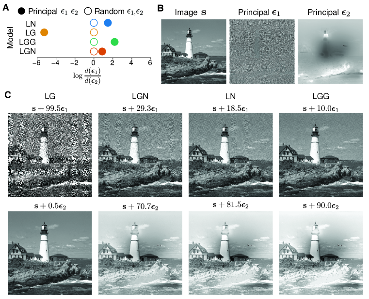
Figure 2: Principal distortions of a set of early visual models. A) Log sensitivity ratios of the two principal distortions and two random distortions for each of the four models (Berardino et al., 2017). Models in nested order (LN is the most basic, LGN is the full model). Principal distortions (filled circles) separate the log ratios, while random distortions (hollow circles) do not. B) Natural image $\mathbf{s}$ and corresponding optimized principal distortions $\{{\bm{\epsilon}}_{1},{\bm{\epsilon}}_{2}\}$. C) Natural image corrupted by principal distortions, with each pair scaled so as to be equally detectable by the corresponding model (abbreviations above). Models are ordered by the log ratio of their sensitivities (panel A). If a model’s thresholds are comparable to human thresholds, the two scaled distortions should be equally visible in the top and bottom images. Note: Distorted images are best viewed at high resolution.

4.1 Early visual models

We generated principal distortions for a nested family of models designed to capture the response properties of early stages (specifically, the lateral geneiculate nucleus, LGN) of the primate visual system (Fig. 2). The full model (LGN) contains two parallel cascades representing ON and OFF center-surround filter channels, rectification, and both luminance and contrast gain control nonlinearities. The other models are reduced versions of this model. LGG removes the OFF channel, LG additionally removes the contrast gain control, and LN removes both gain control operations. The filter sizes, amplitudes, and normalization values of each model were previously fit separately to predict a dataset of human distortion ratings (Berardino et al., 2017, see details in Appx. C).

As these models were explicitly trained to predict human distortion thresholds, we provide a qualitative comparison of each model’s sensitivities to human distortion sensitivity (Fig. 2C). We adjusted the relative scaling of the principal distortion so as to be equally detectable by that model while constraining the sum of the Euclidean norms of the two distortions to be a fixed value of 100; that is, we chose positive scalars $c_{1},c_{2}$ such that $d(c_{1}{\bm{\epsilon}}_{1})=d(c_{2}{\bm{\epsilon}}_{2})$ and $c_{1}+c_{2}=100$. If a model’s thresholds are comparable to human thresholds, then these rescaled distortions should be equally detectable when added to the image ${\mathbf{s}}$. Visual inspection of these images reveals that both distortions are visible when rescaled for the LGN model and the LN model, suggesting that these models are closest to human distortion thresholds. For LG, the scaled ${\bm{\epsilon}}_{2}$ distortion is not visible, while the scaled ${\bm{\epsilon}}_{1}$ distortion is immediately apparent, suggesting a strong mismatch with human observer thresholds. The same is true of the LGG model, with the roles of the two distortions swapped. These qualitative observations are consistent with the results of (Berardino et al., 2017), in which experiments on eigen-distortions suggested that the LGN model was the best of these models in terms of consistency with human distortion sensitivity. Analogous perceptual experiments could be used to quantify the visibility of the principal distortions arising from our analysis.

An advantage of our framework is that it can dramatically reduce the number of distortions that are needed to differentiate a set of models. For instance, to judge how well these models of the early visual system capture human perceptual discrimination thresholds, Berardino et al. (2017) computed the extremal eigen-distortions for each of the four models, and then measured human perceptual discrimination thresholds to all eight distortions. In general, their method requires assessing visibility of $2N$ distortions, for $N$ models. Zhou et al. (2023) considered a pair of generalized eigen-distortions for each pair of models, for a total of $N(N+1)$ distortions. In contrast, our method always selects the two distortions that maximize the variance across the models, independent of $N$. Human sensitivities to these distortions can then be estimated in perceptual discrimination experiments to judge which model(s) are closest in terms of the metric we defined Equation 3. The models whose sensitivities are far from human sensitivities can be discarded and this procedure can be repeated to best differentiate the remaining models, and so on. If one could reduce the number of models by, say, a factor of two on each iteration of this process, the total number of stimuli to be assessed scales as $2\log_{2}(N)$. This dramatic improvement in efficiency could enable the comparison of significantly larger sets of models than feasible with previous methods.

4.2 Deep neural networks

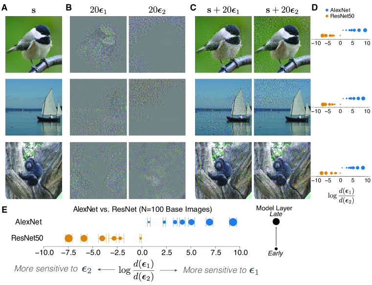
Figure 3: AlexNet versus ResNet50. A) Example base images. B) Optimized principal distortions (scaled by a factor of 20 for visibility, and using the convention $\|{\bm{\epsilon}}\|=1$ here and in other figures). C) Base image plus principal distortions. D) Log sensitivity ratios of principal distortions when comparing image representations at multiple layers of in AlexNet and ResNet50. Assignment of ${\bm{\epsilon}}_{1}$ and ${\bm{\epsilon}}_{2}$ was chosen so that the final tested layer of AlexNet has a positive log ratio. E) Log sensitivity ratios averaged across 100 base images (error bars are standard deviation). The principal distortions organize the networks by architecture—the log sensitivity ratios of AlexNet and ResNet50 are separated and early layers have smaller log ratios than late layers. AlexNet is more sensitive to distortion ${\bm{\epsilon}}_{1}$, which is concentrated on higher contrast or textured parts of the image (often the foreground object). ResNet50 is more sensitive to distortion ${\bm{\epsilon}}_{2}$ which concentrates power on relatively smooth parts of the image, such as regions of constant intensity/color.

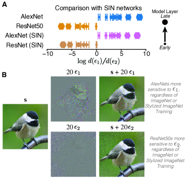
Figure 4: Comparison of AlexNet and ResNet50 variants trained to increase “Shape Bias” of networks. A) Log sensitivity ratios of principal distortions for networks trained on standard ImageNet and Stylized ImageNet (SIN). Average log sensitivity is computed across 100 base images (error bars are standard deviation) and the choice of ${\bm{\epsilon}}_{1}$ is set such that $d({\bm{\epsilon}}_{1})\geq 0$ for the last tested layer of the standard AlexNet. B) Example base image and the optimized principal distortions. Similar to the analysis of the ImageNet-trained ResNet50 and AlexNet (Fig. 3), ${\bm{\epsilon}}_{1}$ is concentrated on parts of the image with higher spatial frequencies while ${\bm{\epsilon}}_{2}$ is concentrated on parts of the image with relatively solid patches. Both AlexNet architectures are more sensitive to ${\bm{\epsilon}}_{1}$ while both ResNet50 architectures are more sensitive to ${\bm{\epsilon}}_{2}$, suggesting that the differences in local sensitivities of these networks depend more on differences in architecture than training procedure.

Deep Neural Networks (DNNs), originally developed for object recognition, have also been examined as models of the primate visual system (Yamins & DiCarlo, 2016; Schrimpf et al., 2018; Lindsay, 2021). A plethora of models, varying in architecture and training techniques, have been proposed, but many of these models perform quite similarly on behavioral tasks or neural benchmarks (Schrimpf et al., 2018; Tuckute et al., 2023; Conwell et al., 2022). This situation offers a well-aligned opportunity for use of our principal distortion method.

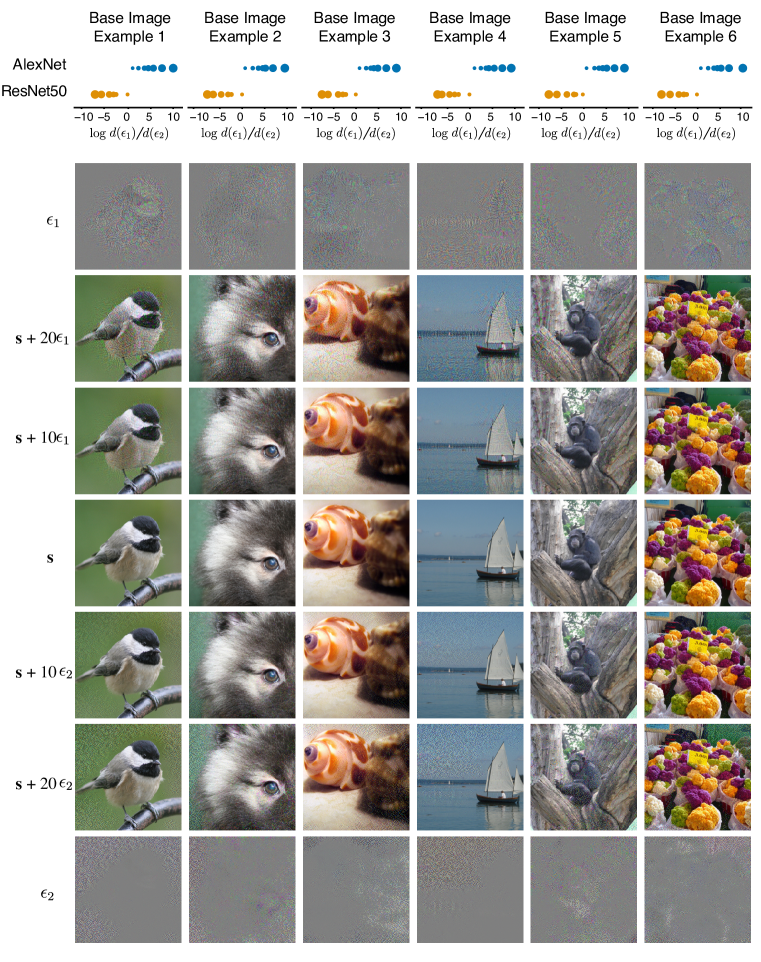
Figure 6: Principal distortions for ResNet50 and AlexNet for six example base images (${\mathbf{s}}$, middle row). Each row shows base images with differently scaled additive perturbations of ${\bm{\epsilon}}_{1}$ and ${\bm{\epsilon}}_{2}$. Distortions $\{{\bm{\epsilon}}_{1},{\bm{\epsilon}}_{2}\}$ are shown in isolation in the top/bottom rows, respectively. The log ratio plot for each image is at the top of the column.

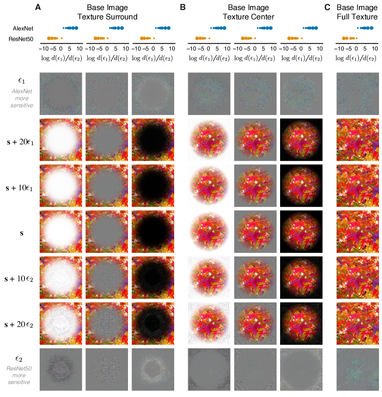
Figure 7: Principal distortions for ResNet50 and AlexNet for base images that have been constructed to have either (A) texture only in the periphery and a blank center (B) texture only in the center and a blank surround and (C) a full image of texture. The log ratio plot for each image is at the top of the column. Panels A and B highlight that the AlexNet architecture is more sensitive to the perturbation with power around the “stuff” of the image (i.e., the non-blank areas), while ResNet50 is more sensitive to a distortion focused on blank areas of the image, and these perturbations are not sensitive to the choice of low contrast (“black”) or high luminance (“white”) for the blank part of the space. Panel C highlights that in the case where there is not obvious blank area of the image, the perturbations become harder to interpret, and this reflects the locally adaptive property of the FI to the input image.

We first measured the FIM of a set of layers from two different architectures trained on the ImageNet object classification task—AlexNet (Krizhevsky et al., 2012) and ResNet50 (He et al., 2016)—and generated the principal distortions that maximally separate these models (Fig. 3, see Sec. D of the supplement for layer choices and model details). Although these architectures are not currently state-of-the-art at image recognition or neural prediction, they have been widely used and trained with various optimization strategies. Notably, the hierarchical structure of the models is reflected in the log ratios of the sensitivities, where early layers of the models are closer together in the metric space (Fig. 3D), and late layers of AlexNet are always more sensitive to ${\bm{\epsilon}}_{1}$ when late layers of ResNet50 are more sensitive to ${\bm{\epsilon}}_{2}$. There is additional structure revealed by these principal distortions—AlexNet is more sensitive to the principal distortion that generally appears concentrated on regions of the image that have more variability, i.e., the “stuff” in the image (distortion ${\bm{\epsilon}}_{1}$ in Fig. 3B), while ResNet50 is more sensitive to distortions that occur in the relatively constant regions of the image (distortion ${\bm{\epsilon}}_{2}$ in Fig. 3B). The separability of the models and the sensitivity of the networks to the two distortion types was remarkably consistent across a set of 100 base images chosen from the ImageNet dataset (Fig. 3E, see Fig. 6 of the supplement for additional examples). This distinction was also found in images designed explicitly to test for possible differences between models due to edge artifacts or contrast sensitivity (Fig. 7 of the supplement). As far as we know, this qualitative difference in sensitivities of the architectures to distortions located at different places of the image has not been documented, demonstrating that our method can reveal interpretable differences in the local sensitivities of complex computational models.

Networks trained to reduce texture bias

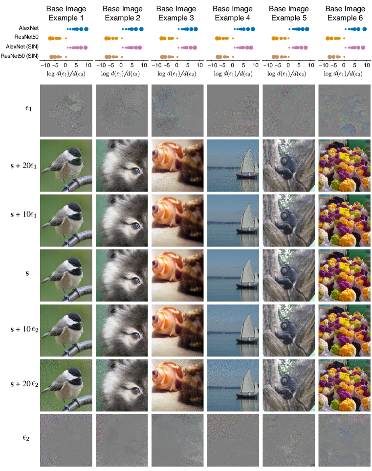
Figure 8: Principal distortions for standard ImageNet trained and Shape Image Net Trained (SIN) AlexNet and ResNet50 architectures for example base images.

The architectural difference observed between ImageNet-trained AlexNet and ResNet50 suggested that the texture of the image may be driving some of the differences in local geometry. Previous work demonstrated that standard DNNs exhibit strong “texture bias” (Geirhos et al., 2019) and proposed models that explicitly reduce the texture bias by training on Stylized ImageNet (SIN), a set of images that retains the content of each ImageNet image but overlays details matched to particular texture. Training on these images can reduce the model’s reliance on texture for classification. If this training set strongly affected the local geometry of the networks, we might expect that principal distortions generated for a mixture of architectures and training sets would be driven by this training set distinction. We find evidence that this is not the case. We generated principal distortions for 100 base images using a set of layers from two architectures (ResNet50 and AlexNet) and two different training datasets (ImageNet and Stylized ImageNet) (Fig. 4A). The principal distortions appeared qualitatively similar to those generated when we investigated only the standard networks (Fig. 4B, more examples in Fig. 8 of the supplement). Both AlexNet architectures, regardless of the training type, were more sensitive to the perturbations of higher variability parts of the image, while both ResNet50 models were more sensitive to the distortions that were mainly targeting constant areas of the image.

Networks trained to reduce adversarial vulnerability

Another well-known example of the use of training set modifications to achieve robustness in object recognition is that of adversarial training (AT). Adversarial examples are generated at each step of model training and these stimuli are used to update the model weights, with the “true” category label used for the update. Previous work has found that adversarially-trained networks are more aligned with those of biological systems (Madry, 2017; Feather et al., 2023; Gaziv et al., 2023). As adversarial examples are constrained to be very small perturbations, it seems plausible that the local geometry for AT models would differ from their standard counterparts. Indeed, we see that the principal distortions generated from the set of models that included standard and AT trained AlexNet and ResNet50 models reliably separate the model classes by training type, rather than architecture (Fig. 5A). Most layers of the adversarially trained models are more sensitive to relatively smooth changes of patches of color in the image, or to shading around edges, while most layers of the standard models are more sensitive to what appears as unstructured noise (Fig. 5B, additional examples in Fig. 9 of the supplement). This is in stark contrast to the style-trained networks of the previous section, for which principal distortions reliably separated the models by architecture. These examples provide a compelling demonstration that our method can be used to separate collections of similar models, and points to its utility in probing complex high-level representations.

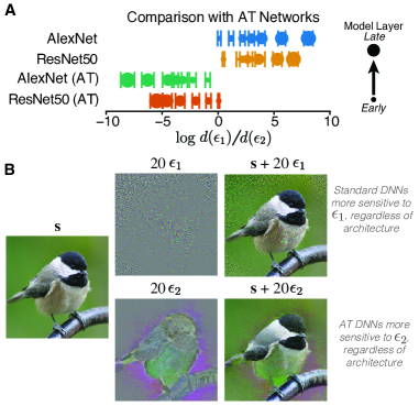
Figure 5: Comparison of AlexNet and ResNet50 variants trained to reduce adversarial vulnerability. A) Log sensitivity ratios of principal distortions for different layers of standard-trained and adversarially-trained (AT) models. Average log sensitivity is computed across 100 base images (error bars are standard deviation) and the choice of ${\bm{\epsilon}}_{1}$ is set such that $d({\bm{\epsilon}}_{1})\geq 0$ for the last tested layer of the standard AlexNet. B) Example base image and the generated principal distortions. Distortion ${\bm{\epsilon}}_{1}$ appears as less structured noise, and both AlexNet and ResNet50 standard networks are more sensitive to this perturbation, while the AT DNNs are more sensitive to ${\bm{\epsilon}}_{2}$ which focuses color changes around the content of the image, suggesting that the differences in local sensitivities of these networks depend more on differences in training procedure than architecture.

5 Discussion

We have introduced a metric on image representations that quantifies differences in local geometry, and used it to synthesize “principal distortions” that maximize the variance of the metric over a set of models. When applied to hand-engineered models of the early visual system and to deep neural networks, our approach produced novel distortions for distinguishing the corresponding models. In particular, with the DNN analysis, we revealed that there are qualitative differences in local geometries of ResNet50 and AlexNet architectures, that adversarial training dramatically changes the local geometry, but stylized ImageNet training does not. Although our qualitative examples in this targeted set of neural networks do not fully elucidate the recent observations that many different models are equally good at capturing brain representations, our method provides a direct approach to begin to tease apart the interplay between local geometry and global structure.

There are several natural methodological extensions. The metric is closely related to the Fisher-Rao metric between mean zero Gaussians and this relation suggests a natural extension to synthesizing more than two distortions (Appx. A), analogous to using additional principal components to capture more variance within a set of high-dimensional vectors. Additionally, while we focus on computing principal distortions that differentiate a finite set of models, there is a natural extension to computing the principal distortions that differentiate continuous families of models with a prior distribution over models.

There are several limitations in our formulation of principal distortions. First, our framework is based on local differential analyses of a model at a base image, so the sensitivity estimates we obtain via these analyses can only be guaranteed to hold in an infinitesimally small neighborhood of the base image. If a model is highly nonlinear in the vicinity of a base image, then the local linear approximation may not accurately reflect model sensitivities. Second, to compute the FIM of a deterministic model, we assume additive Gaussian response noise, which is not generally representative of neural responses in the brain. Poisson variability could be used to better capture neural responses. Another approach is to fit the model noise structure to measurements of a neural system; see (Ding et al., 2023) for work along these lines.

Principal distortions provide an efficient method for comparing computational models with human observers, for whom experimental time for acquiring responses to stimuli is generally severely limited. Although we only presented qualitative comparisons and examples related to human perception in this paper, the optimized distortions are a parsimonious choice of stimuli that can be readily incorporated into psychophysics experiments. For example, the distortions generated from the early visual models could be used for a perceptual discrimination experiment with human observers similar to those performed by Berardino et al. (2017), to compare the human log-ratio sensitivity for the optimized distortions to that predicted by the models.

The results with DNNs reveal some intriguing properties: some models have stronger sensitivity biases in the local geometry for perturbing higher variability regions of the space, while others have more sensitivity to perturbations in relatively blank regions (see Fig. 7 of the supplement for direct evidence of this). This also provides and interesting question for future distortion detection: in what contexts are humans more sensitive to perturbations of the “stuff” of the image compared to perturbations in empty parts of the image? And how do these observed differences relate to previous work investigating how human and neural networks rely on on spatial frequencies for classification (Subramanian et al., 2023)? Finally, beyond direct comparisons with human observers using psychophysics experiments, our method may be useful in the domain of neural network interpretability, where it may be useful to have direct comparisons of the local distortions that will maximally differentiate sets of models.

6 Reproducibility Statement

The code used to generate principal distortions and details of loading the models is uploaded as a .zip file for the submission, and will be made available via a public GitHub repository upon publication. We aim for the distortion generation to be easy for others to use to probe new models. The mathematical derivation of the algorithm is provided in Appx. B. We have included details in Appx. C with the parameters of the early visual models, and Appx. D details where checkpoints were obtained for the tested deep neural networks.

Appendix A Relation to the Fisher-Rao metric

The Fisher-Rao distance between two mean zero $K$-dimensional Gaussian distributions with positive definite covariance matrices ${\bm{A}}$ and ${\bm{B}}$ is defined as:

$$\delta^{2}({\bm{A}},{\bm{B}}):=\|\log({\bm{B}}^{-1/2}{\bm{A}}{\bm{B}}^{-1/2})\|_{F}^{2}=\sum_{i=1}^{K}(\log\lambda_{i})^{2},$$

where $\{\lambda_{i}\}$ denote the eigenvalues of the generalized eigenvalue problem ${\bm{A}}{\bm{v}}=\lambda{\bm{B}}{\bm{v}}$ (Pinele et al., 2020). We’d like a metric that’s invariant to arbitrary scalings ${\bm{A}}\mapsto c_{A}{\bm{A}}$ or ${\bm{B}}\mapsto c_{B}{\bm{B}}$ for $c_{A},c_{B}>0$, which suggests the following definition:

$$\gamma^{2}({\bm{A}},{\bm{B}})=\min_{c_{A},c_{B}>0}\delta^{2}(c_{A}{\bm{A}},c_{B}{\bm{B}})=\min_{c\in\mathbb{R}}\sum_{i=1}^{K}(c+\log\lambda_{i})^{2}=K\text{Var}(\{\log\lambda_{i}\}),$$ (5)

where the final equality uses the fact that the optimal $c$ is the mean of $\{-\log\lambda_{i}\}$.

Using the facts that

$$K\text{Var}(\{\log\lambda_{i}\}) =\frac{1}{2K}\sum_{i=1}^{K}\sum_{j=1}^{K}(\log\lambda_{i}-\log\lambda_{j})^{2},$$

and $(\log\lambda_{i}-\log\lambda_{j})^{2}\leq(\log\lambda_{1}-\log\lambda_{K})^{2}$ for all $i,j$, we have

$$\frac{1}{K}(\log\lambda_{1}-\log\lambda_{K})^{2}\leq\gamma^{2}({\bm{A}},{\bm{B}})\leq\frac{K-1}{2}(\log\lambda_{1}-\log\lambda_{K})^{2}.$$

When ${\bm{A}}={\bm{I}}_{A}$ and ${\bm{B}}={\bm{I}}_{B}$, then $d_{A}({\bm{\epsilon}})=\sqrt{{\bm{\epsilon}}^{\top}{\bm{A}}{\bm{\epsilon}}}$ and $d_{B}({\bm{\epsilon}})=\sqrt{{\bm{\epsilon}}^{\top}{\bm{B}}{\bm{\epsilon}}}$. If ${\bm{\epsilon}}_{1}$ and ${\bm{\epsilon}}_{K}$ denote the extremal generalized eigenvectors associated with $\lambda_{1}$ and $\lambda_{K}$, respectively, then

$$\log\lambda_{1}=2\log\frac{d_{A}({\bm{\epsilon}}_{1})}{d_{B}({\bm{\epsilon}}_{1})}, \log\lambda_{K}=2\log\frac{d_{A}({\bm{\epsilon}}_{K})}{d_{B}({\bm{\epsilon}}_{K})}.$$

Therefore,

$$\frac{2}{\sqrt{K}}\left|\log\frac{d_{A}({\bm{\epsilon}}_{1})}{d_{B}({\bm{\epsilon}}_{1})}-\log\frac{d_{A}({\bm{\epsilon}}_{K})}{d_{B}({\bm{\epsilon}}_{K})}\right|\leq\gamma({\bm{A}},{\bm{B}})\leq\sqrt{2(K-1)}\left|\log\frac{d_{A}({\bm{\epsilon}}_{1})}{d_{B}({\bm{\epsilon}}_{1})}-\log\frac{d_{A}({\bm{\epsilon}}_{K})}{d_{B}({\bm{\epsilon}}_{K})}\right|,$$

and so

$$\frac{2}{\sqrt{K}}m_{{\bm{\epsilon}}_{1},{\bm{\epsilon}}_{K}}({\bm{I}}_{A},{\bm{I}}_{B})\leq\gamma({\bm{A}},{\bm{B}})\leq\sqrt{2(K-1)}m_{{\bm{\epsilon}}_{1},{\bm{\epsilon}}_{K}}({\bm{I}}_{A},{\bm{I}}_{B}).$$

Extension to more than two distortions

Equation 5 suggests a natural extension for defining a metric between positive definite matrices using $M>2$ distortions. Specifically, it suggests choosing the distortions to maximize the variance across the log ratios of the sensitivities. To this end, we can define the squared distance between the local geometries to be the variance (across distortions) of the log ratio of the the sensitivities:

$$m_{{\bm{\epsilon}}_{1},\dots,{\bm{\epsilon}}_{M}}^{2}({\bm{A}},{\bm{B}})=M\text{Var}\left(\left\{\log\frac{d_{A}({\bm{\epsilon}}_{m})}{d_{B}({\bm{\epsilon}}_{m})}\right\}\right).$$

A set of $M$ principal distortions can then be chosen to maximize the variance across models under this metric.

Appendix B Computing the top two optimal distortions

Suppose we have $N$ models with sensitivities $\{d_{n}({\bm{\epsilon}})\}$. The optimal distortions $\{{\bm{\epsilon}}_{1},{\bm{\epsilon}}_{2}\}$ are solutions to the optimization problem

$$\operatorname*{arg\,max}_{{\bm{\epsilon}}_{1},{\bm{\epsilon}}_{2}}L({\bm{\epsilon}}_{1},{\bm{\epsilon}}_{2}), L({\bm{\epsilon}}_{1},{\bm{\epsilon}}_{2}):=\sum_{n=1}^{N}\left\{\log\frac{d_{n}({\bm{\epsilon}}_{1})}{d_{n}({\bm{\epsilon}}_{2})}-\frac{1}{N}\sum_{m=1}^{N}\log\frac{d_{m}({\bm{\epsilon}}_{1})}{d_{m}({\bm{\epsilon}}_{2})}\right\}^{2}.$$

Differentiating $L$ with respect to ${\bm{\epsilon}}_{1}$ yields

$$\nabla_{{\bm{\epsilon}}_{1}}L({\bm{\epsilon}}_{1},{\bm{\epsilon}}_{2}) =2\sum_{n=1}^{N}\left\{\log\frac{d_{n}({\bm{\epsilon}}_{1})}{d_{n}({\bm{\epsilon}}_{2})}-\frac{1}{N}\sum_{m=1}^{N}\log\frac{d_{m}({\bm{\epsilon}}_{1})}{d_{m}({\bm{\epsilon}}_{2})}\right\}\left\{\frac{{\bm{I}}_{n}({\mathbf{s}}){\bm{\epsilon}}_{1}}{d_{n}^{2}({\bm{\epsilon}}_{1})}-\frac{1}{N}\sum_{m=1}^{N}\frac{{\bm{I}}_{m}({\mathbf{s}}){\bm{\epsilon}}_{1}}{d_{m}^{2}({\bm{\epsilon}}_{1})}\right\}$$

$$=\sum_{n=1}^{N}\left\{\log\frac{d_{n}^{2}({\bm{\epsilon}}_{1})}{d_{n}^{2}({\bm{\epsilon}}_{2})}-\frac{1}{N}\sum_{m=1}^{N}\log\frac{d_{m}^{2}({\bm{\epsilon}}_{1})}{d_{m}^{2}({\bm{\epsilon}}_{2})}\right\}\left\{\frac{{\bm{I}}_{n}({\mathbf{s}}){\bm{\epsilon}}_{1}}{d_{n}^{2}({\bm{\epsilon}}_{1})}-\frac{1}{N}\sum_{m=1}^{N}\frac{{\bm{I}}_{m}({\mathbf{s}}){\bm{\epsilon}}_{1}}{d_{m}^{2}({\bm{\epsilon}}_{1})}\right\},$$

where we have used the fact that

$$\nabla_{{\bm{\epsilon}}}\log d({\bm{\epsilon}}) =\frac{1}{2}\nabla_{{\bm{\epsilon}}}\log({\bm{\epsilon}}^{\top}{\bm{I}}{\bm{\epsilon}})=\frac{{\bm{I}}{\bm{\epsilon}}}{{\bm{\epsilon}}^{\top}{\bm{I}}{\bm{\epsilon}}}=\frac{{\bm{I}}{\bm{\epsilon}}}{d^{2}({\bm{\epsilon}})}.$$

Similarly, differentiating $L$ with respect to ${\bm{\epsilon}}_{2}$ yields:

$$\nabla_{{\bm{\epsilon}}_{2}}L({\bm{\epsilon}}_{1},{\bm{\epsilon}}_{2}) =-\sum_{n=1}^{N}\left\{\log\frac{d_{n}^{2}({\bm{\epsilon}}_{1})}{d_{n}^{2}({\bm{\epsilon}}_{2})}-\frac{1}{N}\sum_{m=1}^{N}\log\frac{d_{m}^{2}({\bm{\epsilon}}_{1})}{d_{m}^{2}({\bm{\epsilon}}_{2})}\right\}\left\{\frac{{\bm{I}}_{n}({\mathbf{s}}){\bm{\epsilon}}_{2}}{d_{n}^{2}({\bm{\epsilon}}_{2})}-\frac{1}{N}\sum_{m=1}^{N}\frac{{\bm{I}}_{m}({\mathbf{s}}){\bm{\epsilon}}_{2}}{d_{m}^{2}({\bm{\epsilon}}_{2})}\right\}.$$

Combining, we have the following gradient-based optimization algorithm.

1:  Input: Positive definite $D\times D$ matrices ${\bm{I}}_{1},\dots,{\bm{I}}_{N}$, learning rate $\eta>0$, target distortion size $\alpha>0$

2:  Initialize: distortions ${\bm{\epsilon}}_{1},{\bm{\epsilon}}_{2}\in\mathbb{R}^{D}$

3:  while not converged do

4:     for $n=1,\dots,N$ do

5:        ${\bm{v}}_{1}(n)\leftarrow{\bm{I}}_{n}{\bm{\epsilon}}_{1}$

6:        ${\bm{v}}_{2}(n)\leftarrow{\bm{I}}_{n}{\bm{\epsilon}}_{2}$

7:        $d_{1}^{2}(n)\leftarrow\langle{\bm{\epsilon}}_{1},{\bm{v}}_{1}(n)\rangle$

8:        $d_{2}^{2}(n)\leftarrow\langle{\bm{\epsilon}}_{2},{\bm{v}}_{2}(n)\rangle$

9:        ${\bm{u}}_{1}(n)={\bm{v}}_{1}(n)/d_{1}^{2}(n)$

10:        ${\bm{u}}_{2}(n)={\bm{v}}_{2}(n)/d_{2}^{2}(n)$

11:        $r(n)\leftarrow\log d_{1}^{2}(n)-\log d_{2}^{2}(n)$

12:     end for

13:     $\bar{\bm{u}}_{1}\leftarrow\text{mean}({\bm{u}}_{1}(n))$

14:     $\bar{\bm{u}}_{2}\leftarrow\text{mean}({\bm{u}}_{2}(n))$

15:     $\bar{r}\leftarrow\text{mean}(r(n))$

16:     $\Delta{\bm{\epsilon}}_{1}\leftarrow\sum_{n=1}^{N}\left[r(n)-\bar{r}\right]\left[{\bm{u}}_{1}(n)-\bar{\bm{u}}_{1}\right]$

17:     $\Delta{\bm{\epsilon}}_{2}\leftarrow-\sum_{n=1}^{N}\left[r(n)-\bar{r}\right]\left[{\bm{u}}_{2}(n)-\bar{\bm{u}}_{2}\right]$

18:     ${\bm{\epsilon}}_{1}\leftarrow{\bm{\epsilon}}_{1}+\eta\Delta{\bm{\epsilon}}_{1}$

19:     ${\bm{\epsilon}}_{2}\leftarrow{\bm{\epsilon}}_{2}+\eta\Delta{\bm{\epsilon}}_{2}$

20:     ${\bm{\epsilon}}_{1}\leftarrow\alpha{\bm{\epsilon}}_{1}/\|{\bm{\epsilon}}_{1}\|$

21:     ${\bm{\epsilon}}_{2}\leftarrow\alpha{\bm{\epsilon}}_{2}/\|{\bm{\epsilon}}_{2}\|$

22:  end while

Algorithm 1 Computing the principal distortions via projected gradient descent

Appendix C Methods: Early Visual Model Experiments

PyTorch implementations of the early visual models were obtained from (https://github.com/plenoptic-org/plenoptic, Duong et al., 2023a). The early visual models were adopted from Berardino et al. (2017), with parameters chosen to maximize the correlation between predicted perceptual distance and human ratings of perceived distortion, for a wide range of images and distortions provided in the TID-2008 database (Ponomarenko et al., 2009). Parameters are reported in Table 1. Note that although the models are nested in their construction and parameterization, the model parameters differ across tested models since they are optimized for each model independently.

LN Model
center-surround, center std	0.5339
center-surround, surround std	6.148
center-surround, amplitude ratio	1.25
LG Model
luminance, scalar	14.95
luminance, std	4.235
center-surround, center std	1.962
center-surround, surround std	4.235
center-surround, amplitude ratio	1.25
LGG Model
luminance, scalar	2.94
contrast, scalar	34.03
center-surround, center std	0.7363
center-surround, surround std	48.37
center-surround, amplitude ratio	1.25
luminance, std	170.99
contrast, std	2.658
LGN Model	(Two channels)
luminance, scalar	[3.2637, 14.3961]
contrast, scalar	[7.3405, 16.7423]
center-surround, center std	[1.237, 0.3233]
center-surround, surround std	[30.12, 2.184]
center-surround, amplitude ratio	1.25
luminance, std	[76.4, 2.184]
contrast, std	[7.49, 2.43]

Table 1: Parameters for early visual models, obtained from (Berardino et al., 2017).

Appendix D Methods: Deep Neural Network Experiments

The analyzed DNNs were obtained from the model loading code and checkpoints available at https://github.com/jenellefeather/model_metamers_pytorch which were used in Feather et al. (2023), and allowed for easy loading and selection of the intermediate layer stages for many models that had previously been proposed as models of human visual perception. The checkpoints for the standard ResNet50 and AlexNet models were obtained from the public pytorch checkpoints ((Ansel et al., 2024)). The Stylized Image Net AlexNet (alexnet_trained_on_SIN) and ResNet50 (resnet50_trained_on_SIN) were obtained from https://github.com/rgeirhos/texture-vs-shape associated with Geirhos et al. (2019). The checkpoint for the ResNet50 $\ell_{2}(\epsilon_{\text{train}}=3.0)$ adversarially trained model was obtained from Engstrom et al. (2019), and the checkpoint for the Alexnet $\ell_{2}(\epsilon_{\text{train}}=3.0)$ adversarially trained model was obtained from Feather et al. (2023). For all experiments, we only included intermediate layers before the final classification stage in the principal distortion analysis, and the subset of layers followed those chosen in Feather et al. (2023). Specifically, for the AlexNet models we included layers relu0, relu1, relu2, relu3, relu4, fc0_relu, and fc1_relu in each set of anlayses. For the ResNet50 models we included conv1_relu1, layer1, layer2, layer3, layer4, and avgpool in each set of analyses.

D.1 Principal distortion optimization

For the deep neural network experiments, we use a subset of 100 ImageNet images where each image was chosen from a unique class (randomly chosen from the set of images at https://github.com/EliSchwartz/imagenet-sample-images). For each image and each comparison, we ran the gradient descent procedure for principal distortion optimization for 2500 iterations, using an exponentially decaying learning rate that started at 10.0 and decayed to 0.001 by the final step.

We used a target distortion size of $\alpha=0.1$ and at each step of the optimization, we also scaled ${\bm{\epsilon}}$ so that the image ${\mathbf{s}}+1000{\bm{\epsilon}}$ would not be clipped when the RGB value was represented between 0–1; that is, we scaled ${\bm{\epsilon}}$ so that $0\leq s[i]+1000\epsilon[i]\leq 1$ for each value $i$ in the image. This constraint could potentially bias the perturbations to be more spread out across the image (because all of the amplitude for the perturbation cannot be focused at a small set of pixels). However, removing this constraint did not lead to quantitatively different results (Supplementary Fig. 10), but the inclusion allows for more viable comparisons with human perception (as the perturbation can be scaled while maintaining valid values in the image gamut).

D.2 Supplemental Figures

Figure 9: Principal distortions for standard ImageNet trained and adversarially trained AlexNet and ResNet50 architectures for example base images.

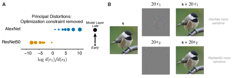
Figure 10: Example principal distortions for ResNet50 vs. AlexNet comparison where the pixelwise min/max value for the perturbation has not been constrained to avoid clipping once the perturbation is scaled. Similar to the results in the main text, we see that the principal distortion that AlexNet is more sensitive to is focused on the part of the image with high-contrast texture features, while ResNet50 is more sensitive to the perturbation targeting relatively blank parts of the image.

References

- Amari (2016) Shun-ichi Amari. Information Geometry and its Applications, volume 194. Springer, 2016.
- Ansel et al. (2024) Jason Ansel, Edward Yang, Horace He, Natalia Gimelshein, Animesh Jain, Michael Voznesensky, Bin Bao, Peter Bell, David Berard, Evgeni Burovski, Geeta Chauhan, Anjali Chourdia, Will Constable, Alban Desmaison, Zachary DeVito, Elias Ellison, Will Feng, Jiong Gong, Michael Gschwind, Brian Hirsh, Sherlock Huang, Kshiteej Kalambarkar, Laurent Kirsch, Michael Lazos, Mario Lezcano, Yanbo Liang, Jason Liang, Yinghai Lu, CK Luk, Bert Maher, Yunjie Pan, Christian Puhrsch, Matthias Reso, Mark Saroufim, Marcos Yukio Siraichi, Helen Suk, Michael Suo, Phil Tillet, Eikan Wang, Xiaodong Wang, William Wen, Shunting Zhang, Xu Zhao, Keren Zhou, Richard Zou, Ajit Mathews, Gregory Chanan, Peng Wu, and Soumith Chintala. PyTorch 2: Faster Machine Learning Through Dynamic Python Bytecode Transformation and Graph Compilation. In 29th ACM International Conference on Architectural Support for Programming Languages and Operating Systems, Volume 2 (ASPLOS ’24). ACM, April 2024. doi: 10.1145/3620665.3640366. URL https://pytorch.org/assets/pytorch2-2.pdf.
- Averbeck & Lee (2006) Bruno B Averbeck and Daeyeol Lee. Effects of noise correlations on information encoding and decoding. Journal of Neurophysiology, 95(6):3633–3644, 2006.
- Berardino et al. (2017) Alexander Berardino, Johannes Ballé, Valero Laparra, and Eero P Simoncelli. Eigen-distortions of hierarchical representations. Advances in Neural Information Processing Systems, 30:3531–3540, 2017.
- Brunel & Nadal (1998) Nicolas Brunel and Jean-Pierre Nadal. Mutual information, Fisher information, and population coding. Neural Computation, 10(7):1731–1757, 1998.
- Burg et al. (2024) Max F Burg, Thomas Zenkel, Michaela Vystrčilová, Jonathan Oesterle, Larissa Höfling, Konstantin Friedrich Willeke, Jan Lause, Sarah Müller, Paul G. Fahey, Zhiwei Ding, Kelli Restivo, Shashwat Sridhar, Tim Gollisch, Philipp Berens, Andreas S. Tolias, Thomas Euler, Matthias Bethge, and Alexander S Ecker. Most discriminative stimuli for functional cell type clustering. In The Twelfth International Conference on Learning Representations, 2024. URL https://openreview.net/forum?id=9W6KaAcYlr.
- Chung & Abbott (2021) SueYeon Chung and Larry F Abbott. Neural population geometry: An approach for understanding biological and artificial neural networks. Current opinion in neurobiology, 70:137–144, 2021.
- Conwell et al. (2022) Colin Conwell, Jacob S Prince, Kendrick N Kay, George A Alvarez, and Talia Konkle. What can 1.8 billion regressions tell us about the pressures shaping high-level visual representation in brains and machines? BioRxiv, pp. 2022–03, 2022.
- Cramér (1946) Harald Cramér. Mathematical Methods of Statistics, volume 26. Princeton University Press, 1946.
- Ding et al. (2023) Xuehao Ding, Dongsoo Lee, Joshua B Melander, George Sivulka, Surya Ganguli, and Stephen A Baccus. Information geometry of the retinal representation manifold. Advances in Neural Information Processing Systems, 36:44310–44322, 2023.
- Duong et al. (2023a) Lyndon Duong, Kathryn Bonnen, William Broderick, Pierre-Étienne Fiquet, Nikhil Parthasarathy, Thomas Yerxa, Xinyuan Zhao, and Eero Simoncelli. Plenoptic: A platform for synthesizing model-optimized visual stimuli. Journal of Vision, 23(9):5822–5822, 2023a.
- Duong et al. (2023b) Lyndon Duong, Jingyang Zhou, Josue Nassar, Jules Berman, Jeroen Olieslagers, and Alex H Williams. Representational dissimilarity metric spaces for stochastic neural networks. In The Eleventh International Conference on Learning Representations, 2023b.
- Engstrom et al. (2019) Logan Engstrom, Andrew Ilyas, Hadi Salman, Shibani Santurkar, and Dimitris Tsipras. Robustness (python library), 2019. URL https://github.com/MadryLab/robustness.
- Feather et al. (2023) Jenelle Feather, Guillaume Leclerc, Aleksander Madry, and Josh H McDermott. Model metamers reveal divergent invariances between biological and artificial neural networks. Nature Neuroscience, 26(11):2017–2034, 2023.
- Fisher (1925) Ronald Aylmer Fisher. Theory of statistical estimation. Mathematical Proceedings of the Cambridge Philosophical Society, 22(5):700–725, 1925.
- Ganguli & Simoncelli (2014) Deep Ganguli and Eero P Simoncelli. Efficient sensory encoding and bayesian inference with heterogeneous neural populations. Neural Computation, 26(10):2103–2134, 2014.
- Gaziv et al. (2023) Guy Gaziv, Michael J Lee, and James J DiCarlo. Robustified anns reveal wormholes between human category percepts. arXiv preprint arXiv:2308.06887, 2023.
- Geirhos et al. (2019) Robert Geirhos, Patricia Rubisch, Claudio Michaelis, Matthias Bethge, Felix A. Wichmann, and Wieland Brendel. ImageNet-trained CNNs are biased towards texture; increasing shape bias improves accuracy and robustness. In International Conference on Learning Representations, 2019.
- Golan et al. (2020) Tal Golan, Prashant C Raju, and Nikolaus Kriegeskorte. Controversial stimuli: Pitting neural networks against each other as models of human cognition. Proceedings of the National Academy of Sciences, 117(47):29330–29337, 2020.
- Goodfellow et al. (2014) Ian J Goodfellow, Jonathon Shlens, and Christian Szegedy. Explaining and harnessing adversarial examples. International Conference on Learning Representations, 2014.
- Green & Swets (1966) D.M. Green and J.A. Swets. Signal Detection Theory and Psychophysics. Wiley, New York, 1966.
- He et al. (2016) Kaiming He, Xiangyu Zhang, Shaoqing Ren, and Jian Sun. Deep residual learning for image recognition. In Proceedings of the IEEE conference on computer vision and pattern recognition, pp. 770–778, 2016.
- Klabunde et al. (2023) Max Klabunde, Tobias Schumacher, Markus Strohmaier, and Florian Lemmerich. Similarity of neural network models: A survey of functional and representational measures. arXiv preprint arXiv:2305.06329, 2023.
- Kornblith et al. (2019) Simon Kornblith, Mohammad Norouzi, Honglak Lee, and Geoffrey Hinton. Similarity of neural network representations revisited. In International conference on machine learning, pp. 3519–3529. PMLR, 2019.
- Kriegeskorte et al. (2008) Nikolaus Kriegeskorte, Marieke Mur, and Peter A Bandettini. Representational similarity analysis-connecting the branches of systems neuroscience. Frontiers in Systems Neuroscience, 2:249, 2008.
- Krizhevsky et al. (2012) Alex Krizhevsky, Ilya Sutskever, and Geoffrey E Hinton. Imagenet classification with deep convolutional neural networks. Advances in neural information processing systems, 25, 2012.
- Lindsay (2021) Grace W Lindsay. Convolutional neural networks as a model of the visual system: Past, present, and future. Journal of cognitive neuroscience, 33(10):2017–2031, 2021.
- Lipshutz et al. (2024) David Lipshutz, Jenelle Feather, Sarah E Harvey, Alex H Williams, and Eero P Simoncelli. Comparing the local information geometry of image representations. In UniReps: 2nd Edition of the Workshop on Unifying Representations in Neural Models, 2024.
- Madry (2017) Aleksander Madry. Towards deep learning models resistant to adversarial attacks. arXiv preprint arXiv:1706.06083, 2017.
- Paradiso (1988) MA Paradiso. A theory for the use of visual orientation information which exploits the columnar structure of striate cortex. Biological Cybernetics, 58(1):35–49, 1988.
- Pinele et al. (2020) Julianna Pinele, João E Strapasson, and Sueli IR Costa. The Fisher-Rao distance between multivariate normal distributions: Special cases, bounds and applications. Entropy, 22(4):404, 2020.
- Ponomarenko et al. (2009) Nikolay Ponomarenko, Vladimir Lukin, Alexander Zelensky, Karen Egiazarian, Marco Carli, and Federica Battisti. Tid2008-a database for evaluation of full-reference visual quality assessment metrics. Advances of modern radioelectronics, 10(4):30–45, 2009.
- Rao (1945) C R Rao. Information and accuracy attainable in the estimation of statistical parameters. Bulletin of the Calcutta Mathematical Society, 37(3):81–91, 1945.
- Schrimpf et al. (2018) Martin Schrimpf, Jonas Kubilius, Ha Hong, Najib J Majaj, Rishi Rajalingham, Elias B Issa, Kohitij Kar, Pouya Bashivan, Jonathan Prescott-Roy, Franziska Geiger, et al. Brain-score: Which artificial neural network for object recognition is most brain-like? BioRxiv, pp. 407007, 2018.
- Seriès et al. (2009) Peggy Seriès, Alan A Stocker, and Eero P Simoncelli. Is the homunculus “aware” of sensory adaptation? Neural Computation, 21(12):3271–3304, 2009.
- Seung & Sompolinsky (1993) HS Seung and H Sompolinsky. Simple models for reading neuronal population codes. Proceedings of the National Academy of Sciences of the United States of America, 90:10749–10753, 1993.
- Subramanian et al. (2023) Ajay Subramanian, Elena Sizikova, Najib J. Majaj, and Denis G. Pelli. Spatial-frequency channels, shape bias, and adversarial robustness. In Thirty-seventh Conference on Neural Information Processing Systems, 2023. URL https://openreview.net/forum?id=KvPwXVcslY.
- Szegedy et al. (2013) Christian Szegedy, Wojciech Zaremba, Ilya Sutskever, Joan Bruna, Dumitru Erhan, Ian Goodfellow, and Rob Fergus. Intriguing properties of neural networks. arXiv preprint arXiv:1312.6199, 2013.
- Tuckute et al. (2023) Greta Tuckute, Jenelle Feather, Dana Boebinger, and Josh H McDermott. Many but not all deep neural network audio models capture brain responses and exhibit correspondence between model stages and brain regions. Plos Biology, 21(12):e3002366, 2023.
- Wang & Simoncelli (2008) Zhou Wang and Eero P Simoncelli. Maximum differentiation (MAD) competition: A methodology for comparing computational models of perceptual quantities. Journal of Vision, 8(12):8–8, 2008.
- Wei & Stocker (2016) Xue-Xin Wei and Alan A Stocker. Mutual information, Fisher information, and efficient coding. Neural Computation, 28(2):305–326, 2016.
- Williams et al. (2021) Alex H Williams, Erin Kunz, Simon Kornblith, and Scott Linderman. Generalized shape metrics on neural representations. Advances in Neural Information Processing Systems, 34:4738–4750, 2021.
- Yamins & DiCarlo (2016) Daniel LK Yamins and James J DiCarlo. Using goal-driven deep learning models to understand sensory cortex. Nature Neuroscience, 19(3):356–365, 2016.
- Zhou et al. (2023) Jingyang Zhou, Chanwoo Chun, Ajay Subramanian, and Eero P Simoncelli. Comparing neural models using their perceptual discriminability predictions. In Proceedings of UniReps: the First Workshop on Unifying Representations in Neural Models, pp. 170–181. PMLR, 2023.