Conditional Uncertainty Quantification for Tensorized Topological Neural Networks
Abstract
Graph Neural Networks (GNNs) have become the de facto standard for analyzing graph-structured data, leveraging message-passing techniques to capture both structural and node feature information. However, recent studies have raised concerns about the statistical reliability of uncertainty estimates produced by GNNs. This paper addresses this crucial challenge by introducing a novel technique for quantifying uncertainty in non-exchangeable graph-structured data, while simultaneously reducing the size of label prediction sets in graph classification tasks. We propose Conformalized Tensor-based Topological Neural Networks (CF-T²NN), a new approach for rigorous prediction inference over graphs. CF-T²NN employs tensor decomposition and topological knowledge learning to navigate and interpret the inherent uncertainty in decision-making processes. This method enables a more nuanced understanding and handling of prediction uncertainties, enhancing the reliability and interpretability of neural network outcomes. Our empirical validation, conducted across 10 real-world datasets, demonstrates the superiority of CF-T²NN over a wide array of state-of-the-art methods on various graph benchmarks. This work not only enhances the GNN framework with robust uncertainty quantification capabilities but also sets a new standard for reliability and precision in graph-structured data analysis.
Keywords Uncertainty quantification Conditional Prediction Set Tensor Decomposition Graph Classification
1 Introduction
Graph neural networks (GNNs) have emerged as a powerful machinery for various graph learning tasks, such as link prediction, node, and graph classification [1, 2]. Their ability to effectively model relational data has transformed our approach to understanding complex systems, including social networks [3], biochemical structures [4], traffic networks [5]. As GNNs increasingly play a role in critical decision-making in social and medical applications, the accuracy of their predictions and their reliability have become paramount. In particular, the uncertainty quantification of label prediction is of great interest in practice. For example, a predicted probability of and for labels A and B will both lead to predicted label B, but the confidence level will be quite different for the two cases. Thus, an increasing number of researchers are focusing on the uncertainty of predictions made by GNNs [6, 7, 8, 9]. A recent survey [10] summarizes several uncertainty quantification approaches, including Bayesian-based methods. Nonetheless, many techniques frequently fall short in providing both theoretical and empirical assurances about their accuracy, specifically the likelihood that the predicted set or interval encompasses the actual outcome [11]. This deficiency in precision impedes their trustworthy application in contexts where mistakes may have significant repercussions.
Conformal prediction [12] (CP) is a framework for producing statistically guaranteed prediction with uncertainty quantification. The general idea is to assess the conformity level of the potential value of outcome with respect to the observed data. So conformity, or in other words, “exchangeability”, is a crucial assumption for this method. This assumption is easily violated if there are covariate shifts or covariate constraints in the graph features which is commonly observed in large data sets. Here covariate shifts mean the distribution of the covariates is different, and covariate constraints mean the target of prediction is in a single or sub-type of graph features. Most works in GNN uncertainty quantification do not deal with those issues [13, 14]. Existing works focusing on non-exchangeable cases are often developed by adjusting the conformal prediction interval according to the estimated covariate shift [15, 16]. However, they are not directly applicable to GNNs where the shifts of graph covariates are hard to estimate. They are not applicable to the case where the target is to quantify the uncertainty of a single or certain type of graph.
To address this challenge, we develop a novel algorithm that produces a statistically coverage-guaranteed conditional prediction set under possible graph covariate shifts. This set not only offers guaranteed coverage under a relaxed condition of exchangeability, accommodating potential domain shifts in graph data but also innovates by requiring the existence of a local calibration set that contains “similar graph data" as the target. Termed the "local exchangeable" condition, this approach significantly enhances the adaptability of prediction models.
The primary obstacle in employing this conditional prediction set lies in the construction of the local calibration set, a task complicated by the high-dimensional and multi-dimensional nature of graph data. To navigate this complexity, we have developed a methodology that leverages Tensorized Topological Neural Networks, crafting our similarity measures on the basis of tensorized graph structure and its low-rank tensor decompositions. This approach effectively captures the essence of multi-dimensionality while simultaneously reducing dimensionality, thus facilitating a more nuanced and accurate modeling of graph data.
Through rigorous empirical validation across ten real-world datasets, our proposed methodologies have demonstrated superior performance against a comprehensive range of leading-edge methods in various graph analysis benchmarks. This accomplishment not only strengthens the GNN framework with robust uncertainty quantification tools but also establishes a new benchmark for reliability and precision in the analysis of graph-structured data.
2 Related Work
Uncertainty Quantification.
Conformal prediction is an attractive framework for uncertainty quantification of GNN lable prediction. [13] and [14] provide prediction set with guaranteed coverage and controled sizes. However, [14] utilizes the propagation of node labels in the calibration set, whereas [13] employs the inefficiency of the calibration set itself as the criterion for optimization. Several procedures of conformal prediction are introduced in [17], including split conformal we adopted in this article, which is both theoretically and computationally easy. [18] provides a detailed discussion of its properties and introduces a new concept of conditional prediction inference that challenges the coverage guarantee for conformal prediction. Also shown in [19], conditional inference is impossible without additional assumptions. Thus we develop an algorithm to handle this issue by adopting the so-called “iFusion learning” idea [20, 21]: instead of using the randomly selected calibration set to quantify uncertainty, we use a subset that contains only “similar” items to make inference for our target.
Tensor Learning.
Tensors, representing multidimensional data, have become prominent across various scientific disciplines, including neuroimaging [22], economics [23, 24], international trade [25], recommendation systems [26], multivariate spatial-temporal data analysis [27], and biomedical applications [28, 29]. Key areas of tensor research encompass tensor decomposition [30, 29], tensor regression [22, 31, 32, 33], and unsupervised learning techniques such as tensor clustering [34, 35, 36].
Empirical studies have demonstrated the effectiveness of tensor-based classification methods across these fields, leading to the development of techniques including support tensor machines [37, 38], tensor discriminant analysis [39], tensor logistic regression [40], and tensor neural networks [41, 42]. Neural networks designed to process tensor inputs enable efficient analysis of high-dimensional data. However, most existing work employs tensors primarily for computation rather than statistical analysis. Notable advancements include the analysis of deep neural networks’ expressive power using tensor methods [43], which established an equivalence between neural networks and hierarchical tensor factorizations. The Tensor Contraction Layer (TCL) [44] introduced tensor contractions as trainable neural network layers, while the Tensor Regression Layer (TRL) [45] further regularized networks through regression weights. The Graph Tensor Network (GTN) [46] proposed a Tensor Network-based framework for describing neural networks using tensor mathematics and graphs for large, multi-dimensional data.
Despite these advancements, current neural networks with tensor inputs lack comprehensive theoretical and empirical exploration. The Tensor-view Topological Graph Neural Network (TTG-NN) [42] represents a step forward, introducing a novel class of topological deep learning built upon persistent homology, graph convolution, and tensor operations.
Persistent Homology.
Persistent homology (PH) [47, 48] is a suite of tools within TDA that has shown great promise in a broad range of domains including bioinformatics, material sciences, and social networks [49, 50]. One of the key benefits of PH is that it can capture subtle patterns in the data shape dynamics at multiple resolution scales. PH has been successfully integrated as a fully trainable topological layer into various machine learning and deep learning models [51], addressing such tasks as image classification [52], 2D/3D shape classification [53], molecules and biomolecular complexes representation learning [54], graph classification [55], and spatio-temporal prediction [56]. For example, [57] builds a neural network based on the DeepSet architecture [58] which can achieve end-to-end learning for topological features. [54] introduces multi-component persistent homology, multi-level persistent homology and electrostatic persistence for chemical and biological characterization, analysis, and modeling by using convolutional neural networks. [59] proposes a trainable topological layer that incorporates global topological information of a graph using persistent homology. [60] proposes a time-aware topological deep learning model that captures interactions and encodes encodes time-conditioned topological information. However, to the best of our knowledge, both TDA and PH have yet to be employed for uncertainty quantification.
3 Preliminaries
Problem Settings.
Let be an attributed graph, where is a set of nodes (), is a set of edges, and is a feature matrix of nodes (here is the dimension of the node features). Let be a symmetric adjacency matrix whose entries are if nodes and are connected and 0 otherwise (here is an edge weight and for unweighted graphs). Furthermore, represents the degree matrix of , that is . In the graph classification setting, we have a set of graphs , where each graph is associated with a label . We denote a sample consisting of a graph and its label as . The goal of the graph classification task is to take the graph as the input and predict its corresponding label. Given a graph , the trained model has a predicted label , which is the of the probability distribution over all possible labels, say . To apply the uncertainty quantification algorithm, our goal is to obtain a prediction set with a certain level of confidence for label . We split our dataset into four disjoint subset, , , , , of fixed size with pre-defined ratios. They correspond to training, validation, calibration, and test sets. The calibration set is withheld to apply conformal prediction later for uncertainty quantification.
Persistent Homology.
PH is a subfield in computational topology whose main goal is to detect, track and encode the evolution of shape patterns in the observed object along various user-selected geometric dimensions [47, 48, 61]. These shape patterns represent topological properties such as connected components, loops, and, in general, -dimensional "holes", that is, the characteristics of the graph that remain preserved at different resolutions under continuous transformations. By employing such a multi-resolution approach, PH addresses the intrinsic limitations of classical homology and allows for retrieving the latent shape properties of which may play an essential role in a given learning task. The key approach here is to select some suitable scale parameters and then to study changes in the shape of that occur as evolves with respect to . That is, we no longer study as a single object but as a filtration , induced by monotonic changes of . To ensure that the process of pattern selection and counting is objective and efficient, we build an abstract simplicial complex on each , which results in filtration of complexes . For example, for an edge-weighted graph , with the edge-weight function , we can set for each , , yielding the induced sublevel edge-weighted filtration. Similarly, we can consider a function on a node set , for example, node degree, which results in a sequence of induced subgraphs of with a maximal degree of for each and the associated degree sublevel set filtration. We can then record scales (birth) and (death) at which each topological feature first and last appear in the sublevel filtration . In this paper, to encode the above topological information presented in a PD into the embedding function, we use its vectorized representation, i.e., persistence image (PI) [62]. The PI is a finite-dimensional vector representation obtained through a weighted kernel density function and can be computed in the following two steps (see more details in Definition 1). First, we map the PD to an integrable function , which is referred to as a persistence surface. The persistence surface is constructed by summing weighted Gaussian kernels centered at each point in . In the second step, we integrate the persistence surface over each grid box to obtain the value of the .
Definition 1 (Persistence Image).
Let be a non-negative weight function for the persistence plane . The value of each pixel is defined as where is the transformation of the PD Dg (i.e., for each , ), , and and are the standard deviations of a differentiable probability distribution in the and directions respectively.
Conformal Prediction and Its Limitations.
Conformal prediction [17] typically imposes the “exchangeable” condition on , , and , that is
| (1) |
where is the joint distribution of and its label .
The goal of conformal prediction is to construct a prediction set of a predicted label for any graph , such that the unconditional coverage
| (2) |
for any user-chosen error rate , and the probability measure is defined for the joint data .
The “exchangeable” condition (1) is restrictive and can be violated in many applications. For example, we collect data and train the algorithm on a large population, but are only interested in applying the algorithm to a specific sub-population and and are non-exchangeable with and . In this paper, we relax this assumption extensively to allow for possible domain shifts/constrain in graph data sets.
4 Method
Tensor Transformation Layer.
The Tensor Transformation Layer (TTL) preserves the tensor structures of feature of dimension and hidden throughput. Let be any positive integer and collects the width of all layers.
A deep ReLU Tensor Neural Network is a function mapping taking the form of
| (3) |
where is an element-wise activation function. Affine transformation and the hidden input and output tensor of the -th layer, i.e., and , are defined by
| (4) | |||
where takes the tensor feature, is the tensor inner product, and low-rank weight tensor and a bias tensor . The tensor structure kicks in when we incorporate tensor low-rank structures such as CP low-rank, Tucker low-rank, and Tensor Train low-rank.
Tucker low-rank structure is defined by
| (5) |
where is the tensor of the idiosyncratic component (or noise) and is the latent core tensor representing the true low-rank feature tensors, and , are the loading matrices.
The complete definitions of three low-rank structures are given as follows. Consider an -th order tensor of dimension . If assumes a (canonical) rank- CP low-rank structure, then it can be expressed as
| (6) |
where denotes the outer product, and for all mode and latent dimension . Concatenating all vectors corresponding to a mode , we have which is referred to as the loading matrix for mode .
If assumes a rank- Tucker low-rank structure (5), then it writes
where are all -dimensional vectors, and are elements in the -dimensional core tensor .
Tensor Train (TT) low-rank [63] approximates a tensor with a chain of products of third-order core tensors , , of dimension . Specifically, each element of tensor can be written as
| (7) |
where is an matrix for . The product of those matrices is a matrix of size . Letting , the first core tensor is of dimension , which is actually a matrix and whose -th slice of the middle dimension (i.e. ) is actually a vector. To deal with the “boundary condition” at the end, we augmented the chain with an additional tensor with and of dimension . So the last tensor can be treated as a vector of dimension .
CP low-rank (6) is a special case where the core tensor has the same dimensions over all modes, that is for all , and is super-diagonal. TT low-rank is a different kind of low-rank structure and it inherits advantages from both CP and Tucker decomposition. Specifically, TT decomposition can compress tensors as significantly as CP decomposition, while its calculation is as stable as Tucker decomposition.
Multi-View Topological Convolutional Layer.
To capture the underlying topological features of a graph , we employ filtration functions: for . Each filtration function gradually reveals one specific topological structure at different levels of connectivity, such as the number of relations of a node (i.e., degree centrality score), node flow information (i.e., betweenness centrality score), information spread capability (i.e., closeness centrality score), and other node centrality measurements. With each filtration function , we construct a set of persistence images of resolution using tools in persistent homology analysis.
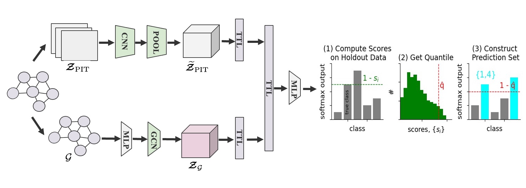
Combining persistence images of resolution from different filtration functions, we construct a multi-view topological representation, namely Persistent Image (PI) Tensor of dimension . We design the Multi-View Topological Convolutional Layer (MV-TCL) to (i) jointly extract and learn the latent topological features contained in the , (ii) leverage and preserve the multi-modal structure in the , and (iii) capture the structure in trainable weights (with fewer parameters). Firstly, hidden representations of the PI tensor are achieved through a combination of a CNN-based model and global pooling. Mathematically, we obtain a learnable topological tensor representation defined by
| (8) |
where is a CNN-based neural network, is a pooling layer that preserves the information of the input in a fixed-size representation (in general, we consider either global average pooling or global max pooling). Equation (8) provides two simple yet effective models to extract learnable topological features: (i) if only considering -dimensional topological features in , we can apply any CNN-based model to learn the latent feature of the ; (ii) if considering topological features with dimensions, we can additionally employ a global pooling layer over the latent feature and obtain an image-level feature. In this paper, we treat the resulting topological features in dimension 0 (connected components) and 1 (cycles) (i.e., ).
Graph Convolutional Layers.
Our third representation learning module is the Graph Convolutional Layer (GCL). It utilizes the graph structure of with its node feature matrix through the graph convolution operation and a multi-layer perceptron (MLP). Specifically, the designed graph convolution operation proceeds by multiplying the input of each layer with the -th power of the normalized adjacency matrix. The -th power operator contains statistics from the -th step of a random walk on the graph (in this study, we set to be 2), thus nodes can indirectly receive more information from farther nodes in the graph. Combined with a multi-layer perceptron (MLP), the representation learned at the -th layer is given by
| (9) |
where , , and is the corresponding degree matrix of , , is an MLP which has 2 layers with batch normalization, is the non-linear activation function, is a trainable weight of -th layer. Note that, to exploit multi-hop propagation information and increase efficiency, we can apply tensor decomposition (TD) techniques (e.g., tucker decomposition and canonical polyadic (CP) decomposition) over an aggregation of the outputs of all layers in Equation (9) to provide structure-aware representations of the input graph. Then, we obtain the final embedding by combining embeddings from the above modules, i.e., , where denotes the concatenation operation and represents the final output of the graph convolutional layer. Finally, we feed the final embedding into an MLP layer and use a differentiable classifier (here we use a softmax layer) to make graph classification.
Conditional Conformal Prediction.
Our proposed conditional uncertainty quantification algorithm aims at constructing the conditional prediction set for any graph with label , such that for any user-chosen error rate ,
| (10) |
where the probability measure is defined on the augmented data set and only with fixed (or from some local distribution).
Our idea is to only use the local (or similar) samples to obtain a prediction set. In particular, we define a local calibration set that contains data with similar graph structure, and assume . Then we can replace with to obtain a conditional prediction set. The detailed algorithm is described in the following.
After obtaining the trained model , we modify the original calibration steps to construct the conditional prediction set.
-
(1)
Calculate the non-conformity score:
where is the predicted probability of the -th subject having label . Similarly we define .
-
(2)
Define a conformal p-value that directly indicate a -level prediction set.
-
(3)
The prediction set can be defined as:
(11)
We will discuss the similarity measure between tensorized graphs in the sequel. The theoretical coverage is established in Proposition 1.
Proposition 1.
Assume and are exchangeable and independent with , the conformal prediction set obtained in this section satisfies (10) with conditional probability measure defined on the augmented data set and only with from the local distribution as .
Proof of Proposition 1: For notation simplicity, we index by and the target by . Let , and are i.i.d. given .
Order by , and as are continuous, we ignore the tie here. For , we have that . Given , there exists such that . Thus
Graph Similarity Measurement.
For a proper definition of a neighbourhood , the “similarity” can be measured in different ways. In this work, we consider two approaches: (i) topological similarity: Let and be persistence diagrams of two graphs and , respectively. Then we measure topological similarity among and as , where and is taken over all bijective maps between and , counting their multiplicities. In our analysis we use ; and (ii) similarity in the learned embedding space: We measure the graph similarity based on the similarity between graph-level embeddings from our CF-T2NN model. That is, the similarity between the two graphs is provided by their Euclidean distance in the CF-T2NN embedding space. We report classification performances of CF-T2NN under the above two graph similarity measures (see Table 2). Figure 1 illustrates our proposed CF-T2NN framework.
5 Experiments
The evaluation results on 10 datasets and the ablation study on 6 datasets are summarized in Tables 2 and 3 respectively.
5.1 Experiment Settings
Datasets.
We validate the Uncertainty Quantification (UQ) performance of the CF-T2NN model on graph classification tasks across two main types of datasets, chemical compounds and protein molecules. For the chemical compound dataset, we utilize four datasets, namely MUTAG, DHFR, BZR, and COX2 [64, 65], which comprise graphs representing chemical compounds, where nodes denote different atoms, and edges represent chemical bonds. For the molecular compound datasets, six datasets are used, including ENZYMES, PROTEINS, PTC_MR, PTC_MM, PTC_FM, and PTC_FR [66, 67, 68, 69, 65]. In molecular compound datasets, nodes represent amino acids, while edges denote the relationships or interactions between amino acids, such as physical bonds, spatial proximity, or functional interactions. For all graphs datasets, we adopt a split ratio of 0.5/0.2/0.21/0.09 for training, testing, calibration, and validation subsets, respectively. Table 1 summarizes the characteristics of all ten datasets used in our experiments.
| Dataset | # Graphs | Avg. | Avg. | # Class |
|---|---|---|---|---|
| ENZYMES | 600 | 32.63 | 62.14 | 6 |
| BZR | 405 | 35.75 | 38.35 | 2 |
| COX2 | 467 | 41.22 | 43.45 | 2 |
| DHFR | 756 | 42.43 | 44.54 | 2 |
| MUTAG | 188 | 17.93 | 19.79 | 2 |
| PROTEINS | 1113 | 39.06 | 72.82 | 2 |
| PTC_MR | 344 | 14.29 | 14.69 | 2 |
| PTC_MM | 336 | 13.97 | 14.32 | 2 |
| PTC_FM | 349 | 14.11 | 14.48 | 2 |
| PTC_FR | 351 | 14.56 | 15.00 | 2 |
Baselines. We compare our CF-T2NN with 7 state-of-the-art (SOTA) baselines including (i) Graph Convolutional Network (GCN) [70], (ii) Chebyshev GCN (ChebNet) [71], (iii) Graph Isomorphism Network (GIN) [72], (iv) GNNs with Differentiable Pooling (DiffPool) [73], (v) Self-attention Graph Pooling (SAGPool) [74], (vi) Topological Graph Neural Networks (GNN-TOGL) [59], and (vii) Simplicial Isomorphism Networ (SIN) [75].
Experimental Setup.
We run our experiments on a single NVIDIA Quadro RTX 8000 GPU card, which has up to 48GB of memory. To train the end-to-end CF-T2NN model, we use the Adam optimizer with a learning rate of 0.001. We use ReLU as the activation function across our CF-T2NN model, except Softmax for the MLP classifier output. For the resolution of the , we set the size to be . In our experiments, we consider different filtrations, i.e., degree-based, betweenness-based, closeness-based, and eigenvector-based filtrations. Depending on the dataset, we set batch sizes of either 16 or 32. The optimal number of hidden units for each layer in the graph convolution and MLPs are explored from the search space . The number of hidden units of TTL is 32. In addition, our CF-T2NN model has 3 layers in the graph convolution blocks and 2 layers in the MLPs, with a dropout rate of 0.5 for all datasets. We train our model for up to 100 epochs to make sure it is fully learned. To conduct the conditional conformal prediction, the number of neighbors of the -nearest neighbor method is set to either 80 or 100 (depending on the dataset), with a user-chosen error rate of 0.1. Our datasets and codes are available on https://www.dropbox.com/scl/fo/bi6x0hm83goxe7o0he5yr/h?rlkey=11sbequeppet9zp39blohjepa&dl=0.
5.2 Results
Table 2 shows the comparison of our proposed CF-T2NN with state-of-the-art baselines for graph classification on 10 datasets. We consider two variants of CF-T2NN, i.e., CF-T2NNT (i.e., based on topological similarity) and CF-T2NNE (i.e., based on similarity in the learned embedding space). The results indicate that our CF-T2NN always achieves the best performance, i.e., the average size of the prediction sets. Particularly, from Table 2, we observe that: (i) Compared to the GCN-based models (i.e., GCN and ChebNet), CF-T2NN improves upon the runner-up (i.e., ChebNet) by a margin of 19.12%, 26.02%, 36.72%, and 7.69% on COX2, DHFR, BZR, and MUTAG datasets respectively; (ii) Compared to the graph pooling methods (i.e., DiffPool and SAGPool), CF-T2NN yields an average relative gain of 13.36% on all datasets; and (iii) Compared to topology-based deep learning models (i.e., SIN and TOGL), CF-T2NN outperforms both models with a significant margin, especially on chemical graphs.
| Model | ENZYMES | COX2 | DHFR | BZR | MUTAG | PROTEINS | PTC_MR | PTC_MM | PTC_FM | PTC_FR |
|---|---|---|---|---|---|---|---|---|---|---|
| GCN [70] | 5.570.36 | 1.640.58 | 1.550.62 | 1.770.59 | 1.560.42 | 1.990.58 | 1.850.35 | 1.560.47 | 1.870.38 | 1.780.30 |
| ChebNet [71] | 5.640.29 | 1.620.48 | 1.550.64 | 1.750.55 | 1.540.49 | 1.960.57 | 1.870.36 | 1.590.50 | 1.850.32 | 1.710.35 |
| GIN [72] | 5.380.19 | 1.530.49 | 1.360.71 | 1.700.50 | 1.560.42 | 1.930.59 | 1.780.31 | 1.480.44 | 1.810.29 | 1.700.36 |
| DiffPool [73] | 5.210.24 | 1.650.47 | 1.470.57 | 1.700.40 | 1.580.52 | 1.910.48 | 1.830.35 | 1.480.49 | 1.860.31 | 1.720.44 |
| SAGPool [74] | 5.270.33 | 1.570.40 | 1.390.66 | 1.720.59 | 1.550.41 | 1.850.41 | 1.790.32 | 1.490.52 | 1.810.46 | 1.760.36 |
| SIN [75] | 5.730.32 | 1.500.43 | 1.440.77 | 1.640.56 | 1.530.57 | 1.690.43 | 1.800.35 | 1.490.45 | 1.850.32 | 1.720.31 |
| TOGL [59] | 5.060.25 | 1.510.58 | 1.360.74 | 1.650.50 | 1.490.45 | 1.580.47 | 1.860.37 | 1.520.45 | 1.820.40 | 1.740.30 |
| CF-T2NNT (ours) | 4.480.38 | 1.480.45 | 1.230.49 | 1.540.43 | 1.430.50 | 1.550.42 | 1.750.33 | 1.450.44 | 1.840.27 | 1.690.36 |
| CF-T2NNE (ours) | 4.610.82 | 1.360.47 | 1.280.48 | 1.280.48 | 1.440.50 | 1.560.41 | 1.690.36 | 1.450.45 | 1.720.35 | 1.660.38 |
| Architecture | ENZYMES | COX2 | MUTAG | PTC_MR | PTC_MM | PTC_FR |
|---|---|---|---|---|---|---|
| CF-T2NN w/o TTL | 4.530.43 | 1.370.48 | 1.480.48 | 1.780.32 | 1.480.48 | 1.810.29 |
| CF-T2NN | 4.480.38 | 1.360.47 | 1.430.50 | 1.690.36 | 1.450.44 | 1.660.38 |
5.3 Ablation Study
To better understand the importance of the tensor transformation layer (TTL) and the impact of uncertainty quantification (UQ) on performance across different architectures, we design ablation study experiments on the ENZYMES, COX2, MUTAG, PTC_MR, PTC_MM, and PTC_FR datasets. As shown in Table 3, CF-T2NN without the TTL module results in an average performance decline of over 5.04%, which highlights the critical role of learning the tensor structure of features. This ablation of TTL components not only leads to a larger prediction set size across all datasets but also underscores the efficacy of our uncertainty quantification method. Despite the performance drop, our UQ approach, particularly through conformal prediction, maintains strong statistical coverage of the prediction set results, ensuring reliability even in the absence of TTL. In summary, the ablation study not only confirms the integral role of TTL in the CF-T2NN model but also showcases the resilience of our UQ measures in providing dependable predictions.
6 Conclusion
In conclusion, our research has successfully addressed a significant gap in the field of GNNs by developing a novel model that robustly quantifies uncertainty, even in the presence of covariate shifts within graph-structured data. By integrating tensorized topological neural networks with an extended conformal prediction framework, we have introduced a method that not only adheres to statistical guarantees of coverage for conditional prediction sets but also respects the complex, multi-dimensional nature of graph data. This approach has proven effective across a diverse set of real-world datasets, showcasing its superiority over existing state-of-the-art methods in terms of reliability and precision. Our findings underscore the importance of considering domain shifts and the high-dimensional challenges inherent in graph data when quantifying uncertainty. This work sets a new standard for the application of GNNs in critical decision-making scenarios, offering a significant contribution to the fields of machine learning and graph analysis. We believe that our methodology will inspire further research into robust uncertainty quantification for GNNs and encourage the development of more reliable and interpretable models for complex systems analysis.
References
- [1] Jie Zhou, Ganqu Cui, Shengding Hu, Zhengyan Zhang, Cheng Yang, Zhiyuan Liu, Lifeng Wang, Changcheng Li, and Maosong Sun. Graph neural networks: A review of methods and applications. AI Open, 1:57–81, 2020.
- [2] Feng Xia, Ke Sun, Shuo Yu, Abdul Aziz, Liangtian Wan, Shirui Pan, and Huan Liu. Graph learning: A survey. IEEE Trans AI, 2(2):109–127, 2021.
- [3] Yijin Li, Han Zhou, Bangbang Yang, Ye Zhang, Zhaopeng Cui, Hujun Bao, and Guofeng Zhang. Graph-based asynchronous event processing for rapid object recognition. In Proceedings of the IEEE/CVF International Conference on Computer Vision, pages 934–943, 2021.
- [4] Xinjian Chen and Lingjiao Pan. A survey of graph cuts/graph search based medical image segmentation. IEEE reviews in biomedical engineering, 11:112–124, 2018.
- [5] Weizhu Qian, Dalin Zhang, Yan Zhao, Kai Zheng, and JQ James. Uncertainty quantification for traffic forecasting: A unified approach. In 2023 IEEE 39th International Conference on Data Engineering (ICDE), pages 992–1004. IEEE, 2023.
- [6] Hans Hao-Hsun Hsu, Yuesong Shen, Christian Tomani, and Daniel Cremers. What makes graph neural networks miscalibrated? Advances in Neural Information Processing Systems, 35:13775–13786, 2022.
- [7] Jize Zhang, Bhavya Kailkhura, and T Yong-Jin Han. Mix-n-match: Ensemble and compositional methods for uncertainty calibration in deep learning. In International conference on machine learning, pages 11117–11128. PMLR, 2020.
- [8] Balaji Lakshminarayanan, Alexander Pritzel, and Charles Blundell. Simple and scalable predictive uncertainty estimation using deep ensembles. Advances in neural information processing systems, 30, 2017.
- [9] Xiao Wang, Hongrui Liu, Chuan Shi, and Cheng Yang. Be confident! towards trustworthy graph neural networks via confidence calibration. Advances in Neural Information Processing Systems, 34:23768–23779, 2021.
- [10] Fangxin Wang, Yuqing Liu, Kay Liu, Yibo Wang, Sourav Medya, and Philip S. Yu. Uncertainty in graph neural networks: A survey, 2024.
- [11] Anastasios Nikolas Angelopoulos, Stephen Bates, Michael Jordan, and Jitendra Malik. Uncertainty sets for image classifiers using conformal prediction. In International Conference on Learning Representations, 2020.
- [12] Vladimir Vovk, Alexander Gammerman, and Glenn Shafer. Algorithmic learning in a random world, volume 29. Springer, 2005.
- [13] Kexin Huang, Ying Jin, Emmanuel Candès, and Jure Leskovec. Uncertainty quantification over graph with conformalized graph neural networks. 2023.
- [14] Soroush H. Zargarbashi, Simone Antonelli, and Aleksandar Bojchevski. Conformal prediction sets for graph neural networks. Proceedings of the 40th International Conference on Machine Learning, PMLR 202:12292-12318, 2023., 2023.
- [15] Ryan J Tibshirani, Rina Foygel Barber, Emmanuel Candes, and Aaditya Ramdas. Conformal prediction under covariate shift. Advances in neural information processing systems, 32, 2019.
- [16] Isaac Gibbs and Emmanuel Candes. Adaptive conformal inference under distribution shift. Advances in Neural Information Processing Systems, 34:1660–1672, 2021.
- [17] Jing Lei, Max G’Sell, Alessandro Rinaldo, Ryan J Tibshirani, and Larry Wasserman. Distribution-free predictive inference for regression. Journal of the American Statistical Association, 113(523):1094–1111, 2018.
- [18] Min-ge Xie and Zheshi Zheng. Homeostasis phenomenon in conformal prediction and predictive distribution functions. International Journal of Approximate Reasoning, 141:131–145, 2022.
- [19] Rina Foygel Barber, Emmanuel J Candes, Aaditya Ramdas, and Ryan J Tibshirani. The limits of distribution-free conditional predictive inference. Information and Inference: A Journal of the IMA, 10(2):455–482, 2021.
- [20] Jieli Shen, Regina Y Liu, and Min-ge Xie. i fusion: Individualized fusion learning. Journal of the American Statistical Association, 115(531):1251–1267, 2020.
- [21] Chencheng Cai, Rong Chen, and Min-ge Xie. Individualized group learning. Journal of the American Statistical Association, 118(541):622–638, 2023.
- [22] Hua Zhou, Lexin Li, and Hongtu Zhu. Tensor regression with applications in neuroimaging data analysis. Journal of the American Statistical Association, 108(502):540–552, 2013.
- [23] Elynn Y Chen, Ruey S Tsay, and Rong Chen. Constrained factor models for high-dimensional matrix-variate time series. Journal of the American Statistical Association, 2020.
- [24] Xialu Liu and Elynn Chen. Identification and estimation of threshold matrix-variate factor models. Scandinavian Journal of Statistics, 2022.
- [25] Elynn Chen and Rong Chen. Modeling dynamic transport network with matrix factor models: with an application to international trade flow. Journal of Data Science, 2022.
- [26] Xuan Bi, Annie Qu, and Xiaotong Shen. Multilayer tensor factorization with applications to recommender systems. The Annals of Statistics, 46(6B):3308–3333, 2018.
- [27] Elynn Chen, Xin Yun, Rong Chen, and Qiwei Yao. Modeling multivariate spatial-temporal data with latent low-dimensional dynamics. arXiv preprint arXiv:2002.01305, 2020.
- [28] Elynn Chen, Dong Xia, Chencheng Cai, and Jianqing Fan. Semi-parametric tensor factor analysis by iteratively projected singular value decomposition. Journal of the Royal Statistical Society Series B: Statistical Methodology, page qkae001, 2024.
- [29] Elynn Chen, Xi Chen, Wenbo Jing, and Yichen Zhang. Distributed tensor principal component analysis. arXiv preprint arXiv:2405.11681, 2024.
- [30] Anru Zhang and Dong Xia. Tensor svd: Statistical and computational limits. IEEE Transactions on Information Theory, 64(11):7311–7338, 2018.
- [31] Lexin Li and Xin Zhang. Parsimonious tensor response regression. Journal of the American Statistical Association, 112(519):1131–1146, 2017.
- [32] Dong Xia, Anru R. Zhang, and Yuchen Zhou. Inference for low-rank tensors—no need to debias. The Annals of Statistics, 50(2):1220–1245, 2022.
- [33] Elynn Chen, Jianqing Fan, and Xiaonan Zhu. Factor augmented matrix regression. arXiv preprint arXiv:2405.17744, 2024.
- [34] W. W. Sun and L. Li. Dynamic tensor clustering. Journal of the American Statistical Association, 114(528):1894–1907, 2019.
- [35] Qing Mai, Xin Zhang, Yuqing Pan, and Kai Deng. A doubly enhanced EM algorithm for model-based tensor clustering. Journal of the American Statistical Association, pages 1–15, 2021.
- [36] Yuetian Luo and Anru R. Zhang. Tensor clustering with planted structures: Statistical optimality and computational limits. The Annals of Statistics, 50(1):584–613, 2022.
- [37] Zhifeng Hao, Lifang He, Bingqian Chen, and Xiaowei Yang. A linear support higher-order tensor machine for classification. IEEE Transactions on Image Processing, 22(7):2911–2920, 2013.
- [38] Xian Guo, Xin Huang, Lefei Zhang, Liangpei Zhang, Antonio Plaza, and Jón Atli Benediktsson. Support tensor machines for classification of hyperspectral remote sensing imagery. IEEE Transactions on Geoscience and Remote Sensing, 54(6):3248–3264, 2016.
- [39] Elynn Chen, Yuefeng Han, and Jiayu Li. High-dimensional tensor classification with cp low-rank discriminant structure. arXiv preprint arXiv:2409.14397, 2024.
- [40] Kishan Wimalawarne, Ryota Tomioka, and Masashi Sugiyama. Theoretical and experimental analyses of tensor-based regression and classification. Neural Computation, 28(4):686–715, 2016.
- [41] Jean Kossaifi, Zachary C Lipton, Arinbjorn Kolbeinsson, Aran Khanna, Tommaso Furlanello, and Anima Anandkumar. Tensor regression networks. Journal of Machine Learning Research, 21(123):1–21, 2020.
- [42] Tao Wen, Elynn Chen, and Yuzhou Chen. Tensor-view topological graph neural network. In International Conference on Artificial Intelligence and Statistics, 2024, València SPAIN, 2024.
- [43] Nadav Cohen, Or Sharir, and Amnon Shashua. On the expressive power of deep learning: A tensor analysis. In Conference on Learning Theory, pages 698–728, 2016.
- [44] Jean Kossaifi, Aran Khanna, Zachary C. Lipton, Tommaso Furlanello, and Anima Anandkumar. Tensor contraction layers for parsimonious deep nets. CVPR, pages 1940–1946, 2017.
- [45] Jean Kossaifi, Zachary C. Lipton, Arinbjorn Kolbeinsson, Aran Khanna, Tommaso Furlanello, and Anima Anandkumar. Tensor regression networks. JMLR, 21:1–21, 2020.
- [46] Yao Lei Xu, Kriton Konstantinidis, and Danilo P Mandic. Graph tensor networks: An intuitive framework for designing large-scale neural learning systems on multiple domains. arXiv preprint arXiv:2303.13565, 2023.
- [47] H. Edelsbrunner, D. Letscher, and A. Zomorodian. Topological persistence and simplification. In FOCS, pages 454–463, 2000.
- [48] A. Zomorodian and G. Carlsson. Computing persistent homology. Discrete & Computational Geometry, 33(2):249–274, 2005.
- [49] Nina Otter, Mason A Porter, Ulrike Tillmann, Peter Grindrod, and Heather A Harrington. A roadmap for the computation of persistent homology. EPJ Data Science, 6:1–38, 2017.
- [50] Mehmet E Aktas, Esra Akbas, and Ahmed El Fatmaoui. Persistence homology of networks: methods and applications. Applied Network Science, 4(1):1–28, 2019.
- [51] Chi Seng Pun, Kelin Xia, and Si Xian Lee. Persistent-homology-based machine learning and its applications–a survey. arXiv preprint arXiv:1811.00252, 2018.
- [52] Christoph Hofer, Roland Kwitt, Marc Niethammer, and Andreas Uhl. Deep learning with topological signatures. In Advances in Neural Information Processing Systems, pages 1634–1644, 2017.
- [53] Thomas Bonis, Maks Ovsjanikov, Steve Oudot, and Frédéric Chazal. Persistence-based pooling for shape pose recognition. In Computational Topology in Image Context: 6th International Workshop, CTIC 2016, Marseille, France, June 15-17, 2016, Proceedings 6, pages 19–29. Springer, 2016.
- [54] Zixuan Cang, Lin Mu, and Guo-Wei Wei. Representability of algebraic topology for biomolecules in machine learning based scoring and virtual screening. PLoS computational biology, 14(1):e1005929, 2018.
- [55] Yuzhou Chen and Yulia R Gel. Topological pooling on graphs. In Proceedings of the AAAI Conference on Artificial Intelligence, volume 37, pages 7096–7103, 2023.
- [56] Yuzhou Chen, Ignacio Segovia, and Yulia R Gel. Z-gcnets: Time zigzags at graph convolutional networks for time series forecasting. In International Conference on Machine Learning, pages 1684–1694. PMLR, 2021.
- [57] Mathieu Carriere, Frédéric Chazal, Inria Saclay Datashape, Yuichi Ike, Théo Lacombe, Martin Royer, and Yuhei Umeda. Perslay: A simple and versatile neural network layer for persistence diagrams. stat, 1050:5, 2019.
- [58] Manzil Zaheer, Satwik Kottur, Siamak Ravanbakhsh, Barnabas Poczos, Russ R Salakhutdinov, and Alexander J Smola. Deep sets. Advances in neural information processing systems, 30, 2017.
- [59] Max Horn, Edward De Brouwer, Michael Moor, Yves Moreau, Bastian Rieck, and Karsten Borgwardt. Topological graph neural networks. In International Conference on Learning Representations.
- [60] Yuzhou Chen, Yulia Gel, and H Vincent Poor. Time-conditioned dances with simplicial complexes: Zigzag filtration curve based supra-hodge convolution networks for time-series forecasting. Advances in Neural Information Processing Systems, 35:8940–8953, 2022.
- [61] Gunnar Carlsson and Mikael Vejdemo-Johansson. Topological Data Analysis with Applications. Cambridge University Press, 2021.
- [62] Henry Adams, Tegan Emerson, Michael Kirby, Rachel Neville, Chris Peterson, Patrick Shipman, Sofya Chepushtanova, Eric Hanson, Francis Motta, and Lori Ziegelmeier. Persistence images: A stable vector representation of persistent homology. Journal of Machine Learning Research, 18, 2017.
- [63] Ivan V Oseledets. Tensor-train decomposition. SIAM Journal on Scientific Computing, 33(5):2295–2317, 2011.
- [64] Jeffrey J Sutherland, Lee A O’brien, and Donald F Weaver. Spline-fitting with a genetic algorithm: A method for developing classification structure- activity relationships. Journal of Chemical Information and Computer Sciences, 43(6):1906–1915, 2003.
- [65] Nils Kriege and Petra Mutzel. Subgraph matching kernels for attributed graphs. In Proceedings of the International Conference on Machine Learning, pages 291–298, 2012.
- [66] Christoph Helma, Ross D. King, Stefan Kramer, and Ashwin Srinivasan. The predictive toxicology challenge 2000–2001. Bioinformatics, 17(1):107–108, 2001.
- [67] Ida Schomburg, Antje Chang, Christian Ebeling, Marion Gremse, Christian Heldt, Gregor Huhn, and Dietmar Schomburg. Brenda, the enzyme database: updates and major new developments. Nucleic Acids Research, 32(suppl_1):D431–D433, 2004.
- [68] Paul D Dobson and Andrew J Doig. Distinguishing enzyme structures from non-enzymes without alignments. Journal of Molecular Biology, 330(4):771–783, 2003.
- [69] Karsten M Borgwardt, Cheng Soon Ong, Stefan Schönauer, SVN Vishwanathan, Alex J Smola, and Hans-Peter Kriegel. Protein function prediction via graph kernels. Bioinformatics, 21:i47–i56, 2005.
- [70] Thomas N Kipf and Max Welling. Semi-supervised classification with graph convolutional networks. arXiv preprint arXiv:1609.02907, 2016.
- [71] Michaël Defferrard, Xavier Bresson, and Pierre Vandergheynst. Convolutional neural networks on graphs with fast localized spectral filtering. Advances in neural information processing systems, 29, 2016.
- [72] Keyulu Xu, Weihua Hu, Jure Leskovec, and Stefanie Jegelka. How powerful are graph neural networks? In Proceedings of International Conference on Learning Representations, 2018.
- [73] Zhitao Ying, Jiaxuan You, Christopher Morris, Xiang Ren, Will Hamilton, and Jure Leskovec. Hierarchical graph representation learning with differentiable pooling. In Advances in Neural Information Processing Systems, volume 31, 2018.
- [74] Junhyun Lee, Inyeop Lee, and Jaewoo Kang. Self-attention graph pooling. In Proceedings of the International Conference on Machine Learning, pages 3734–3743, 2019.
- [75] C. Bodnar, F. Frasca, Y. G. Wang, N. Otter, G. Montúfar, P. Lio, and M. Bronstein. Weisfeiler and Lehman go topological: Message passing simplicial networks. In Proceedings of the International Conference on Machine Learning, 2021.