Chasing Random – Investigating the ‟Gains˝ achieved through Instruction Selection Strategies at Scale

Abstract

Prior work Zhou et al. (2023a) has shown that language models can be tuned to follow user instructions using only a small set of high-quality instructions. This has accelerated the development of methods that filter a large, noisy instruction-tuning datasets down to high-quality subset which works just as well. However, typically, the performance of these methods is not demonstrated across a uniform experimental setup and thus their generalization capabilities are not well established. In this work, we analyze popular selection strategies across different source datasets, selection budgets and evaluation benchmarks: Our results indicate that selection strategies generalize poorly, often failing to consistently outperform even random baselines. We also analyze the cost-performance trade-offs of using data selection. Our findings reveal that data selection can often exceed the cost of fine-tuning on the full dataset, yielding only marginal—and sometimes no gains compared to tuning on the full dataset or a random subset.

Chasing Random – Investigating the ‟Gains˝ achieved through Instruction Selection Strategies at Scale

Harshita Diddee¹  Daphne Ippolito^{1,2 1}Carnegie Mellon University ² Google Deepmind {hdiddee,dippolit}@andrew.cmu.edu

1 Introduction

Instruction fine-tuning is often considered a crucial step in training large language models, LLMs, to effectively meet the needs of users. By training LLMs over tens of thousands instruction-response tuples that highlight user preferences, models can demonstrate instruction-following capabilities which position them as useful tools for a wide variety of tasks. There has been a rapid increase in the development of instruction selection strategies Qin et al. (2024b); Wang et al. (2024) to curate a subset of high-quality instructions to train competitive instruction following models more efficiently.

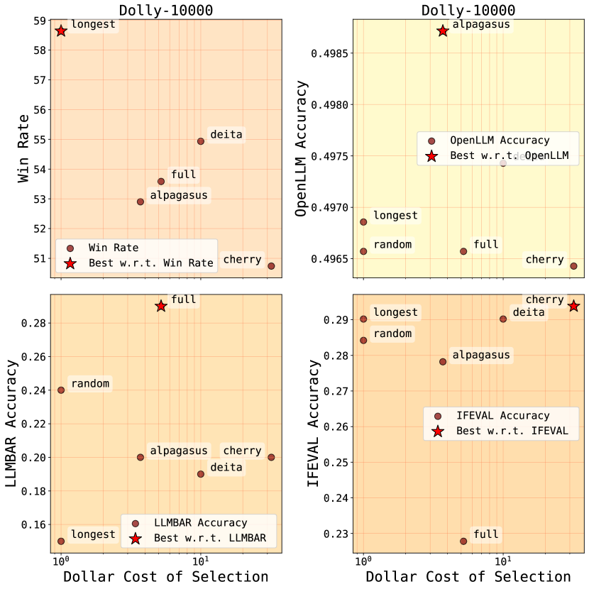
Figure 1: Selection Cost Versus Performance on different benchmarks when selecting 10000 samples from Dolly Conover et al. (2023): Upper Left Region (low cost, high performance) is ideal. Key Takeaways are: (a) Random baselines are reasonably competitive whilst incurring the least cost (b) Depending on the evaluation metric, the best strategy varies significantly with the setup ($\star$indicates best selection strategy on the benchmark).

The experimental setups of general-purpose instruction data selection can be very varied Qin et al. (2024b); Unlike task-specific data selection, they are not geared towards optimizing performance for some specific goal Xie et al. (2023a). Therefore, their utility is strongly tied to their generalization beyond a few limited setups endorsed by their designers.

Measuring this generalization is hard for several reasons. Firstly, proposed strategies are often applied across arbitrary experimental setups including different source datasets, selection budgets and testing benchmarks. Additionally, since there isn’t a single set of behaviors expected of instruction tuned models, it is unclear performance gained through selection on one instruction-following benchmark will induce correlated gains on other instruction-following benchmarks. Finally, the time and resources necessitated by a selection strategy vary significantly. While strategies like Chen et al. (2023) can directly incur dollar-cost through their dependence on API-accessible commercial large language model APIs, others like Li et al. (2023a); Liu et al. (2023) design selection methods that involve finetuning or inferencing on LLMs, thus mandating a GPU-reliant infrastructural cost.

Contribution: In this work, we carry out an exhaustive investigation for over 60 experimental configurations across 4 evaluation benchmarks each to provide evidence for the following findings (a) Instruction Selection Strategies don’t generalize to reasonably similar experimental configurations. Consequently, no selection strategy beats random selection consistently. (b) Competence in General Purpose Instruction Following is a subjective goal and hence, comparing selection strategies on different facets of this goal can produce contradictory trends. (c) Many strategies scale poorly as the budget of selection increases: Incurred selection costs can often overshoot the cost of training with the entire dataset and do not give consistently high gains over random selection carried out at negligible cost.

We argue that the lack of generality and consistent performance over a naive baseline makes it difficult to use existing example selection strategies in the wild: if selection through a strategy is not consistently cost-effective over a naive form of subsampling (random-sampling) across reasonably similar experimental configurations, it is unclear if selection is an advantageous step in the process of training competitive LLMs.

2 Literature Review

We focus on general-purpose instruction selection methods, which aim to equip models to follow user queries that aren’t specific to a fixed task, capability or domain Wang et al. (2024).Such methods involve strategies including rule-based metrics Cao et al. (2023), length Zhao et al. (2024), diversity Liu et al. (2023) and model derived uncertainity measurements Li et al. (2023a) to subsample large instruction tuning datasets. They sit in contrast to task-specific data selection strategies which optimize for performance on a known test distribution or task specification Xia et al. (2024); Xie et al. (2023b); Pan et al. (2024).

Due to broad definition of instructing following, experimental setups for such work can show significant variation: While some adopt source distiributions of varying origins Zhou et al. (2023a); Li et al. (2024); Shen (2024), some even synthetically augment subsets of data during their selection process Liu et al. (2023). Similarly, the selection budget applied on these datasets can vary from anywhere between a mere 200 samples Wei et al. (2023) to 15K Du et al. (2023); Xia et al. (2024). We summarize some of the most popular choices in Table 1 and utilize these for our experiments.
A few methods also Mekala et al. (2024); Xia et al. (2024) acknowledge and accordingly attempt to address the relatively high cost of selection by either exploring the use of cheaper proxies like smaller models, low-rank approximations or adopting sequential pipelines Ge et al. (2024) to make instruction data selection more efficient. Finally, work like Liu et al. (2024); Wang et al. (2024) have highlighted the concerns in comparing between the performance of instruction selection strategies. Through a unified comparison based on efficiency and feasibility, Liu et al. (2024) provide strong evidence that the comparison between instruction selection strategies needs to be more holistic. Distinctive from this work though, their evaluation does not focus on a comparison including random baselines.

Source Distribution	Authorship	Number of Samples	Brief Description
FLAN  Longpre et al. (2023)	Automatic	88k	Includes Flan 2021, P3, Super-Natural Instructions among other datasets.
Dolly  Conover et al. (2023)	Human	15k	Instruction-responses crafted by Databricks employees.
Evol  Xu et al. (2023)	LLM	196k	Modifying seed instructions using ChatGPT.
Alpaca Taori et al. (2023)	LLM	52k	ChatGPT driven generation with Self-Instruct’s pipeline.
Evaluation Setup	Number of Samples	Metric	Brief Description
IFEval Zhou et al. (2023b)	500	Instruct, Prompt Level Accuracy	Instructions have verifiable prompts to check if model fulfills all prompts in an instruction.
AlpacaEval  Li et al. (2023b)	805	Length Controlled Win Rate	Judges LLM responses by an automatic annotator with high human-correlation.
LLMBAR  Zeng et al. (2023)	100 (Natural Set)	Accuracy	Checks model preference over instruction responses to check if a model identifies faithful responses.
OpenLLM  Gao et al. (2023)	Task-Specific	Accuracy	MMLU, ARC-Easy, ARC-Challenge, WinoGrande, TruthfulQA, HellaSwag

Table 1: A brief overview of the source distributions we investigate and the Evaluation Setups we consider.

3 Experimental Setup

In this section, we briefly describe our source datasets, the selection strategies we study and our evaluation setup.

3.1 Source Datasets and Evaluation Setups

Table 1 provides a concise description of all our datasets and evaluation benchmarks. For FLAN, as a precaution against including disproportionately high representations towards tasks that are overly-represented in the original composition, we curate a smaller subset of FLAN, by limiting the datapoints sampled per task to 50 for our evaluation. The resulting dataset contains 88K examples and we refer to this version as FLAN. For AlpacaEval, we use a fixed randomly sampled subset of 300 samples to reduce the cost overhead of our evaluations. We use the default recommended annotator configuration using GPT-4-Turbo.

3.2 Selection Strategies

Alpagasus ($S_{\text{alpagasus}}$)

Chen et al. (2023) use GPT-3.5 as scorer (between 1-5) to score samples from Alpaca and include the highest scoring samples.

Longest ($S_{\text{longest}}$)

Zhao et al. (2024) include the instructions with the longest responses.

Cherry ($S_{\text{cherry}}$)

Li et al. (2023a) use a sequential approach of selecting instructions: they apply k-means clustering to the last hidden state embeddings of all instruction in a source dataset to get a set of 1000 instructions (100 clusters and 10 samples per cluster). Then, they use this subset of instructions to finetune a model, referred to as the pre-experienced model. Finally, this model scores each sample with an Instruction Difficulty or IFD and the highest scoring samples are included in the selected subset.

DEITA ($S_{\text{deita}}$)

Liu et al. (2023) train a scorer akin to Alpagasus to first score the entire dataset cheaply and then, rather than choosing the entire budget of instructions in one shot - iteratively construct the selected subset by checking the similarity of a candidate instruction to the current pool of instructions.

Uniform Random ($S_{\text{random}}$)

This is the naivest form of sampling and acts as our baseline. We report numbers with error bars for trials across 3 such random seeds. We also resample for any random subset that ends up having more than 30% overlap with the data sampled with any strategy for all datasets expect dolly (due to Dolly’s limited size, a maximum overlap of about 50% is possible only for the highest budget 10000).

Strict Random ($S_{\text{strictrandom}}$)

We also create a special variant of our random-baselines called the "strictrandom" baselines which is created by sampling from the dataset after removing all the target instructions that have been deemed high-quality by any of the selection strategies. In practice, the strictrandom baselines can also be considered as sampling data from the complement set of all strategies’ "high-quality" subsets of budget 10000.

Full Dataset:

The entire dataset is used to train the model. Note that we include this variant without tuning optimally for each dataset and include this only to compare the gains that can be naively procured by avoiding selection altogether.

3.3 Base Model

We use the LLaMa-7B Touvron et al. (2023) for all our experiments.This model’s choice is dictated by it’s use as a common choice for demonstrating and ablating the performance of the instruction selection strategies that we study (Table 2 Qin et al. (2024b)). We provide all details of the 3 hyperparameter sets we test in the Appendix A.1).

4 Results

In this section, we present evidence supporting our conclusions on the brittle generalization of instruction selection strategies (§4.1 and §4.2) as well as the negative utility of expending cost on data selection §4.3.

4.1 Most Strategies Fail to Beat Random Sampling Consistently

In the space of instruction data selection, it is very common to show that $M_{\text{selected}}$ outperform $M_{\text{full-dataset}}$ by over 50% (i.e., an LLM judge prefers the outputs of the $M_{\text{selected}}$ more than the $M_{\text{full-dataset}}$). We modify this experimental setup to perform these comparisons between the $M_{\text{random}}$ and $M_{\text{selected}}$ on AlpacaEval. Specifically, for each model in $M_{\text{selected}}$, we pair the output of the $M_{\text{selected}}$ with a randomly chosen inference generated by a random baseline from the $M_{\text{random}}$ trained for the same budget and dataset. We then compute the Mean-Adjusted Win-Rate by taking the signed difference between the win-rate of the $M_{\text{selected}}$ from 50%. Our results across two budgets are summarized in Figure 2.

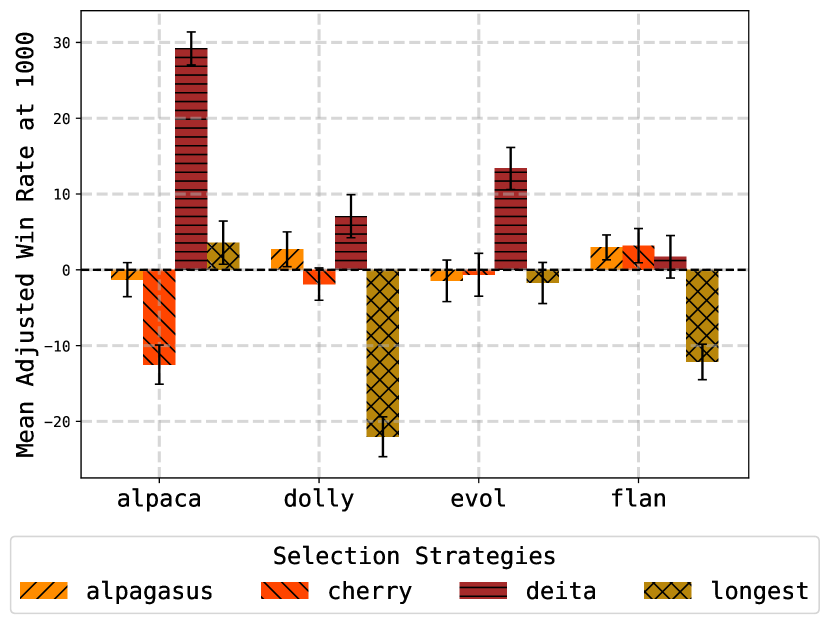
(a)

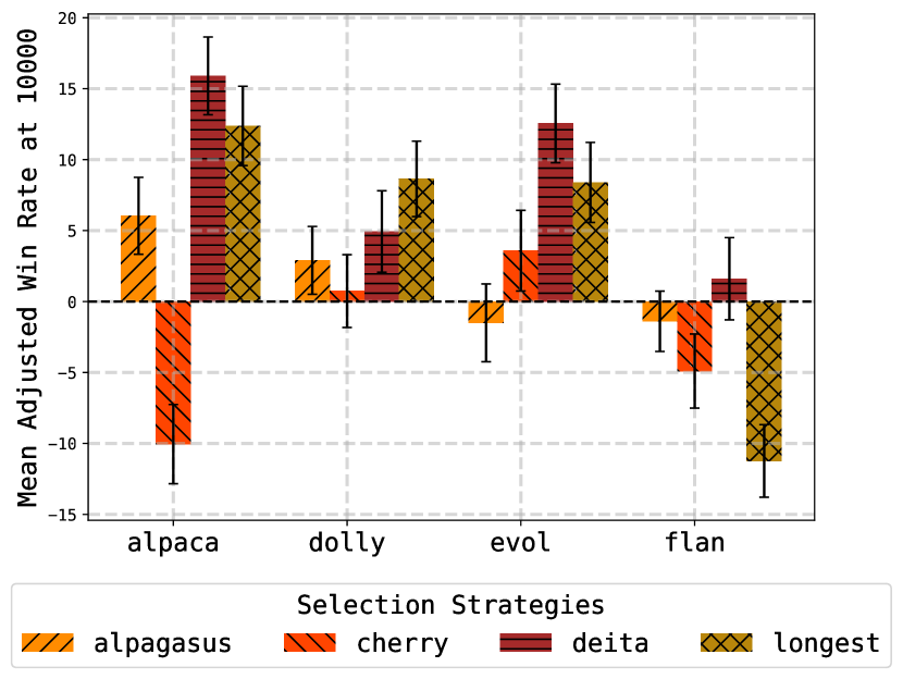
(b)

Figure 2: Mean Adjusted Win Rates on AlpacaEval for budgets (a) 1000 (b) 10000. A bar along the negative y-axis indicates that the $M_{\text{random}}$ responses are preferred more than 50% of the time by GPT-4. No strategy except $S_{\text{deita}}$ beats random baselines consistently. No strategy shows consistent performance trends across budgets as well (Section §4.1) for more details.

Findings on AlpacaEval No strategy except $S_{\text{deita}}$, consistently dominates over the $M_{\text{random}}$ across all experimental configurations. To illustrate the practical implications of this observation, consider an NLP practitioner who intends to apply data selection on the Dolly dataset with a budget of 10,000 samples. They evaluate the performance of various selection strategies on Dolly at a smaller budget of 5,000 samples and conclude that $S_{\text{cherry}}$ is the most effective strategy (Figure 2). However, when this strategy is applied and empirically tested at the intended budget of 10,000 samples, the results are the opposite: $S_{\text{cherry}}$ delivers the lowest performance among all strategies (Figure 2). While we give an example with $S_{\text{cherry}}$, it is reasonable to assume that other strategies experience similar inflection points in their performance with the change in budget. For example, even though $S_{\text{deita}}$consistently outperforms random in this evaluation, it loses nearly 15% of its dominance over $M_{\text{random}}$ at budget 10000 (when scaled from 5000) indicating the potential for an inflection point in performance for some larger budget.

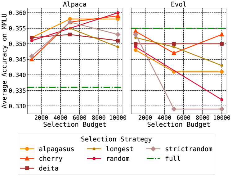
(a) Performance Trends According to MMLU

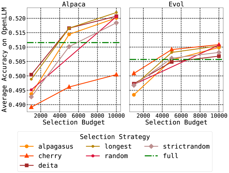
(b) Performance Trends According to Average Performance on Subset of OpenLLM

Figure 3: There is a stark difference between the performance trends of selection strategies depending upon what subset of OpenLLM tasks are chosen for evaluation. $S_{\text{random}}$ is the worst performing strategy across all datasets when performance is gauged on MMLU, while $S_{\text{random}}$ shows competitive performance as more tasks from OpenLLM are considered. Details in §4.1 and 9(b).

.

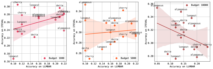
Figure 4: Mean Instruct-Level Accuracy of $M_{\text{selected}}$ on IFEval versus Win-Rate on AlpacaEval: The correlation between Win-Rate and IFEval is entirely non-existent or weakly correlated at best. As budget increases these also appear to diverge: as performance drops on Win-Rate as IFEval accuracy improves. (§4.2 for further details.)

Findings with OpenLLM

To corroborate this trend, we evaluate $M_{\text{selected}}$ with $M_{\text{random}}$ on OpenLLM. In Figure 3(b), we demonstrate the performance of $M_{\text{selected}}$ across different budgets on both (a) MMLU (the only task evaluated by Chen et al. (2023)) and (b) average performance on 7 tasks from OpenLLM (the largest union of tasks considered by Zhao et al. (2024); Li et al. (2023a)). Not surprisingly, we find extreme divergence in the observed performance trends of selection strategies depending upon which setup is adopted: While $S_{\text{random}}$ subsampling performs the worst by a significant margin against all selection strategies when evaluated using only MMLU (Fig 3(b) (a)), it performs far more competitively when more tasks from OpenLLM are considered (Fig 3(b) (b)), especially performing competitively at larger budgets. Note that this setup only highlights the difficulty arising out of using a non-standard subset of evaluation tasks and does not question if its even appropriate to consider any of these tasks as a reasonable indicator of a model’s instruction following capabilities. MMLU, for example, has been shown to demonstrate several contextual limitations Gema et al. (2024) in addition to being a multiple choice format task which significantly deviates from the traditional long-form generation format of instruction following benchmarks. Hence, it would not be too unreasonable to assume that it may not be a sufficiently aligned choice for demonstrating that a $M_{\text{selected}}$ demonstrates instruction following capabilities in the first place.

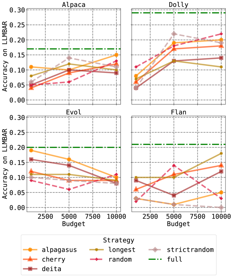
Figure 5: Performance on LLMBAR: Both $M_{\text{random}}$ and $M_{\text{selected}}$ consistently underperform $M_{\text{full-dataset}}$.

4.2 Measuring Instruction Following for $M_{\text{selected}}$produces contradictory trends

Measuring instruction following capabilities is generally more complex than task-specific accuracy evaluation as instruction following models are expected to demonstrate a wide range of capabilities Lou et al. (2024). Consequently, the subjectivity in the coverage of topics and the performance ranges of each instruction following benchmark can further influence our estimates of a selection strategy’s performance. Recently, an emerging class of benchmarks recommend evaluating models with instructions which have more objective requirements Qin et al. (2024a); Zhou et al. (2023b). Accordingly, we conduct an evaluation of $M_{\text{selected}}$ on another popular instruction following benchmark that complies with this format, IFEval Zhou et al. (2023b). IFEval defines its own metrics, prompt-level and instruction-level accuracy, to measure how well a model response covers all the requirements delineated by each prompts and ultimately the test instruction. As in our previous evaluation with AlpacaEval and OpenLLM, we compare the performance of $M_{\text{selected}}$ and $M_{\text{random}}$ on this benchmark.

Findings from IFEval

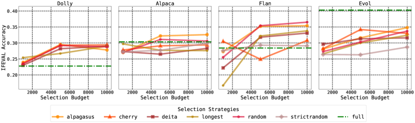
Figure 10: Performance Comparison between $M_{\text{random}}$and $M_{\text{selected}}$on IFEVAL: We report the average of all random runs (both random and strict random) for a particular configuration in any result.

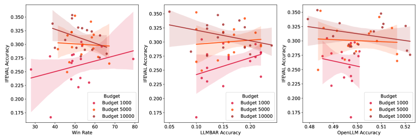
Figure 11: Correlation between Benchmarks: All benchmarks show poor correlation, especially at larger budgets (almost negatively correlated performances)

We include complete results on IFEval in the Appendix (Figure 10), where we observe similarly competitive performance from $M_{\text{random}}$; Here, we highlight another interesting observation derived through this benchmark: In Figure 4, we show the correlation between the Win-Rates for $M_{\text{selected}}$ and their IFEval accuracy 4. The performance trends on both benchmarks appear very weakly correlated for our lowest budget, and show almost negative correlation after scaling $M_{\text{selected}}$ to the larget budget. This is particularly concerning as both benchmarks are widely used as indicators of instruction following capabilities and hence, at least by definition it is hard to pick the conclusions of one over the other. The practical implication of this correlation is observed when these setups disagree on what the most appropriate selection strategy for a setup is. In this case for instance, we see that a lower budget (Figure 4(, we can claim with reasonable confidence that $S_{\text{deita}}$ would give high performance across both benchmarks but as budget scales the trade-off between the performances on both benchmarks increases significantly making it hard to conclude which strategy has higher utility. We also observe similarly poor correlations between the performance trends of selection strategies when we do a pair wise comparison between other studied benchmarks like OpenLLM and LLMBAR (Figure 11).

To demonstrate this more concretely, we conduct a final evaluation on another instruction following benchmark, LLMBAR.

Findings from LLMBAR

In Figure 5, we observe that both $M_{\text{selected}}$ and $M_{\text{random}}$ perform poorly on this benchmark. Interestingly, unlike all other benchmarks we study where $M_{\text{full-dataset}}$ are either comparable in performance or even underperform $M_{\text{selected}}$, on LLMBAR we clearly see consistent performance improvement when the model is trained on the entire data. This result, hence, sits in complete contrast to all other benchmark evaluations as it exposes another facet of evaluation where selection is not advantageous at all.

4.3 Cost of Instruction Data Selection is Non-Trivial when compared to the cost of Tuning on the Entire Data

Dataset Samples (as multiples of 1k) Alpagasus Cherry DEITA Entire Dataset Costing Categories API Inference Cost (USD) Rent Time (min) Rent Cost (USD) Rent Time (min) Rent Cost (USD) Rent Time (min) Rent Cost (USD) EVOL 200 50 3290 427 1000 130 1620 216 ALPACA 52 12.66 855 111.15 260 33.8 120 15.6 DOLLY 15 3.7 246.75 32.07 75 9.975 40 5.2 FLAN 88 21.46 1447.6 188.2 440 57.2 220 28.6

Table 2: Random and Longest incur negligible time and compute cost on our setups and hence, they are not included here. For all other strategies, the effective cost of data selection is non-trivial in comparison to training on the full-dataset. In three out of four strategies, it is possible to overshoot the cost of finetuning on the full dataset.

A strong motivation for designing instruction selection strategies, and more broadly, data selection strategies draws from the need to train competitive models efficiently, both in terms of time and resource consumption. While the advantages towards this goal are more explicitly observed when source datasets are very large (pretraining datasets of the order of billions of tokens), instruction tuning datasets are typically much smaller in magnitude and thus the efficiency gains of selection can be less obvious to gauge. Accordingly, we evaluate if the proposed selection strategies consistently provide this intended benefit by comparing the effective cost of selection against the performance of $M_{\text{selected}}$ and $M_{\text{full-dataset}}$.

Setup We compute the Cost of Selection as a product of the per-hour cost to user for renting a fixed compute infrastructure and the wall clock run time for running the selection for that strategy end-end. §B describes the full details of this computation including the wall clock time of running each selection (Table 6), while the total cost to user in summarized in Table 2. In Figure 6, we plot the cost of selection per dataset compared to the performances of $M_{\text{selected}}$ on IFEVAL (all budgets are included in §B.3 in the Appendix).

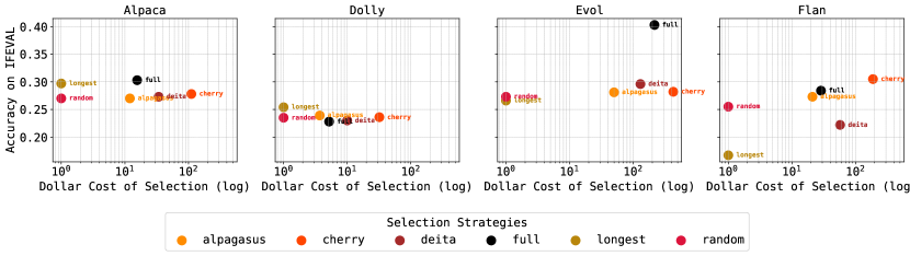
Figure 6: Cost Versus Performance Trade-Off at Selection Budget of 1000: Rather than reporting the average performance of random - we report the lowest performance amongst all our random trials to give the most pessimistic estimate of the performance of our random baseline.

Finding The effective cost of selecting data can often overshoot the cost of finetuning $M_{\text{full-dataset}}$ in some cases and the gains achieved through selection are marginal in comparison to the additional cost expended at carrying out the selection. While one potential cause of this could be the lack of more aggressive strategy-specific hyperparameter tuning, that is impractical for multiple reasons; For one, hyperparameter tuning in this space involves tuning for strategy dependent parameters such as the similarity threshold, $\lambda$ in $S_{\text{deita}}$, the number of pre-experienced samples in $S_{\text{cherry}}$, etc. in addition to traditional model training parameters like learning rate, scheduler and batch size. Jointly optimizing for both these class of hyperparameters can significantly bloat the set of combinations to explore for hyperparameter optimization thus significantly increasing the cost of tuning. Secondly, under a practical setup where an NLP pracitioner expects to choose the best selection strategy amongst several candidate strategies, a hyperparameter sweep for each candidate strategy would mandate tuning all the strategies being examined. From 2, this would imply summing the cost estimates across any row. We can clearly see that such an estimate would quickly overshoot the cost of full finetuning for any strategy.

One interesting and consistent observation from this cost-benefit analysis is the surprising performance gain shown by $M_{\text{selected}}$ over $M_{\text{full-dataset}}$. Both, $M_{\text{selected}}$ and $M_{\text{random}}$ often beat the $M_{\text{full-dataset}}$ across several experimental configurations. While some of these gains may be attributed to the lack of hyperparameter tuning for $M_{\text{full-dataset}}$, supporting evidence from literature in the space of instruction data selection (Qin et al. (2024b); Zhou et al. (2023a); Zhao et al. (2024); Ge et al. (2024) does imply that training on selected data can be beneficial (even though not necessarily cost effective). Empirically, this is also visible from the performance of our $S_{\text{strictrandom}}$ baselines: through the majority of our evaluation, the $S_{\text{strictrandom}}$ baselines underperform all other strategies indicating that systematically excluding datapoints that are selected by selection strategies definitely harms performance.

5 Discussion and Conclusion

This work demonstrates that selection strategies are not consistently competitive across setups and this puts them at a risk of falling short of even random sampling under a wider range of instruction tuning datasets, selection budgets and benchmarks. We also highlight that selection cost often surpasses the cost of full fine-tuning, without consistently delivering proportional benefits.

Random Baselines offer consistency, reasonable and cost-effective performance:

Our conclusions on the performance of random baselines in this setting can be considered aligned to contemporary work demonstrating the unreasonable effectiveness of random baselines in several other domains; Yauney and Mimno (2024) discuss the significant competence of maximum expectancy random baselines in in-context learning by highlighting how standard random baselines may be severely underestimated on validation sets that are smaller in size. Similarly, Lu et al. (2023) find that random baselines for prompt optimization can prove to be effective separators for prompt-style classification even challenging the assumptions that mandate task relevance and human readability in such tasks. Accordingly, our construction of random baselines must improve at scale to get a realistic calibration of the performance of our proposed methods.

Instruction selection performance claims do not stand agnostic to the adopted experimental configurations

This dependence significantly harms their ease of adoption. Conversely, proposed instruction selection strategies may be more usable to NLP practioners if the efficacy of methods are tested across a wider range of experimental parameters (more budgets, datasets of differing distributions, etc.).

The Limits of Selective Training in General-Purpose Instruction Following

General purpose instruction following is an unbounded recall problem as it can involve a fairly vast set of capabilities depending upon the context. There isn’t a clear consensus on what are the sufficient conditions for claiming competence in general purpose instruction following: Models trained on selected data may show performance improvement against few limited facets but degrade it on unseen ones. Even using automatic metrics that act as proxies for human judgement seems unreliable as these metrics are also fallible Zheng et al. (2024) and susceptible to bias Panickssery et al. (2024). Finally, since instruction following has evolving expectations, standardizing the choice of evaluation through human corroboration may only provide a stopgap solution van der Meer et al. (2024); Shen et al. (2023). As the complexity of such evaluation can be simplified for known test distributions, selection design effort may be more reliable and consistent in such fields.

Limitations

Since our work’s goal is study the competency of models on a highly subjective goal, general purpose instruction following, conducting a comprehensive human evaluation to support our conclusions was not feasible. Our work also does not address other attributes that selection strategies differ by: including but not limited to the use of different base models, their impact on tuning strategies (like preference optimization) and alignment objectives.

Ethics Statement

This work highlights the potential of availing negative utility in the field of instruction data selection. Through the evidence in this work, we encourage a more conscious allocation of compute and dollar cost to reduce unnecessary computational overheads. Our code base and training logs (to validate wall clock times) will be released under the MIT License.

Appendix A Appendix

A.1 Hyperparameter Configurations

We do our evaluations across 3 setups, trying to maximize the coverage of training setups that have been adopted by the strategies we reproduce. Additionally, we carried out one evaluation with LORA Hu et al. (2021) to test if some weak correlation about the performance trends of selection strategies could be gleaned from low-rank finetuned models. The results for that evaluation are shown in §7. We present results from the hyperparameter configurations that matches the MMLU performance of reported for each strategy. The standard deviation with reported numbers along with confidence values for our hyperparameter runs across MMLU are provided in Table 4. Since the work we study did not report IFEval, LLMBAR or AlpacaEval length-controlled win-rates - we were only able to utilize MMLU numbers (reported by all) as our sanity check for replication.

To replicate $S_{\text{cherry}}$, we used the code open-sourced by the authors on Github, making minor adaptations to add support for new datasets. Following the default setup advised in Li et al. (2023a), we train our pre-experienced model for 1000 samples using the training configurations specified by the authors. For $S_{\text{deita}}$ also, we adopt the code opensourced by the authors on Github. We use the Mistral-7B-v0.1 for embedding generation, along with the quality scorer. For our similarity metrics, we used the same distance metric: cosine but different thresholds as keeping the default threshold led to an underflow for few of the models. We carry out inference using VLLM to improve efficiency of our inference in $S_{\text{deita}}$.

Setup	LR	Optimizer	BS	MSL	Epochs	Warmup Ratio	LR Scheduler
Set 2	2e-5	Adam	128	512	3	0.03	Cosine
Set 1	2e-5	Adam	128	512	3	0.03	Linear
Set 3	1e-5	Adam	128	512	3	0.03	Linear
Set 4 [LORA]	2e-5	Adam	128	1024	5	0.3	Linear

Table 3: Hyperparameter Configurations for our experimental setup

Dataset	Strategy	MMLU (Set 1)	MMLU (Set 2)	MMLU (Set 3)	Standard Deviation	Confidence Interval
alpaca	alpacasus	0.351	0.352	0.345	0.004	0.012
evol	cherry	0.354	0.354	0.348	0.003	0.011
evol	longest	0.352	0.352	0.349	0.002	0.005
flan	alpacasus	0.351	0.351	0.347	0.002	0.007
dolly	alpacasus	0.352	0.352	0.347	0.003	0.009
alpaca	longest	0.353	0.351	0.345	0.004	0.013
evol	alpacasus	0.348	0.348	0.349	0.001	0.002
flan	cherry	0.344	0.343	0.344	0.001	0.002
dolly	longest	0.348	0.347	0.345	0.002	0.005
dolly	cherry	0.348	0.349	0.345	0.002	0.006
alpaca	cherry	0.346	0.345	0.344	0.001	0.003
flan	longest	0.345	0.345	0.345	0.000	0.000

Table 4: MMLU Values for Budget 1000 across all hyperparameter setups. Since we saw the highest (relative) correlation between all benchmarks at this budget, we chose the final hyperparameter set based on this budget’s value.

Paper	Reported Value	Our Value (Budget - 1k)
Alpagasus at 9K	36.93	35.2
Cherry at 3.5K	36.51	35.2
Cherry at 7K	33.08	35.2

Table 5: Reported Performance versus replicated performance; While $S_{\text{deita}}$also used the same base model as us, they use a 13B parameter model and hence, we do not compare with their numbers. Set 2 was the closest in evaluation to these numbers so we chose Set 2 for reporting our results.

Appendix B Detailed Cost Estimation Across Data Selection Budgets

All our estimates are provided assuming the following infrastructure: 8 A6000s, 128 CPUs provided by Google Cloud Estimator. The Dollar Cost of renting our infrastructure per hour is about 8 USD.

A detailed breakdown of the costs associated with each step of the selection is provided in Table 6. Note that the cost of selection doesn’t vary significantly with the change in the selection budget as the entire dataset needs to be sorted in accordance with the strategy guided metric, irrespective of the final budget.

$S_{\text{strategy}}$	Wall Clock Time on Rented Infrastructure (hr)
$S_{\text{alpagasus}}$	0
$S_{\text{longest}}$	Total Time per 1000 samples: 1 minute
$S_{\text{cherry}}$	1.457 minutes minutes for 1000 samples embedding construction + 7 mins for training pre-experienced model on 1000 samples (One-time cost, so ignored) + 15 minutes for computing token loss over 1000 samples Total Time per 1000 samples: 16.45 minutes
$S_{\text{deita}}$	2 minutes for 1000 samples for embedding construction (Mistral 7B) + 120 minutes for scoring 1000 samples w/o VLLM 2 minutes for scoring 1000 samples with VLLM + 1 minute at least for filtering 1000 sample. Total Time per 1000 samples: 5 minutes

Table 6: Wall Clock Times for Each Selection Strategy: We offset the time of computatation we subsample 100K samples from EVOL and then select samples from that subset.

B.1 Estimating Performance Using Cost-Effective Proxies

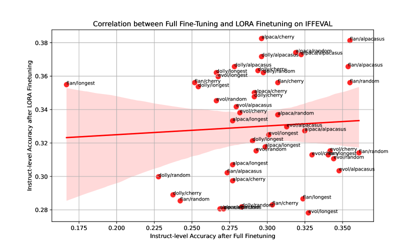
Figure 7: There isn’t any observable correlation between the performance of models finetuned with and without LORA across our setups indicating that we cannot reliably predict the optimal selection strategy on a faster, cost-effective parameter efficient setup.

While it is not possible to largely modify the cost of a selection strategy, it might be possible to offset the cost of finetuning the models on subsets generated via different selection strategies through parameter efficient techniques. If such trends are correlated with the performance of the selected data on the full variant of the model, NLP practioners can potentially design a set of relatively low-cost experiments to rapidly identify the optimal selection strategy to further carry out their selection. Recent work like Xia et al. (2024), even leverage such correlation to achieve great efficiency in task-specific instruction selection. For preliminary experimentation, we rerun all our experiments with the modification of including LORA modules in our finetuning. This reduces the memory footprint of training by to only 0.0038 times of the memory footprint of full finetuning along with faster training by half of its full-finetuning counterpart. In 7 we plot the correlation between the instruct-level-accuracy on IFEVAL for models trained with and without LORA. However, we don’t find any reasonable correlation between these performances highlighlting a need to identify cost-effective methods of predicting the suitability of a custom budget and source distribution to a given selection strategy.

B.2 Benchmark Evaluations for All Configurations

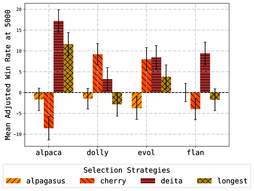
Figure 8: AlpacaEval Length Controlled Win Rate at 5K: Models do not show a consistent trend in performance when scaled from 1000 samples or across datasets.

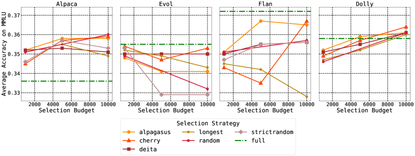
(a) $M_{\text{random}}$versus $M_{\text{selected}}$on MMLU

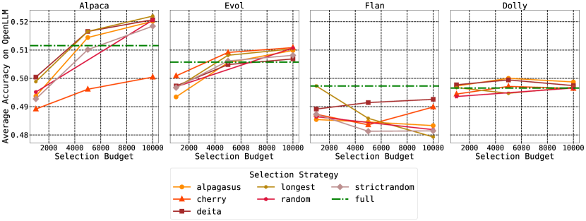
(b) $M_{\text{random}}$versus $M_{\text{selected}}$on OPENLLM

Figure 9: Comparison of $M_{\text{random}}$and $M_{\text{selected}}$on different models

B.3 Correlation between all Benchmarks

B.4 Cost Versus Performance Trade-Offs for All Budgets

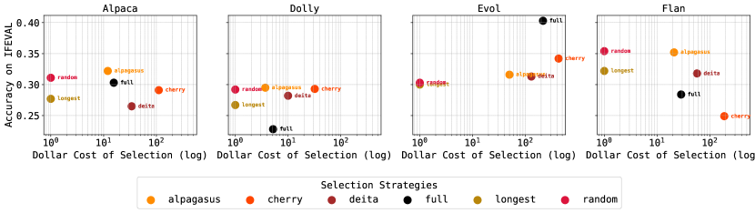
Figure 12: Cost Versus Performance Comparison at 5K budget: We highlight that random performs competitively across most setups

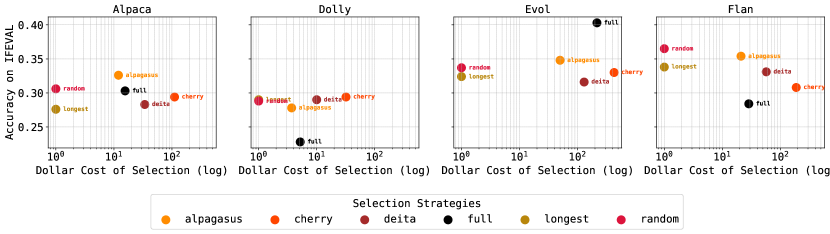
Figure 13: Cost Versus Performance Comparison at 10K:We highlight that random performs competitively across most setups

References

- Cao et al. (2023) Yihan Cao, Yanbin Kang, Chi Wang, and Lichao Sun. 2023. Instruction mining: When data mining meets large language model finetuning.
- Chen et al. (2023) Lichang Chen, Shiyang Li, Jun Yan, Hai Wang, Kalpa Gunaratna, Vikas Yadav, Zheng Tang, Vijay Srinivasan, Tianyi Zhou, Heng Huang, et al. 2023. Alpagasus: Training a better alpaca with fewer data. arXiv preprint arXiv:2307.08701.
- Conover et al. (2023) Mike Conover, Matt Hayes, Ankit Mathur, Jianwei Xie, Jun Wan, Sam Shah, Ali Ghodsi, Patrick Wendell, Matei Zaharia, and Reynold Xin. 2023. Free dolly: Introducing the world’s first truly open instruction-tuned llm.
- Du et al. (2023) Qianlong Du, Chengqing Zong, and Jiajun Zhang. 2023. Mods: Model-oriented data selection for instruction tuning. ArXiv, abs/2311.15653.
- Gao et al. (2023) Leo Gao, Jonathan Tow, Baber Abbasi, Stella Biderman, Sid Black, Anthony DiPofi, Charles Foster, Laurence Golding, Jeffrey Hsu, Alain Le Noac’h, Haonan Li, Kyle McDonell, Niklas Muennighoff, Chris Ociepa, Jason Phang, Laria Reynolds, Hailey Schoelkopf, Aviya Skowron, Lintang Sutawika, Eric Tang, Anish Thite, Ben Wang, Kevin Wang, and Andy Zou. 2023. A framework for few-shot language model evaluation.
- Ge et al. (2024) Yuan Ge, Yilun Liu, Chi Hu, Weibin Meng, Shimin Tao, Xiaofeng Zhao, Hongxia Ma, Li Zhang, Hao Yang, and Tong Xiao. 2024. Clustering and ranking: Diversity-preserved instruction selection through expert-aligned quality estimation. Preprint, arXiv:2402.18191.
- Gema et al. (2024) Aryo Pradipta Gema, Joshua Ong Jun Leang, Giwon Hong, Alessio Devoto, Alberto Carlo Maria Mancino, Rohit Saxena, Xuanli He, Yu Zhao, Xiaotang Du, Mohammad Reza Ghasemi Madani, Claire Barale, Robert McHardy, Joshua Harris, Jean Kaddour, Emile van Krieken, and Pasquale Minervini. 2024. Are we done with mmlu? ArXiv, abs/2406.04127.
- Hu et al. (2021) J. Edward Hu, Yelong Shen, Phillip Wallis, Zeyuan Allen-Zhu, Yuanzhi Li, Shean Wang, and Weizhu Chen. 2021. Lora: Low-rank adaptation of large language models. ArXiv, abs/2106.09685.
- Li et al. (2024) Ming Li, Yong Zhang, Shwai He, Zhitao Li, Hongyu Zhao, Jianzong Wang, Ning Cheng, and Tianyi Zhou. 2024. Superfiltering: Weak-to-strong data filtering for fast instruction-tuning. Preprint, arXiv:2402.00530.
- Li et al. (2023a) Ming Li, Yong Zhang, Zhitao Li, Jiuhai Chen, Lichang Chen, Ning Cheng, Jianzong Wang, Tianyi Zhou, and Jing Xiao. 2023a. From quantity to quality: Boosting llm performance with self-guided data selection for instruction tuning. ArXiv, abs/2308.12032.
- Li et al. (2023b) Xuechen Li, Tianyi Zhang, Yann Dubois, Rohan Taori, Ishaan Gulrajani, Carlos Guestrin, Percy Liang, and Tatsunori B. Hashimoto. 2023b. Alpacaeval: An automatic evaluator of instruction-following models. https://github.com/tatsu-lab/alpaca_eval.
- Liu et al. (2023) Wei Liu, Weihao Zeng, Keqing He, Yong Jiang, and Junxian He. 2023. What makes good data for alignment? a comprehensive study of automatic data selection in instruction tuning. ArXiv, abs/2312.15685.
- Liu et al. (2024) Ziche Liu, Rui Ke, Feng Jiang, and Haizhou Li. 2024. Take the essence and discard the dross: A rethinking on data selection for fine-tuning large language models. ArXiv, abs/2406.14115.
- Longpre et al. (2023) S. Longpre, Le Hou, Tu Vu, Albert Webson, Hyung Won Chung, Yi Tay, Denny Zhou, Quoc V. Le, Barret Zoph, Jason Wei, and Adam Roberts. 2023. The flan collection: Designing data and methods for effective instruction tuning. In International Conference on Machine Learning.
- Lou et al. (2024) Renze Lou, Kai Zhang, and Wenpeng Yin. 2024. Large language model instruction following: A survey of progresses and challenges. Preprint, arXiv:2303.10475.
- Lu et al. (2023) Yao Lu, Jiayi Wang, Sebastian Riedel, and Pontus Stenetorp. 2023. Strings from the library of babel: Random sampling as a strong baseline for prompt optimisation. In North American Chapter of the Association for Computational Linguistics.
- Mekala et al. (2024) Dheeraj Mekala, Alex Nguyen, and Jingbo Shang. 2024. Smaller language models are capable of selecting instruction-tuning training data for larger language models. In Findings of the Association for Computational Linguistics ACL 2024, pages 10456–10470, Bangkok, Thailand and virtual meeting. Association for Computational Linguistics.
- Pan et al. (2024) Xingyuan Pan, Luyang Huang, Liyan Kang, Zhicheng Liu, Yu Lu, and Shanbo Cheng. 2024. G-DIG: Towards gradient-based DIverse and hiGh-quality instruction data selection for machine translation. In Proceedings of the 62nd Annual Meeting of the Association for Computational Linguistics (Volume 1: Long Papers), pages 15395–15406, Bangkok, Thailand. Association for Computational Linguistics.
- Panickssery et al. (2024) Arjun Panickssery, Samuel R. Bowman, and Shi Feng. 2024. Llm evaluators recognize and favor their own generations. Preprint, arXiv:2404.13076.
- Qin et al. (2024a) Yiwei Qin, Kaiqiang Song, Yebowen Hu, Wenlin Yao, Sangwoo Cho, Xiaoyang Wang, Xuansheng Wu, Fei Liu, Pengfei Liu, and Dong Yu. 2024a. Infobench: Evaluating instruction following ability in large language models. Preprint, arXiv:2401.03601.
- Qin et al. (2024b) Yulei Qin, Yuncheng Yang, Pengcheng Guo, Gang Li, Hang Shao, Yuchen Shi, Zihan Xu, Yun Gu, Ke Li, and Xing Sun. 2024b. Unleashing the power of data tsunami: A comprehensive survey on data assessment and selection for instruction tuning of language models. Preprint, arXiv:2408.02085.
- Shen (2024) Ming Shen. 2024. Rethinking data selection for supervised fine-tuning. Preprint, arXiv:2402.06094.
- Shen et al. (2023) Tianhao Shen, Renren Jin, Yufei Huang, Chuang Liu, Weilong Dong, Zishan Guo, Xinwei Wu, Yan Liu, and Deyi Xiong. 2023. Large language model alignment: A survey. ArXiv, abs/2309.15025.
- Taori et al. (2023) Rohan Taori, Ishaan Gulrajani, Tianyi Zhang, Yann Dubois, Xuechen Li, Carlos Guestrin, Percy Liang, and Tatsunori B. Hashimoto. 2023. Stanford alpaca: An instruction-following llama model. https://github.com/tatsu-lab/stanford_alpaca.
- Touvron et al. (2023) Hugo Touvron, Thibaut Lavril, Gautier Izacard, Xavier Martinet, Marie-Anne Lachaux, Timothée Lacroix, Baptiste Rozière, Naman Goyal, Eric Hambro, Faisal Azhar, Aurelien Rodriguez, Armand Joulin, Edouard Grave, and Guillaume Lample. 2023. Llama: Open and efficient foundation language models. ArXiv, abs/2302.13971.
- van der Meer et al. (2024) Michiel van der Meer, Neele Falk, Pradeep K. Murukannaiah, and Enrico Liscio. 2024. Annotator-centric active learning for subjective nlp tasks. Preprint, arXiv:2404.15720.
- Wang et al. (2024) Jiahao Wang, Bolin Zhang, Qianlong Du, Jiajun Zhang, and Dianhui Chu. 2024. A survey on data selection for llm instruction tuning. Preprint, arXiv:2402.05123.
- Wei et al. (2023) Lai Wei, Zihao Jiang, Weiran Huang, and Lichao Sun. 2023. Instructiongpt-4: A 200-instruction paradigm for fine-tuning minigpt-4. Preprint, arXiv:2308.12067.
- Xia et al. (2024) Mengzhou Xia, Sadhika Malladi, Suchin Gururangan, Sanjeev Arora, and Danqi Chen. 2024. Less: Selecting influential data for targeted instruction tuning. ArXiv, abs/2402.04333.
- Xie et al. (2023a) Sang Michael Xie, Shibani Santurkar, Tengyu Ma, and Percy Liang. 2023a. Data selection for language models via importance resampling. In Thirty-seventh Conference on Neural Information Processing Systems.
- Xie et al. (2023b) Sang Michael Xie, Shibani Santurkar, Tengyu Ma, and Percy Liang. 2023b. Data selection for language models via importance resampling. ArXiv, abs/2302.03169.
- Xu et al. (2023) Can Xu, Qingfeng Sun, Kai Zheng, Xiubo Geng, Pu Zhao, Jiazhan Feng, Chongyang Tao, and Daxin Jiang. 2023. Wizardlm: Empowering large language models to follow complex instructions. ArXiv, abs/2304.12244.
- Yauney and Mimno (2024) Gregory Yauney and David M. Mimno. 2024. Stronger random baselines for in-context learning. ArXiv, abs/2404.13020.
- Zeng et al. (2023) Zhiyuan Zeng, Jiatong Yu, Tianyu Gao, Yu Meng, Tanya Goyal, and Danqi Chen. 2023. Evaluating large language models at evaluating instruction following. ArXiv, abs/2310.07641.
- Zhao et al. (2024) Hao Zhao, Maksym Andriushchenko, Francesco Croce, and Nicolas Flammarion. 2024. Long is more for alignment: A simple but tough-to-beat baseline for instruction fine-tuning.
- Zheng et al. (2024) Xiaosen Zheng, Tianyu Pang, Chao Du, Qian Liu, Jing Jiang, and Min Lin. 2024. Cheating automatic llm benchmarks: Null models achieve high win rates.
- Zhou et al. (2023a) Chunting Zhou, Pengfei Liu, Puxin Xu, Srini Iyer, Jiao Sun, Yuning Mao, Xuezhe Ma, Avia Efrat, Ping Yu, L. Yu, Susan Zhang, Gargi Ghosh, Mike Lewis, Luke Zettlemoyer, and Omer Levy. 2023a. Lima: Less is more for alignment. ArXiv, abs/2305.11206.
- Zhou et al. (2023b) Jeffrey Zhou, Tianjian Lu, Swaroop Mishra, Siddhartha Brahma, Sujoy Basu, Yi Luan, Denny Zhou, and Le Hou. 2023b. Instruction-following evaluation for large language models. ArXiv, abs/2311.07911.