Robust Low-rank Tensor Train Recovery

Abstract

Tensor train (TT) decomposition represents an $N$-order tensor using $O(N)$ matrices (i.e., factors) of small dimensions, achieved through products among these factors. Due to its compact representation, TT decomposition has found wide applications, including various tensor recovery problems in signal processing and quantum information. In this paper, we study the problem of reconstructing a TT format tensor from measurements that are contaminated by outliers with arbitrary values. Given the vulnerability of smooth formulations to corruptions, we use an $\ell_{1}$ loss function to enhance robustness against outliers. We first establish the $\ell_{1}/\ell_{2}$-restricted isometry property (RIP) for Gaussian measurement operators, demonstrating that the information in the TT format tensor can be preserved using a number of measurements that grows linearly with $N$. We also prove the sharpness property for the $\ell_{1}$ loss function optimized over TT format tensors. Building on the $\ell_{1}/\ell_{2}$-RIP and sharpness property, we then propose two complementary methods to recover the TT format tensor from the corrupted measurements: the projected subgradient method (PSubGM), which optimizes over the entire tensor, and the factorized Riemannian subgradient method (FRSubGM), which optimizes directly over the factors. Compared to PSubGM, the factorized approach FRSubGM significantly reduces the memory cost at the expense of a slightly slower convergence rate. Nevertheless, we show that both methods, with diminishing step sizes, converge linearly to the ground-truth tensor given an appropriate initialization, which can be obtained by a truncated spectral method. To the best of our knowledge, this is the first work to provide a theoretical analysis of the robust TT recovery problem and to demonstrate that TT-format tensors can be robustly recovered even when up to half of the measurements are arbitrarily corrupted. We conduct various numerical experiments to demonstrate the effectiveness of the two methods in robust TT recovery.

Keywords: Tensor-train decomposition, Robust tensor recovery, $\ell_{1}/\ell_{2}$-RIP, Sharpness, Projected subgradient method, factorized Riemannian subgradient method, linear convergence.

1 Introduction

Tensor recovery has been widely investigated in many areas, such as signal processing and machine learning [1, 2], communication [3], quantum physics [4, 5, 6], chemometrics [7, 8], genetic engineering [9], and so on. One fundamental task is to recover a tensor $\mathcal{X}^{\star}\in\mathbb{R}^{d_{1}\times\cdots\times d_{N}}$ from highly incomplete, sometimes even corrupted, observations $\bm{y}=\{y_{k}\}_{k=1}^{m}$ given by

$$\bm{y}=\mathcal{A}(\mathcal{X}^{\star})+\bm{s}=\begin{bmatrix}y_{1}\\ \vdots\\ y_{m}\end{bmatrix}=\begin{bmatrix}\langle\mathcal{A}_{1},\mathcal{X}^{\star}\rangle+s_{1}\\ \vdots\\ \langle\mathcal{A}_{m},\mathcal{X}^{\star}\rangle+s_{m}\end{bmatrix}\in\mathbb{R}^{m},$$ (1)

where $\mathcal{A}(\mathcal{X}^{\star}):\mathbb{R}^{d_{1}\times\cdots\times d_{N}}\rightarrow\mathbb{R}^{m}$ is a linear observation operator that models the measurement process and $\bm{s}\in\mathbb{R}^{m}$ represents an outlier vector, wherein only a small fraction of its entries (referred to as outliers) have arbitrary magnitudes but their locations are unknown a prior, while the remaining entries are zero. In practical scenarios, outliers are frequently encountered in sensing or regression models [10, 11, 12, 13, 14, 15, 16, 17, 5, 6], stemming from various factors such as sensor malfunctions and malicious attacks. For instance, in quantum state tomography, imperfections during quantum state preparation can randomly generate unwarranted outlier quantum states, which subsequently lead to outliers during the measurement operation [18, 19, 14].

Even in the absence of outliers, the recovery from (1) remains ill-posed due to the curse of dimensionality, which arises from the exponential storage complexity of $\mathcal{X}^{\star}$ with respect to $N$. Therefore, it is often advantageous (and even necessary) to employ certain tensor decomposition models to compactly represent the full tensor. One commonly used model is the tensor train (TT) decomposition [20], which expresses the $(s_{1},\dots,s_{N})$-th element of $\mathcal{X}^{\star}$ as the following matrix product form [20]

$$\mathcal{X}^{\star}(s_{1},\dots,s_{N})=\bm{X}_{1}^{\star}(:,s_{1},:)\bm{X}_{2}^{\star}(:,s_{2},:)\cdots\bm{X}_{N}^{\star}(:,s_{N},:),$$ (2)

where tensor factors ${\bm{X}}_{i}^{\star}\in\mathbb{R}^{r_{i-1}\times d_{i}\times r_{i}},i\in[N]$ with $r_{0}=r_{N}=1$. The dimensions $\text{rank}(\mathcal{X}^{\star})=(r_{1},\dots,r_{N-1})$ of such a decomposition are called the TT ranks of $\mathcal{X}^{\star}$. We say a TT format tensor is low-rank if $r_{i}$ is much smaller compared to $\min\{\Pi_{j=1}^{i}d_{j},\Pi_{j=i+1}^{N}d_{j}\}$ for most indices $i$ so that the total number of parameters in the tensor factors $\{\bm{X}_{i}^{\star}\}$ is much smaller than the number of entries in $\mathcal{X}^{\star}$. We refer to any tensor for which such a low-rank TT decomposition exists as a low-TT-rank tensor. To simplify the notation, we may also use $[\bm{X}_{1}^{\star},\dots,\bm{X}_{N}^{\star}]$ as the compact form of $\mathcal{X}^{\star}$.

Compared to the other two commonly used tensor decompositions—canonical polyadic (CP) [21] and Tucker [22] decompositions—TT decomposition strikes a balance between the advantages of both approaches. The number of parameters of TT decomposition is $O(N\overline{d}\overline{r}^{2})$ with $\overline{d}=\max_{i}d_{i}$ and $\overline{r}=\max_{i}r_{i}$, not growing exponentially with the tensor order as the CP decomposition. Furthermore, similar to the Tucker decomposition, the TT decomposition can be approximately computed using an SVD-based algorithm, called the tensor train SVD (TT-SVD), with a guaranteed accuracy [20]. See [25] for a detailed description. Consequently, TT decomposition has been widely applied to tensor recovery across various fields, including quantum tomography [6], neuroimaging [13], facial model refinement [26], and the distinction of its attributes [27], longitudinal relational data analysis [28], and forecasting tasks [29].

Our goals and main results

In this paper, we study the robust recovery problem in (1), where the underlying tensor $\mathcal{X}^{\star}$ has low TT ranks. We refer to this as the robust TT recovery problem. To handle outliers in the measurements, we employ a robust $\ell_{1}$ loss function together with the TT format and solve the following problem:

$$\begin{split}\min_{\mbox{\tiny$\begin{array}[]{c}\mathcal{X}\in\mathbb{R}^{d_{1}\times\cdots\times d_{N}}\\ \text{rank}(\mathcal{X})=(r_{1},\dots,r_{N-1})\end{array}$}}f(\mathcal{X})=\frac{1}{m}\|\mathcal{A}(\mathcal{X})-\bm{y}\|_{1}.\end{split}$$ (3)

Compared to the conventional least-squares loss, the $\ell_{1}$ loss function is more robust against outliers and has been widely adopted in robust signal recovery problems [30, 14, 31, 32, 33, 34, 35, 36, 37, 17]. However, the combination of the $\ell_{1}$ loss function and TT decomposition makes the problem (3) highly nonsmooth and nonconvex. Our goal is to study its optimality conditions and develop optimization algorithms with guaranteed performance.

Note that measurements should satisfy certain properties to enable robust recovery from corrupted measurements. Thus, we first study the stable embedding of low-TT-rank tensors by establishing the following $\ell_{1}/\ell_{2}$-restricted isometry property ($\ell_{1}/\ell_{2}$-RIP) without outliers for $\mathcal{A}$, which has been introduced previously in the context of low-rank matrix/Tucker tensor recovery [39, 40, 34, 17, 41] and covariance estimation [42]. This mixed-norm approximate isometry evaluates the signal strength before and after projection using different metrics: the input is measured in terms of the Frobenius norm, and the output is measured in terms of the $\ell_{1}$ norm. Specifically, we say $\mathcal{A}$ satisfies rank-$\overline{r}$ $\ell_{1}/\ell_{2}$-RIP if there exits a constant $\delta_{\overline{r}}\in(0,\sqrt{2/\pi})$ such that

$$(\sqrt{2/\pi}-\delta_{\overline{r}})\|\mathcal{X}\|_{F}\leq\frac{1}{m}\|\mathcal{A}(\mathcal{X})\|_{1}\leq(\sqrt{2/\pi}+\delta_{\overline{r}})\|\mathcal{X}\|_{F}$$ (4)

holds for all low-TT-rank tensors with ranks $(r_{1},\dots,r_{N-1}),r_{i}\leq\overline{r}$. We show that Gaussian measurement operators $\mathcal{A}$, where $\mathcal{A}_{1},\dots,\mathcal{A}_{m}$ have independent and identically distributed (i.i.d.) standard Gaussian entries, satisfies $\ell_{1}/\ell_{2}$-RIP (4) with high probability as long as $m\geq\Omega(N\overline{d}\overline{r}^{2}\log N/\delta_{\overline{r}}^{2})$ with $\overline{d}=\max_{i}d_{i}$. This implies that robust TT recovery is possible using a number of measurements that only scale (approximately) linearly with regard to $N$. With the $\ell_{1}/\ell_{2}$-RIP property, we show that the robust loss function in (3) satisfies the sharpness property [43, 44, 34, 45, 17, 41]: for any low-TT-rank tensors $\mathcal{X}$ with TT ranks $r_{i}\leq\overline{r}$, it holds that

$$\frac{1}{m}\|\mathcal{A}(\mathcal{X}-\mathcal{X}^{\star})-\bm{s}\|_{1}-\frac{1}{m}\|\bm{s}\|_{1}\geq((1-2p_{s})\sqrt{2/\pi}-\delta_{\overline{r}})\|\mathcal{X}-\mathcal{X}^{\star}\|_{F},$$ (5)

where $p_{s}\in[0,0.5]$ represents the fraction of outliers in $\bm{y}$, i.e., $p_{s}=\|\bm{s}\|_{0}/m$. Since (3) optimizes only over low-TT-rank tensors, (5) needs to hold only for these tensors; as such, a similar condition for Tucker tensors is also referred to as restricted sharpness in [17, 41]. The sharpness condition (5) implies that $\mathcal{X}^{\star}$ is the unique global minimum, with the loss function increasing as the variable $\mathcal{X}$ deviates from $\mathcal{X}^{\star}$.

Our second contribution is to propose two complementary iterative algorithms for solving (3). Building on insights from [38], we introduce a projected subgradient method (PSubGM). This method optimizes the entire tensor in each iteration and employs the TT-SVD to project the iterates back to the TT format. Under the sharpness property, we establish a robust regularity condition (RRC) for the objective function (3). We show that the PSubGM algorithm, with appropriate initialization and diminishing step sizes, achieves a linear convergence rate. Remarkably, PSubGM can precisely recover the ground-truth tensor $\mathcal{X}^{\star}$ even in the presence of outliers.

A potential drawback of PSubGM when handling high-order tensors is that it requires storing the full estimated tensor $\mathcal{X}$ and performing TT-SVD at each iteration, which becomes impractical for large $N$, such as in quantum state tomography involving hundreds of qubits [6]. To address this issue, instead of optimizing directly over the tensor $\mathcal{X}$, we employ the factorization approach that optimizes over the factors $\{\bm{X}_{i}\}_{i\geq 1}$ which can significantly reduce the memory cost. Specifically, we consider the following optimization problem:

$$\begin{split}\min_{\mbox{\tiny$\begin{array}[]{c}\bm{X}_{i}\in\mathbb{R}^{r_{i-1}\times d_{i}\times r_{i}},\\ i\in[N]\end{array}$}}&\frac{1}{m}\|\mathcal{A}([\bm{X}_{1},\dots,\bm{X}_{N}])-\bm{y}\|_{1},\\ &\operatorname*{s.t.\ }\ \sum_{s_{i}=1}^{d_{i}}\bm{X}_{i}^{\top}(:,s_{i},:)\bm{X}_{i}(:,s_{i},:)={\bf I}_{r_{i}},\ \ i\in[N-1].\end{split}$$ (6)

The additional constraints $\sum_{s_{i}=1}^{d_{i}}\bm{X}_{i}^{\top}(:,s_{i},:)\bm{X}_{i}(:,s_{i},:)={\bf I}_{r_{i}}$ are introduced to reduce the scaling ambiguity of the factors [46]. The orthogonality constraints can be viewed as Stiefel manifolds of Riemannian space, so we utilize a factorized Riemannian subgradient method (FRSubGM) on the Stiefel manifold to optimize (6). We show that the objective function (6) also satisfies a Riemannian RRC, and prove that the FRSubGM algorithm, with an appropriate initialization and a diminishing step size, converges to the ground-truth tensor $\mathcal{X}^{\star}$ at a linear rate. Finally, we present a guaranteed truncated spectral initialization as a valid starting point, ensuring linear convergence for both the PSubGM and FRSubGM algorithms.

In Table 1, we summarize the convergence results for PSubGM and FRSubGM and compare them with previous results on tensor recovery in the absence of outliers, specifically the IHT [38, 47] and factorized Riemannian gradient descent (FRGD) [46] that solve problems similar to (3) and the factorized problem (6), with the objective function being changed to a smooth $\ell_{2}$ loss function. We observe that PSubGM and FRSubGM achieve a similar linear convergence rate as their smooth counterparts, demonstrating that the outliers can be handled as easily as in the noiseless case by the nonconvex optimization approaches. The convergence rate of IHT/PSubGM primarily hinges on the RIP constant, with a potential decay ($1+c$) (where $c$ is a universal constant) owing to the expansiveness of the TT-SVD. Conversely, the convergence rate of FRGD/FRSubGM relies not only on the RIP constant but also on factors like $N$, $\overline{r}$, and $\mathcal{X}^{\star}$, which could impede the convergence speed.

Table 1: Comparison of IHT/FRGD for solving TT recovery with noiseless measurements and PSubGM/FRSubGM for the corrupted measurements. Here $p_{s}$ denotes the fraction of outliers in the measurements. The upper bound of initialization is expressed in terms of $\|\mathcal{X}^{(0)}-\mathcal{X}^{\star}\|_{F}$. The convergence rates of IHT, PSubGM and FRGD, FRSubGM are respectively analyzed concerning $\|\mathcal{X}^{(t)}-\mathcal{X}^{\star}\|_{F}^{2}$ and $\text{dist}^{2}(\{\bm{X}_{i}^{(t)}\},\{\bm{X}_{i}^{\star}\})$ defined in (24). $\delta_{\overline{r}}^{\prime}\in(0,1)$ is a constant in standard $\ell_{2}/\ell_{2}$-RIP (see [6, Theorem 2]), while $\delta_{\overline{r}}\in(0,1)$ is a constant in $\ell_{1}/\ell_{2}$-RIP. $c$ is a universal constant.

Algorithm	Outlier	Initialization Requirement	Rate of Convergence	RIP condition
IHT [38, 47]	$\times$	$\frac{c\underline{\sigma}({\mathcal{X}^{\star}})}{600N}$	$(1+c)\big{(}1-\frac{(1-\delta_{4\overline{r}}^{\prime})^{2}}{2(1+\delta_{4\overline{r}}^{\prime})^{2}}\big{)}<1$	$\delta_{4\overline{r}}^{\prime}\leq\frac{1-\sqrt{2c/(1+c)}}{1+\sqrt{2c/(1+c)}}$
FRGD [46]	$\times$	$O\big{(}\frac{\underline{\sigma}^{2}(\mathcal{X}^{\star})}{\overline{r}N^{2}\overline{\sigma}(\mathcal{X}^{\star})}\big{)}$	$1-O\big{(}\frac{(4-15\delta_{(N+3)\overline{r}}^{\prime})^{2}}{(1+\delta_{(N+3)\overline{r}}^{\prime})^{2}N^{2}\overline{r}\kappa^{2}(\mathcal{X}^{\star})}\big{)}$	$\delta_{(N+3)\overline{r}}^{\prime}\leq\frac{4}{15}$
PSubGM	$\surd$	$\frac{c\underline{\sigma}({\mathcal{X}^{\star}})}{600N}$	$(1+c)\big{(}1-\frac{3((1-2p_{s})\sqrt{2/\pi}-\delta_{2\overline{r}})^{2}}{4(\sqrt{2/\pi}+\delta_{2\overline{r}})^{2}}\big{)}<1$	$\delta_{2\overline{r}}<\frac{1-2p_{s}-\sqrt{4c/(3+3c)}}{1+\sqrt{4c/(3+3c)}}\sqrt{\frac{2}{\pi}}$
FRSubGM	$\surd$	$O\big{(}\frac{\underline{\sigma}^{2}(\mathcal{X}^{\star})}{\overline{r}N^{2}\overline{\sigma}(\mathcal{X}^{\star})}\big{)}$	$1-O\big{(}\frac{((1-2p_{s})\sqrt{2/\pi}-\delta_{(N+1)\overline{r}})^{2}}{N^{2}\overline{r}(\sqrt{2/\pi}+\delta_{(N+1)\overline{r}})^{2}\kappa^{2}(\mathcal{X}^{\star})}\big{)}$	$\delta_{(N+1)\overline{r}}\leq(1-2p_{s})\sqrt{\frac{2}{\pi}}$

Related works

Theoretical analyses and algorithmic designs for robust low-rank matrix recovery via nonsmooth optimization have been extensively studied in [48, 34, 37, 45, 49]. A notable advantage of nonsmooth formulations is the enhanced robustness to adversarial outliers, achieved through a simple algorithmic design–the low-rank factors are updated in essentially the same manner, irrespective of the presence of outliers. However, existing theoretical frameworks for asymmetric matrix factorization cannot be extended to robust high-order tensor recovery, as the additional regularization terms introduced to balance the factors may not generalize to multiple tensor factors.

For tensor recovery from a limited number of measurements, most existing theoretical work and algorithmic designs have predominantly focused on developing optimization algorithms for either the noiseless case or the presence of Gaussian noise. Typically, a smooth loss function, such as the residual sum of squares ($\ell_{2}$ loss), is employed. Variants of projected gradient descent (PGD) algorithms, including iterative hard thresholding (IHT) [38, 50, 51] and Riemannian gradient descent on the fixed-rank manifold [52, 53], have been studied for operating on the entire tensor with guaranteed convergence and performance. However, direct optimization over the tensor $\mathcal{X}$ poses a challenge due to its exponentially large memory requirements in terms of $N$. To address this storage issue, factorization approaches [54, 55, 46] have been developed to optimize the factors of a tensor decomposition.

In contrast, tensor recovery from measurements corrupted by outliers has been less studied. Recently, the work [17] introduced the first provably scalable gradient descent algorithm for order-$3$ Tucker recovery from corrupted measurements. To the best of our knowledge, there is a lack of analysis and algorithmic design with guaranteed convergence for robust TT recovery.

Notation: We use calligraphic letters (e.g., $\mathcal{Y}$) to denote tensors, bold capital letters (e.g., $\bm{Y}$) to denote matrices, except for $\bm{X}_{i}$ which denotes the $i$-th order-$3$ tensor factors in the TT format, bold lowercase letters (e.g., $\bm{y}$) to denote vectors, and italic letters (e.g., $y$) to denote scalar quantities. Elements of matrices and tensors are denoted in parentheses, as in Matlab notation. For example, $\mathcal{X}(i_{1},i_{2},i_{3})$ denotes the element in position $(i_{1},i_{2},i_{3})$ of the order-3 tensor $\mathcal{X}$. The inner product of $\mathcal{A}\in\mathbb{R}^{d_{1}\times\dots\times d_{N}}$ and $\mathcal{B}\in\mathbb{R}^{d_{1}\times\dots\times d_{N}}$ can be denoted as $\langle\mathcal{A},\mathcal{B}\rangle=\sum_{s_{1}=1}^{d_{1}}\cdots\sum_{s_{N}=1}^{d_{N}}\mathcal{A}(s_{1},\dots,s_{N})\mathcal{B}(s_{1},\dots,s_{N})$. The vectorization of $\mathcal{X}\in\mathbb{R}^{d_{1}\times\dots\times d_{N}}$, denoted as $\text{vec}(\mathcal{X})$, transforms the tensor $\mathcal{X}$ into a vector. The $(s_{1},\dots,s_{N})$-th element of $\mathcal{X}$ can be found in the vector $\text{vec}(\mathcal{X})$ at the position $s_{1}+d_{1}(s_{2}-1)+\cdots+d_{1}d_{2}\cdots d_{N-1}(s_{N}-1)$. $\|\mathcal{X}\|_{F}=\sqrt{\langle\mathcal{X},\mathcal{X}\rangle}$ is the Frobenius norm of $\mathcal{X}$. $\|\bm{X}\|$ and $\|\bm{X}\|_{F}$ respectively represent the spectral norm and Frobenius norm of $\bm{X}$. $\sigma_{i}(\bm{X})$ is the $i$-th singular value of $\bm{X}$. $\|\bm{x}\|_{2}$ denotes the $\ell_{2}$ norm of $\bm{x}$. For a positive integer $K$, $[K]$ denotes the set $\{1,\dots,K\}$. For two positive quantities $a,b\in\mathbb{R}$, $b=O(a)$ means $b\leq ca$ for some universal constant $c$; likewise, $b=\Omega(a)$ represents $b\geq ca$ for some universal constant $c$. To simplify notations in the following sections, for an order-$N$ TT format tensor with ranks $(r_{1},\dots,r_{N-1})$, we define $\overline{r}=\max_{i=1}^{N-1}r_{i}$ and $\overline{d}=\max_{i=1}^{N}d_{i}$.

2 $\ell_{1}/\ell_{2}$-Restricted Isometry Property and Sharpness for Robust TT Recovery

2.1 Tensor train decomposition

Recall the TT format in (2). Considering that $\bm{X}_{i}(:,s_{i},:)$ will be extensively used, we denote it by $\bm{X}_{i}(s_{i})\in\mathbb{R}^{r_{i-1}\times r_{i}}$ as one “slice” of $\bm{X}_{i}$ with the second index being fixed at $s_{i}$. Thus, for any $\mathcal{X}=[\bm{X}_{1},\dots,\bm{X}_{N}]\in\mathbb{R}^{d_{1}\times\dots\times d_{N}}$ in the TT format, we can express its $(s_{1},\dots,s_{N})$-th element as the following matrix product form

$$\mathcal{X}(s_{1},\dots,s_{N})=\prod_{i=1}^{N}\bm{X}_{i}(:,s_{i},:)=\prod_{i=1}^{N}\bm{X}_{i}(s_{i}).$$ (7)

We may also arrange the slices $\{\bm{X}_{i}(s_{i})\}_{s_{i}=1}^{d_{i}}$ into the following form:

$$L(\bm{X}_{i})=\begin{bmatrix}\bm{X}_{i}(1)\\ \vdots\\ \bm{X}_{i}(d_{i})\end{bmatrix}\in\mathbb{R}^{d_{i}r_{i-1}\times r_{i}},\ \ \forall i\in[N],$$ (8)

where $L(\bm{X}_{i})$ is often referred to as the left unfolding of $\bm{X}_{i}$ when viewing $\bm{X}_{i}$ as a tensor.

The decomposition of the tensor $\mathcal{X}$ into the form of (7) is generally not unique: not only the factors $\bm{X}_{i}(s_{i})$ are not unique, but also the dimension of these factors can vary. According to [56], there exists a unique set of ranks $\bm{r}=(r_{1},\dots,r_{N-1})$ for which $\mathcal{X}$ admits a minimal TT decomposition. We say the decomposition (7) is minimal if the rank of the left unfolding matrix $L(\bm{X}_{i})$ in (8) is $r_{i}$. In addition, the factors can be chosen such that $L(\bm{X}_{i})$ is orthonormal for all $i\in[N-1]$; that is

$$L^{\top}(\bm{X}_{i})L(\bm{X}_{i})={\bf I}_{r_{i}},\ \ i\in[N-1].$$ (9)

The resulting TT decomposition is called the left-orthogonal format of $\mathcal{X}$. Moreover, in this case, $r_{i}$ equals to the rank of the $i$-th unfolding matrix $\mathcal{X}^{\langle i\rangle}\in\mathbb{R}^{(d_{1}\cdots d_{k})\times(d_{k+1}\cdots d_{N})}$ of the tensor $\mathcal{X}$, where the $(s_{1}\cdots s_{i},s_{i+1}\cdots s_{N})$-th element of $\mathcal{X}^{\langle i\rangle}$ is given by $\mathcal{X}^{\langle i\rangle}(s_{1}\cdots s_{i},s_{i+1}\cdots s_{N})=\mathcal{X}(s_{1},\dots,s_{N})$. This can also serve as an alternative way to define the TT rank. With the $i$-th unfolding matrix $\mathcal{X}^{\langle i\rangle}$ and TT ranks, we can define its smallest singular value $\underline{\sigma}(\mathcal{X})=\min_{i=1}^{N-1}\sigma_{r_{i}}(\mathcal{X}^{\langle i\rangle})$, its largest singular value $\overline{\sigma}(\mathcal{X})=\max_{i=1}^{N-1}\sigma_{1}(\mathcal{X}^{\langle i\rangle})$ and condition number $\kappa(\mathcal{X})=\frac{\overline{\sigma}(\mathcal{X})}{\underline{\sigma}(\mathcal{X})}$.

2.2 $\ell_{1}/\ell_{2}$-Restricted Isometry Property

We first prove the $\ell_{1}/\ell_{2}$-RIP property for the robust TT recovery problem with Gaussian measurement operators, a “gold standard” for studying random linear measurements in the compressive sensing literature [57, 58, 59, 60, 61]. As previously studied in the contexts of low-rank matrix and Tucker tensor recovery problems [39, 40, 34, 17] and covariance estimation [42], $\ell_{1}/\ell_{2}$-RIP establishes a connection between $\|\mathcal{A}(\mathcal{X})\|_{1}$ and $\|\mathcal{X}\|_{F}$, differing from previous work on $\ell_{2}/\ell_{2}$-RIP [38, 6] on TT recovery problem, which examine the relationship between $\|\mathcal{A}(\mathcal{X})\|_{2}^{2}$ and $\|\mathcal{X}\|_{F}^{2}$.

Theorem 1.

($\ell_{1}/\ell_{2}$-RIP of Gaussian measurement operators) Suppose the linear map $\mathcal{A}:\mathbb{R}^{d_{1}\times\cdots\times d_{N}}\rightarrow\mathbb{R}^{m}$ is a Gaussian measurement operator where $\{\mathcal{A}_{k}\}_{k=1}^{m}$ have i.i.d. standard Gaussian entries. Let $\delta_{\overline{r}}\in(0,\sqrt{2/\pi})$ be a positive constant. If the number of measurements satisfies $m\geq\Omega(N\overline{d}\overline{r}^{2}\log N/\delta_{\overline{r}}^{2})$, then with probability exceeding $1-e^{-\Omega(N\overline{d}\overline{r}^{2}\log N)}$, $\mathcal{A}$ satisfies the $\ell_{1}/\ell_{2}$-restricted isometry property in the sense that

$$(\sqrt{2/\pi}-\delta_{\overline{r}})\|\mathcal{X}\|_{F}\leq\frac{1}{m}\|\mathcal{A}(\mathcal{X})\|_{1}\leq(\sqrt{2/\pi}+\delta_{\overline{r}})\|\mathcal{X}\|_{F}$$ (10)

hold for all low-TT-rank tensors $\mathcal{X}$ with ranks $\bm{r}=(r_{1},\dots,r_{N-1})$.

The proof is provided in Appendix B. Theorem 1 guarantees the RIP for Gaussian measurements where the number of measurements $m$ scales linearly, rather than exponentially, with respect to the tensor order $N$. When RIP holds, then for any two distinct TT format tensors $\mathcal{X}_{1},\mathcal{X}_{2}$ with TT ranks smaller than $\overline{r}$, we have distinct measurements since

$$\frac{1}{m}\|\mathcal{A}(\mathcal{X}_{1})-\mathcal{A}(\mathcal{X}_{2})\|_{1}=\frac{1}{m}\|\mathcal{A}(\mathcal{X}_{1}-\mathcal{X}_{2})\|_{1}\geq(\sqrt{2/\pi}-\delta_{2\overline{r}})\|\mathcal{X}_{1}-\mathcal{X}_{2}\|_{F},$$ (11)

which guarantees the possibility of exact recovery in the absence of outliers. In addition, we note that Theorem 1 can also be applicable to other measurement operators, such as subgaussian measurements [62], using a similar analysis.

2.3 Sharpness

We now study the $\ell_{1}$ loss function $f(\mathcal{X})=\frac{1}{m}\|\mathcal{A}(\mathcal{X})-\bm{y}\|_{1}$ and establish the sharpness property [43, 44] that can ensure exact recovery with corrupted measurements in (1). Let $\mathcal{S}\subseteq\{1,\dots,m\}$ denote the support of the outlier vector $\bm{s}$, and $\mathcal{S}^{c}=\{1,\dots,m\}\backslash\mathcal{S}$. We define $p_{s}=\frac{|\mathcal{S}|}{m}$ as the fraction of outliers in $\bm{y}$. The following result establishes the sharpness property for $\mathcal{A}$.

Lemma 1.

(Sharpness of Gaussian measurement operators) Given an unknown target tensor $\mathcal{X}^{\star}$ with ranks $\bm{r}=(r_{1},\dots,r_{N-1})$, suppose the linear map $\mathcal{A}:\mathbb{R}^{d_{1}\times\cdots\times d_{N}}\rightarrow\mathbb{R}^{m}$ is a Gaussian measurement operator. Let $\delta_{2\overline{r}}\in(0,(1-2p_{s})\sqrt{2/\pi})$ be a positive constant. If the number of measurements satisfies $m\geq\Omega(N\overline{d}\overline{r}^{2}\log N/\delta_{2\overline{r}}^{2})$, then with probability exceeding $1-2e^{-\Omega(N\overline{d}\overline{r}^{2}\log N)}$, $\mathcal{A}$ satisfies the following sharpness property:

$$\frac{1}{m}\|\mathcal{A}(\mathcal{X}-\mathcal{X}^{\star})-\bm{s}\|_{1}-\frac{1}{m}\|\bm{s}\|_{1}\geq((1-2p_{s})\sqrt{2/\pi}-\delta_{2\overline{r}})\|\mathcal{X}-\mathcal{X}^{\star}\|_{F}$$ (12)

holds for all low-TT-rank tensors $\mathcal{X}$ with ranks $\bm{r}$.

The proof is given in Appendix C. To simplify the notation, we use $\delta_{2\overline{r}}$, as in Theorem 1, to represent the constant. Lemma 1 establishes an exact recovery condition for measurements with outliers (1), showing that when the outlier ratio $p_{s}\leq\frac{1}{2}-\frac{\delta_{2\overline{r}}}{2\sqrt{2/\pi}}\leq\frac{1}{2}$, the sharpness property (12) implies exact recovery as the left-hand side is equal to $f(\mathcal{X})-f(\mathcal{X}^{\star})$. Additionally, this property indicates that we can tolerate up to $m/2$ outliers in the measurements when $\delta_{2\overline{r}}$ is sufficiently small. Denote by $\mathcal{A}_{\mathcal{S}}$ and $\mathcal{A}_{\mathcal{S}^{c}}$ as the linear operators in $\{\mathcal{A}_{k}:k\in\mathcal{S}\}$ and $\{\mathcal{A}_{k}:k\in\mathcal{S}^{c}\}$, respectively. One can also use the same analysis of [34, Proposition 2] to obtain a similar sharpness by directly using the $\ell_{1}/\ell_{2}$-RIP property: assuming that the measurement operators $\mathcal{A}$ and $\mathcal{A}_{\mathcal{S}^{c}}$ obey $\ell_{1}/\ell_{2}$-RIP as in Theorem 1, then we have i.e., $\frac{1}{m}\|\mathcal{A}(\mathcal{X}-\mathcal{X}^{\star})-\bm{s}\|_{1}-\frac{1}{m}\|\bm{s}\|_{1}\geq(2(1-p_{s})(\sqrt{2/\pi}-\delta_{2\overline{r}})-(\sqrt{2/\pi}+\delta_{2\overline{r}}))\|\mathcal{X}-\mathcal{X}^{\star}\|_{F}$ with $p_{s}\leq\frac{1}{2}-\frac{\delta_{2\overline{r}}}{\sqrt{2/\pi}-\delta_{2\overline{r}}}$. Compared to this result, our result provides a more relaxed condition for $\delta_{2\overline{r}}$ when $p_{s}$ is fixed, or for $p_{s}$ when $\delta_{2\overline{r}}$ is fixed.

3 Provably Correct Algorithms for Robust TT Recovery

In this section, we develop gradient-based algorithms to recover $\mathcal{X}^{\star}$ from corrupted measurements $\bm{y}=\mathcal{A}(\mathcal{X}^{\star})+\bm{s}$ as described in (1) by solving (3). Specifically, we introduce two iterative algorithms. The first algorithm, the projected subgradient method (PSubGM), optimizes the entire tensor in each iteration and employs the TT-SVD to project the iterates back to the TT format. To address the challenge of high-order tensors, which can be exponentially large, we then propose the factorized Riemannian subgradient method (FRSubGM). This method, based on the factorization approach, directly optimizes over the factors, reducing storage memory requirements at the expense of a slightly slower convergence rate compared to PSubGM. Finally, we show that the commonly used truncated spectral initialization provides a valid starting point for both PSubGM and FRSubGM.

3.1 Projected Subgradient Method

We commence by reiterating the loss function in (3), which seeks to minimize the disparity between the measurements $\bm{y}$ and the linear map of the estimated low-TT-rank tensor $\mathcal{X}$ as:

$$\begin{split}\min_{\mbox{\tiny$\begin{array}[]{c}\mathcal{X}\in\mathbb{R}^{d_{1}\times\cdots\times d_{N}}\\ \text{rank}(\mathcal{X})=(r_{1},\dots,r_{N-1})\end{array}$}}f(\mathcal{X})=\frac{1}{m}\|\mathcal{A}(\mathcal{X})-\bm{y}\|_{1}.\end{split}$$ (13)

We solve (13) by a Projected SubGradient Method (PSubGM) with the following iterative updates:

$$\mathcal{X}^{(t+1)}=\text{SVD}_{\bm{r}}^{tt}(\mathcal{X}^{(t)}-\mu_{t}\partial f(\mathcal{X}^{(t)})),$$ (14)

where $\mu_{t}$ is the step size, $\partial f(\mathcal{X}^{(t)})=\frac{1}{m}\sum_{k=1}^{m}\text{sign}(\langle\mathcal{A}_{k},\mathcal{X}^{(t)}\rangle-y_{k})\mathcal{A}_{k}$ is a subgradient of $f$, and $\text{SVD}_{\bm{r}}^{tt}(\cdot)$ denotes the TT-SVD operation [20] that projects a given tensor to a TT format. Computing the optimal low-TT-rank approximation, in general, is NP-hard [63]. While the TT-SVD is not a nonexpansive projection, when two tensors are sufficiently close, it can have an improved guarantee that is independent of $N$, distinguishing it from the result in [20, Corollary 2.4].

Lemma 2.

([64, Lemma 26]) Let $\mathcal{X}^{\star}$ be in TT format with the ranks $(r_{1},\dots,r_{N-1})$. For any $\mathcal{E}\in\mathbb{R}^{d_{1}\times\cdots\times d_{N}}$ with $C_{N}||\mathcal{E}||_{F}\leq\underline{\sigma}({\mathcal{X}^{\star}})$ for some constant $C_{N}\geq 500N$, we have

$$||\text{SVD}_{\bm{r}}^{tt}(\mathcal{X}^{\star}+\mathcal{E})-\mathcal{X}^{\star}||_{F}^{2}\leq||\mathcal{E}||_{F}^{2}+\frac{600N||\mathcal{E}||_{F}^{3}}{\underline{\sigma}({\mathcal{X}^{\star}})}.$$ (16)

Lemma 2 implies that when the initialization of PSubGM is close to $\mathcal{X}^{\star}$, the perturbation bound of the TT-SVD is independent of the order $N$ due to $\|\mathcal{E}\|_{F}\leq\frac{\underline{\sigma}({\mathcal{X}^{\star}})}{500N}$. To facilitate analyzing the local convergence of the PSubGM, we first establish the robust regularity condition which has been widely built in contexts such as low-rank matrix recovery [65], phase retrieval [66] and robust subspace learning [67]. The result is as follows:

Lemma 3.

(Robust regularity condition of $f$ with respect to the full tensor) Let the ground truth tensor $\mathcal{X}^{\star}$ be in TT format with ranks $\bm{r}=(r_{1},\dots,r_{N-1})$. Assume the linear map $\mathcal{A}$ is a Gaussian measurement operator where $\{\mathcal{A}_{k}\}_{k=1}^{m}$ have i.i.d. standard Gaussian entries. Then, based on the $\ell_{1}/\ell_{2}$-RIP and sharpness property, $f$ satisfies the robust regularity condition in the sense that

$$\langle\mathcal{X}-\mathcal{X}^{\star},\partial f(\mathcal{X})\rangle\geq((1-2p_{s})\sqrt{2/\pi}-\delta_{2\overline{r}})\|\mathcal{X}-\mathcal{X}^{\star}\|_{F},$$ (17)

for any low-TT-rank tensors $\mathcal{X}$ with ranks $\bm{r}=(r_{1},\dots,r_{N-1})$.

The proof is given in Appendix D. This result essentially ensures that at any feasible point $\mathcal{X}$, the associated negative search direction $\partial f(\mathcal{X})$ maintains a positive correlation with the error $-(\mathcal{X}-\mathcal{X}^{\star})$. This enables subgradient method with an appropriate step size will consistently move the current point closer to the global solution in each update.

In contrast to gradient descent, subgradient method with a constant step size may fail to converge to a critical point of a nonsmooth function, such as the $\ell_{1}$ loss, even if the function is convex [68, 69, 70]. Therefore, to ensure convergence of PSubGM, it is generally necessary to use a diminishing step size [71, 70]. Based on Lemma 3, we analyze the local convergence of the PSubGM with a diminishing step size.

Theorem 2.

(Local linear convergence of PSubGM) Let $\mathcal{X}^{\star}$ be in TT format with ranks $\bm{r}=(r_{1},\dots,r_{N-1})$. Assume that $\mathcal{A}$ obeys the $\ell_{1}/\ell_{2}$-RIP and sharpness with a constant $\delta_{2\overline{r}}<\frac{1-2p_{s}-\sqrt{4c/(3+3c)}}{1+\sqrt{4c/(3+3c)}}\sqrt{2/\pi}$ for a positive constant $c<\frac{3(1-2p_{s})^{2}}{1+12p_{s}-12p_{s}^{2}}$. Suppose that the PSubGM in (14) is initialized with $\mathcal{X}^{(0)}$ satisfying

$$\|\mathcal{X}^{(0)}-\mathcal{X}^{\star}\|_{F}\leq\frac{c\underline{\sigma}({\mathcal{X}^{\star}})}{600N},$$ (18)

and uses the step size $\mu_{t}=\lambda q^{t}$ in (14), where $\lambda=\frac{(1-2p_{s})\sqrt{2/\pi}-\delta_{2\overline{r}}}{2(\sqrt{2/\pi}+\delta_{2\overline{r}})^{2}}\|\mathcal{X}^{(0)}-\mathcal{X}^{\star}\|_{F}$ and $q=\sqrt{(1+c)(1-\frac{3((1-2p_{s})\sqrt{2/\pi}-\delta_{2\overline{r}})^{2}}{4(\sqrt{2/\pi}+\delta_{2\overline{r}})^{2}})}$. Then, the iterates $\{\mathcal{X}^{(t)}\}_{t\geq 0}$ generated by the PSubGM will converge linearly to $\mathcal{X}^{\star}$:

$$\|\mathcal{X}^{(t)}-\mathcal{X}^{\star}\|_{F}^{2}\leq q^{2t}\|\mathcal{X}^{(0)}-\mathcal{X}^{\star}\|_{F}^{2}.$$ (19)

This proof is provided in Appendix E. Note that the required initialization (18) and the term $1+c$ in (19) are introduced because of the sub-optimality of the TT-SVD operation. While we present the result using a single choice of $\lambda$ and $q$ for simplicity, a wider range of values can be slightly modified to the arguments, without compromising linear convergence. In practice, these parameters should be carefully tuned to ensure convergence. In order to ensure that the upper bound of recovery error in (19) is monotonically decreasing, we can choose $\delta_{2\overline{r}}<\frac{1-2p_{s}-\sqrt{4c/(3+3c)}}{1+\sqrt{4c/(3+3c)}}\sqrt{2/\pi}\leq(1-2p_{s})\sqrt{2/\pi}$. This can be guaranteed by choosing sufficiently large $m$ according to Theorem 1. Additionally, it should be noted that the linear convergence rate of the PSubGM improves when either the outlier ratio $p_{s}$ decreases or the number of measurements $m$ increases. On the other hand, unlike the inexact recovery associated with the smooth least-squares ($\ell_{2}$) loss [38] in the presence of outliers, it is important to emphasize that the $\ell_{1}$ loss enables the precise recovery of $\mathcal{X}^{\star}$. This means that under the $\ell_{1}$ loss, it is possible to recover the true underlying tensor $\mathcal{X}^{\star}$ from measurements with outliers. Nonetheless, in the presence of dense noise, the recovery of the ground truth tensor $\mathcal{X}^{\star}$ becomes infeasible, regardless of whether the $\ell_{1}$ or $\ell_{2}$ loss function is employed.

3.2 Factorized Riemannian Subgradient Method

One drawback of PSubGM is that it requires storing the entire tensor ($O(\overline{d}^{N})$ size) in each iteration. To reduce the space complexity, an alternative approach is to directly estimate tensor factors $\{\bm{X}_{i}\}$, which have a complexity of $O(N\overline{d}\overline{r}^{2})$, by solving

$$\begin{split}\min_{\mbox{\tiny$\begin{array}[]{c}\bm{X}_{i}\in\mathbb{R}^{r_{i-1}\times d_{i}\times r_{i}},\\ i\in[N]\end{array}$}}F(\bm{X}_{1},\dots,\bm{X}_{N})&=\frac{1}{m}\|\mathcal{A}([\bm{X}_{1},\dots,\bm{X}_{N}])-\bm{y}\|_{1},\\ &\operatorname*{s.t.\ }\ \sum_{s_{i}=1}^{d_{i}}\bm{X}_{i}^{\top}(:,s_{i},:)\bm{X}_{i}(:,s_{i},:)={\bf I}_{r_{i}},\ \ i\in[N-1].\end{split}$$ (20)

The additional constraints $\sum_{s_{i}=1}^{d_{i}}\bm{X}_{i}^{\top}(:,s_{i},:)\bm{X}_{i}(:,s_{i},:)={\bf I}_{r_{i}}$ are introduced to reduce the scaling ambiguity of the factors [46], i.e., recovering the left-orthogonal form. Noticing that constraints define a Stiefel manifold structure, we apply a Riemannian Subgradient method on the Stiefel manifold [72] to optimize it. We call the resulting algorithm FRSubGM, short for factorized Riemannian Subgradient Method, to emphasize the factorization approach. Specifically, recalling the left unfolding $L(\bm{X}_{i})$ of factors in (8), FRSubGM involves iterative updates

$$L(\bm{X}_{i}^{(t+1)})=\text{Retr}_{L(\bm{X}_{i})}\bigg{(}L(\bm{X}_{i}^{(t)})-\frac{\mu_{t}}{\overline{\sigma}^{2}(\mathcal{X}^{\star})}\mathcal{P}_{\text{T}_{L({\bm{X}_{i}})}\text{St}}\big{(}\partial_{L(\bm{X}_{i})}F(\bm{X}_{1}^{(t)},\dots,\bm{X}_{N}^{(t)})\big{)}\bigg{)},i\in[N-1],$$ (21)

$$L(\bm{X}_{N}^{(t+1)})=L(\bm{X}_{N}^{(t)})-\mu_{t}\partial_{L(\bm{X}_{N})}F(\bm{X}_{1}^{(t)},\dots,\bm{X}_{N}^{(t)}),$$ (22)

where $\mathcal{P}_{\text{T}_{L({\bm{X}_{i}})}}(\bm{U})=\bm{U}-\frac{1}{2}L({\bm{X}_{i}})(\bm{U}^{\top}L({\bm{X}_{i}})+(L({\bm{X}_{i}}))^{\top}\bm{U})$ denotes the projection onto the tangent space of the Stifel manifold at the point $L({\bm{X}_{i}})$ and the polar decomposition-based retraction is $\text{Retr}_{L(\bm{X}_{i})}(\bm{G})=\bm{G}(\bm{G}^{\top}\bm{G})^{-\frac{1}{2}}$. Moreover, $\mu_{t}$ is a diminishing step size. Note that we use discrepant step sizes between $\{L(\bm{X}_{i})\}$ and $L(\bm{X}_{N})$, i.e., $\mu_{t}/\overline{\sigma}^{2}(\mathcal{X}^{\star})$ for $\{L(\bm{X}_{i})\}$ and $\mu_{t}$ for $L(\bm{X}_{N})$. This is because $\|L_{\bm{R}}({\bm{X}}_{i}^{\star})\|^{2}=1,i\in[N-1]$ and $\|R({\bm{X}}_{N}^{\star})\|^{2}=\sigma_{1}^{2}({\mathcal{X}^{\star}}^{\langle N-1\rangle})\leq\overline{\sigma}^{2}(\mathcal{X}^{\star})$, where $R(\bm{X}_{N}^{\star})=\begin{bmatrix}\bm{X}_{N}^{\star}(1)&\cdots&\bm{X}_{N}^{\star}(d_{N})\end{bmatrix}\in\mathbb{R}^{r_{N-1}\times d_{N}}$, are satisfied in each iteration. For simplicity, we use $\overline{\sigma}^{2}(\mathcal{X}^{\star})$ to unify the step size. However, in practical implementation, we have the flexibility to fine-tune the two step sizes.

Before analyzing the FRSubGM algorithm, we will establish an error metric to quantify the distinctions between factors in two left-orthogonal form tensors, namely $\mathcal{X}=[{\bm{X}}_{1},\dots,{\bm{X}}_{N}]$ and $\mathcal{X}^{\star}=[{\bm{X}}_{1}^{\star},\dots,{\bm{X}}_{N}^{\star}]$. Note that the left-orthogonal form still has rotation ambiguity among the factors in the sense that $\Pi_{i=1}^{N}\bm{X}_{i}^{\star}(s_{i})=\Pi_{i=1}^{N}\bm{R}_{i-1}^{\top}\bm{X}_{i}^{\star}(s_{i})\bm{R}_{i}$ for any orthonormal matrix $\bm{R}_{i}\in\mathbb{O}^{r_{i}\times r_{i}}$ (with $\bm{R}_{0}=\bm{R}_{N}=1$). To capture this rotation ambiguity, by defining the rotated factors $L_{\bm{R}}(\bm{X}_{i}^{\star})$ as

$$L_{\bm{R}}(\bm{X}_{i}^{\star})=\begin{bmatrix}\bm{R}_{i-1}^{\top}\bm{X}_{i}^{\star}(1)\bm{R}_{i}\\ \vdots\\ \bm{R}_{i-1}^{\top}\bm{X}_{i}^{\star}(d_{i})\bm{R}_{i}\end{bmatrix},\ \forall\bm{R}_{i-1}\ \text{and}\ \bm{R}_{i}\in\mathbb{O}^{r_{i}\times r_{i}},$$ (23)

we then apply the distance between the two sets of factors as [46]

$$\text{dist}^{2}(\{\bm{X}_{i}\},\{\bm{X}_{i}^{\star}\})=\min_{\bm{R}_{i}\in\mathbb{O}^{r_{i}\times r_{i}},\atop i\in[N-1]}\sum_{i=1}^{N-1}\overline{\sigma}^{2}(\mathcal{X}^{\star})\|L({\bm{X}}_{i})-L_{\bm{R}}({\bm{X}}_{i}^{\star})\|_{F}^{2}+\|L({\bm{X}}_{N})-L_{\bm{R}}({\bm{X}}_{N}^{\star})\|_{2}^{2},$$ (24)

where we note that $L({\bm{X}}_{N}),L_{\bm{R}}({\bm{X}}_{N}^{\star})\in\mathbb{R}^{(r_{N-1}d_{N})\times 1}$ are vectors. Subsequently, we establish a connection between $\text{dist}^{2}(\{\bm{X}_{i}\},\{\bm{X}_{i}^{\star}\})$ and $\|\mathcal{X}-\mathcal{X}^{\star}\|_{F}^{2}$, implying the convergence behavior of $\|\mathcal{X}-\mathcal{X}^{\star}\|_{F}^{2}$ as $\{\bm{X}_{i}\}$ approaches global minima.

Lemma 4.

([46, Lemma 1]) For any two TT format tensors $\mathcal{X}$ and $\mathcal{X}^{\star}$ with ranks $\bm{r}=(r_{1},\dots,r_{N-1})$ and $\overline{\sigma}^{2}(\mathcal{X})\leq\frac{9\overline{\sigma}^{2}(\mathcal{X}^{\star})}{4}$, let $\{\bm{X}_{i}\}$ and $\{\bm{X}_{i}^{\star}\}$ be the corresponding left-orthogonal form factors. Then $\|\mathcal{X}-\mathcal{X}^{\star}\|_{F}^{2}$ and $\operatorname{dist}^{2}(\{\bm{X}_{i}\},\{\bm{X}_{i}^{\star}\})$ defined in (24) satisfy

$$\|\mathcal{X}-\mathcal{X}^{\star}\|_{F}^{2}\geq\frac{1}{8(N+1+\sum_{i=2}^{N-1}r_{i})\kappa^{2}(\mathcal{X}^{\star})}\operatorname{dist}^{2}(\{\bm{X}_{i}\},\{\bm{X}_{i}^{\star}\}),$$ (25)

$$\|\mathcal{X}-\mathcal{X}^{\star}\|_{F}^{2}\leq\frac{9N}{4}\operatorname{dist}^{2}(\{\bm{X}_{i}\},\{\bm{X}_{i}^{\star}\}).$$ (26)

Lemma 4 ensures that $\mathcal{X}$ is close to $\mathcal{X}^{\star}$ once the corresponding factors are close with respect to the proposed distance measure, and the convergence behavior of $\|\mathcal{X}-\mathcal{X}^{\star}\|_{F}^{2}$ is reflected by the convergence in terms of the factors. Next, we first provide the robust regularity condition of $F(\bm{X}_{1},\dots,\bm{X}_{N})$.

Lemma 5.

(Robust regularity condition of $F$ with respect to tensor factors) Let the ground truth tensor $\mathcal{X}^{\star}$ be in TT format with ranks $\bm{r}=(r_{1},\dots,r_{N-1})$. Assume the linear map $\mathcal{A}$ obeys the $\ell_{1}/\ell_{2}$-RIP and sharpness with a constant $\delta_{(N+1)\overline{r}}\leq(1-2p_{s})\sqrt{2/\pi}$. Define the set $\mathcal{C}(b)$ as

$$\mathcal{C}(b):=\bigg{\{}\mathcal{X}:\|\mathcal{X}-\mathcal{X}^{\star}\|_{F}^{2}\leq b\bigg{\}},$$ (27)

where $b=\frac{\underline{\sigma}^{4}(\mathcal{X}^{\star})((1-2p_{s})\sqrt{2/\pi}-\delta_{(N+1)\overline{r}})^{2}}{144(2N^{2}-2N+1)(N+1+\sum_{i=2}^{N-1}r_{i})^{2}(\sqrt{2/\pi}+\delta_{(N+1)\overline{r}})^{2}\overline{\sigma}^{2}(\mathcal{X}^{\star})}$. Then for any TT format $\mathcal{X}\in\mathcal{C}(b)$, $F$ satisfies the robust regularity condition:

$$\sum_{i=1}^{N}\bigg{\langle}L(\bm{X}_{i})-L_{\bm{R}}(\bm{X}_{i}^{\star}),\mathcal{P}_{\text{T}_{L(\bm{X}_{i})}\text{St}}\bigg{(}\partial_{L(\bm{X}_{i})}F(\bm{X}_{1},\dots,\bm{X}_{N})\bigg{)}\bigg{\rangle}$$ (28)

$$\!\!\!\!\geq\!\!\!\! \frac{(1-2p_{s})\sqrt{2/\pi}-\delta_{(N+1)\overline{r}}}{4\sqrt{2(N+1+\sum_{i=2}^{N-1}r_{i})}\kappa(\mathcal{X}^{\star})}\text{dist}^{2}(\{\bm{X}_{i}\},\{\bm{X}_{i}^{\star}\}).$$

To simplify the expression, we define the identity operator $\mathcal{P}_{\text{T}_{L({\bm{X}}_{N})}\text{St}}=\mathcal{I}$ such that $\mathcal{P}_{\text{T}_{L({\bm{X}}_{N})}\text{St}}(\nabla_{L({\bm{X}}_{N})}F(\bm{X}_{1},\dots,\bm{X}_{N}))=\nabla_{L({\bm{X}}_{N})}F(\bm{X}_{1},\dots,\bm{X}_{N})$.

The proof is shown in Appendix F. This result guarantees a positive correlation between the errors $-\{L(\bm{X}_{i})-L_{\bm{R}}(\bm{X}_{i}^{\star})\}_{i=1}^{N}$ and negative Riemannian search directions $\{\mathcal{P}_{\text{T}_{L(\bm{X}_{i})}\text{St}}(\partial_{L(\bm{X}_{i})}F(\bm{X}_{1},\dots,\bm{X}_{N}))\}_{i=1}^{N}$ for $N$ factors in the Riemannian space, i.e., negative Riemannian direction points towards the true factors. When initialed properly, we then obtain a linear convergence of the FRSubGM with a diminishing step size as following:

Theorem 3.

(Local linear convergence of the FRSubGM) Let the ground truth tensor $\mathcal{X}^{\star}$ be in TT format with ranks $\bm{r}=(r_{1},\dots,r_{N-1})$. Assume that the linear map $\mathcal{A}$ obeys the $\ell_{1}/\ell_{2}$-RIP and sharpness with a constant $\delta_{(N+1)\overline{r}}\leq(1-2p_{s})\sqrt{2/\pi}$. Suppose that the FRSubGM in (21) and (22) is initialized with $\mathcal{X}^{(0)}$ satisfying $\mathcal{X}^{(0)}\in\mathcal{C}(b)$. In addition, we set the step size $\mu_{t}=\lambda q^{t}$ with $\lambda=\frac{(1-2p_{s})\sqrt{2/\pi}-\delta_{(N+1)\overline{r}}}{\sqrt{2(N+1+\sum_{i=2}^{N-1}r_{i})}(9N-5)(\sqrt{2/\pi}+\delta_{(N+1)\overline{r}})^{2}\kappa(\mathcal{X}^{\star})}\text{dist}(\{\bm{X}_{i}^{(0)}\},\{\bm{X}_{i}^{\star}\})$ and $q=\sqrt{1-\frac{((1-2p_{s})\sqrt{2/\pi}-\delta_{(N+1)\overline{r}})^{2}}{8(N+1+\sum_{i=2}^{N-1}r_{i})(9N-5)(\sqrt{2/\pi}+\delta_{(N+1)\overline{r}})^{2}\kappa^{2}(\mathcal{X}^{\star})}}$. Then, the iterates $\{\bm{X}_{i}^{(t)}\}_{t\geq 0}$ generated by the FRSubGM will converge linearly to $\{\bm{X}_{i}^{\star}\}$ (up to rotation):

$$\text{dist}^{2}(\{\bm{X}_{i}^{(t)}\},\{\bm{X}_{i}^{\star}\})\leq\text{dist}^{2}(\{\bm{X}_{i}^{(0)}\},\{\bm{X}_{i}^{\star}\})q^{2t}.$$ (29)

The proof is provided in Appendix G. It is important to note that the convergence rate of FRSubGM is still linear, but the convergence rate of FRSubGM depends not only on the values of $\delta_{(N+1)\overline{r}}$ and $p_{s}$, but also on the ratio $\frac{1}{\kappa^{2}(\mathcal{X}^{\star})}$ and the parameter $N$. Consequently, the convergence rate of FRSubGM could be slower than that of PSubGM. In addition, according to Lemma 4, we can also derive the linear convergence in terms of the entire tensor, i.e., $\|\mathcal{X}^{(t)}-\mathcal{X}^{\star}\|_{F}\leq O(\frac{\underline{\sigma}^{2}(\mathcal{X}^{\star})}{N^{2}\overline{r}})q^{2t}$. Ultimately, even though it may not be straightforward to choose exact deterministic values for $\lambda$ and $q$ in practice, we can still select values that are close to these desired values.

3.3 Truncated spectral initialization

The above local linear convergence for both PSubGM and FRSubGM requires an appropriate initialization. To achieve such an initialization, the spectral initialization method is commonly employed in the literature [66, 73, 74, 55, 46]. In the presence of outliers, we employ the truncated spectral initialization method [75, 76, 17]:

$$\mathcal{X}^{(0)}=\text{SVD}_{\bm{r}}^{tt}\bigg{(}\frac{1}{(1-p_{s})m}\sum_{k=1}^{m}y_{k}\mathcal{A}_{k}\mathbb{I}_{\{|y_{k}|\leq|\bm{y}|_{(\lceil p_{s}m\rceil)}\}}\bigg{)},$$ (30)

where $|\bm{y}|_{(k)}$ denotes the $k$-th largest amplitude of $\bm{y}$ and $\mathbb{I}_{\{|y_{k}|\leq|\bm{y}|_{(\lceil p_{s}m\rceil)}\}}$ indicates that this term is $1$ if $|y_{k}|\leq|\bm{y}|_{(\lceil p_{s}m\rceil)}$ and $0$ otherwise. Recall that $\text{SVD}_{\bm{r}}^{tt}(\cdot)$ is the TT-SVD algorithm for finding a TT approximation.

The following result ensures that such an initialization $\mathcal{X}^{(0)}$ provides a good approximation of $\mathcal{X}^{\star}$.

Theorem 4.

Let the ground truth tensor $\mathcal{X}^{\star}$ be in TT format with ranks $\bm{r}=(r_{1},\dots,r_{N-1})$. Suppose the linear map $\mathcal{A}:\mathbb{R}^{d_{1}\times\cdots\times d_{N}}\rightarrow\mathbb{R}^{m}$ is a Gaussian measurement operator where $\{\mathcal{A}_{k}\}_{k=1}^{m}$ have i.i.d. standard Gaussian entries. Then with probability at least $1-e^{-\Omega(N\overline{d}\overline{r}^{2}\log N)}-e^{-\Omega(\log((1-p_{s})m))}$, the spectral initialization $\mathcal{X}^{(0)}$ generated by (30) satisfies

$$\|\mathcal{X}^{(0)}-\mathcal{X}^{\star}\|_{F}\leq O\bigg{(}\frac{N\overline{r}\log((1-p_{s})m)\|\mathcal{X}^{\star}\|_{F}\sqrt{\overline{d}\log N}}{\sqrt{(1-p_{s})m}}\bigg{)}.$$ (31)

The proof is provided in Appendix H. In summary, Theorem 4 indicates that a sufficiently large $m$ allows for the identification of a suitable initialization that is appropriately close to the ground truth. Additionally, although $p_{s}$ is specified in (30), it is generally unknown in practical scenarios. Therefore, any constant $\alpha\in[0,1]$ can substitute for $p_{s}$ in $\lceil p_{s}m\rceil$. It should be noted that while a smaller $\alpha$ may eliminate more measurements containing outliers, this might necessitate a larger number of measurements $m$ to achieve a satisfactory initialization.

4 Numerical Experiments

In this section, we conduct numerical experiments to evaluate the performance of PSubGM and FRSubGM algorithms in robust TT recovery. We generate an order-$N$ ground truth tensor $\mathcal{X}^{\star}\in\mathbb{R}^{d_{1}\times\cdots\times d_{N}}$ with ranks $\bm{r}=(r_{1},\dots,r_{N-1})$ by truncating a random Gaussian tensor using a sequential SVD, followed by normalizing it to unit Frobenius norm. To simplify the selection of parameters, we let $d=d_{1}=\cdots=d_{N}$ and $r=r_{1}=\cdots=r_{N-1}$. We then obtain measurements $\{y_{k}\}_{k=1}^{m}$ in (1) from measurement operator $\mathcal{A}_{k}$ which is a random tensor with independent entries generated from the normal distribution, ensuring that $\langle\mathcal{A}_{k},\mathcal{X}^{\star}\rangle\sim\mathcal{N}(0,1)$, and outlier $s_{k}\sim\mathcal{N}(0,10),k\in\mathcal{S}$ where $|\mathcal{S}|=p_{s}m$. The elements in $\mathcal{S}$ are randomly selected from the set $\{1,\dots,m\}$. We conduct 20 Monte Carlo trials and take the average over the 20 trials.

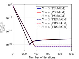
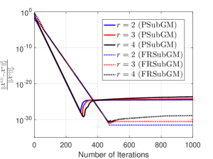
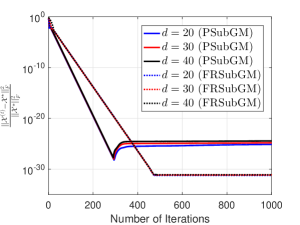
Figure 1: Performance comparison of the PSubGM and FRSubGM in the robust tensor recovery, (a) for different $N$ with $d=6$, $r=2$, $m=1500$, $p_{s}=0.3$, $\lambda=0.5$, $q=0.9$ (PSubGM) and $q=0.91$ (FRSubGM) (b) for different $r$ with $d=40$, $N=3$, $m=12000$, $p_{s}=0.3$, $\lambda=0.5$, $q=0.9$ (PSubGM) and $q=0.93$ (FRSubGM) (c) for different $d$ with $N=3$, $r=2$, $m=3000$, $p_{s}=0.3$, $\lambda=0.5$, $q=0.9$ (PSubGM) and $q=0.93$ (FRSubGM).

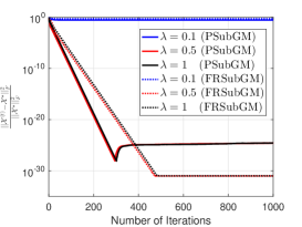
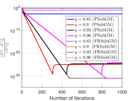
Figure 2: Performance comparison of the PSubGM and FRSubGM in the robust tensor recovery, (a) for different $\lambda$ with $N=3$, $d=30$, $r=2$, $m=2000$, $p_{s}=0.3$, $q=0.9$ (PSubGM) and $q=0.93$ (FRSubGM), (b) for different $q$ with $N=3$, $d=30$, $r=2$, $m=2000$, $p_{s}=0.3$ and $\lambda=0.5$.

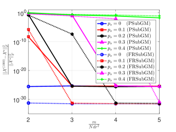
Figure 3: Recovery error of the PSubGM and FRSubGM for different $p_{s}$ and $m$ with $N=3$, $d=10$, $r=2$, $\lambda=0.5$, $q=0.9$ (PSubGM) and $q=0.91$ (FRSubGM).

In the first experiment, we evaluate the performance of PSubGM and FRSubGM in terms of $N$, $d$, and $r$. Figures 1-1 clearly demonstrate that PSubGM exhibits a faster convergence speed compared to FRSubGM. However, the final recovery error of PSubGM is slightly higher than that of FRSubGM, which can possibly be attributed to the sub-optimality of the TT-SVD. Notably, unlike the significantly slower convergence rates of IHT [38] and FRGD [46] as $N$, $r$, and $d$ increase observed from [47, Figure 1], PSubGM and FRSubGM do not exhibit such degradation, attributable to the use of a diminishing step size.

In the second experiment, we test the performance of PSubGM and FRSubGM in terms of $\lambda$ and $q$. In Figures 2 and 2, we can observe that both larger and smaller values of $\lambda$ or $q$ can potentially result in slower convergence or worse recovery error. Therefore, it is crucial to carefully fine-tune the parameters $\lambda$ and $q$ to ensure optimal performance.

In the third experiment, we test the performance of PSubGM and FRSubGM in terms of $p_{s}$ and $m$. Figure 3 illustrates the relationship between recovery error and $p_{s}$ and $m$. It is evident that a larger value of $\frac{m}{Ndr^{2}}$ ensures better performance, as the $\ell_{1}/\ell_{2}$-RIP constant $\delta$ is inversely proportional to $m$. Moreover, as $p_{s}$ increases, a larger number of measurement operators $m$ is required.

In the last experiment, we investigate the necessary value of $m$ for different $N$ utilizing PSubGM and FRSubGM. This investigation is illustrated in Figures 4 and 4, where we evaluate the success rate of achieving $\frac{\|\mathcal{X}^{(1000)}-\mathcal{X}^{\star}\|_{F}^{2}}{\|\mathcal{X}^{\star}\|_{F}^{2}}\leq 10^{-5}$ over $100$ independent trials. Our findings demonstrate a trend: as the value of $m$ increases and $N$ decreases, the success rate of recovery also improves. In addition, we establish a linear correlation between the number of measurements, $m$, and the tensor oders $N$, aligning with the conditions stipulated in Theorem 1. It is important to recognize that FRSubGM necessitates a larger value of $m$ compared to PSubGM. This difference arises from our analysis, where FRSubGM must adhere to the $(N+1)\overline{r}$-$\ell_{1}/\ell_{2}$-RIP, whereas PSubGM only requires the $3\overline{r}$-$\ell_{1}/\ell_{2}$-RIP.

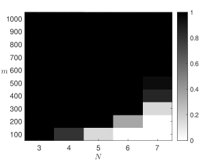
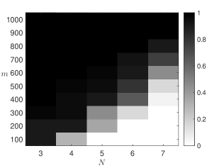
Figure 4: Performance comparison of (a) PSubGM and (b) FRSubGM in the robust tensor recovery, for different $N$ and $m$ with $d=4$, $r=2$, $p_{s}=0.05$, $\lambda=0.07$ and $q=0.99$.

5 Conclusion

In this paper, we develop efficient algorithms with guaranteed performance for robust tensor train (TT) recovery in the presence of outliers. We first prove the $\ell_{1}/\ell_{2}$-RIP of the Gaussian measurement operator and the sharpness property of the robust $\ell_{1}$ loss formulation, implying the possibility of exact recovery even when the measurements are corrupted by outliers. We then propose two iterative algorithms, namely the projected subgradient method (PSubGM) and the factorized Riemannian subgradient method (FRSubGM), to solve the corresponding recovery problems. With suitable initialization and diminishing step sizes, we show that both PSubGM and FRSubGM converge to the ground truth tensor at a linear rate and can tolerate a significant amount of outliers, with the outlier ratio being as large as half. We also demonstrate that a truncated spectral method can provide an appropriate initialization to ensure the local convergence of both algorithms.

As mentioned earlier, the convergence rate of the FRSubGM is influenced by the condition number $\kappa(\mathcal{X}^{\star})$; as $\kappa(\mathcal{X}^{\star})$ increases, the convergence rate becomes slower. In future research, it would be worthwhile to incorporate the scaled technique [77, 45, 54] into our algorithms to mitigate the impact of $\mathcal{X}^{\star}$ on convergence. Another promising avenue for future exploration is the investigation of robust overparameterized TT recovery, building upon the advancements made in the matrix case [78, 79, 80, 81].

Appendix A Technical tools used in proofs

We present some useful results for the proofs in the next sections.

Lemma 6.

([46, Lemma 3]) For any $\bm{A}_{i},\bm{A}^{\star}_{i}\in\mathbb{R}^{r_{i-1}\times r_{i}},i\in[N]$, we have

$$\bm{A}_{1}\bm{A}_{2}\cdots\bm{A}_{N}-\bm{A}_{1}^{\star}\bm{A}_{2}^{\star}\cdots\bm{A}_{N}^{\star}=\sum_{i=1}^{N}\bm{A}_{1}^{\star}\cdots\bm{A}_{i-1}^{\star}(\bm{A}_{i}-\bm{A}_{i}^{\star})\bm{A}_{i+1}\cdots\bm{A}_{N}.$$ (32)

Lemma 7.

Consider the loss function $f(\mathcal{X})=\frac{1}{m}\|\mathcal{A}(\mathcal{X})-\bm{y}\|_{1}$, where the measurement operator $\mathcal{A}$ satisfies the $\ell_{1}/\ell_{2}$-RIP with a constant $\delta_{2\overline{r}}$. Then for any $\mathcal{X}$, it holds that

$$\|\mathcal{D}\|_{F}\leq\sqrt{2/\pi}+\delta_{2\overline{r}},\forall\mathcal{D}\in\partial f(\mathcal{X}).$$ (33)

Proof.

Recall the definition of (Fr$\rm\acute{e}$chet) subdifferential [34] of $f$ at $\mathcal{X}$

$$\partial f(\mathcal{X})=\bigg{\{}\mathcal{D}\in\mathbb{R}^{d_{1}\times\cdots\times d_{N}}:\liminf_{\mathcal{X}^{\prime}\to\mathcal{X}}\frac{f(\mathcal{X}^{\prime})-f(\mathcal{X})-\langle\mathcal{D},\mathcal{X}^{\prime}-\mathcal{X}\rangle}{\|\mathcal{X}^{\prime}-\mathcal{X}\|_{F}}\geq 0\bigg{\}},$$ (34)

where each $\mathcal{D}\in\partial f(\mathcal{X})$ is called a subgradient of $f$ at $\mathcal{X}$.

Now for any $\mathcal{X}^{\prime}\in\mathbb{R}^{d_{1}\times\cdots\times d_{N}}$, we have

$$|f(\mathcal{X}^{\prime})-f(\mathcal{X})| \!\!\!\!=\!\!\!\! \frac{1}{m}\big{|}\|\mathcal{A}(\mathcal{X}^{\prime})-\bm{y}\|_{1}-\|\mathcal{A}(\mathcal{X})-\bm{y}\|_{1}\big{|}$$ (35)

$$\!\!\!\!\leq\!\!\!\! \frac{1}{m}\|\mathcal{A}(\mathcal{X}^{\prime}-\mathcal{X})\|_{1}$$

$$\!\!\!\!\leq\!\!\!\! (\sqrt{2/\pi}+\delta_{2\overline{r}})\|\mathcal{X}^{\prime}-\mathcal{X}\|_{F},$$

where the second inequality follows from the $\ell_{1}/\ell_{2}$-RIP of $\mathcal{A}$. This further implies that

$$\liminf_{\mathcal{X}^{\prime}\to\mathcal{X}}\frac{|f(\mathcal{X}^{\prime})-f(\mathcal{X})|}{\|\mathcal{X}^{\prime}-\mathcal{X}\|_{F}}\leq\lim_{\mathcal{X}^{\prime}\to\mathcal{X}}\frac{(\sqrt{2/\pi}+\delta_{2\overline{r}})\|\mathcal{X}^{\prime}-\mathcal{X}\|_{F}}{\|\mathcal{X}^{\prime}-\mathcal{X}\|_{F}}=\sqrt{2/\pi}+\delta_{2\overline{r}}.$$ (36)

Upon taking $\mathcal{X}^{\prime}=\mathcal{X}+t\mathcal{D},t\to 0$ and invoking (34), we have

$$\|\mathcal{D}\|_{F}\leq\sqrt{2/\pi}+\delta_{2\overline{r}},\ \ \forall\mathcal{D}\in\partial f(\mathcal{X}).$$ (37)

∎

Lemma 8.

([82, Lemma 1]) Let $\bm{X}^{\top}\bm{X}={\bf I}$ and ${\bm{\xi}}$ on the tangent space of Stiefel manifold be given. Consider the point ${\bm{X}}^{+}={\bm{X}}+{\bm{\xi}}$. Then, the polar decomposition-based retraction satisfies $\text{Retr}_{\bm{X}}({\bm{X}}^{+})={\bm{X}}^{+}({{\bm{X}}^{+}}^{\top}{\bm{X}}^{+})^{-\frac{1}{2}}$ and

$$\|\text{Retr}_{\bm{X}}(\bm{X}^{+})-\overline{\bm{X}}\|_{F}\leq\|{\bm{X}}^{+}-\overline{\bm{X}}\|_{F}=\|{\bm{X}}+{\bm{\xi}}-\overline{\bm{X}}\|_{F}$$ (38)

for any $\overline{\bm{X}}^{\top}\overline{\bm{X}}={\bf I}$.

Finally, we introduce a new operation related to the multiplication of submatrices within the left unfolding matrices $L(\bm{X}_{i})=\begin{bmatrix}\bm{X}_{i}^{\top}(1)\cdots\bm{X}_{i}^{\top}(d_{i})\end{bmatrix}^{\top}\in\mathbb{R}^{(r_{i-1}d_{i})\times r_{i}},i\in[N]$. For simplicity, we will only consider the case $d_{i}=2$, but extending to the general case is straightforward. In particular, let $\bm{A}=\begin{bmatrix}\bm{A}_{1}\\ \bm{A}_{2}\end{bmatrix}$ and $\bm{B}=\begin{bmatrix}\bm{B}_{1}\\ \bm{B}_{2}\end{bmatrix}$ be two block matrices, where $\bm{A}_{i}\in\mathbb{R}^{r_{1}\times r_{2}}$ and $\bm{B}_{i}\in\mathbb{R}^{r_{2}\times r_{3}}$ for $i=1,2$. We introduce the notation $\overline{\otimes}$ to represent the Kronecker product between submatrices in the two block matrices, as an alternative to the standard Kronecker product based on element-wise multiplication. Specifically, we define $\bm{A}\overline{\otimes}\bm{B}$ as $\bm{A}\overline{\otimes}\bm{B}=\begin{bmatrix}\bm{A}_{1}\\ \bm{A}_{2}\end{bmatrix}\overline{\otimes}\begin{bmatrix}\bm{B}_{1}\\ \bm{B}_{2}\end{bmatrix}=\begin{bmatrix}(\bm{A}_{1}\bm{B}_{1})^{\top}\ (\bm{A}_{2}\bm{B}_{1})^{\top}\ (\bm{A}_{1}\bm{B}_{2})^{\top}\ (\bm{A}_{2}\bm{B}_{2})^{\top}\end{bmatrix}^{\top}$.

According to [46, Lemma 2], we can conclude that for any left-orthogonal TT format tensor $\mathcal{X}^{\star}=[\bm{X}_{1}^{\star},\dots,\bm{X}_{N}^{\star}]$, we have

$$\|\mathcal{X}^{\star}\|_{F}=\|\text{vec}(\mathcal{X}^{\star})\|_{2}=\|L(\bm{X}_{1}^{\star})\overline{\otimes}\cdots\overline{\otimes}L(\bm{X}_{N}^{\star})\|_{2}=\|L(\bm{X}_{N}^{\star})\|_{2},$$ (39)

$$\|L(\bm{X}_{i}^{\star})\overline{\otimes}\cdots\overline{\otimes}L(\bm{X}_{N-1}^{\star})\overline{\otimes}L(\bm{X}_{N}^{\star})\|_{2}\leq\Pi_{l=i}^{N-1}\|L(\bm{X}_{l}^{\star})\|\|L(\bm{X}_{N}^{\star})\|_{2}=\|L(\bm{X}_{N}^{\star})\|_{2},\ \ \forall i\in[N-1],$$ (40)

$$\|L(\bm{X}_{i}^{\star})\overline{\otimes}\cdots\overline{\otimes}L(\bm{X}_{j}^{\star})\|\leq\Pi_{l=i}^{j}\|L(\bm{X}_{l}^{\star})\|=1,\ \ i\leq j,\ \ \forall i,j\in[N-1],$$ (41)

$$\|L(\bm{X}_{i}^{\star})\overline{\otimes}\cdots\overline{\otimes}L(\bm{X}_{j}^{\star})\|_{F}\leq\Pi_{l=i}^{j-1}\|L(\bm{X}_{l}^{\star})\|\|L(\bm{X}_{j}^{\star})\|_{F},\ \ i\leq j,\ \ \forall i,j\in[N-1].$$ (42)

Appendix B Proof of Theorem 1

Proof.

We first compute the covering number for any low-TT-rank tensor $\mathcal{X}=[\bm{X}_{1},\dots,\bm{X}_{N}]\in\mathbb{R}^{d_{1}\times\cdots\times d_{N}}$ with ranks $(r_{1},\dots,r_{N-1})$. Given that any TT format can be converted to its left-orthogonal form, we denote $\mathcal{X}=[\bm{X}_{1},\dots,\bm{X}_{N}]$ as the left-orthogonal format. According to [83], we can construct $\epsilon$-net $\{L(\bm{X}_{i}^{(1)}),\dots,L(\bm{X}_{i}^{(n_{i})})\},i\in[N-1]$ for each set of matrices $\{L(\bm{X}_{i})\in\mathbb{R}^{d_{i}r_{i-1}\times r_{i}},i\in[N-1]:\|L(\bm{X}_{i})\|\leq 1\}$ ($r_{0}=1$) such that

$$\sup_{L(\bm{X}_{i}):\|L(\bm{X}_{i})\|\leq 1}\min_{p_{i}\leq n_{i}}\|L(\bm{X}_{i})-L(\bm{X}_{i}^{(p_{i})})\|\leq\epsilon,$$ (43)

with the covering number $n_{i}\leq(\frac{4+\epsilon}{\epsilon})^{d_{i}r_{i-1}r_{i}}$. Also, we can construct $\epsilon$-net $\{L(\bm{X}_{N}^{(1)}),\dots,L(\bm{X}_{N}^{(n_{N})})\}$ for $\{L(\bm{X}_{N})\in\mathbb{R}^{d_{N}r_{N-1}\times 1}:\|L(\bm{X}_{N})\|_{2}\leq 1\}$ such that

$$\sup_{L(\bm{X}_{N}):\|L(\bm{X}_{N})\|_{2}\leq 1}\min_{p_{N}\leq n_{N}}\|L(\bm{X}_{N})-L(\bm{X}_{N}^{(p_{N})})\|_{2}\leq\epsilon,$$ (44)

with the covering number $n_{N}\leq(\frac{2+\epsilon}{\epsilon})^{d_{N}r_{N-1}r_{N}}$. Hence, for any low-rank TT format $\mathcal{X}$ with $\|\mathcal{X}\|_{F}\leq\|\bm{X}_{N}\|_{F}\leq 1$ derived from (40), its covering argument is $\Pi_{i=1}^{N}n_{i}\leq(\frac{4+\epsilon}{\epsilon})^{d_{1}r_{1}+\sum_{i=2}^{N-1}d_{i}r_{i-1}r_{i}+d_{N}r_{N-1}}\leq(\frac{4+\epsilon}{\epsilon})^{N\overline{d}\overline{r}^{2}}$ where $\overline{r}=\max_{i}r_{i}$ and $\overline{d}=\max_{i}d_{i}$.

Without loss of the generality, we assume that $\mathcal{X}$ is in TT format with $\|\mathcal{X}\|_{F}=1$. For simplicity, we use $\mathcal{I}$ to denote the index set $[n_{1}]\times\cdots\times[n_{N}]$. According to the construction of the $\epsilon$-net, there exists $p=(p_{1},\dots,p_{N})\in\mathcal{I}$ such that

$$\|L(\bm{X}_{i})-L(\bm{X}_{i}^{(p_{i})})\|\leq\epsilon,\ \ i\in[N-1]\ \ \ \text{and}\ \ \ \|L(\bm{X}_{N})-L(\bm{X}_{N}^{(p_{N})})\|_{2}\leq\epsilon.$$ (45)

Taking $\epsilon=\frac{c\delta_{\overline{r}}}{N}$ with a positive constant $c$ gives

$$\sup_{\mathcal{X}}\frac{1}{m}\|\mathcal{A}(\mathcal{X}-\mathcal{X}^{(p)})\|_{1}$$ (46)

$$\!\!\!\!=\!\!\!\! \sup_{[\bm{X}_{1},\dots,\bm{X}_{N}]}\frac{1}{m}\sum_{k=1}^{m}|\langle\mathcal{A}_{k},[\bm{X}_{1},\dots,\bm{X}_{N}]-[\bm{X}_{1}^{(p_{1})},\dots,\bm{X}_{N}^{(p_{N})}]\rangle|$$

$$\!\!\!\!=\!\!\!\! \sup_{[\bm{X}_{1},\dots,\bm{X}_{N}]}\frac{1}{m}\sum_{k=1}^{m}|\langle\mathcal{A}_{k},\sum_{a_{1}=1}^{N}[\bm{X}_{1}^{(p_{1})},\dots,\bm{X}_{a_{1}}^{(p_{a_{1}})}-\bm{X}_{a_{1}},\dots,\bm{X}_{N}]\rangle|$$

$$\!\!\!\!\leq\!\!\!\! \sup_{\mathcal{X}}\frac{N\epsilon}{m}\|\mathcal{A}(\mathcal{X})\|_{1}=\sup_{\mathcal{X}}\frac{c\delta_{\overline{r}}}{m}\|\mathcal{A}(\mathcal{X})\|_{1},$$

where we write $[\bm{X}_{1},\dots,\bm{X}_{N}]-[\bm{X}_{1}^{(p_{1})},\dots,\bm{X}_{N}^{(p_{N})}]$ in the second line as the sum of $N$ terms via Lemma 6.

According to (46), we have

$$\sup_{\mathcal{X}}\bigg{|}\frac{1}{m}\|\mathcal{A}(\mathcal{X})\|_{1}-\sqrt{2/\pi}\bigg{|}$$ (47)

$$\!\!\!\!\leq\!\!\!\! \sup_{\mathcal{X}^{(p)}}\bigg{|}\frac{1}{m}\|\mathcal{A}(\mathcal{X}^{(p)})\|_{1}-\sqrt{2/\pi}\bigg{|}+\sup_{\mathcal{X}}\frac{1}{m}\|\mathcal{A}(\mathcal{X}-\mathcal{X}^{(p)})\|_{1}$$

$$\!\!\!\!\leq\!\!\!\! \sup_{\mathcal{X}^{(p)}}\bigg{|}\frac{1}{m}\|\mathcal{A}(\mathcal{X}^{(p)})\|_{1}-\sqrt{2/\pi}\bigg{|}+\sup_{\mathcal{X}}\frac{c\delta_{\overline{r}}}{m}\|\mathcal{A}(\mathcal{X})\|_{1}$$

$$\!\!\!\!\leq\!\!\!\! \sup_{\mathcal{X}^{(p)}}\bigg{|}\frac{1}{m}\|\mathcal{A}(\mathcal{X}^{(p)})\|_{1}-\sqrt{2/\pi}\bigg{|}+\sup_{\mathcal{X}}c\delta_{\overline{r}}\bigg{|}\frac{1}{m}\|\mathcal{A}(\mathcal{X})\|_{1}-\sqrt{2/\pi}\bigg{|}+c\delta_{\overline{r}}\sqrt{2/\pi},$$

and then it follows

$$\sup_{\mathcal{X}}\bigg{|}\frac{1}{m}\|\mathcal{A}(\mathcal{X})\|_{1}-\sqrt{2/\pi}\bigg{|}\leq\frac{\sup_{\mathcal{X}^{(p)}}\bigg{|}\frac{1}{m}\|\mathcal{A}(\mathcal{X}^{(p)})\|_{1}-\sqrt{2/\pi}\bigg{|}+c\delta_{\overline{r}}\sqrt{2/\pi}}{1-c\delta_{\overline{r}}}.$$ (48)

To finish our derivation, we need to obtain the concentration inequality with respect to $\frac{1}{m}\sum_{k=1}^{m}|\langle\mathcal{A}_{k},\mathcal{X}^{(p)}\rangle|$. For any fixed TT format tensor $\mathcal{X}^{(p)}$ with $\|\mathcal{X}^{(p)}\|_{F}=1$, $|\langle\mathcal{A}_{k},\mathcal{X}^{(p)}\rangle|$ obeys standard Gaussian with mean $\sqrt{2/\pi}$ and unit variance since $\{\mathcal{A}_{k}\}_{k=1}^{m}$ have i.i.d. standard Gaussian entries. Hence, based on the tail function of Gaussian random variable, we have

$$\operatorname{\mathbb{P}}\left(\sup_{\mathcal{X}^{(p)}}\bigg{|}\frac{1}{m}\sum_{k=1}^{m}|\langle\mathcal{A}_{k},\mathcal{X}^{(p)}\rangle|-\sqrt{2/\pi}\bigg{|}\geq\frac{\delta_{\overline{r}}}{2}\right)\leq 2e^{-c_{1}m\delta_{\overline{r}}^{2}},$$ (49)

where $c_{1}$ is a constant.

Based on (48), we can derive

$$\operatorname{\mathbb{P}}\left(\sup_{\mathcal{X}}\bigg{|}\frac{1}{m}\|\mathcal{A}(\mathcal{X})\|_{1}-\sqrt{2/\pi}\bigg{|}\geq\frac{\frac{\delta_{\overline{r}}}{2}+c\delta_{\overline{r}}\sqrt{2/\pi}}{1-c\delta_{\overline{r}}}\right)$$ (50)

$$\!\!\!\!\leq\!\!\!\! \operatorname{\mathbb{P}}\left(\frac{\sup_{\mathcal{X}^{(p)}}\bigg{|}\frac{1}{m}\|\mathcal{A}(\mathcal{X}^{(p)})\|_{1}-\sqrt{2/\pi}\bigg{|}+c\delta_{\overline{r}}\sqrt{2/\pi}}{1-c\delta_{\overline{r}}}\geq\frac{\frac{\delta_{\overline{r}}}{2}+c\delta_{\overline{r}}\sqrt{2/\pi}}{1-c\delta_{\overline{r}}}\right)$$

$$\!\!\!\!\leq\!\!\!\! \Pi_{i=1}^{N}n_{i}e^{1-c_{1}m\delta_{\overline{r}}^{2}}$$

$$\!\!\!\!\leq\!\!\!\! \bigg{(}\frac{4+\epsilon}{\epsilon}\bigg{)}^{N\overline{d}\overline{r}^{2}}e^{1-c_{1}m\delta_{\overline{r}}^{2}}$$

$$\!\!\!\!\leq\!\!\!\! e^{1-c_{1}m\delta_{\overline{r}}^{2}+c_{2}N\overline{d}\overline{r}^{2}\log N},$$

where in the last line, we choose $\epsilon=\frac{c\delta_{\overline{r}}}{N}$, and $c_{2}$ is a positive constant. Based on (50), we have

$$\operatorname{\mathbb{P}}\left(\sup_{\mathcal{X}}\bigg{|}\frac{1}{m}\|\mathcal{A}(\mathcal{X})\|_{1}-\sqrt{2/\pi}\bigg{|}\leq\frac{\frac{\delta_{\overline{r}}}{2}+c\delta_{\overline{r}}\sqrt{2/\pi}}{1-c\delta_{\overline{r}}}\right)\geq 1-e^{1-c_{1}m\delta_{\overline{r}}^{2}+c_{2}N\overline{d}\overline{r}^{2}\log N}.$$ (51)

To guarantee that $\frac{\frac{\delta_{\overline{r}}}{2}+c\delta_{\overline{r}}\sqrt{2/\pi}}{1-c\delta_{\overline{r}}}\leq\delta_{\overline{r}}\leq\sqrt{2/\pi}$, we can select $c=\frac{\sqrt{2\pi}}{8}$ in $\epsilon=\frac{c\delta_{\overline{r}}}{N}$. Furthermore, if $m\geq\Omega(N\overline{d}\overline{r}^{2}\log N/\delta_{\overline{r}}^{2})$, we obtain the following result:

$$\operatorname{\mathbb{P}}\left(\sup_{\mathcal{X}}\bigg{|}\frac{1}{m}\|\mathcal{A}(\mathcal{X})\|_{1}-\sqrt{2/\pi}\bigg{|}\leq\delta_{\overline{r}}\right)\geq 1-e^{-c_{3}N\overline{d}\overline{r}^{2}\log N},$$ (52)

where $c_{3}$ is a constant. In other words, with probability at least $1-e^{-c_{3}N\overline{d}\overline{r}^{2}\log N}$, it holds that

$$(\sqrt{2/\pi}-\delta_{\overline{r}})\|\mathcal{X}\|_{F}\leq\frac{1}{m}\|\mathcal{A}(\mathcal{X})\|_{1}\leq(\sqrt{2/\pi}+\delta_{\overline{r}})\|\mathcal{X}\|_{F}$$ (53)

for any low-TT-rank tensor $\mathcal{X}\in\mathbb{R}^{d_{1}\times\cdots\times d_{N}}$ with ranks $(r_{1},\dots,r_{N-1})$.

∎

Appendix C Proof of Lemma 1

Proof.

We first expand $\frac{1}{m}\|\mathcal{A}(\mathcal{X}-\mathcal{X}^{\star})-\bm{s}\|_{1}-\frac{1}{m}\|\bm{s}\|_{1}$ as

$$\frac{1}{m}\|\mathcal{A}(\mathcal{X}-\mathcal{X}^{\star})-\bm{s}\|_{1}-\frac{1}{m}\|\bm{s}\|_{1}$$ (54)

$$\!\!\!\!=\!\!\!\! \frac{1}{m}\|\mathcal{A}_{\mathcal{S}^{c}}(\mathcal{X}-\mathcal{X}^{\star})\|_{1}+\frac{1}{m}\|\mathcal{A}_{\mathcal{S}}(\mathcal{X}-\mathcal{X}^{\star})-\bm{s}\|_{1}-\frac{1}{m}\|\bm{s}\|_{1}$$

$$\!\!\!\!\geq\!\!\!\! \frac{1}{m}\|\mathcal{A}_{\mathcal{S}^{c}}(\mathcal{X}-\mathcal{X}^{\star})\|_{1}-\frac{1}{m}\|\mathcal{A}_{\mathcal{S}}(\mathcal{X}-\mathcal{X}^{\star})\|_{1}.$$

In the subsequent part, we focus on analyzing the lower bound of $\frac{1}{m}\|\mathcal{A}_{\mathcal{S}^{c}}(\mathcal{X})\|_{1}-\frac{1}{m}\|\mathcal{A}_{\mathcal{S}}(\mathcal{X})\|_{1}$ for any tensor $\mathcal{X}$ in TT format with TT ranks smaller than $2\overline{r}$. We can construct an $\epsilon$-net $\{\mathcal{X}^{(p)}\}$ with the covering number $(\frac{4+\epsilon}{\epsilon})^{4N\overline{d}\overline{r}^{2}}$ for any low-TT-rank tensor $\mathcal{X}$ with ranks $(2r_{1},\dots,2r_{N-1})$ such that (46) holds. Without loss of the generality, we assume that $\mathcal{X}=[\bm{X}_{1},\dots,\bm{X}_{N}]$ is in left-orthogonal TT format with $\|\mathcal{X}\|_{F}=1$. Then we define

$$Y_{k}=\begin{cases}-|\langle\mathcal{A}_{k},\mathcal{X}^{(p)}\rangle|+\sqrt{2/\pi},&k\in\mathcal{S},\\ |\langle\mathcal{A}_{k},\mathcal{X}^{(p)}\rangle|-\sqrt{2/\pi},&k\in\mathcal{S}^{c}.\end{cases}$$ (55)

Hoeffding inequality for Gaussian random variables tells that

$$\operatorname{\mathbb{P}}\left(\frac{1}{m}\sum_{k=1}^{m}Y_{k}=\frac{1}{m}\|\mathcal{A}_{\mathcal{S}^{c}}(\mathcal{X}^{(p)})\|_{1}-\frac{1}{m}\|\mathcal{A}_{\mathcal{S}}(\mathcal{X}^{(p)})\|_{1}-(1-2p_{s})\sqrt{2/\pi}\geq-\frac{\delta_{2\overline{r}}}{2}\right)\geq 1-e^{-c_{1}m\delta_{2\overline{r}}^{2}},$$ (56)

where $c_{1}$ is a constant.

On the other hand, $\frac{1}{m}\|\mathcal{A}_{\mathcal{S}^{c}}(\mathcal{X})\|_{1}\geq\frac{1}{m}\|\mathcal{A}_{\mathcal{S}^{c}}(\mathcal{X}^{(p)})\|_{1}-\frac{1}{m}\|\mathcal{A}_{\mathcal{S}^{c}}(\mathcal{X}-\mathcal{X}^{(p)})\|_{1}$ and $\frac{1}{m}\|\mathcal{A}_{\mathcal{S}}(\mathcal{X})\|_{1}\leq\frac{1}{m}\|\mathcal{A}_{\mathcal{S}}(\mathcal{X}^{(p)})\|_{1}+\frac{1}{m}\|\mathcal{A}_{\mathcal{S}}(\mathcal{X}-\mathcal{X}^{(p)})\|_{1}$ hold for any tensor $\mathcal{X}$. Hence, we have

$$\frac{1}{m}\|\mathcal{A}_{\mathcal{S}^{c}}(\mathcal{X})\|_{1}-\frac{1}{m}\|\mathcal{A}_{\mathcal{S}}(\mathcal{X})\|_{1}\geq\frac{1}{m}\|\mathcal{A}_{\mathcal{S}^{c}}(\mathcal{X}^{(p)})\|_{1}-\frac{1}{m}\|\mathcal{A}_{\mathcal{S}}(\mathcal{X}^{(p)})\|_{1}-\frac{1}{m}\|\mathcal{A}(\mathcal{X}-\mathcal{X}^{(p)})\|_{1}.$$ (57)

Combing (46), we can get

$$\inf_{\mathcal{X}}\bigg{(}\frac{1}{m}\|\mathcal{A}_{\mathcal{S}^{c}}(\mathcal{X})\|_{1}-\frac{1}{m}\|\mathcal{A}_{\mathcal{S}}(\mathcal{X})\|_{1}\bigg{)}$$ (58)

$$\!\!\!\!\geq\!\!\!\! \inf_{\mathcal{X}^{(p)}}\bigg{(}\frac{1}{m}\|\mathcal{A}_{\mathcal{S}^{c}}(\mathcal{X}^{(p)})\|_{1}-\frac{1}{m}\|\mathcal{A}_{\mathcal{S}}(\mathcal{X}^{(p)})\|_{1}\bigg{)}-\sup_{\mathcal{X}}\frac{1}{m}\|\mathcal{A}(\mathcal{X}-\mathcal{X}^{(p)})\|_{1}$$

$$\!\!\!\!\geq\!\!\!\! \inf_{\mathcal{X}^{(p)}}\bigg{(}\frac{1}{m}\|\mathcal{A}_{\mathcal{S}^{c}}(\mathcal{X}^{(p)})\|_{1}-\frac{1}{m}\|\mathcal{A}_{\mathcal{S}}(\mathcal{X}^{(p)})\|_{1}\bigg{)}-\sup_{\mathcal{X}}\frac{c\delta_{2\overline{r}}}{m}\|\mathcal{A}(\mathcal{X})\|_{1}$$

$$\!\!\!\!\geq\!\!\!\! \inf_{\mathcal{X}^{(p)}}\bigg{(}\frac{1}{m}\|\mathcal{A}_{\mathcal{S}^{c}}(\mathcal{X}^{(p)})\|_{1}-\frac{1}{m}\|\mathcal{A}_{\mathcal{S}}(\mathcal{X}^{(p)})\|_{1}\bigg{)}-c\delta_{2\overline{r}}\bigg{(}\frac{\delta_{2\overline{r}}/2+c\delta_{2\overline{r}}\sqrt{2/\pi}}{1-c\delta_{2\overline{r}}}+\sqrt{2/\pi}\bigg{)},$$

where the last line follows the (51) with probability $1-e^{-c_{2}N\overline{d}\overline{r}^{2}\log N}$ in which $c_{2}$ is a positive constant. Denote the event $F:=\{\text{\eqref{Rip conclusion 1} is satisfied}\}$ which holds with probability $1-e^{-c_{2}N\overline{d}\overline{r}^{2}\log N}$. We can take the union bound with (56) to conclude

$$\operatorname{\mathbb{P}}\left(\inf_{\mathcal{X}}\bigg{(}\frac{1}{m}\|\mathcal{A}_{\mathcal{S}^{c}}(\mathcal{X})\|_{1}-\frac{1}{m}\|\mathcal{A}_{\mathcal{S}}(\mathcal{X})\|_{1}\bigg{)}\geq(1-2p_{s})\sqrt{2/\pi}-\frac{\delta_{2\overline{r}}}{2}-c\delta_{2\overline{r}}\bigg{(}\frac{\delta_{2\overline{r}}/2+c\delta_{2\overline{r}}\sqrt{2/\pi}}{1-c\delta_{2\overline{r}}}+\sqrt{2/\pi}\bigg{)}\bigg{|}F\right)$$ (59)

$$\!\!\!\!\geq\!\!\!\! 1-\Pi_{i=1}^{N}n_{i}2e^{c_{1}m\delta_{2\overline{r}}^{2}}$$

$$\!\!\!\!\geq\!\!\!\! 1-(\frac{4+\epsilon}{\epsilon})^{4N\overline{d}\overline{r}^{2}}e^{1-c_{1}m\delta_{2\overline{r}}^{2}}$$

$$\!\!\!\!\geq\!\!\!\! 1-e^{1-c_{1}m\delta_{2\overline{r}}^{2}+c_{3}N\overline{d}\overline{r}^{2}\log N},$$

where $c_{3}$ is a positive constant.

To guarantee that $-\frac{\delta_{2\overline{r}}}{2}-c\delta_{2\overline{r}}(\frac{\delta_{2\overline{r}}/2+c\delta_{2\overline{r}}\sqrt{2/\pi}}{1-c\delta_{2\overline{r}}}+\sqrt{2/\pi})\geq-\delta_{2\overline{r}}$ and $\delta_{2\overline{r}}\leq\sqrt{2/\pi}$, we set $c=\frac{\sqrt{2\pi}}{8}$. While $m\geq\Omega(N\overline{d}\overline{r}^{2}\log N/\delta_{2\overline{r}}^{2})$, we can obtain

$$\operatorname{\mathbb{P}}\left(\inf_{\mathcal{X}}\big{(}\frac{1}{m}\|\mathcal{A}_{\mathcal{S}^{c}}(\mathcal{X})\|_{1}-\frac{1}{m}\|\mathcal{A}_{\mathcal{S}}(\mathcal{X})\|_{1}\big{)}\geq(1-2p_{s})\sqrt{2/\pi}-\delta_{2\overline{r}}\bigg{|}F\right)\geq 1-e^{-c_{4}N\overline{d}\overline{r}^{2}\log N},$$ (60)

where $c_{4}$ is a constant.

In the end, we can derive

$$\operatorname{\mathbb{P}}\left(\inf_{\mathcal{X}}\big{(}\frac{1}{m}\|\mathcal{A}_{\mathcal{S}^{c}}(\mathcal{X})\|_{1}-\frac{1}{m}\|\mathcal{A}_{\mathcal{S}}(\mathcal{X})\|_{1}\big{)}\geq(1-2p_{s})\sqrt{2/\pi}-\delta_{2\overline{r}}\right)$$ (61)

$$\!\!\!\!\geq\!\!\!\! \operatorname{\mathbb{P}}\left(\inf_{\mathcal{X}}\big{(}\frac{1}{m}\|\mathcal{A}_{\mathcal{S}^{c}}(\mathcal{X})\|_{1}-\frac{1}{m}\|\mathcal{A}_{\mathcal{S}}(\mathcal{X})\|_{1}\big{)}\geq(1-2p_{s})\sqrt{2/\pi}-\delta_{2\overline{r}}\cap F\right)$$

$$\!\!\!\!=\!\!\!\! \operatorname{\mathbb{P}}\left(F\right)\operatorname{\mathbb{P}}\left(\inf_{\mathcal{X}}\big{(}\frac{1}{m}\|\mathcal{A}_{\mathcal{S}^{c}}(\mathcal{X})\|_{1}-\frac{1}{m}\|\mathcal{A}_{\mathcal{S}}(\mathcal{X})\|_{1}\big{)}\geq(1-2p_{s})\sqrt{2/\pi}-\delta_{2\overline{r}}\bigg{|}F\right)$$

$$\!\!\!\!\geq\!\!\!\! (1-e^{-c_{2}N\overline{d}\overline{r}^{2}\log N})(1-e^{-c_{4}N\overline{d}\overline{r}^{2}\log N})\geq 1-2e^{-c_{5}N\overline{d}\overline{r}^{2}\log N},$$

where $c_{5}$ is a positive constant. ∎

Appendix D Proof of Lemma 3

Proof.

We can apply the norm inequalities to derive

$$\langle\partial f(\mathcal{X}),\mathcal{X}-\mathcal{X}^{\star}\rangle \!\!\!\!=\!\!\!\! \frac{1}{m}\sum_{k=1}^{m}\text{sign}(\langle\mathcal{A}_{k},\mathcal{X}\rangle-y_{k})(\langle\mathcal{A}_{k},\mathcal{X}-\mathcal{X}^{\star}\rangle-s_{k})+\frac{1}{m}\sum_{k=1}^{m}\text{sign}(\langle\mathcal{A}_{k},\mathcal{X}\rangle-y_{k})s_{k}$$ (62)

$$\!\!\!\!\geq\!\!\!\! \frac{1}{m}\|\mathcal{A}(\mathcal{X}-\mathcal{X}^{\star})-\bm{s}\|_{1}-\frac{1}{m}\|\bm{s}\|_{1}$$

$$\!\!\!\!\geq\!\!\!\! ((1-2p_{s})\sqrt{2/\pi}-\delta_{2\overline{r}})\|\mathcal{X}-\mathcal{X}^{\star}\|_{F},$$

where the last line follows Lemma 1 for $\delta_{2\overline{r}}\leq(1-2p_{s})\sqrt{2/\pi}$.

∎

Appendix E Proof of Theorem 2

Proof.

We expand $\|\mathcal{X}^{(t+1)}-\mathcal{X}^{\star}\|_{F}^{2}$ as following:

$$\|\mathcal{X}^{(t+1)}-\mathcal{X}^{\star}\|_{F}^{2}=\|\text{SVD}_{\bm{r}}^{tt}(\mathcal{X}^{(t)}-\mu_{t}\partial f(\mathcal{X}^{(t)}))-\mathcal{X}^{\star}\|_{F}^{2}$$ (63)

$$\!\!\!\!\leq\!\!\!\! \bigg{(}1+\frac{600N}{\underline{\sigma}({\mathcal{X}^{\star}})}\|\mathcal{X}^{(0)}-\mathcal{X}^{\star}\|_{F}\bigg{)}\|\mathcal{X}^{(t)}-\mu_{t}\partial f(\mathcal{X}^{(t)})-\mathcal{X}^{\star}\|_{F}^{2}$$

$$\!\!\!\!=\!\!\!\! \bigg{(}1+\frac{600N}{\underline{\sigma}({\mathcal{X}^{\star}})}\|\mathcal{X}^{(0)}-\mathcal{X}^{\star}\|_{F}\bigg{)}\big{(}\|\mathcal{X}^{(t)}-\mathcal{X}^{\star}\|_{F}^{2}-2\mu_{t}\langle\partial f(\mathcal{X}^{(t)}),\mathcal{X}^{(t)}-\mathcal{X}^{\star}\rangle+\mu_{t}^{2}\|\partial f(\mathcal{X}^{(t)})\|_{F}^{2}\big{)}$$

$$\!\!\!\!\leq\!\!\!\! \bigg{(}1+\frac{600N}{\underline{\sigma}({\mathcal{X}^{\star}})}\|\mathcal{X}^{(0)}-\mathcal{X}^{\star}\|_{F}\bigg{)}\big{(}\|\mathcal{X}^{(t)}-\mathcal{X}^{\star}\|_{F}^{2}-2\mu_{t}((1-2p_{s})\sqrt{2/\pi}-\delta_{2\overline{r}})\|\mathcal{X}^{(t)}-\mathcal{X}^{\star}\|_{F}$$

$$+\mu_{t}^{2}(\sqrt{2/\pi}+\delta_{2\overline{r}})^{2}\big{)},$$

where we use Lemma 2 in the first inequality and subsequently employ Lemma 3 and Lemma 7 in the last line.

Under the initial condition $\|\mathcal{X}^{(0)}-\mathcal{X}^{\star}\|_{F}\leq\frac{c\underline{\sigma}({\mathcal{X}^{\star}})}{600N}$ with a constant $c$, (63) can be rewritten as

$$\|\mathcal{X}^{(t+1)}-\mathcal{X}^{\star}\|_{F}^{2}\leq(1+c)\big{(}\|\mathcal{X}^{(t)}-\mathcal{X}^{\star}\|_{F}^{2}-2\mu_{t}((1-2p_{s})\sqrt{2/\pi}-\delta_{2\overline{r}})\|\mathcal{X}^{(t)}-\mathcal{X}^{\star}\|_{F}+\mu_{t}^{2}(\sqrt{2/\pi}+\delta_{2\overline{r}})^{2}\big{)}.$$ (64)

Based on the discussion in Appendix E.1, we can select $\mu_{t}=\lambda q^{t}$ where $\lambda=\frac{((1-2p_{s})\sqrt{2/\pi}-\delta_{2\overline{r}})}{2(\sqrt{2/\pi}+\delta_{2\overline{r}})^{2}}\|\mathcal{X}^{(0)}-\mathcal{X}^{\star}\|_{F}$ and $q=\sqrt{(1+c)(1-\frac{3((1-2p_{s})\sqrt{2/\pi}-\delta_{2\overline{r}})^{2}}{4(\sqrt{2/\pi}+\delta_{2\overline{r}})^{2}})}$, and then obtain

$$\|\mathcal{X}^{(t)}-\mathcal{X}^{\star}\|_{F}^{2}\leq\|\mathcal{X}^{(0)}-\mathcal{X}^{\star}\|_{F}^{2}q^{2t}.$$ (65)

∎

E.1 Proof of (65)

Proof.

Define

$$c_{1}=2((1-2p_{s})\sqrt{2/\pi}-\delta_{2\overline{r}}),$$ (66)

$$c_{2}=(\sqrt{2/\pi}+\delta_{2\overline{r}})^{2}.$$ (67)

Now we can simplify (64) as

$$\|\mathcal{X}^{(t+1)}-\mathcal{X}^{\star}\|_{F}^{2}\leq(1+c)(\|\mathcal{X}^{(t)}-\mathcal{X}^{\star}\|_{F}^{2}-\mu_{t}c_{1}\|\mathcal{X}^{(t)}-\mathcal{X}^{\star}\|_{F}+\mu_{t}^{2}c_{2}).$$ (68)

Next, we aim to show

$$\|\mathcal{X}^{(t)}-\mathcal{X}^{\star}\|_{F}\leq c_{0}q^{\frac{t}{2}}=c_{0}(1+c)^{\frac{t}{2}}p^{\frac{t}{2}}$$ (69)

where $c_{0}=\|\mathcal{X}^{(0)}-\mathcal{X}^{\star}\|_{F}$ and $p$ is a parameter that needs to be determined. Let us therefore fix a value $x\in[0,1]$ satisfying $\|\mathcal{X}^{(t)}-\mathcal{X}^{\star}\|_{F}=xc_{0}(1+c)^{\frac{t}{2}}p^{\frac{t}{2}}$. Assume the above induction hypothesis (69) holds at the $t$-iteration. We need to further prove

$$\|\mathcal{X}^{(t+1)}-\mathcal{X}^{\star}\|_{F}^{2}\leq(1+c)\big{(}c_{0}^{2}(1+c)^{t}p^{t}x^{2}-\mu_{t}c_{0}c_{1}(1+c)^{\frac{t}{2}}p^{\frac{t}{2}}x+\mu_{t}^{2}c_{2}\big{)}\leq c_{0}^{2}(1+c)^{t+1}p^{t+1}.$$ (70)

When we select $\mu_{t}=\lambda q^{t}=c_{0}a(1+c)^{\frac{t}{2}}p^{\frac{t}{2}}$ where $a$ is a parameter which needs to be determined, (70) can be simplified as

$$x^{2}-c_{1}ax+c_{2}a^{2}\leq p.$$ (71)

Note that the left hand side of (71) is a convex quadratic in $x$ and therefore the maximum between $[0,1]$ must occur either at $x=0$ or $x=1$.

• When selecting $x=0$, we can derive the condition $c_{2}a^{2}\leq p$.

• When choosing $x=1$, we have $c_{2}a^{2}-c_{1}a+1-p\leq 0$. Since $c_{1},c_{2}>0$, we have $\frac{c_{1}-\sqrt{c_{1}^{2}-4c_{2}(1-p)}}{2c_{2}}\leq a\leq\frac{c_{1}+\sqrt{c_{1}^{2}-4c_{2}(1-p)}}{2c_{2}}$.

By selecting $p=1-\frac{3c_{1}^{2}}{16c_{2}}$ and $a=\frac{c_{1}}{4c_{2}}$, we can ensure that conditions $c_{2}a^{2}\leq p$ and $c_{2}a^{2}-c_{1}a+1-p\leq 0$ holds for $\delta_{2\overline{r}}\geq 0$. Hence we can respectively choose $\lambda=\frac{c_{0}c_{1}}{4c_{2}}$ and $q=\sqrt{(1+c)(1-\frac{3c_{1}^{2}}{16c_{2}})}$, which further guarantees (70).

∎

Appendix F Proof of Lemma 5

Proof.

First, we provide one useful property. According to

$$\text{dist}^{2}(\{\bm{X}_{i}\},\{\bm{X}_{i}^{\star}\})\leq\frac{\underline{\sigma}^{2}(\mathcal{X}^{\star})((1-2p_{s})\sqrt{2/\pi}-\delta_{(N+1)\overline{r}})^{2}}{18(2N^{2}-2N+1)(N+1+\sum_{i=2}^{N-1}r_{i})(\sqrt{2/\pi}+\delta_{(N+1)\overline{r}})^{2}}$$ (72)

which can be obtained by $\mathcal{X}\in\mathcal{C}(b)$ and Lemma 4, we can obtain

$$\sigma_{1}^{2}({\mathcal{X}}^{\langle i\rangle}) \!\!\!\!=\!\!\!\! \|{\mathcal{X}}^{\geq i+1}\|^{2}\leq\min_{\bm{R}_{i}\in\mathbb{O}^{r_{i}\times r_{i}}}2\|\bm{R}_{i}^{\top}{\mathcal{X}^{\star}}^{\geq i+1}\|^{2}+2\|{\mathcal{X}}^{\geq i+1}-\bm{R}_{i}^{\top}{\mathcal{X}^{\star}}^{\geq i+1}\|^{2}$$ (73)

$$\!\!\!\!\leq\!\!\!\! 2\overline{\sigma}^{2}(\mathcal{X}^{\star})+\min_{\bm{R}_{i}\in\mathbb{O}^{r_{i}\times r_{i}}}2\|{\mathcal{X}}^{\langle i\rangle}-{\mathcal{X}^{\star}}^{\langle i\rangle}+{\mathcal{X}^{\star}}^{\langle i\rangle}-{\mathcal{X}}^{\leq i}\bm{R}_{i}^{\top}{\mathcal{X}^{\star}}^{\geq i+1}\|^{2}$$

$$\!\!\!\!\leq\!\!\!\! 2\overline{\sigma}^{2}(\mathcal{X}^{\star})+4\|\mathcal{X}-\mathcal{X}^{\star}\|_{F}^{2}+\min_{\bm{R}_{i}\in\mathbb{O}^{r_{i}\times r_{i}}}4\|\bm{R}_{i}^{\top}{\mathcal{X}^{\star}}^{\geq i+1}\|^{2}\|{\mathcal{X}}^{\leq i}-{\mathcal{X}^{\star}}^{\leq i}\bm{R}_{i}\|_{F}^{2}$$

$$\!\!\!\!\leq\!\!\!\! 2\overline{\sigma}^{2}(\mathcal{X}^{\star})+\bigg{(}4+\frac{16\overline{\sigma}^{2}(\mathcal{X}^{\star})}{\underline{\sigma}^{2}(\mathcal{X}^{\star})}\bigg{)}\|\mathcal{X}-\mathcal{X}^{\star}\|_{F}^{2}$$

$$\!\!\!\!\leq\!\!\!\! 2\overline{\sigma}^{2}(\mathcal{X}^{\star})+\frac{45N\overline{\sigma}^{2}(\mathcal{X}^{\star})}{\underline{\sigma}^{2}(\mathcal{X}^{\star})}\text{dist}^{2}(\{\bm{X}_{i}\},\{\bm{X}_{i}^{\star}\})\leq\frac{9\overline{\sigma}^{2}(\mathcal{X}^{\star})}{4},i\in[N-1],$$

where the fourth and last lines respectively follow [46, eq. (60)] and Lemma 4. Note that $\overline{\sigma}^{2}(\mathcal{X})=\max_{i=1}^{N-1}\sigma_{1}^{2}({\mathcal{X}}^{\langle i\rangle})\leq\frac{9\overline{\sigma}^{2}(\mathcal{X}^{\star})}{4}$.

Then we need to define the subgradient of $F(\bm{X}_{1},\dots,\bm{X}_{N})$ as following:

$$\partial_{L(\bm{X}_{i})}F(\bm{X}_{1},\dots,\bm{X}_{N})=\begin{bmatrix}\partial_{\bm{X}_{i}(1)}F(\bm{X}_{1},\dots,\bm{X}_{N})\\ \vdots\\ \partial_{\bm{X}_{i}(d_{i})}F(\bm{X}_{1},\dots,\bm{X}_{N})\end{bmatrix}.$$ (74)

Here the subgradient with respect to each factor $\bm{X}_{i}(s_{i})$ can be computed as

$$\partial_{\bm{X}_{i}(s_{i})}F(\bm{X}_{1},\dots,\bm{X}_{N})=\frac{1}{m}\sum_{k=1}^{m}\text{sign}(\langle\mathcal{A}_{k},\mathcal{X}\rangle-y_{k})\sum_{s_{1},\ldots,s_{i-1},\atop s_{i+1},\ldots,s_{N}}\Big{(} \mathcal{A}_{k}(s_{1},\dots,s_{N})\bm{X}_{i-1}^{\top}(s_{i-1})\cdots\bm{X}_{1}^{\top}(s_{1})\cdot$$

$$\bm{X}_{N}^{\top}(s_{N})\cdots\bm{X}_{i+1}^{\top}(s_{i+1})\Big{)}.$$

Before analyzing the robust regularity condition, we need to define three matrices for $i\in[N]$ as follows:

$$\bm{D}_{1}(i) \!\!\!\!=\!\!\!\! \begin{bmatrix}\bm{X}_{i-1}^{\top}(1)\!\cdots\!\bm{X}_{1}^{\top}(1)\ \ \ \ \cdots\ \ \ \ \bm{X}_{i-1}^{\top}(d_{i-1})\!\cdots\!\bm{X}_{1}^{\top}(d_{1})\end{bmatrix}$$ (75)

$$\!\!\!\!=\!\!\!\! L^{\top}(\bm{X}_{i-1})\overline{\otimes}\cdots\overline{\otimes}L^{\top}(\bm{X}_{1})\in\mathbb{R}^{r_{i}\times(d_{1}\cdots d_{i-1})},$$

$$\bm{D}_{2}(i) \!\!\!\!=\!\!\!\! \begin{bmatrix}\bm{X}_{N}^{\top}(1)\cdots\bm{X}_{i+1}^{\top}(1)\\ \vdots\\ \bm{X}_{N}^{\top}(d_{N})\cdots\bm{X}_{i+1}^{\top}(d_{i+1})\end{bmatrix}\in\mathbb{R}^{(d_{i+1}\cdots d_{N})\times r_{i}},$$ (76)

where we note that $\bm{D}_{1}(1)=1$ and $\bm{D}_{2}(N)=1$. Moreover, for each $s_{i}\in[d_{i}]$, we define matrix $\bm{E}(s_{i})\in\mathbb{R}^{(d_{1}\cdots d_{i-1})\times(d_{i+1}\cdots d_{N})}$ whose $(s_{1}\cdots s_{i-1},s_{i+1}\cdots s_{N})$-th element is given by

$$\bm{E}(s_{i})(s_{1}\cdots s_{i-1},s_{i+1}\cdots s_{N})=\frac{1}{m}\sum_{k=1}^{m}\text{sign}(\langle\mathcal{A}_{k},\mathcal{X}\rangle-y_{k})\mathcal{A}_{k}(s_{1},\dots,s_{N}).$$ (77)

Based on the aforementioned notations, we can derive

$$\big{\|}\partial_{L(\bm{X}_{i})}F(\bm{X}_{1},\dots,\bm{X}_{N})\big{\|}_{F}^{2} \!\!\!\!=\!\!\!\! \sum_{s_{i}=1}^{d_{i}}\big{\|}\partial_{\bm{X}_{i}(s_{i})}F(\bm{X}_{1},\dots,\bm{X}_{N})\big{\|}_{F}^{2}=\sum_{s_{i}=1}^{d_{i}}\|\bm{D}_{1}(i)\bm{E}(s_{i})\bm{D}_{2}(i)\|_{F}^{2}$$ (78)

$$\!\!\!\!\leq\!\!\!\! \sum_{s_{i}=1}^{d_{i}}\|L^{\top}(\bm{X}_{i-1})\overline{\otimes}\cdots\overline{\otimes}L^{\top}(\bm{X}_{1})\|^{2}\|\bm{D}_{2}(i)\|^{2}\|\bm{E}(s_{i})\|_{F}^{2}$$

$$\!\!\!\!\leq\!\!\!\! \|L(\bm{X}_{1})\|^{2}\cdots\|L(\bm{X}_{i-1})\|^{2}\|{\mathcal{X}}^{\geq i+1}\|^{2}\|\frac{1}{m}\sum_{k=1}^{m}\text{sign}(\langle\mathcal{A}_{k},\mathcal{X}\rangle-y_{k})\mathcal{A}_{k}\|_{F}^{2}$$

$$\!\!\!\!\leq\!\!\!\! \begin{cases}\frac{9\overline{\sigma}^{2}(\mathcal{X}^{\star})}{4}(\sqrt{2/\pi}+\delta_{2\overline{r}})^{2},&i\in[N-1],\\ (\sqrt{2/\pi}+\delta_{2\overline{r}})^{2},&i=N,\end{cases}$$

where we use (41), $\|\bm{D}_{2}(i)\|=\|{\mathcal{X}}^{\geq i+1}\|$ and $\sum_{s_{i}=1}^{d_{i}}\|\bm{E}(s_{i})\|_{F}^{2}=\|\frac{1}{m}\sum_{k=1}^{m}\text{sign}(\langle\mathcal{A}_{k},\mathcal{X}\rangle-y_{k})\mathcal{A}_{k}\|_{F}^{2}$ in the second inequality. In addition, the third inequality follows $\|{\mathcal{X}}^{\geq i+1}\|=\sigma_{1}({\mathcal{X}}^{\langle i\rangle})\leq\frac{3\overline{\sigma}(\mathcal{X}^{\star})}{2}$ and Lemma 7.

Now, we rewrite the cross term in the robust regularity condition as following:

$$\sum_{i=1}^{N}\bigg{\langle}L(\bm{X}_{i})-L_{\bm{R}}(\bm{X}_{i}^{\star}),\mathcal{P}_{\text{T}_{L(\bm{X}_{i})}\text{St}}\big{(}\partial_{L(\bm{X}_{i})}F(\bm{X}_{1},\dots,\bm{X}_{N})\big{)}\bigg{\rangle}$$ (79)

$$\!\!\!\!=\!\!\!\! \sum_{i=1}^{N}\bigg{\langle}L(\bm{X}_{i})-L_{\bm{R}}(\bm{X}_{i}^{\star}),\partial_{L(\bm{X}_{i})}F(\bm{X}_{1},\dots,\bm{X}_{N})\bigg{\rangle}-T$$

$$\!\!\!\!=\!\!\!\! \frac{1}{m}\sum_{k=1}^{m}\text{sign}(\langle\mathcal{A}_{k},\mathcal{X}\rangle-y_{k})\langle\mathcal{A}_{k},\mathcal{X}-\mathcal{X}^{\star}\rangle+\frac{1}{m}\sum_{k=1}^{m}\text{sign}(\langle\mathcal{A}_{k},\mathcal{X}\rangle-y_{k})\langle\text{vec}(\mathcal{A}_{k}),\bm{h}\rangle-T,$$

where

$$\bm{h} \!\!\!\!=\!\!\!\! L_{\bm{R}}(\bm{X}_{1}^{\star})\overline{\otimes}\cdots\overline{\otimes}L_{\bm{R}}({\bm{X}}_{N}^{\star})-L(\bm{X}_{1})\overline{\otimes}\cdots\overline{\otimes}L(\bm{X}_{N-1})\overline{\otimes}L_{\bm{R}}(\bm{X}_{N}^{\star})$$ (80)

$$+\sum_{i=1}^{N-1}L(\bm{X}_{1})\overline{\otimes}\cdots\overline{\otimes}L(\bm{X}_{i-1})\overline{\otimes}(L({\bm{X}}_{i})-L_{\bm{R}}({\bm{X}}_{i}^{\star}))\overline{\otimes}L(\bm{X}_{i+1})\overline{\otimes}\cdots\overline{\otimes}L(\bm{X}_{N}),$$

$$T \!\!\!\!=\!\!\!\! \sum_{i=1}^{N-1}\bigg{\langle}L(\bm{X}_{i})-L_{\bm{R}}(\bm{X}_{i}^{\star}),\mathcal{P}^{\perp}_{\text{T}_{L(\bm{X}_{i})}\text{St}}(\partial_{L(\bm{X}_{i})}F(\bm{X}_{1},\dots,\bm{X}_{N}))\bigg{\rangle}.$$ (81)

To get the lower bound of (79), we need to obtain upper bounds of (80) and (81). According to [46, eq. (82)], we directly obtain

$$\|\bm{h}\|_{2}^{2}\leq\frac{9N(N-1)}{8\overline{\sigma}^{2}(\mathcal{X}^{\star})}\text{dist}^{4}(\{\bm{X}_{i}\},\{\bm{X}_{i}^{\star}\}).$$ (82)

Then, we can derive

$$T \!\!\!\!=\!\!\!\! \sum_{i=1}^{N-1}\bigg{\langle}\mathcal{P}^{\perp}_{\text{T}_{L(\bm{X}_{i})}\text{St}}(L(\bm{X}_{i})-L_{\bm{R}}(\bm{X}_{i}^{\star})),\partial_{L(\bm{X}_{i})}F(\bm{X}_{1},\dots,\bm{X}_{N})\bigg{\rangle}$$ (83)

$$\!\!\!\!\leq\!\!\!\! \frac{1}{2}\sum_{i=1}^{N-1}\|L(\bm{X}_{i})\|\|L(\bm{X}_{i})-L_{\bm{R}}(\bm{X}_{i}^{\star})\|_{F}^{2}\big{\|}\partial_{L(\bm{X}_{i})}F(\bm{X}_{1},\dots,\bm{X}_{N})\big{\|}_{F}$$

$$\!\!\!\!\leq\!\!\!\! \frac{3\overline{\sigma}(\mathcal{X}^{\star})}{4}(\sqrt{2/\pi}+\delta_{2\overline{r}})\sum_{i=1}^{N-1}\|L(\bm{X}_{i})-L_{\bm{R}}(\bm{X}_{i}^{\star})\|_{F}^{2}$$

$$\!\!\!\!\leq\!\!\!\! \frac{3}{4\overline{\sigma}(\mathcal{X}^{\star})}(\sqrt{2/\pi}+\delta_{2\overline{r}})\text{dist}^{2}(\{\bm{X}_{i}\},\{\bm{X}_{i}^{\star}\}),$$

where the first inequality follows (78) and $\mathcal{P}^{\perp}_{\text{T}_{L(\bm{X}_{i})}\text{St}}(\cdot)$ is defined as

$$\mathcal{P}^{\perp}_{\text{T}_{L(\bm{X}_{i})}\text{St}}(L(\bm{X}_{i})-L_{\bm{R}}(\bm{X}_{i}^{\star}))$$ (84)

$$\!\!\!\!=\!\!\!\! L(\bm{X}_{i})-L_{\bm{R}}(\bm{X}_{i}^{\star})-\mathcal{P}_{\text{T}_{L(\bm{X}_{i})}\text{St}}(L(\bm{X}_{i})-L_{\bm{R}}(\bm{X}_{i}^{\star}))$$

$$\!\!\!\!=\!\!\!\! \frac{1}{2}L(\bm{X}_{i})((L(\bm{X}_{i})-L_{\bm{R}}(\bm{X}_{i}^{\star}))^{\top}L(\bm{X}_{i})+L^{\top}(\bm{X}_{i})(L(\bm{X}_{i})-L_{\bm{R}}(\bm{X}_{i}^{\star})))$$

$$\!\!\!\!=\!\!\!\! \frac{1}{2}L(\bm{X}_{i})(2{\bf I}_{r_{i}}-L_{\bm{R}}^{\top}(\bm{X}_{i}^{\star})L(\bm{X}_{i})-L^{\top}(\bm{X}_{i})L_{\bm{R}}(\bm{X}_{i}^{\star}))$$

$$\!\!\!\!=\!\!\!\! \frac{1}{2}L(\bm{X}_{i})((L(\bm{X}_{i})-L_{\bm{R}}(\bm{X}_{i}^{\star}))^{\top}(L(\bm{X}_{i})-L_{\bm{R}}(\bm{X}_{i}^{\star}))).$$

Ultimately, we arrive at

$$\sum_{i=1}^{N}\bigg{\langle}L(\bm{X}_{i})-L_{\bm{R}}(\bm{X}_{i}^{\star}),\mathcal{P}_{\text{T}_{L(\bm{X}_{i})}\text{St}}\big{(}\partial_{L(\bm{X}_{i})}F(\bm{X}_{1},\dots,\bm{X}_{N})\big{)}\bigg{\rangle}$$ (85)

$$\!\!\!\!\geq\!\!\!\! \frac{1}{m}\sum_{k=1}^{m}|\langle\mathcal{A}_{k},\mathcal{X}-\mathcal{X}^{\star}\rangle-s_{k}|-\frac{1}{m}\sum_{k=1}^{m}|s_{k}|-\frac{1}{m}\sum_{k=1}^{m}|\langle\text{vec}(\mathcal{A}_{k}),\bm{h}\rangle|-\frac{3}{4\overline{\sigma}(\mathcal{X}^{\star})}(\sqrt{2/\pi}+\delta_{2\overline{r}})\text{dist}^{2}(\{\bm{X}_{i}\},\{\bm{X}_{i}^{\star}\})$$

$$\!\!\!\!\geq\!\!\!\! ((1-2p_{s})\sqrt{2/\pi}-\delta_{2\overline{r}})\|\mathcal{X}-\mathcal{X}^{\star}\|_{F}-(\sqrt{2/\pi}+\delta_{(N+1)\overline{r}})\|\bm{h}\|_{2}-\frac{3}{4\overline{\sigma}(\mathcal{X}^{\star})}(\sqrt{2/\pi}+\delta_{2\overline{r}})\text{dist}^{2}(\{\bm{X}_{i}\},\{\bm{X}_{i}^{\star}\})$$

$$\!\!\!\!\geq\!\!\!\! \frac{\underline{\sigma}(\mathcal{X}^{\star})((1-2p_{s})\sqrt{2/\pi}-\delta_{(N+1)\overline{r}})}{4\sqrt{2(N+1+\sum_{i=2}^{N-1}r_{i})}\overline{\sigma}(\mathcal{X}^{\star})}\text{dist}(\{\bm{X}_{i}\},\{\bm{X}_{i}^{\star}\})$$

where (83) is used in the first inequality. Note that $\bm{h}$ can be viewed as a TT format where the rank is at most $((N-1)r_{1},\dots,(N-1)r_{N-1})$. Hence, we apply $\ell_{1}/\ell_{2}$-RIP and Lemma 1 in the second inequality. The last line follows $\delta_{2\overline{r}}\leq\delta_{(N+1)\overline{r}}\leq(1-2p_{s})\sqrt{2/\pi}$, (82), Lemma 4 and $\text{dist}^{2}(\{\bm{X}_{i}\},\{\bm{X}_{i}^{\star}\})\leq\frac{\underline{\sigma}^{2}(\mathcal{X}^{\star})((1-2p_{s})\sqrt{2/\pi}-\delta_{(N+1)\overline{r}})^{2}}{18(2N^{2}-2N+1)(N+1+\sum_{i=2}^{N-1}r_{i})(\sqrt{2/\pi}+\delta_{(N+1)\overline{r}})^{2}}$.

∎

Appendix G Proof of Theorem 3

Proof.

To utilize the robust regularity condition of Lemma 5 in the derivation of Theorem 3, we need to prove conditions in Lemma 5. Due to the retraction operation, we can guarantee that $L(\bm{X}_{i}^{(t)})$ are orthonormal. In addition, we assume that

$$\text{dist}^{2}(\{\bm{X}_{i}^{(t)}\},\{\bm{X}_{i}^{\star}\})\leq\frac{\underline{\sigma}^{2}(\mathcal{X}^{\star})((1-2p_{s})\sqrt{2/\pi}-\delta_{(N+1)\overline{r}})^{2}}{18(2N^{2}-2N+1)(N+1+\sum_{i=2}^{N-1}r_{i})(\sqrt{2/\pi}+\delta_{(N+1)\overline{r}})^{2}},$$ (86)

which can be proven later, and following (73), then obtain

$$\sigma_{1}^{2}({\mathcal{X}^{(t)}}^{\langle i\rangle})\leq\frac{9\overline{\sigma}^{2}(\mathcal{X}^{\star})}{4},i\in[N-1].$$ (87)

Next, we define the best rotation matrices as following:

$$(\bm{R}_{1}^{(t)},\dots,\bm{R}_{N-1}^{(t)})=\operatorname*{\text{arg~{}min}}_{\bm{R}_{i}\in\mathbb{O}^{r_{i}\times r_{i}},\atop i\in[N-1]}\sum_{i=1}^{N-1}\overline{\sigma}^{2}(\mathcal{X}^{\star})\|L({\bm{X}}_{i}^{(t)})-L_{\bm{R}}({\bm{X}}_{i}^{\star})\|_{F}^{2}+\|L(\bm{X}_{N}^{(t)})-L_{\bm{R}}({\bm{X}}_{N}^{\star})\|_{2}^{2}.$$ (88)

Now we can prove the assumption $\text{dist}^{2}(\{\bm{X}_{i}^{(t+1)}\},\{\bm{X}_{i}^{\star}\})\leq\text{dist}^{2}(\{\bm{X}_{i}^{(t)}\},\{\bm{X}_{i}^{\star}\})$, expand $\text{dist}^{2}(\{\bm{X}_{i}^{(t+1)}\},\{\bm{X}_{i}^{\star}\})$ and subsequently derive

$$\text{dist}^{2}(\{\bm{X}_{i}^{(t+1)}\},\{\bm{X}_{i}^{\star}\})$$ (89)

$$\!\!\!\!=\!\!\!\! \sum_{i=1}^{N-1}\overline{\sigma}^{2}(\mathcal{X}^{\star})\|L(\bm{X}_{i}^{(t+1)})-L_{\bm{R}^{(t+1)}}(\bm{X}_{i}^{\star})\|_{F}^{2}+\|L(\bm{X}_{N}^{(t+1)})-L_{\bm{R}^{(t+1)}}(\bm{X}_{N}^{\star})\|_{2}^{2}$$

$$\!\!\!\!\leq\!\!\!\! \sum_{i=1}^{N-1}\overline{\sigma}^{2}(\mathcal{X}^{\star})\bigg{\|}L(\bm{X}_{i}^{(t)})-L_{\bm{R}^{(t)}}(\bm{X}_{i}^{\star})-\frac{\mu_{t}}{\overline{\sigma}^{2}(\mathcal{X}^{\star})}\mathcal{P}_{\text{T}_{L({\bm{X}}_{i})}\text{St}}\big{(}\partial_{L({\bm{X}}_{i})}F(\bm{X}_{1}^{(t)},\dots,\bm{X}_{N}^{(t)})\big{)}\bigg{\|}_{F}^{2}$$

$$+\|L(\bm{X}_{N}^{(t)})-L_{\bm{R}^{(t)}}(\bm{X}_{N}^{\star})-\mu_{t}\partial_{L({\bm{X}}_{N})}F(\bm{X}_{1}^{(t)},\dots,\bm{X}_{N}^{(t)})\|_{2}^{2}$$

$$\!\!\!\!=\!\!\!\! \text{dist}^{2}(\{\bm{X}_{i}^{(t)}\},\{\bm{X}_{i}^{\star}\})-2\mu_{t}\sum_{i=1}^{N}\bigg{\langle}L(\bm{X}_{i}^{(t)})-L_{\bm{R}^{(t)}}(\bm{X}_{i}^{\star}),\mathcal{P}_{\text{T}_{L({\bm{X}}_{i})}\text{St}}\big{(}\partial_{L({\bm{X}}_{i})}F(\bm{X}_{1}^{(t)},\dots,\bm{X}_{N}^{(t)})\big{)}\bigg{\rangle}$$

$$+\mu_{t}^{2}\bigg{(}\frac{1}{\overline{\sigma}^{2}(\mathcal{X}^{\star})}\sum_{i=1}^{N-1}\|\mathcal{P}_{\text{T}_{L({\bm{X}}_{i})}\text{St}}\big{(}\partial_{L({\bm{X}}_{i})}F(\bm{X}_{1}^{(t)},\dots,\bm{X}_{N}^{(t)})\big{)}\|_{F}^{2}+\|\partial_{L({\bm{X}}_{N})}F(\bm{X}_{1}^{(t)},\dots,\bm{X}_{N}^{(t)})\|_{2}^{2}\bigg{)},$$

where the first inequality follows the nonexpansiveness property of Lemma 8.

Based on (78), we can easily obtain

$$\frac{1}{\overline{\sigma}^{2}(\mathcal{X}^{\star})}\sum_{i=1}^{N-1}\|\mathcal{P}_{\text{T}_{L({\bm{X}}_{i})}\text{St}}\big{(}\partial_{L(\bm{X}_{i})}F(\bm{X}_{1}^{(t)},\dots,\bm{X}_{N}^{(t)})\big{)}\|_{F}^{2}+\|\partial_{L(\bm{X}_{N})}F(\bm{X}_{1}^{(t)},\dots,\bm{X}_{N}^{(t)})\|_{2}^{2}$$ (90)

$$\!\!\!\!\leq\!\!\!\! \frac{1}{\overline{\sigma}^{2}(\mathcal{X}^{\star})}\sum_{i=1}^{N-1}\|\partial_{L(\bm{X}_{i})}F(\bm{X}_{1}^{(t)},\dots,\bm{X}_{N}^{(t)})\|_{F}^{2}+\|\partial_{L(\bm{X}_{N})}F(\bm{X}_{1}^{(t)},\dots,\bm{X}_{N}^{(t)})\|_{2}^{2}$$

$$\!\!\!\!\leq\!\!\!\! \frac{9N-5}{4}(\sqrt{2/\pi}+\delta_{2\overline{r}})^{2},$$

where the first inequality follows from the fact that for any matrix $\bm{B}=\mathcal{P}_{\text{T}_{L({\bm{X}}_{i})}\text{St}}(\bm{B})+\mathcal{P}_{\text{T}_{L({\bm{X}}_{i})}\text{St}}^{\perp}(\bm{B})$ where $\mathcal{P}_{\text{T}_{L({\bm{X}}_{i})}\text{St}}(\bm{B})$ and $\mathcal{P}_{\text{T}_{L({\bm{X}}_{i})}\text{St}}^{\perp}(\bm{B})$ are orthogonal, we have $\|\mathcal{P}_{\text{T}_{L({\bm{X}}_{i})}\text{St}}(\bm{B})\|_{F}^{2}\leq\|\bm{B}\|_{F}^{2}$.

Hence, combing the robust regularity condition in Lemma 5 and (90), we have

$$\text{dist}^{2}(\{\bm{X}_{i}^{(t+1)}\},\{\bm{X}_{i}^{\star}\}) \!\!\!\!\leq\!\!\!\! \text{dist}^{2}(\{\bm{X}_{i}^{(t)}\},\{\bm{X}_{i}^{\star}\})-\frac{\underline{\sigma}(\mathcal{X}^{\star})((1-2p_{s})\sqrt{2/\pi}-\delta_{(N+1)\overline{r}})}{2\sqrt{2(N+1+\sum_{i=2}^{N-1}r_{i})}\overline{\sigma}(\mathcal{X}^{\star})}\mu_{t}\text{dist}(\{\bm{X}_{i}^{(t)}\},\{\bm{X}_{i}^{\star}\})$$ (91)

$$+\frac{9N-5}{4}(\sqrt{2/\pi}+\delta_{(N+1)\overline{r}})^{2}\mu_{t}^{2}.$$

Following the same analysis of (65) in Appendix E.1, we can set $\mu_{t}=\lambda q^{t}$ where we respectively select

$$\lambda=\frac{(1-2p_{s})\sqrt{2/\pi}-\delta_{(N+1)\overline{r}}}{\sqrt{2(N+1+\sum_{i=2}^{N-1}r_{i})}(9N-5)(\sqrt{2/\pi}+\delta_{(N+1)\overline{r}})^{2}\kappa(\mathcal{X}^{\star})}\text{dist}(\{\bm{X}_{i}^{(0)}\},\{\bm{X}_{i}^{\star}\})$$

and

$$q=\sqrt{1-\frac{((1-2p_{s})\sqrt{2/\pi}-\delta_{(N+1)\overline{r}})^{2}}{8(N+1+\sum_{i=2}^{N-1}r_{i})(9N-5)(\sqrt{2/\pi}+\delta_{(N+1)\overline{r}})^{2}\kappa^{2}(\mathcal{X}^{\star})}},$$

and then guarantee that

$$\text{dist}^{2}(\{\bm{X}_{i}^{(t)}\},\{\bm{X}_{i}^{\star}\})\leq\text{dist}^{2}(\{\bm{X}_{i}^{(0)}\},\{\bm{X}_{i}^{\star}\})q^{2t}.$$ (92)

Proof of (86)

We now prove (86) by induction. First note that (86) holds for $t=0$ which can be proved by combing $\mathcal{X}^{(0)}\in\mathcal{C}(b)$ and Lemma 4. We now assume it holds at $t=t^{\prime}$, which implies that $\sigma_{1}^{2}({\mathcal{X}^{(t^{\prime})}}^{\langle i\rangle})\leq\frac{9\overline{\sigma}^{2}(\mathcal{X}^{\star})}{4},i\in[N-1]$. By invoking (92), we have $\text{dist}^{2}(\{\bm{X}_{i}^{(t^{\prime}+1)}\},\{\bm{X}_{i}^{\star}\})\leq\text{dist}^{2}(\{\bm{X}_{i}^{(t)}\},\{\bm{X}_{i}^{\star}\})$. Consequently, (86) also holds at $t=t^{\prime}+1$. By induction, we can conclude that (86) holds for all $t\geq 0$. This completes the proof.

∎

Appendix H Proof of Theorem 4

Before analyzing the truncated spectral initialization, we first define the following restricted Frobenius norm for any tensor $\mathcal{H}\in\mathbb{R}^{d_{1}\times\cdots\times d_{N}}$:

$$\|\mathcal{H}\|_{F,\overline{r}}=\max_{\mathcal{X}\in\mathbb{R}^{d_{1}\times\cdots\times d_{N}},\|\mathcal{X}\|_{F}\leq 1,\atop{\rm rank}(\mathcal{X})=(r_{1},\dots,r_{N-1})}\langle\mathcal{H},\mathcal{X}\rangle,$$ (93)

where $\operatorname{rank}(\mathcal{X})$ denotes the TT ranks of $\mathcal{X}$.

Following the same analysis of [46, eq. (89)], we have

$$\|\mathcal{X}^{(0)}-\mathcal{X}^{\star}\|_{F} \!\!\!\!\leq\!\!\!\! (1+\sqrt{N-1})\bigg{\|}\frac{1}{(1-p_{s})m}\sum_{k=1}^{m}y_{k}\mathcal{A}_{k}\mathbb{I}_{\{|y_{k}|\leq|\bm{y}|_{(\lceil p_{s}m\rceil)}\}}-\mathcal{X}^{\star}\bigg{\|}_{F,2\overline{r}}$$ (94)

$$\!\!\!\!=\!\!\!\! \max_{\mathcal{X}\in\mathbb{R}^{d_{1}\times\cdots\times d_{N}},\|\mathcal{X}\|_{F}\leq 1,\atop{\rm rank}(\mathcal{X})=(2r_{1},\dots,2r_{N-1})}\frac{1+\sqrt{N-1}}{(1-p_{s})m}\sum_{k\in\mathcal{S}^{\prime}}\big{\langle}y_{k}\mathcal{A}_{k}-\mathcal{X}^{\star},\mathcal{X}\big{\rangle},$$

where $\mathcal{S}^{\prime}=\{k:|y_{k}|\leq|\bm{y}|_{(\lceil p_{s}m\rceil)},k\in[m]\}$ and $|\mathcal{S}^{\prime}|=\lceil(1-p_{s})m\rceil$. Since $|\bm{y}|_{(\lceil p_{s}m\rceil)}\leq\max_{k}|\langle\mathcal{A}_{k},\mathcal{X}^{\star}\rangle|$ where $\langle\mathcal{A}_{k},\mathcal{X}^{\star}\rangle\sim\mathcal{N}(0,\|\mathcal{X}^{\star}\|_{F}^{2})$, we first have

$$\operatorname{\mathbb{P}}\left(|\langle\mathcal{A}_{k},\mathcal{X}^{\star}\rangle|\geq t\right)\leq 2e^{-\frac{t^{2}}{2\|\mathcal{X}^{\star}\|_{F}^{2}}},$$ (95)

and it follows that

$$\operatorname{\mathbb{P}}\left(\max_{k}|\langle\mathcal{A}_{k},\mathcal{X}^{\star}\rangle|\leq t\right) \!\!\!\!\geq\!\!\!\! 1-2\lceil(1-p_{s})m\rceil e^{-\frac{t^{2}}{2\|\mathcal{X}^{\star}\|_{F}^{2}}}$$ (96)

$$\!\!\!\!\geq\!\!\!\! 1-e^{1-\frac{t^{2}}{2\|\mathcal{X}^{\star}\|_{F}^{2}}+\log((1-p_{s})m)}.$$

Then taking $t=c_{1}\|\mathcal{X}^{\star}\|_{F}\log((1-p_{s})m)$ with a positive constant $c_{1}$, with probability $1-e^{-\Omega(\log((1-p_{s})m))}$ we can obtain

$$|\bm{y}|_{(\lceil p_{s}m\rceil)}\leq\max_{k}|\langle\mathcal{A}_{k},\mathcal{X}^{\star}\rangle\leq O(\|\mathcal{X}^{\star}\|_{F}\log((1-p_{s})m)).$$ (97)

Next, according to [46, Appendix E], we can construct an $\epsilon$-net $\{\mathcal{X}^{(1)},\dots,\mathcal{X}^{(p)}\}$ with covering number

$$p\leq(\frac{4+\epsilon}{\epsilon})^{4N\overline{d}\overline{r}^{2}}$$ (98)

for any TT format tensors $\mathcal{X}$ with TT ranks $(2r_{1},\dots,2r_{N-1})$ such that

$$\max_{\mathcal{X}\in\mathbb{R}^{d_{1}\times\cdots\times d_{N}},\|\mathcal{X}\|_{F}\leq 1,\atop{\rm rank}(\mathcal{X})=(2r_{1},\dots,2r_{N-1})}\sum_{k\in\mathcal{S}^{\prime}}\big{\langle}y_{k}\mathcal{A}_{k}-\mathcal{X}^{\star},\mathcal{X}\big{\rangle}\leq 2\sum_{k\in\mathcal{S}^{\prime}}\big{\langle}y_{k}\mathcal{A}_{k}-\mathcal{X}^{\star},\mathcal{X}^{(p)}\big{\rangle}$$ (99)

using $\epsilon=\frac{1}{2N}$.

Note that $\operatorname{\mathbb{E}}_{\mathcal{A}_{k}}\langle y_{k}\mathcal{A}_{k}-\mathcal{X}^{\star},\mathcal{X}^{(p)}\rangle=\operatorname{\mathbb{E}}_{\mathcal{A}_{k}}(\langle\mathcal{A}_{k},\mathcal{X}^{\star}\rangle+s_{k})\langle\mathcal{A}_{k},\mathcal{X}^{(p)}\rangle-\langle\mathcal{X}^{\star},\mathcal{X}^{(p)}\rangle=\langle\mathcal{X}^{\star},\mathcal{X}^{(p)}\rangle-\langle\mathcal{X}^{\star},\mathcal{X}^{(p)}\rangle=0$ since each element in $\mathcal{A}_{k}$ follows the normal distribution. In addition, $\langle y_{k}\mathcal{A}_{k}-\mathcal{X}^{\star},\mathcal{X}^{(p)}\rangle$ is a subgaussian random variable with subgaussian norm $\|\langle y_{k}\mathcal{A}_{k}-\mathcal{X}^{\star},\mathcal{X}^{(p)}\rangle\|_{\psi_{2}}\leq|y_{k}|\|\langle\mathcal{A}_{k},\mathcal{X}^{(p)}\rangle\|_{\psi_{2}}+\|\mathcal{X}^{\star}\|_{F}\|\mathcal{X}^{(p)}\|_{F}\leq O(\log((1-p_{s})m)\|\mathcal{X}^{\star}\|_{F})$ where we use $|y_{k}|\leq|\bm{y}|_{(\lceil p_{s}m\rceil)}\leq O(\|\log((1-p_{s})m)\|\mathcal{X}^{\star}\|_{F})$, $\langle\mathcal{A}_{k},\mathcal{X}^{(p)}\rangle\sim\mathcal{N}(0,\|\mathcal{X}^{(p)}\|_{F}^{2})$ and $\|\mathcal{X}^{(p)}\|_{F}\leq 1$. According to the General Hoeffding’s inequality [62, Theorem 2.6.2], we have

$$\operatorname{\mathbb{P}}\left(|\sum_{k\in\mathcal{S}^{\prime}}\big{\langle}y_{k}\mathcal{A}_{k}-\mathcal{X}^{\star},\mathcal{X}^{(p)}\big{\rangle}|\geq t\right)\leq 2e^{-\frac{c_{2}t^{2}}{(1-p_{s})m(\log((1-p_{s})m))^{2}\|\mathcal{X}^{\star}\|_{F}^{2}}},$$ (100)

where $c_{2}$ is a positive constant. Combing (99) with (100), we further derive

$$\operatorname{\mathbb{P}}\left(\max_{\mathcal{X}\in\mathbb{R}^{d_{1}\times\cdots\times d_{N}},\|\mathcal{X}\|_{F}\leq 1,\atop{\rm rank}(\mathcal{X})=(2r_{1},\dots,2r_{N-1})}\sum_{k\in\mathcal{S}^{\prime}}\big{\langle}y_{k}\mathcal{A}_{k}-\mathcal{X}^{\star},\mathcal{X}\big{\rangle}\geq t\right)$$ (101)

$$\!\!\!\!\leq\!\!\!\! \operatorname{\mathbb{P}}\left(\sum_{k\in\mathcal{S}^{\prime}}\big{\langle}y_{k}\mathcal{A}_{k}-\mathcal{X}^{\star},\mathcal{X}^{(p)}\big{\rangle}\geq\frac{t}{2}\right)$$

$$\!\!\!\!\leq\!\!\!\! \operatorname{\mathbb{P}}\left(|\sum_{k\in\mathcal{S}^{\prime}}\big{\langle}y_{k}\mathcal{A}_{k}-\mathcal{X}^{\star},\mathcal{X}^{(p)}\big{\rangle}|\geq\frac{t}{2}\right)$$

$$\!\!\!\!\leq\!\!\!\! (\frac{4+\epsilon}{\epsilon})^{4N\overline{d}\overline{r}^{2}}e^{1-\frac{c_{2}t^{2}}{4(1-p_{s})m(\log((1-p_{s})m))^{2}\|\mathcal{X}^{\star}\|_{F}^{2}}}$$

$$\!\!\!\!\leq\!\!\!\! e^{1-\frac{c_{2}t^{2}}{4(1-p_{s})m(\log((1-p_{s})m))^{2}\|\mathcal{X}^{\star}\|_{F}^{2}}+c_{3}N\overline{d}\overline{r}^{2}\log N},$$

where $c_{3}$ is a constant and based on the assumption in (99), $\frac{4+\epsilon}{\epsilon}=\frac{4+\frac{1}{2N}}{\frac{1}{2N}}=8N+1$.

Taking $t=\log((1-p_{s})m)\|\mathcal{X}^{\star}\|_{F}\sqrt{(1-p_{s})mN\overline{d}\overline{r}^{2}\log N}$, with probability $1-e^{-\Omega(N\overline{d}\overline{r}^{2}\log N)}-e^{-\Omega(\log((1-p_{s})m))}$, we have

$$\|\mathcal{X}^{(0)}-\mathcal{X}^{\star}\|_{F}\leq O\bigg{(}\frac{N\overline{r}\log((1-p_{s})m)\|\mathcal{X}^{\star}\|_{F}\sqrt{\overline{d}\log N}}{\sqrt{(1-p_{s})m}}\bigg{)}.$$ (102)

References

- [1] Andrzej Cichocki, Danilo Mandic, Lieven De Lathauwer, Guoxu Zhou, Qibin Zhao, Cesar Caiafa, and Huy Anh Phan. Tensor decompositions for signal processing applications: From two-way to multiway component analysis. IEEE signal processing magazine, 32(2):145–163, 2015.
- [2] Nicholas D Sidiropoulos, Lieven De Lathauwer, Xiao Fu, Kejun Huang, Evangelos E Papalexakis, and Christos Faloutsos. Tensor decomposition for signal processing and machine learning. IEEE Transactions on Signal Processing, 65(13):3551–3582, 2017.
- [3] Nicholas D Sidiropoulos, Georgios B Giannakis, and Rasmus Bro. Blind PARAFAC receivers for DS-CDMA systems. IEEE Transactions on Signal Processing, 48(3):810–823, 2000.
- [4] Daniel Stilck França, Fernando GS Brandão, and Richard Kueng. Fast and robust quantum state tomography from few basis measurements. In 16th Conference on the Theory of Quantum Computation, Communication and Cryptography (TQC 2021). Schloss Dagstuhl-Leibniz-Zentrum für Informatik, 2021.
- [5] Alexander Lidiak, Casey Jameson, Zhen Qin, Gongguo Tang, Michael B Wakin, Zhihui Zhu, and Zhexuan Gong. Quantum state tomography with tensor train cross approximation. arXiv preprint arXiv:2207.06397, 2022.
- [6] Zhen Qin, Casey Jameson, Zhexuan Gong, Michael B Wakin, and Zhihui Zhu. Quantum state tomography for matrix product density operators. IEEE Transactions on Information Theory, 70(7):5030–5056, 2024.
- [7] Age K Smilde, Paul Geladi, and Rasmus Bro. Multi-way analysis: applications in the chemical sciences. John Wiley & Sons, 2005.
- [8] Evrim Acar and Bülent Yener. Unsupervised multiway data analysis: A literature survey. IEEE transactions on knowledge and data engineering, 21(1):6–20, 2008.
- [9] Victoria Hore, Ana Vinuela, Alfonso Buil, Julian Knight, Mark I McCarthy, Kerrin Small, and Jonathan Marchini. Tensor decomposition for multiple-tissue gene expression experiments. Nature genetics, 48(9):1094–1100, 2016.
- [10] Fernando De La Torre and Michael J Black. A framework for robust subspace learning. International Journal of Computer Vision, 54:117–142, 2003.
- [11] Liyuan Li, Weimin Huang, Irene Yu-Hua Gu, and Qi Tian. Statistical modeling of complex backgrounds for foreground object detection. IEEE Transactions on image processing, 13(11):1459–1472, 2004.
- [12] Weiwei Guo, Irene Kotsia, and Ioannis Patras. Tensor learning for regression. IEEE Transactions on Image Processing, 21(2):816–827, 2011.
- [13] Hua Zhou, Lexin Li, and Hongtu Zhu. Tensor regression with applications in neuroimaging data analysis. Journal of the American Statistical Association, 108(502):540–552, 2013.
- [14] Yuanxin Li, Yue Sun, and Yuejie Chi. Low-rank positive semidefinite matrix recovery from corrupted rank-one measurements. IEEE Transactions on Signal Processing, 65(2):397–408, 2016.
- [15] Lexin Li and Xin Zhang. Parsimonious tensor response regression. Journal of the American Statistical Association, 112(519):1131–1146, 2017.
- [16] Botao Hao, Anru R Zhang, and Guang Cheng. Sparse and low-rank tensor estimation via cubic sketchings. In International Conference on Artificial Intelligence and Statistics, pages 1319–1330. PMLR, 2020.
- [17] Tian Tong, Cong Ma, and Yuejie Chi. Accelerating ill-conditioned robust low-rank tensor regression. In ICASSP 2022-2022 IEEE International Conference on Acoustics, Speech and Signal Processing (ICASSP), pages 9072–9076. IEEE, 2022.
- [18] Kezhi Li and Shuang Cong. A robust compressive quantum state tomography algorithm using admm. IFAC Proceedings Volumes, 47(3):6878–6883, 2014.
- [19] Satoshi Hara, Takafumi Ono, Ryo Okamoto, Takashi Washio, and Shigeki Takeuchi. Anomaly detection in reconstructed quantum states using a machine-learning technique. Physical Review A, 89(2):022104, 2014.
- [20] I. Oseledets. Tensor-train decomposition. SIAM Journal on Scientific Computing, 33(5):2295–2317, 2011.
- [21] Rasmus Bro. Parafac. Tutorial and applications. Chemometrics and intelligent laboratory systems, 38(2):149–171, 1997.
- [22] Ledyard R Tucker. Some mathematical notes on three-mode factor analysis. Psychometrika, 31(3):279–311, 1966.
- [23] Hastad Johan. Tensor rank is np-complete. Journal of Algorithms, 4(11):644–654, 1990.
- [24] Vin De Silva and Lek-Heng Lim. Tensor rank and the ill-posedness of the best low-rank approximation problem. SIAM Journal on Matrix Analysis and Applications, 30(3):1084–1127, 2008.
- [25] A. Cichocki, N. Lee, I. Oseledets, A. Phan, Q. Zhao, and D. Mandic. Tensor networks for dimensionality reduction and large-scale optimization: Part 1 low-rank tensor decompositions. Foundations and Trends® in Machine Learning, 9(4-5):249–429, 2016.
- [26] HanQin Cai, Zehan Chao, Longxiu Huang, and Deanna Needell. Robust tensor cur decompositions: Rapid low-tucker-rank tensor recovery with sparse corruptions. SIAM Journal on Imaging Sciences, 17(1):225–247, 2024.
- [27] Carlos Llosa-Vite and Ranjan Maitra. Reduced-rank tensor-on-tensor regression and tensor-variate analysis of variance. IEEE Transactions on Pattern Analysis and Machine Intelligence, 45(2):2282–2296, 2022.
- [28] Peter D Hoff. Multilinear tensor regression for longitudinal relational data. The annals of applied statistics, 9(3):1169, 2015.
- [29] Yipeng Liu, Jiani Liu, and Ce Zhu. Low-rank tensor train coefficient array estimation for tensor-on-tensor regression. IEEE transactions on neural networks and learning systems, 31(12):5402–5411, 2020.
- [30] Emmanuel J Candès, Xiaodong Li, Yi Ma, and John Wright. Robust principal component analysis? Journal of the ACM (JACM), 58(3):1–37, 2011.
- [31] Cedric Josz, Yi Ouyang, Richard Zhang, Javad Lavaei, and Somayeh Sojoudi. A theory on the absence of spurious solutions for nonconvex and nonsmooth optimization. Advances in neural information processing systems, 31, 2018.
- [32] John C Duchi and Feng Ruan. Solving (most) of a set of quadratic equalities: Composite optimization for robust phase retrieval. Information and Inference: A Journal of the IMA, 8(3):471–529, 2019.
- [33] Vasileios Charisopoulos, Damek Davis, Mateo Díaz, and Dmitriy Drusvyatskiy. Composite optimization for robust blind deconvolution. arXiv preprint arXiv:1901.01624, 2019.
- [34] Xiao Li, Zhihui Zhu, Anthony Man-Cho So, and Rene Vidal. Nonconvex robust low-rank matrix recovery. SIAM Journal on Optimization, 30(1):660–686, 2020.
- [35] Vasileios Charisopoulos, Yudong Chen, Damek Davis, Mateo Díaz, Lijun Ding, and Dmitriy Drusvyatskiy. Low-rank matrix recovery with composite optimization: good conditioning and rapid convergence. Foundations of Computational Mathematics, 21(6):1505–1593, 2021.
- [36] Jianhao Ma and Salar Fattahi. Implicit regularization of sub-gradient method in robust matrix recovery: Don’t be afraid of outliers. arXiv preprint arXiv:2102.02969, 95, 2021.
- [37] Lijun Ding, Liwei Jiang, Yudong Chen, Qing Qu, and Zhihui Zhu. Rank overspecified robust matrix recovery: Subgradient method and exact recovery. Advances in Neural Information Processing Systems, 34:26767–26778, 2021.
- [38] Holger Rauhut, Reinhold Schneider, and Željka Stojanac. Low rank tensor recovery via iterative hard thresholding. Linear Algebra and its Applications, 523:220–262, 2017.
- [39] Min Zhang, Zheng-Hai Huang, and Ying Zhang. Restricted -isometry properties of nonconvex matrix recovery. IEEE Transactions on Information Theory, 59(7):4316–4323, 2013.
- [40] Man-Chung Yue and Anthony Man-Cho So. A perturbation inequality for concave functions of singular values and its applications in low-rank matrix recovery. Applied and Computational Harmonic Analysis, 40(2):396–416, 2016.
- [41] Tian Tong. Scaled gradient methods for ill-conditioned low-rank matrix and tensor estimation. PhD thesis, Carnegie Mellon University, 2022.
- [42] Yuxin Chen, Yuejie Chi, and Andrea J Goldsmith. Exact and stable covariance estimation from quadratic sampling via convex programming. IEEE Transactions on Information Theory, 61(7):4034–4059, 2015.
- [43] James V Burke and Michael C Ferris. Weak sharp minima in mathematical programming. SIAM Journal on Control and Optimization, 31(5):1340–1359, 1993.
- [44] Patrice Marcotte and Daoli Zhu. Weak sharp solutions of variational inequalities. SIAM Journal on Optimization, 9(1):179–189, 1998.
- [45] Tian Tong, Cong Ma, and Yuejie Chi. Low-rank matrix recovery with scaled subgradient methods: Fast and robust convergence without the condition number. IEEE Transactions on Signal Processing, 69:2396–2409, 2021.
- [46] Zhen Qin, Michael B Wakin, and Zhihui Zhu. Guaranteed nonconvex factorization approach for tensor train recovery. arXiv preprint arXiv:2401.02592, 2024.
- [47] Zhen Qin and Zhihui Zhu. Computational and statistical guarantees for tensor-on-tensor regression with tensor train decomposition. arXiv preprint arXiv:2406.06002, 2024.
- [48] Huishuai Zhang, Yuejie Chi, and Yingbin Liang. Provable non-convex phase retrieval with outliers: Median truncatedwirtinger flow. In International conference on machine learning, pages 1022–1031. PMLR, 2016.
- [49] Jianhao Ma and Salar Fattahi. Global convergence of sub-gradient method for robust matrix recovery: Small initialization, noisy measurements, and over-parameterization. Journal of Machine Learning Research, 24(96):1–84, 2023.
- [50] Han Chen, Garvesh Raskutti, and Ming Yuan. Non-convex projected gradient descent for generalized low-rank tensor regression. The Journal of Machine Learning Research, 20(1):172–208, 2019.
- [51] Rachel Grotheer, Shuang Li, Anna Ma, Deanna Needell, and Jing Qin. Iterative hard thresholding for low cp-rank tensor models. Linear and Multilinear Algebra, 70(22):7452–7468, 2022.
- [52] Stanislav Budzinskiy and Nikolai Zamarashkin. Tensor train completion: local recovery guarantees via riemannian optimization. arXiv preprint arXiv:2110.03975, 2021.
- [53] Yuetian Luo and Anru R Zhang. Tensor-on-tensor regression: Riemannian optimization, over-parameterization, statistical-computational gap, and their interplay. arXiv preprint arXiv:2206.08756, 2022.
- [54] Tian Tong, Cong Ma, Ashley Prater-Bennette, Erin Tripp, and Yuejie Chi. Scaling and scalability: Provable nonconvex low-rank tensor estimation from incomplete measurements. arXiv preprint arXiv:2104.14526, Nov. 2021.
- [55] Rungang Han, Rebecca Willett, and Anru R Zhang. An optimal statistical and computational framework for generalized tensor estimation. The Annals of Statistics, 50(1):1–29, 2022.
- [56] Sebastian Holtz, Thorsten Rohwedder, and Reinhold Schneider. On manifolds of tensors of fixed TT-rank. Numerische Mathematik, 120(4):701–731, 2012.
- [57] David L Donoho. Compressed sensing. IEEE Transactions on information theory, 52(4):1289–1306, 2006.
- [58] Emmanuel J Candès, Justin Romberg, and Terence Tao. Robust uncertainty principles: Exact signal reconstruction from highly incomplete frequency information. IEEE Transactions on information theory, 52(2):489–509, 2006.
- [59] Emmanuel J Candès and Michael B Wakin. An introduction to compressive sampling. IEEE signal processing magazine, 25(2):21–30, 2008.
- [60] Benjamin Recht, Maryam Fazel, and Pablo A Parrilo. Guaranteed minimum-rank solutions of linear matrix equations via nuclear norm minimization. SIAM review, 52(3):471–501, 2010.
- [61] Emmanuel J Candes and Yaniv Plan. Tight oracle inequalities for low-rank matrix recovery from a minimal number of noisy random measurements. IEEE Transactions on Information Theory, 57(4):2342–2359, 2011.
- [62] Roman Vershynin. High-dimensional probability: An introduction with applications in data science, volume 47. Cambridge university press, 2018.
- [63] Christopher J Hillar and Lek-Heng Lim. Most tensor problems are np-hard. Journal of the ACM (JACM), 60(6):1–39, 2013.
- [64] Jian-Feng Cai, Jingyang Li, and Dong Xia. Provable tensor-train format tensor completion by riemannian optimization. Journal of Machine Learning Research, 23(123):1–77, 2022.
- [65] Stephen Tu, Ross Boczar, Max Simchowitz, Mahdi Soltanolkotabi, and Ben Recht. Low-rank solutions of linear matrix equations via procrustes flow. In International Conference on Machine Learning, pages 964–973. PMLR, 2016.
- [66] Emmanuel J Candes, Xiaodong Li, and Mahdi Soltanolkotabi. Phase retrieval via wirtinger flow: Theory and algorithms. IEEE Transactions on Information Theory, 61(4):1985–2007, 2015.
- [67] Zhihui Zhu, Tianyu Ding, Daniel Robinson, Manolis Tsakiris, and René Vidal. A linearly convergent method for non-smooth non-convex optimization on the grassmannian with applications to robust subspace and dictionary learning. Advances in Neural Information Processing Systems, 32, 2019.
- [68] Angelia Nedić and Dimitri Bertsekas. Convergence rate of incremental subgradient algorithms. Stochastic optimization: algorithms and applications, pages 223–264, 2001.
- [69] Dimitri P Bertsekas. Incremental gradient, subgradient, and proximal methods for convex optimization. Optimization for Machine Learning, Neural Information Processing Series, pages 85–119, 2012.
- [70] Naum Zuselevich Shor. Minimization methods for non-differentiable functions, volume 3. Springer Science & Business Media, 2012.
- [71] Jean-Louis Goffin. On convergence rates of subgradient optimization methods. Mathematical programming, 13:329–347, 1977.
- [72] P-A Absil, Robert Mahony, and Rodolphe Sepulchre. Optimization algorithms on matrix manifolds. Princeton University Press, 2008.
- [73] Wangyu Luo, Wael Alghamdi, and Yue M Lu. Optimal spectral initialization for signal recovery with applications to phase retrieval. IEEE Transactions on Signal Processing, 67(9):2347–2356, 2019.
- [74] Changxiao Cai, Gen Li, H Vincent Poor, and Yuxin Chen. Nonconvex low-rank tensor completion from noisy data. Advances in neural information processing systems, 32, 2019.
- [75] Huishuai Zhang, Yuejie Chi, and Yingbin Liang. Median-truncated nonconvex approach for phase retrieval with outliers. IEEE Transactions on information Theory, 64(11):7287–7310, 2018.
- [76] Yuanxin Li, Yuejie Chi, Huishuai Zhang, and Yingbin Liang. Non-convex low-rank matrix recovery with arbitrary outliers via median-truncated gradient descent. Information and Inference: A Journal of the IMA, 9(2):289–325, 2020.
- [77] Tian Tong, Cong Ma, and Yuejie Chi. Accelerating ill-conditioned low-rank matrix estimation via scaled gradient descent. J. Mach. Learn. Res., 22:150–1, 2021.
- [78] Dominik Stöger and Mahdi Soltanolkotabi. Small random initialization is akin to spectral learning: Optimization and generalization guarantees for overparameterized low-rank matrix reconstruction. Advances in Neural Information Processing Systems, 34:23831–23843, 2021.
- [79] Liwei Jiang, Yudong Chen, and Lijun Ding. Algorithmic regularization in model-free overparametrized asymmetric matrix factorization. arXiv preprint arXiv:2203.02839, 2022.
- [80] Lijun Ding, Zhen Qin, Liwei Jiang, Jinxin Zhou, and Zhihui Zhu. A validation approach to over-parameterized matrix and image recovery. arXiv preprint arXiv:2209.10675, 2022.
- [81] Xingyu Xu, Yandi Shen, Yuejie Chi, and Cong Ma. The power of preconditioning in overparameterized low-rank matrix sensing. arXiv preprint arXiv:2302.01186, 2023.
- [82] Xiao Li, Shixiang Chen, Zengde Deng, Qing Qu, Zhihui Zhu, and Anthony Man-Cho So. Weakly convex optimization over Stiefel manifold using Riemannian subgradient-type methods. SIAM Journal on Optimization, 31(3):1605–1634, 2021.
- [83] Anru Zhang and Dong Xia. Tensor svd: Statistical and computational limits. IEEE Transactions on Information Theory, 64(11):7311–7338, 2018.