Science Time Series: Deep Learning in Hydrology

Abstract

This research is part of a systematic study of scientific time series. In the last three years, hundreds of papers and over fifty new deep-learning models have been described for time series models. These mainly focus on the key aspect of time dependence, whereas in some scientific time series, the situation is more complex with multiple locations, each location having multiple observed and target time-dependent streams and multiple exogenous (known) properties that are either constant or time-dependent. Here, we analyze the hydrology time series using the CAMELS and Caravan global datasets on catchment rainfall and runoff. Together, these have up to 6 observed streams and up to 209 static parameters defined at each of about 8000 locations. This analysis is fully open source with a Jupyter Notebook running on Google Colab for both an LSTM-based analysis and the data engineering preprocessing. Our goal is to investigate the importance of exogenous data, which we look at using eight different choices on representative hydrology tasks. Increasing the exogenous information significantly improves the data representation, with the mean square error decreasing to 60% of its initial value in the largest dataset examined. We present the initial results of studies of other deep-learning neural network architectures where the approaches that can use the full observed and exogenous observations outperform less flexible methods, including Foundation models. Using the natural annual periodic exogenous time series produces the largest impact, but the static and other periodic exogenous streams are also important. Our analysis is intended to be valuable as an educational resource and benchmark.

I Introduction

I-A Spatio-temporal Series Datasets

Scientific data is frequently represented as spatio-temporal series, where time series data are often influenced by geographical factors. The language of spatio-temporal series is used as a common application type, where the ”series” can refer to any ordered sequential data points. These sequences can belong to any collection (bag), not restricted to Euclidean space-time, as long as sequences are labeled in some way and have properties that are consequent to the label. In the case of COVID-19 data [1, 2], daily case / death statistics are grouped by location (e.g. city, county, country) and influenced by demographic characteristics of these locations [3]. In the case of earthquake data [4], the earthquakes are grouped by 11 km x 11 km regions [5]. Similarly, in the case of hydrology data, daily precipitation and streamflow are grouped by catchments and are affected by environmental attributes and locations of these sites.

Typically, the data in these contexts are recorded as space-time-stamped events. Fig 1. However, data can be converted into spatio-temporal series by binning in space and time. Comparing deep learning for time series with coupled ordinary differential equations for multi-particle systems motivates the use of an evolution operator to describe the time dependence of complex systems. Our research views deep learning applied to spatio-temporal series as a method for identifying the time evolution operator governing the behavior of complex systems. Metaphorically, the training process uncovers hidden variables representing the system’s underlying theory, similar to Newton’s laws. Previous studies on COVID-19 [3] and earthquakes [5] show neural networks’ ability to learn spatiotemporal dependencies in spatio-temporal series data. This work extends this approach to hydrology, demonstrating deep learning’s ability to model the rainfall-runoff process.

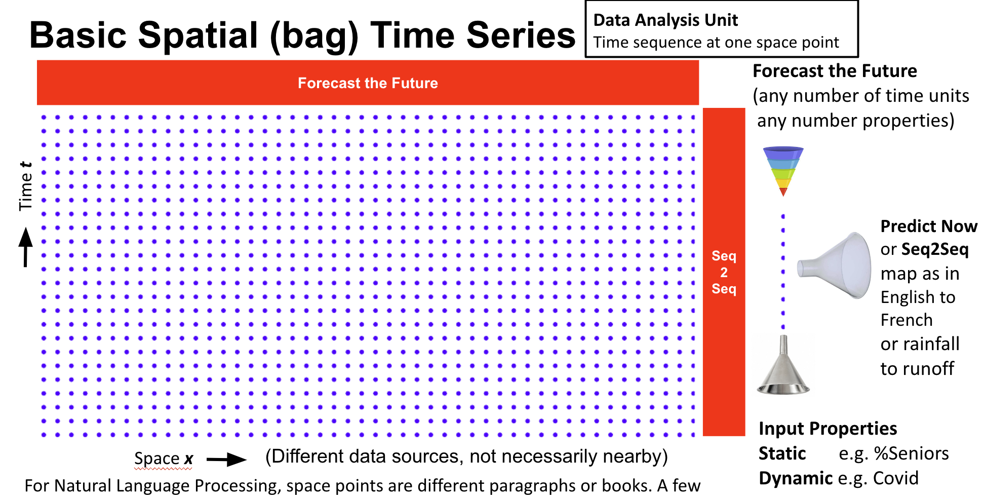
Figure 1: Spatio-temporal series layout.

I-B Rainfall-Runoff Problem

Rainfall-runoff modeling, a key challenge in hydrology, aims to model the physical process by which water on land surface (precipitation or snowmelt) moves to streams [6]. As part of the hydrologic cycle, precipitation on land either evaporates, transpires, infiltrates to recharge groundwater, or becomes surface runoff entering a catchment [6]. A catchment, or watershed, is an area where all precipitation collects and drains into a common outlet, such as a river, lake, or reservoir [6]. Surface runoff contributes to streamflow, which is defined as the volumetric discharge that takes place in a stream or channel. Runoff $RO$ can be estimated with Equation. 1, where $Q$ is streamflow, and $GW_{out}$ is ground-water outflow. Stream outflow $Q$ can be estimated with Equation. 2, where $P$ is precipitation, $GW_{in}$ is ground-water inflow, $ET$ is evapotranspiration, $\Delta S$ is the change in liquid and solid forms of storage. Eventually, this streamflow and ground water outflow reaches the ocean, where it evaporates, condenses into clouds, and returns as rainfall on land, completing the hydrologic cycle [6].

$$RO=Q+GW_{out}\vspace{-4mm}$$ (1)

$$Q=P+GW_{in}-GW_{out}-ET-\Delta S$$ (2)

Rainfall, like many natural phenomena, is periodic, with daily patterns that follow consistent seasonal cycles. While streamflow result from precipitation, it is also influenced by static environmental factors such as soil type, land cover, slope, etc. Based on this, we hypothesize that daily streamflow in a catchment can be predicted using a combination of daily meteorological forcing data, and the spatially and temporally distributed hydrologic, climatologic, geologic, pedologic, and land-use data [6]. Additionally, a neural network can learn the seasonal patterns of these hydrological processes to produce accurate forecasts.

I-C Related Work

Traditional rainfall-runoff modeling has typically focused on individual catchments. The first documented model, introduced in 1851, used linear regression to predict discharge from precipitation intensity and runoff [7]. Since then, scientific advancements have led to more sophisticated models based on mathematical formulas and physical laws. The advent of computers brought digital hydrological models. At a time when computers are expensive, slow, and low in memory, the Stanford Watershed Model [8] was proposed. It was seen as one of the first and most successful digital computer models [9]. As computers become more powerful, distributed models [10, 11] emerged, allowing for hydrological models to closely couple to geographical information systems for the input data [9]. Taking advantage of the number of parameters offered, these physical-based distributed models perform exceptionally well. However, the high computational cost to calibrate these parameters, and the limited availability of data hinder their use in large-scale forecasting applications [12].

Groundbreaking advancements in deep learning models and the publication of structured large-sample Hydrology dataset have overcome this limitation, enabling the study of nation or global scale rainfall-runoff modeling [13, 14]. In the 1990s, Artificial Neural Network (ANN) based rainfall-runoff model was proposed [15, 16, 17]. Although scientists were initially hesitant to embrace this novel “black box” approach due to the lack of extensive studies, deep learning based Hydrology models proved successful [17]. Its exceptional capability in simulating complex non-linear systems is particularly advantageous for Hydrology modeling. In 2018, the focus of the field shifted towards Long Short-Term Memory (LSTM) based models, which excelled in learning sequential dependencies within time series data [13] [18]. These models have shown great success in large-scale hydrological time series predictions. Further studies explored the interpretability of such LSTM models within physics context [19]. Since then, an open source library for the LSTM based rainfall-runoff model was published [20].

II Data And Methods

II-A Datasets selection

Hydrology data comprises of both time series and static exogenous features. It falls within the scope of spatio-temporal series since all time series properties (eg. mean temperature, streamflow) are collected and organized by catchment. Hydrology data is collected by gauges, which are stations that collect measurements at each catchment. Static attributes for each catchment refers to environmental conditions (eg. dominant land cover, soil aridity), as well as spatial extent and locations (eg. coordinates).

Recent deep learning studies on Hydrology have been driven by the advent of CAMELS (Catchment Attributes and Meteorology for Large-sample Studies) datasets, which established a standard for organizing big Hydrology data at different nations across the globe. The first CAMELS dataset [21], initially proposed with 671 catchments in the U.S., benchmarked the types of static and time series properties necessary for large sample hydrology datasets containing hundreds of catchments or more. The high dimensionality of static data along with the 20-year duration of daily time series data made it suitable for nation-scale Hydrology modeling using neural network models. Since then, CAMELS-standard datasets have been published for countries including the United Kingdom [22], Chile [23], Australia [24], Brazil [25], Switzerland [26], Sweden [27], France [28], etc.

II-B Three-Nation Combined CAMELS Data

Similarities shared by CAMELS-standard national datasets allow for the combination of national datasets into a large global dataset, which can be used for global-scale training. In this study, the experimental dataset was produced by combining CAMELS data from three nations: the United States[21], United Kingdom[22], and Chile. These datasets were selected as they provide the earliest available CAMELS-structured data during the data preprocessing phase of this study. We select static features and time series targets that are shared across the three datasets prior to combination.

TABLE I: Three-Nation Combined CAMELS Data Source

	CAMELS-US	CAMELS-GB	CAMELS-CL
Forcing a	Maurer [29]	CEH-GEAR [30]	CR2MET [31]
		CHESS-met [32]
Streamflow	USGS [33]	NRFA [34]	CR2 [35]
a Time series targets such as precipitation and temperature.

Although CAMELS-US, CAMELS-GB, CAMELS-CL follow the same standards, the exact choice of static attributes they include vary slightly, prohibiting simple concatenation of data. For instance, the “Land Cover” section of CAMELS-US only contains “% cover of forest” data for each catchment, while that section of CAMELS-GB contains the percent cover of all plantation types like woodland, crops, shrublands, etc. Without further details on the data measurement process for these properties, arithmetic manipulations to forge “percent cover of forest” for the CAMELS-GB dataset from the given “percent cover of woodland, crops, shrublands, etc” cannot be performed. To address this issue, the three-nation combined CAMELS dataset used in this study only contains static properties shared across the US, GB, and CL datasets. The processed dataset includes 1858 catchments, 3 dynamic, and 29 static variables.

II-C CAMELS Preprocessing

For dynamic variables, we selected the common interval of 7,031 days, spanning from October 2, 1989, to December 31, 2008. The start date of a water year, as defined by the U.S. Geological Survey, is October 1st [6]. To account for time differences between the nations, we shifted the training data by one day, beginning on October 2nd. An analysis of NaNs in data revealed no NaN values in time series data, yet some exists in the static features. Since missing data constitutes only a small percentage of total static data and occurs miscellaneously, it is filled with the mean value of that attribute from all catchments. Categorical variables are only present in the form of months from January to December. We encode them with ordinal encoding between 0 and 1 to preserve the natural order of months.

II-D Caravan

Published in 2023, the Caravan dataset [36], consists of seven preprocessed CAMELS-standard national datasets that contain identical static exogenous features and time series properties. Caravan aggregates data from 6,830 catchments across 16 nations spanning four continents, making it ideal for global rainfall-runoff modeling with large-scale hydrological data.

TABLE II: Caravan Sub-datasets

Sub-dataset	Catchments
CAMELS (US) [21]	482
CAMELS-AUS [24]	150
CAMELS-BR [25]	376
CAMELS-CL [23]	314
CAMELS-GB [22]	408
HYSETS (North America) [37]	4621
LamaH-CE [38]	479

The Caravan dataset is not constructed by identifying common static and time series properties shared by previously published versions of each sub-dataset. Instead, it is derived from data sources that differ significantly from those used in the original CAMELS datasets for various nations. While the catchments included in the Caravan sub-datasets are the same as those in the original versions, the actual data is sourced from global hydrological sources rather than the local sources used in the original publications. This shift to global sources enables the collection of more standardized and abundant data, making it suitable for global-scale comparative hydrological studies—one of the key motivations behind the creation of Caravan. However, it is important to note that data from global sources may vary slightly from local sources, which are often more precise. For example, in the CAMELS-US sub-dataset within Caravan, all forcing data is sourced from ERA5-Land [39], streamflow data from GSIM [40] [41], and static properties from HydroATLAS [42]. In contrast, the original CAMELS-US [21] dataset included static and time series data from three sources: NLDAS [43], Maurer [29], and DayMet [44], with streamflow data from USGS [33]. After comparison, only the streamflow data remains consistent between CAMELS-US in the original publication and in Caravan. The correlation coefficient for precipitation time series data between different data sources is presented in III. Nevertheless, the Caravan paper [36] addresses this concern, noting that the correlations between Caravan and each of the three CAMELS-US data products are not consistently lower than the correlations within the individual CAMELS-US data products.

TABLE III: CAMELS-US Caravan Comparison

	Maurer	Daymet	NLDAS
Caravan	0.71532	0.60720	0.75441

III Methods

III-A Long Short-Term Memory

The Long Short-Term Memory (LSTM) network [45] is a specialized variant of a Recurrent Neural Network (RNN) designed to address the vanishing gradient problem through its unique memory cell structure. In an LSTM block (as shown in the figure below), the cell state (denoted by $C$) serves as long-term memory. Minimal weight updates to the cell state during backpropagation effectively mitigate the vanishing gradient problem, making LSTM particularly well-suited for time series tasks involving long sequences of data. Additionally, the hidden state (denoted by $h$) serves as short-term memory. Weights (denoted by $W$) and biases (denoted by $b$) are applied to the input and passed through sigmoid and tanh activation functions. The output from the hidden state is then used to update the cell state, while the updated cell state, in turn, informs the hidden state during the final stage of computation within the LSTM block.

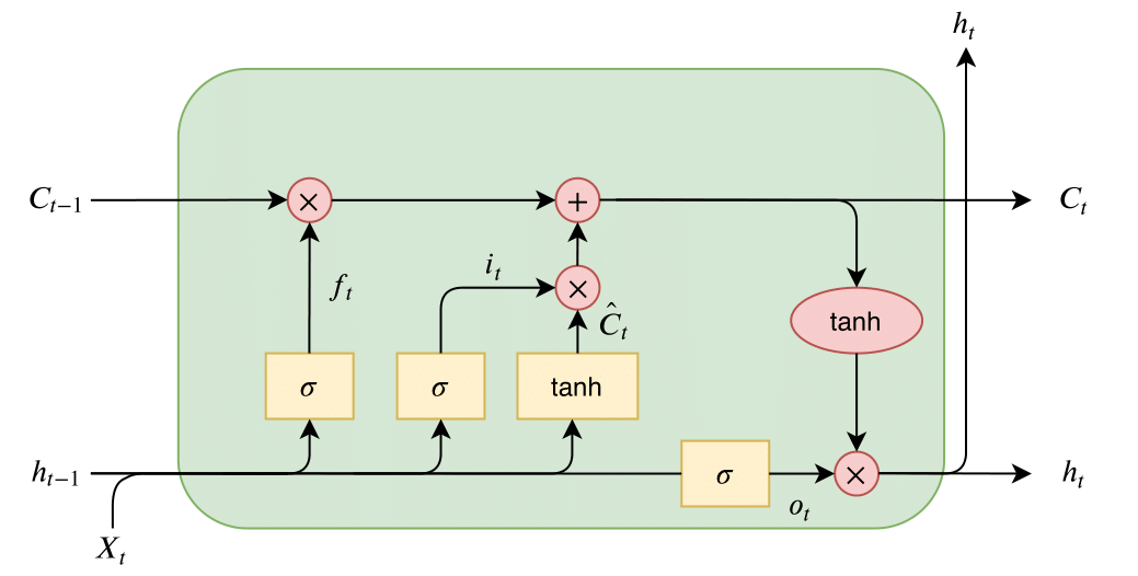
Figure 2: LSTM network.

Forget gate. Initially, the input $X_{t}$ is combined with the previous hidden state $h_{t-1}$ through the forget gate, which determines how much of the long-term memory is preserved. As shown in Equation 3, $f_{t}$ represents the forget gate value, $W_{f}$ denotes the input weights for the forget gate, $U_{f}$ refers to the recurrent weights for the forget gate, and $b_{f}$ is the bias term for the forget gate.

Input gate. Next, the input $X_{t}$ passes through the input gate, which determines the specific information to be incorporated into the long-term memory. As shown in Equation 4, $i_{t}$ represents the input gate value, $\hat{C}_{t}$ denotes the temporary cell state value, $W_{i}$ represents the input weights for the input gate, $U_{i}$ refers to the recurrent weights for the input gate, and $b_{i}$ is the bias term for the input gate.

Output gate. Lastly, the input $X_{t}$ passes through the output gate, which updates the short-term memory. As shown in Equation 6, $O_{t}$ represents the output gate value, $W_{o}$ is the input weights for the output gate, $U_{o}$ is the recurrent weights for the output gate, and $b_{o}$ is the bias term for the output gate.

Cell state and hidden state. The outputs from the forget gate, input gate, and output gate are applied to the previous cell state and hidden state to calculate the new ”long-term” and ”short-term” memory values. As shown in Equations 7 and 8, $C_{t}$ represents the updated cell state (long-term memory), and $h_{t}$ represents the updated hidden state (short-term memory).

$$f_{t}=sigmoid(W_{f}\times x_{t}+U_{f}\times h_{t-1}+b_{f})\vspace{-5mm}$$ (3)

$$i_{t}=sigmoid(W_{i}\times x_{t}+U_{i}\times h_{t-1}+b_{i})\vspace{-5mm}$$ (4)

$$\hat{C}_{t}=tanh(W_{i}\times x_{t}+U_{i}\times h_{t-1}+b_{i})\vspace{-5mm}$$ (5)

$$O_{t}=sigmoid(W_{o}\times x_{t}+U_{o}\times h_{t-1}+b_{o})\vspace{-5mm}$$ (6)

$$C_{t}=C_{t-1}\times f_{t}+i_{t}\times\hat{C}_{t}\vspace{-5mm}$$ (7)

$$h_{t}=O_{t}\times tanh(C_{t})$$ (8)

III-B Model Setup

The LSTM model used in this study is implemented using the Tensorflow framework, which allows for customization of layer parameters. The baseline model architecture is shown in Fig. 3. Detailed activation function setup is shown in Tab. IV. To prevent overfitting, a dropout rate of 20% is applied to the layers.

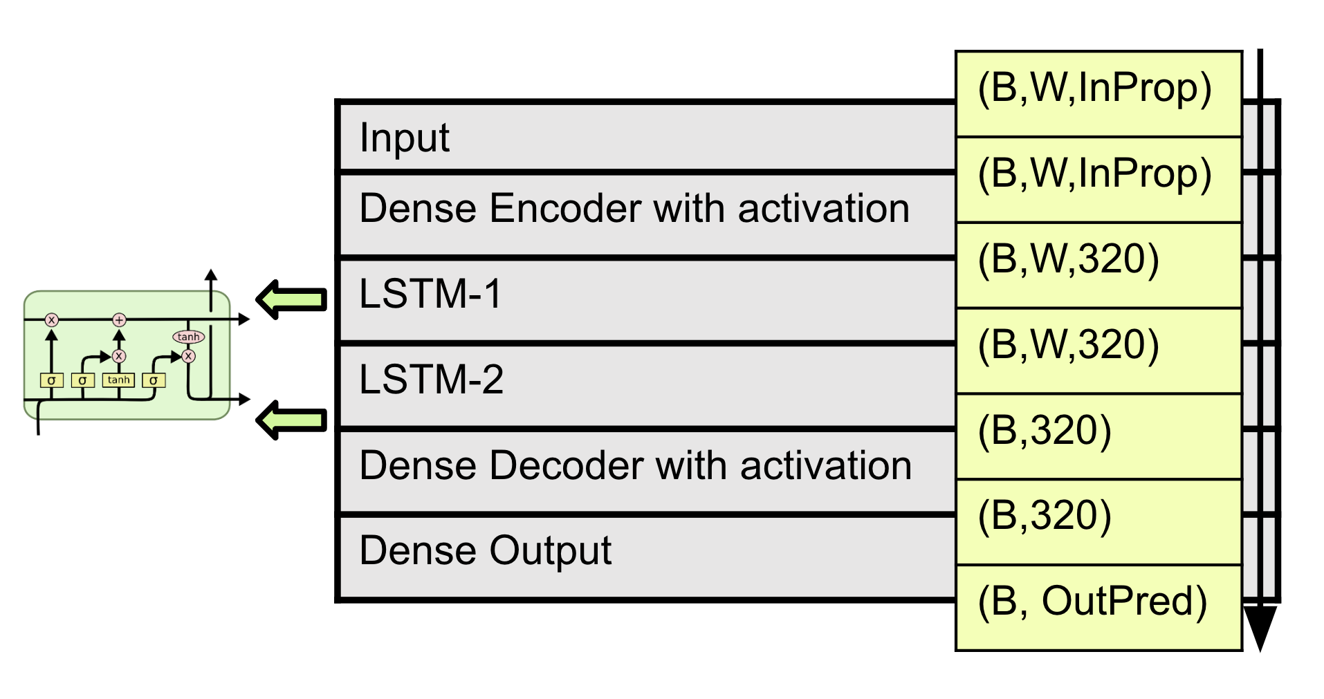
Figure 3: CAMELS-US model architecture and layer size.

TABLE IV: Model Activation Setup

Dense Encoder Activation	SELU
LSTM Recurrent Activation	Sigmoid
LSTM Layer Activation	SELU
Dense Decoder Activation	SELU

III-C Model Training and Evaluation

Inputs to the model can be classified into known inputs and observed inputs [5]. Known inputs refer to features that are known in both the past and future. In this hydrology study, static known inputs are the exogenous features such as climatic signatures, hydrologic signatures, and catchment topography. Additionally, time series known inputs exist in the form of seasonal patterns hidden in all time series features. Observed inputs are features known only for the past time periods but unknown in the future. In hydrology, those features include precipitation, temperature, and streamflow. Model output, known as targets, are the time-dependent predicted properties. In this study, predicted targets are precipitation, temperature, and streamflow.

The input data is divided into batches with a sequence length of 21 days, selected after testing various other lengths, including 7, 14, and 365 days. The 3-week sequence length was chosen to effectively capture subtle hydrological patterns. The total number of batches processed during one epoch is calculated using Equation 9, while the batch size is determined by Equation 10. In these equations, $Day_{total}$ represents the total duration of the input data in days, $l_{seq}$ denotes the sequence length, $\#Gauges$ refers to the total number of gauges in the input data, and $\#Input\ properties$ indicates the total number of input features, including both static and time series properties.

$$\#batch/epoch=Day_{total}-l_{seq}+1\vspace{-6mm}$$ (9)

$$S_{batch}=l_{seq}\times\#Gauges\times\#Input\ properties$$ (10)

Symbolic Window. A key challenge encountered during LSTM model training was the space complexity associated with handling the training data. Under the previously mentioned batch size configuration, storing all batches prior to training requires RAM space of $O(S_{batch}\times\#batch/epoch)$. To address this issue, we leverage a symbolic window to dynamically generate batches during each epoch of training. Instead of storing the entire training set, including all batches, before training, we only store the original input data with a space complexity of $O(Day_{total}\times\#Gauges\times\#Input\ properties)$. During each epoch, we track the start index $i$ for the current batch and extract the corresponding data for the batch from the input data using $Data[day_{i}:day_{i+l_{seq}}]$. This batch is then trained, and the index $i$ is incremented before proceeding to extract the next batch. This process is repeated $\#batch/epoch$ times to complete a full epoch of training. Note: This technique is environment-dependent and may not be applicable to all frameworks.

Spatial and Temporal Encodings. Like many fields of science, hydrology time series data exhibit strong seasonal patterns. It can reasonably be assumed that, at a specific gauge location, the precipitation and streamflow in October of one year will be similar to those recorded in October of the previous year. Furthermore, research has identified the approximate water residence times in various reservoirs, such as rivers, lakes, soil, and the atmosphere [46]. To effectively capture these known dependencies within the time series properties, spatial and temporal encodings are incorporated into the model during training.

1. Linear Space: a linear function with length equaling total number of catchments in input data.

2. Linear Time: a linear function with length equaling total number of days in input time series.

3. Annual Fourier Time: a basic sine and cosine function with period equaling one year.

4. Extra Fourier Time: basic sine and cosine functions with period equaling 8, 16, 32, 64, 128 days.

5. Legendre Time: Legendre functions of degree 2, 3, and 4 with range equaling total number of days in input time series.

Spatial Validation. We employ location-based rather than temporal-based validation as the catchments in the CAMELS and Caravan datasets are uncorrelated. The training and validation datasets are randomly selected on an 8:2 ratio by location, given the extensive number of catchments included in the datasets used in this study. For example, out of the 671 catchments included in CAMELS-US dataset, 537 catchments are used for training and 134 catchments are used for validation.

NNSE. Model fit is quantified using normalized Nash-Sutcliffe Efficiency (NNSE) scores [47], calculated using Equation 11, where $T$ represents the total number of days, $Q_{m}^{t}$ represents the modeled discharge on day $t$, $Q_{o}^{t}$ represents the observed discharge on day $t$, and $\overline{Q}_{o}$ is the mean observed discharge over $T$ days. NNSE values range from 0 (poor performance) to 1 (perfect fit), with a score of 0.5 indicating that the model’s predictions are equivalent to the time-averaged mean of the observations. In this study, the NNSE value is calculated for each gauge over time $T$, and the average NNSE across all gauges in the input data is reported.

$$NNSE=\frac{\Sigma_{t=1}^{T}(Q_{m}^{t}-\overline{Q}_{o})^{2}}{\Sigma_{t=1}^{t}(Q_{o}^{t}-Q_{m}^{t})^{2}+(Q_{o}^{t}-\overline{Q}_{o})^{2}}\vspace{4mm}$$ (11)

IV LSTM Benchmark Runs

IV-A Experiment Setup

All experiments are conducted using the model architecture shown in Fig. 3 and the activation functions listed in Table IV. The benchmark runs utilize Linear Space, Linear Time, and Annual Fourier Time encodings. Streamflow time series data is not trained but predicted as target.

IV-B Three-Nation Combined Benchmark Run

This run evaluates model performance on the combined CAMELS dataset from three nations: the US, UK, and Chile. The input data include static properties that are common across all three regions, whereas predicted targets consist of precipitation, mean temperature, and streamflow. Results are demonstrated in Table V.

TABLE V: CAMELS Three-Nations Combined Benchmark Run

		MSE	NNSE
	Train	0.002764	0.847
Precipitation	Val	0.003200	0.836
	Train	0.000212	0.933
Mean Temperature	Val	0.000356	0.933
	Train	0.000432	0.697
Streamflow	Val	0.000613	0.654
	Train	0.003438	-
Total	Val	0.004325	-

IV-C CAMELS Caravan US Benchmark Runs

The runs compare model performance between the original CAMELS-US dataset and the US sub-dataset within the Caravan dataset. The CAMELS-US model is trained using selected static and time series data from the original CAMELS-US dataset, while the Caravan-US model is trained using selected static and time series data from the US sub-dataset within Caravan. For both runs, we utilize the same time series features—precipitation and mean temperature—for training and predict the same targets: precipitation, mean temperature, and streamflow. Results are presented in Table VI.

TABLE VI: CAMELS Caravan US Comparison

		CAMELS-US		Caravan US
		MSE	NNSE	MSE	NNSE
	Train	0.003508	0.820	0.002920	0.851
Precipitation	Val	0.003585	0.819	0.004307	0.801
	Train	0.000276	0.961	0.000468	0.967
Mean Temperature	Val	0.000283	0.960	0.000573	0.963
	Train	0.000287	0.806	0.000525	0.814
Streamflow	Val	0.000296	0.812	0.000955	0.703
	Train	0.004111	-	0.003982	-
Total	Val	0.004203	-	0.005987	-

IV-D Caravan PCA Runs

This experiment explores the use of Principal Component Analysis (PCA) [48] to reduce the dimensionality of static properties in the Caravan input data. The Caravan sub-datasets contain over 200 static properties, nearly seven times more than the number of static input properties used in the original CAMELS studies. While this extensive range of static properties enhances model training, it significantly increases computational demands and GPU usage. To address this, we apply PCA, a widely adopted dimensionality reduction technique, to reduce the number of static input features to a level comparable with that in the CAMELS studies. In this experiment, we set the explained variance threshold to 90%, resulting in the reduction of static input features to approximately 30.

The first part of the experiment assesses the effect of PCA on model trained on US sub-dataset within the Caravan dataset, representing a small-scale input. The second part of the experiment examines the effect of PCA on model trained on North America regional data (HYSETS) [37] within the Caravan dataset, representing a large-scale input.

Results, shown in Table VII and Table VIII, indicate that the models trained with static properties obtained from PCA perform comparably to the models trained with original static properties, demonstrating that the reduction in input static dimensionality does not significantly compromise model accuracy. These findings validate PCA as an effective approach for train hydrology time series models with high static dimensionality.

TABLE VII: Caravan US PCA Experiment

		Original Static		PCA Static
		MSE	NNSE	MSE	NNSE
	Train	0.002920	0.851	0.002994	0.848
Precipitation	Val	0.004307	0.801	0.004264	0.800
	Train	0.000468	0.967	0.000468	0.967
Mean Temperature	Val	0.000573	0.963	0.000548	0.965
	Train	0.000525	0.814	0.000569	0.799
Streamflow	Val	0.000955	0.703	0.000989	0.703
	Train	0.003982	-	0.004075	-
Total	Val	0.005987	-	0.005871	-

TABLE VIII: Caravan Hysets PCA Experiment

		Original Static		PCA Static
		MSE	NNSE	MSE	NNSE
	Train	0.002714	0.835	0.002809	0.830
Precipitation	Val	0.002960	0.826	0.003055	0.821
	Train	0.000372	0.968	0.000386	0.967
Mean Temperature	Val	0.000385	0.966	0.000397	0.965
	Train	0.000614	0.825	0.000699	0.813
Streamflow	Val	0.000876	0.798	0.000397	0.799
	Train	0.003470	-	0.003611	-
Total	Val	0.003897	-	0.003926	-

IV-E Caravan Global Benchmark Run

This study provides insights into the model’s applicability to large-scale global hydrology datasets. The input data is compiled by concatenating all seven Caravan sub-datasets, which encompass catchments from four continents. As shown in Table IX, accuracy decreases slightly compared to small-scale, individual nation fits (Table VI), yet overall model performance remains relatively high, demonstrating its robustness on global datasets.

TABLE IX: Caravan Global Fit

		MSE	NNSE
	Train	0.003115	0.809
Precipitation	Val	0.003223	0.808
	Train	0.000357	0.953
Mean Temperature	Val	0.000357	0.952
	Train	0.000675	0.781
Streamflow	Val	0.000740	0.768
	Train	0.003965	-
Total	Val	0.004133	-
*Model trained with PCA static features.

V Static Properties and Spatial Temporal Encodings Experiment

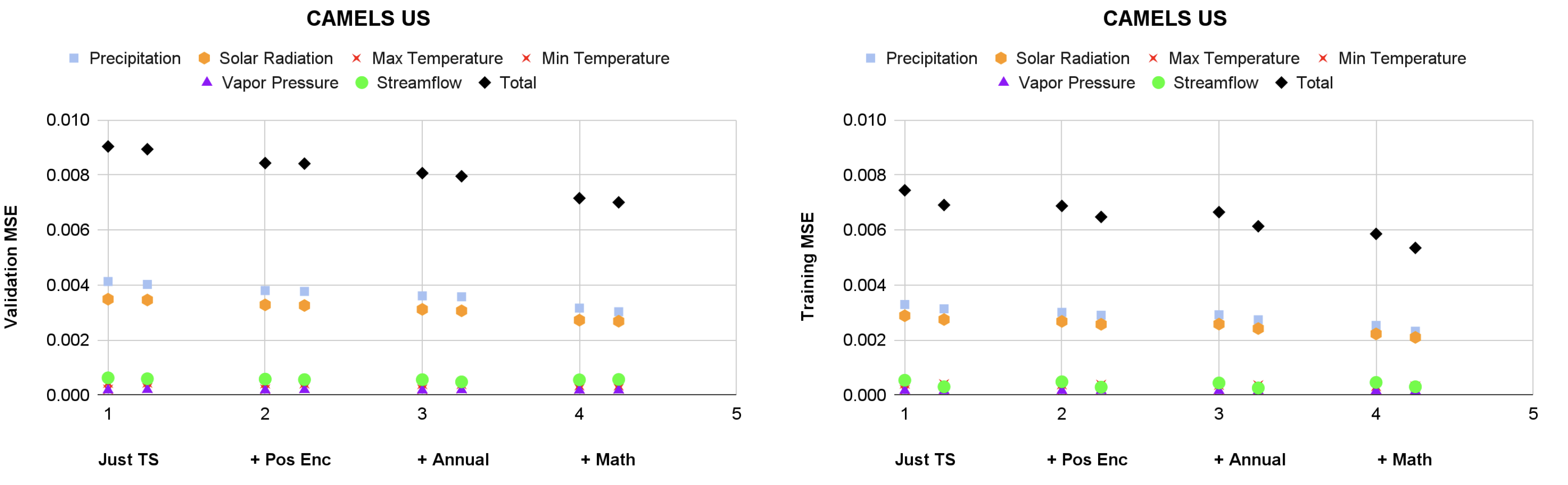
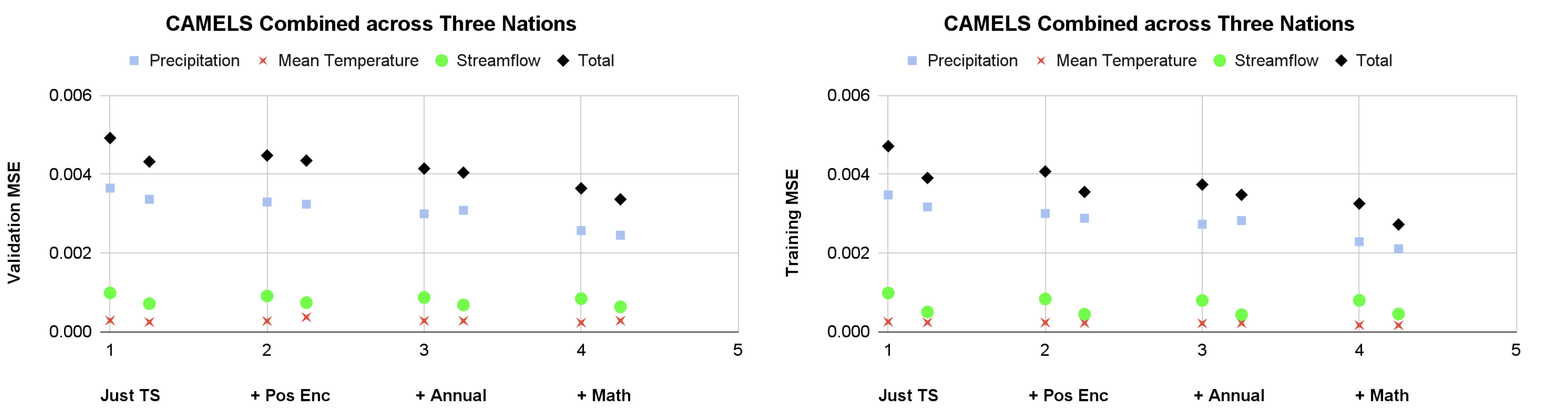
Figure 4: CAMELS US experiment (MSE loss). Each run configuration is utilized in 2 runs (left: static features not trained, right: static features trained).

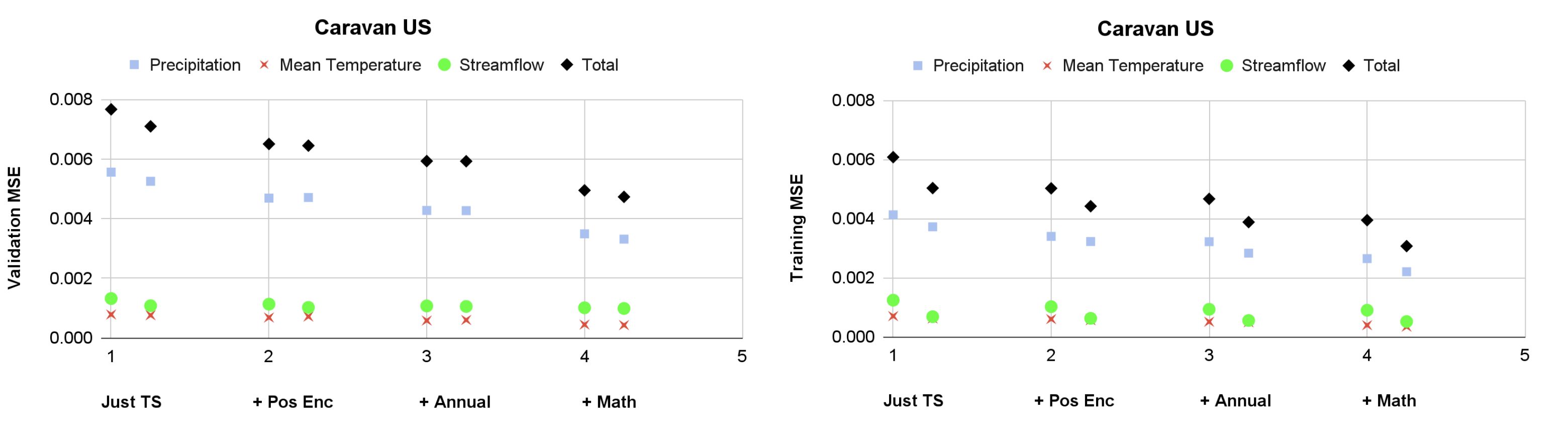
Figure 5: CAMELS three-nations combined experiment (MSE loss). Each run configuration is utilized in 2 runs (left: static features not trained, right: static features trained).

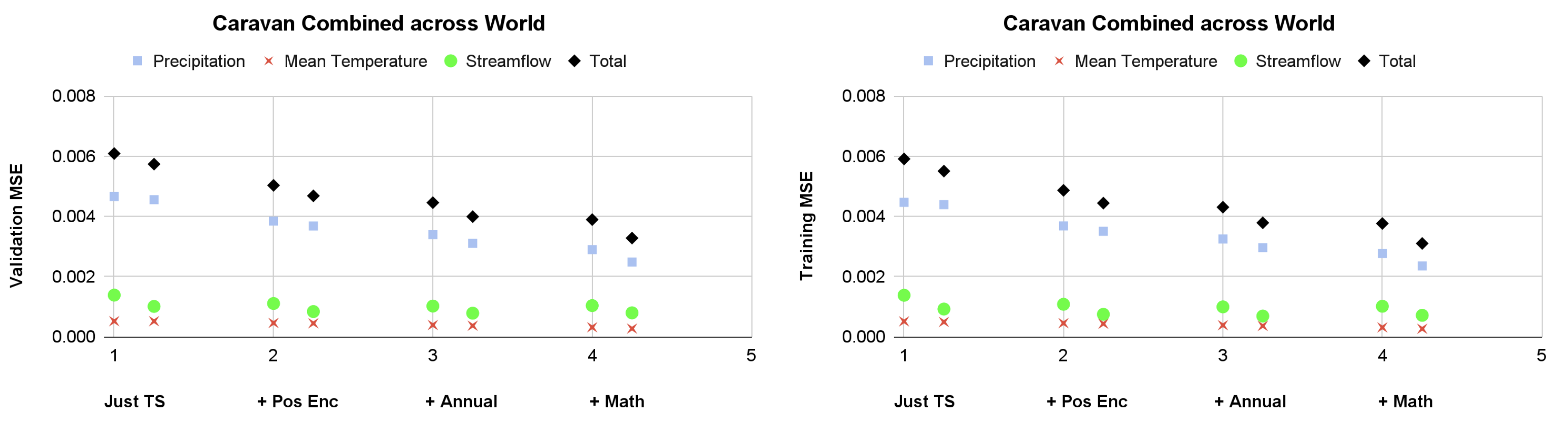
Figure 6: Caravan US experiment (MSE loss). Each run configuration is utilized in 2 runs (left: static features not trained, right: static features trained).

Figure 7: Caravan combined experiment (MSE loss). Each run configuration is utilized in 2 runs (left: static features not trained, right: static features trained).

V-A Experiment Setup

This set of experiments examines the influence of static properties and spatial-temporal encodings on rainfall-runoff modeling accuracy, demonstrated through eight run configurations on four datasets. The first experiment uses the original CAMELS-US dataset [21], representing a traditional, locally-sourced small-scale dataset. Results are presented in Fig. 7. The second experiment utilizes the Three-Nation Combined CAMELS dataset [21, 22, 23], representing a locally-sourced mid-scale dataset. Results are shown in Fig. 7. The third experiment is conducted on the US sub-dataset of the Caravan dataset [36], representing a globally-sourced small-scale dataset. Results are shown in Fig. 7. The fourth experiment uses the full Caravan concatenated dataset [36], representing a globally-sourced large-scale dataset. Results are shown in Fig. 7. All four spatial-temporal encoding configurations tested are presented in Table X. For each configuration, we conduct runs with and without static features as input to highlight the impact of static features. The model architecture remained consistent across all runs.

TABLE X: Static Properties and Encodings Experiment Configurations

	Config 1	Config 2	Config 3	Config 4
Time Series Input	✓	✓	✓	✓
Linear Space		✓	✓	✓
Linear Time		✓	✓	✓
Annual Fourier Time			✓	✓
Extra Fourier Time				✓
Legendre Time				✓

V-B Experiment Findings

Results suggest that while the addition of static features in training has a marginal effect, the LSTM network generally benefits from their inclusion. This is demonstrated by the slightly lower training and validation losses in the runs conducted with static input features for each encoding configuration, as shown in Fig. 7, Fig. 7, Fig. 7, and Fig. 7. Furthermore, the figures indicate that static input features have a greater impact on large-scale datasets compared to small-scale ones, and they appear to be more beneficial for models trained on the Caravan dataset than those trained on the CAMELS datasets. We hypothesize that this is due to the greater number of static properties used in the Caravan runs—approximately five times more than in the CAMELS runs—and that larger datasets, covering a greater number of catchments, introduce more complexity.

This study further demonstrates that spatial and temporal encoding are crucial for effectively training time series data that follow seasonal patterns. The incorporation of linear spatial-temporal encoding, as evidenced by the drop in loss from run configuration 1 to run configuration 2 in the plots, captures both the spatial relationships of catchments and the time dependence of the data. The inclusion of annual Fourier temporal encoding, shown by the drop in loss from run configuration 2 to run configuration 3, captures the yearly seasonality of hydrological data. The addition of extra Fourier and Legendre temporal encoding, indicated by the drop in loss from run configuration 3 to run configuration 4, captures both known and unknown hydrological patterns of varying lengths, thereby enhancing model performance.

In hydrology, it is reasonable to assume that interrelated time series targets are highly dependent on static properties, such as land characteristics at individual gauges. Additionally, the water cycle is governed by processes with both known and unknown periodicities, ranging from atmospheric to micro scales. However, deep learning-based time series studies often overlook the significance of these characteristics, as they are typically application-specific. Notably, recent studies tend to focus on developing state-of-the-art time series forecasting models that rely solely on raw time series data. While these foundational models allow for broad applicability across various fields, they may compromise prediction accuracy in specialized downstream applications if static features or known patterns are not incorporated into the training process.

VI Comparison with Foundation Models

Recent studies in time series analysis have focused on a foundation model approach, inspired by the success of large language models [49]. Since 2022, there has been a spike in publications on pre-trained time series foundation models, with the majority built on Transformers [50] and multi-layer perceptrons (MLPs) [51] architectures. Some models support the use of static exogenous variables as input [52, 53], while others only accept time series input [54].

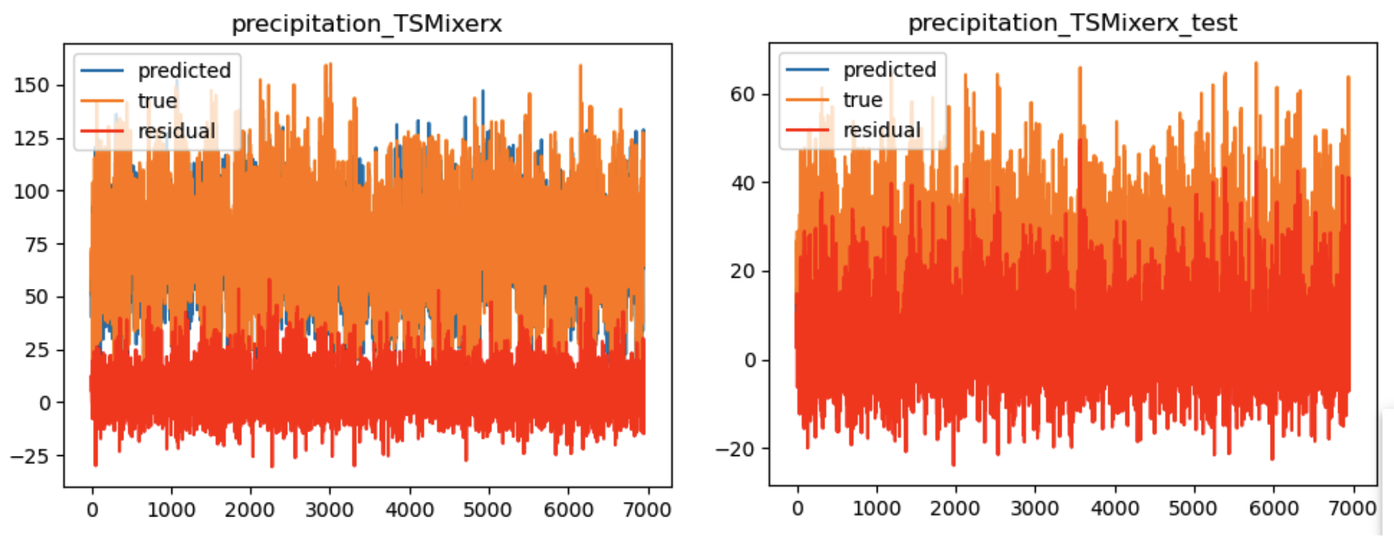
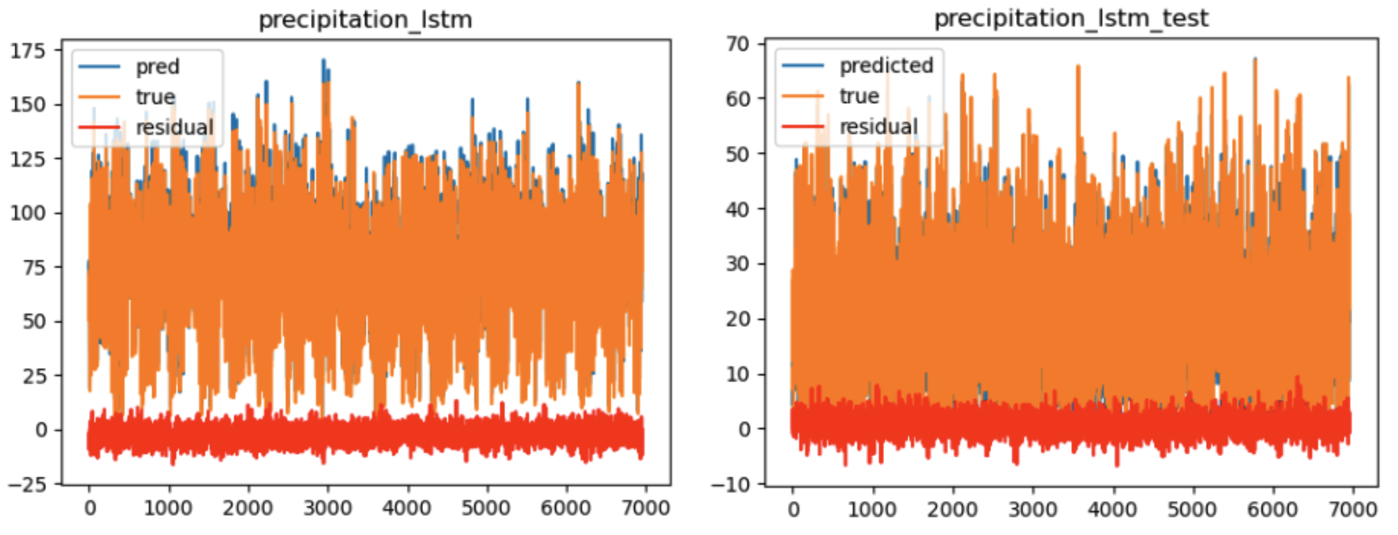
Figure 8: TSMixer precipitation fit (left: training set, right: validation set).

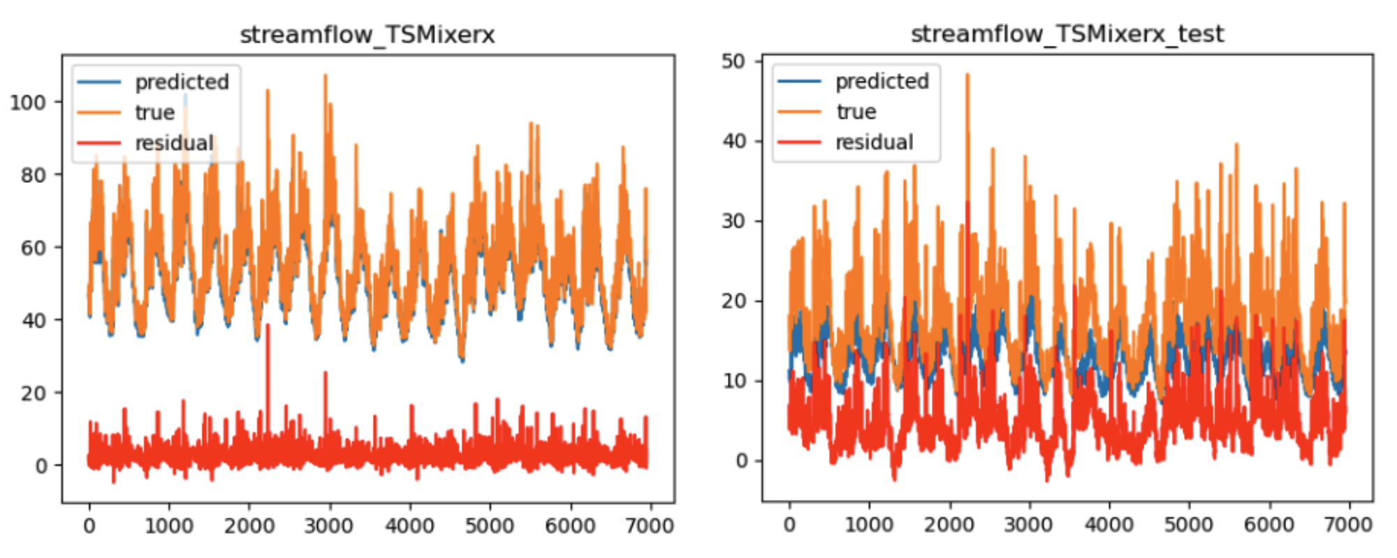
Figure 9: LSTM precipitation fit (left: training set, right: validation set).

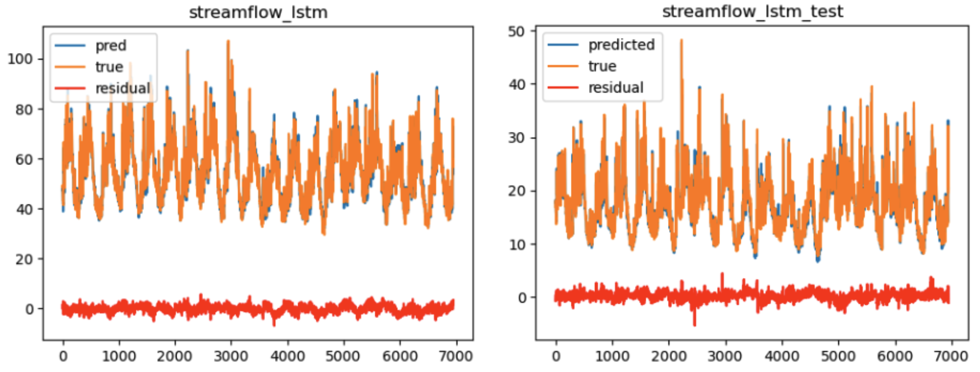
Figure 10: TSMixer streamflow fit (left: training set, right: validation set).

Figure 11: LSTM streamflow fit (left: training set, right: validation set).

In this experiment, we present a performance comparison between our LSTM-based rainfall-runoff model and the TSMixer foundation model [52] on CAMELS-US [21] data. We leverage the Nixtla Neuralforecast framework [55] to train the TSMixerx model, a variant of the TSMixer model that allows static exogenous features along with multivariate time series as input. The results, shown in Fig. 11, Fig. 11, Fig. 11, and Fig. 11, demonstrate that the LSTM model outperforms the TSMixerx model. In future work, we will expand this by looking at other time series models and a new Foundation model MultiFoundationPattern discussed for earthquakes[56].

VII Conclusion and Future Work

Often, one thinks about deep learning models discovering hidden variables that control observables that one wishes to predict. In this paper, we explored CAMELS and Caravan, which together offer large datasets covering many (about 8000) spatial locations and a long time period (around 30 years). Further, there are multiple (6 in CAMELS and 39 in Caravan) observed dynamic streams and up to 209 static (exogenous) parameters for each location. Some of these exogenous and observed data would be natural inputs into a physics model for the catchments. A priori, it is not obvious which exogenous or even endogenous data should be used as they could implied by the large datasets used in the training and implicitly learned by the training. However, most likely, it is a mixed situation where the combination of observed and exogenous data will give the best results, with the exogenous data declining in importance as the observed dataset grows in size. We clearly show in this paper with the CAMELS and Caravan data that using exogenous data makes significant improvements in the model fits where both static physical quantities and dynamical mathematical functions have value as exogenous information. In future papers, we hope to understand the trade-off better as it varies in the nature and size of exogenous data. We also will present further study of different deep learning models using the compilation of hundreds of papers and around 100 models in [57, 58, 59, 60, 61]. We aim to study a range of time series problems to build a taxonomy so that benchmark sets can be built covering the essentially different cases [62]. Another interesting feature of science time series is that they naturally vary in magnitude by large factors, and this seems not to be very consistent with neural network activation functions at fixed values independent of the stream. We will present a study of new activation functions in the LSTM using a PRELU-like (Parametric Rectified Linear Unit, or PReLU) structure, which naturally deals with magnitude changes in stream values.

References

- [1] CDC, “National Center for Health Statistics — cdc.gov,” https://www.cdc.gov/nchs/index.html, [Accessed 04-10-2024].
- [2] “Behavioral Risk Factor Surveillance System — cdc.gov,” https://www.cdc.gov/brfss/index.html, [Accessed 04-10-2024].
- [3] G. C. Fox, G. von Laszewski, F. Wang, and S. Pyne, “Aicov: An integrative deep learning framework for covid-19 forecasting with population covariates,” Journal of Data Science, vol. 19, no. 2, pp. 293–313, 2021.
- [4] “Earthquake hazards program of united states geological survey,” https://earthquake.usgs.gov/earthquakes/search/, [Accessed 04-10-2024].
- [5] G. C. Fox, J. B. Rundle, A. Donnellan, and B. Feng, “Earthquake nowcasting with deep learning,” GeoHazards, vol. 3, no. 2, pp. 199–226, 2022. [Online]. Available: https://www.mdpi.com/2624-795X/3/2/11
- [6] S. L. Dingman, Physical hydrology. Waveland press, 2015.
- [7] M. T. J., “On the use of self-registering rain and flood gauges in making observations of the relations of rainfall and flood discharges in a given catchment,” Proceedings of the Institution of Civil Engineers of Ireland, vol. 4, pp. 19–31, 1851. [Online]. Available: https://cir.nii.ac.jp/crid/1573105975719082240
- [8] N. H. Crawford, Digital simulation in hydrology : Stanford watershed model IV / by N.H. Crawford and Ray K. Linsley., ser. Stanford University Department of Civil Engineering Technical report ;, . Linsley, Ray K. (Ray Keyes), Ed. Stanford University. Dept of Civil Engineering, 1966.
- [9] K. J. Beven, Ebook Central - Academic Complete, Wiley Online Library UBCM Earth & Environmental, Wiley Online Library UBCM German Language, and Wiley Online Library UBCM All Obooks, Rainfall-runoff Modelling: The Primer. Chichester, West Sussex, Hoboken, NJ: Wiley-Blackwell, 2012.
- [10] M. Abbott, J. Bathurst, J. Cunge, P. O’Connell, and J. Rasmussen, “An introduction to the european hydrological system — systeme hydrologique europeen, “she”, 1: History and philosophy of a physically-based, distributed modelling system,” Journal of Hydrology, vol. 87, no. 1, pp. 45–59, 1986. [Online]. Available: https://www.sciencedirect.com/science/article/pii/0022169486901149
- [11] R. J. Moore and R. T. Clarke, “A distribution function approach to rainfall runoff modeling,” Water Resources Research, vol. 17, no. 5, pp. 1367–1382, 1981.
- [12] J. Sitterson, R. P. Chris Knightes, K. Wolfe, M. Muche, and B. Avant, An Overview of Rainfall-Runoff Model Types. U.S. Environmental Protection Agency, Washington, DC, 2017.
- [13] F. Kratzert, D. Klotz, C. Brenner, K. Schulz, and M. Herrnegger, “Rainfall–runoff modelling using long short-term memory (lstm) networks,” Hydrology and Earth System Sciences, vol. 22, no. 11, pp. 6005–6022, 2018. [Online]. Available: https://hess.copernicus.org/articles/22/6005/2018/
- [14] C. Shen, “A transdisciplinary review of deep learning research and its relevance for water resources scientists,” Water Resources Research, vol. 54, no. 11, pp. 8558–8593, 2018. [Online]. Available: https://agupubs.onlinelibrary.wiley.com/doi/abs/10.1029/2018WR022643
- [15] K.-l. Hsu, H. V. Gupta, and S. Sorooshian, “Artificial neural network modeling of the rainfall-runoff process,” Water Resources Research, vol. 31, no. 10, pp. 2517–2530, 1995. [Online]. Available: https://agupubs.onlinelibrary.wiley.com/doi/abs/10.1029/95WR01955
- [16] Tokar A. Sezin and Johnson Peggy A., “Rainfall-Runoff Modeling Using Artificial Neural Networks,” Journal of Hydrologic Engineering, vol. 4, no. 3, pp. 232–239, Jul. 1999, publisher: American Society of Civil Engineers. [Online]. Available: https://doi.org/10.1061/(ASCE)1084-0699(1999)4:3(232)
- [17] R. S. Govindaraju and A. R. Rao, Artificial Neural Networks in Hydrology. Springer Science & Business Media, Mar. 2013.
- [18] C. Hu, Q. Wu, H. Li, S. Jian, N. Li, and Z. Lou, “Deep learning with a long short-term memory networks approach for rainfall-runoff simulation,” Water, vol. 10, no. 11, 2018. [Online]. Available: https://www.mdpi.com/2073-4441/10/11/1543
- [19] F. Kratzert, M. Herrnegger, D. Klotz, S. Hochreiter, and G. Klambauer, NeuralHydrology – Interpreting LSTMs in Hydrology. Cham: Springer International Publishing, 2019, pp. 347–362. [Online]. Available: https://doi.org/10.1007/978-3-030-28954-6_19
- [20] F. Kratzert, M. Gauch, G. Nearing, and D. Klotz, “NeuralHydrology — A Python library for Deep Learning research in hydrology,” Journal of Open Source Software, vol. 7, no. 71, p. 4050, Mar. 2022. [Online]. Available: https://joss.theoj.org/papers/10.21105/joss.04050
- [21] N. Addor, A. J. Newman, N. Mizukami, and M. P. Clark, “The camels data set: catchment attributes and meteorology for large-sample studies,” Hydrology and Earth System Sciences, vol. 21, no. 10, pp. 5293–5313, 2017. [Online]. Available: https://hess.copernicus.org/articles/21/5293/2017/
- [22] G. Coxon, N. Addor, J. P. Bloomfield, J. Freer, M. Fry, J. Hannaford, N. J. K. Howden, R. Lane, M. Lewis, E. L. Robinson, T. Wagener, and R. Woods, “Camels-gb: hydrometeorological time series and landscape attributes for 671 catchments in great britain,” Earth System Science Data, vol. 12, no. 4, pp. 2459–2483, 2020. [Online]. Available: https://essd.copernicus.org/articles/12/2459/2020/
- [23] C. Alvarez-Garreton, P. A. Mendoza, J. P. Boisier, N. Addor, M. Galleguillos, M. Zambrano-Bigiarini, A. Lara, C. Puelma, G. Cortes, R. Garreaud, J. McPhee, and A. Ayala, “The camels-cl dataset: catchment attributes and meteorology for large sample studies – chile dataset,” Hydrology and Earth System Sciences, vol. 22, no. 11, pp. 5817–5846, 2018. [Online]. Available: https://hess.copernicus.org/articles/22/5817/2018/
- [24] K. J. A. Fowler, S. C. Acharya, N. Addor, C. Chou, and M. C. Peel, “Camels-aus: hydrometeorological time series and landscape attributes for 222 catchments in australia,” Earth System Science Data, vol. 13, no. 8, pp. 3847–3867, 2021. [Online]. Available: https://essd.copernicus.org/articles/13/3847/2021/
- [25] V. B. P. Chagas, P. L. B. Chaffe, N. Addor, F. M. Fan, A. S. Fleischmann, R. C. D. Paiva, and V. A. Siqueira, “Camels-br: hydrometeorological time series and landscape attributes for 897 catchments in brazil,” Earth System Science Data, vol. 12, no. 3, pp. 2075–2096, 2020. [Online]. Available: https://essd.copernicus.org/articles/12/2075/2020/
- [26] M. Höge, M. Kauzlaric, R. Siber, U. Schönenberger, P. Horton, J. Schwanbeck, M. G. Floriancic, D. Viviroli, S. Wilhelm, A. E. Sikorska-Senoner, N. Addor, M. Brunner, S. Pool, M. Zappa, and F. Fenicia, “Camels-ch: hydro-meteorological time series and landscape attributes for 331 catchments in hydrologic switzerland,” Earth System Science Data, vol. 15, no. 12, pp. 5755–5784, 2023. [Online]. Available: https://essd.copernicus.org/articles/15/5755/2023/
- [27] C. Teutschbein, “Camels‐se : Long‐term hydroclimatic observations (1961–2020) across 50 catchments in sweden as a resource for modelling, education, and collaboration,” Geoscience Data Journal, 2024.
- [28] O. Delaigue, P. Brigode, V. Andréassian, C. Perrin, P. Etchevers, J.-M. Soubeyroux, B. Janet, and N. Addor, “Camels-fr: A large sample hydroclimatic dataset for france to explore hydrological diversity and support model benchmarking,” in IAHS-2022 Scientific Assembly, Montpellier, France, May 2022. [Online]. Available: https://hal.inrae.fr/hal-03687235
- [29] B. Livneh, E. A. Rosenberg, C. Lin, B. Nijssen, V. Mishra, K. M. Andreadis, E. P. Maurer, and D. P. Lettenmaier, “A long-term hydrologically based dataset of land surface fluxes and states for the conterminous united states: Update and extensions,” Journal of Climate, vol. 26, no. 23, pp. 9384 – 9392, 2013. [Online]. Available: https://journals.ametsoc.org/view/journals/clim/26/23/jcli-d-12-00508.1.xml
- [30] V. D. J. Keller, M. Tanguy, I. Prosdocimi, J. A. Terry, O. Hitt, S. J. Cole, M. Fry, D. G. Morris, and H. Dixon, “Ceh-gear: 1 km resolution daily and monthly areal rainfall estimates for the uk for hydrological and other applications,” Earth System Science Data, vol. 7, no. 1, pp. 143–155, 2015. [Online]. Available: https://essd.copernicus.org/articles/7/143/2015/
- [31] J. P. Boisier, “Cr2met: A high-resolution precipitation and temperature dataset for the period 1960-2021 in continental chile.” Jan. 2023.
- [32] E. Robinson, E. Blyth, D. Clark, E. Comyn-Platt, J. Finch, and A. Rudd, “Climate hydrology and ecology research support system meteorology dataset for great britain (1961-2015) [chess-met] v1.2,” 2017. [Online]. Available: https://doi.org/10.5285/b745e7b1-626c-4ccc-ac27-56582e77b900
- [33] H. ”Lins, “”usgs hydro-climatic data network 2009 (hcdn–2009)”,” ”U.S. Geological Survey Fact Sheet 2012–3047”, 2012. [Online]. Available: ”https://pubs.usgs.gov/fs/2012/3047/”
- [34] J. Hannaford, “Development of a strategic data management system for a national hydrological database, the uk national river flow archive,” Hydroinformatics, pp. 637–644, 2004.
- [35] C. for Climate and R. Research, “Streamflow.” [Online]. Available: https://www.cr2.cl/datos-de-caudales/
- [36] F. Kratzert, G. Nearing, N. Addor, T. Erickson, M. Gauch, O. Gilon, L. Gudmundsson, A. Hassidim, D. Klotz, S. Nevo, G. Shalev, and Y. Matias, “Caravan - a global community dataset for large-sample hydrology,” Scientific Data, vol. 10, no. 1, p. 61, Jan. 2023. [Online]. Available: https://doi.org/10.1038/s41597-023-01975-w
- [37] R. Arsenault, F. Brissette, J.-L. Martel, M. Troin, G. Lévesque, J. Davidson-Chaput, M. C. Gonzalez, A. Ameli, and A. Poulin, “A comprehensive, multisource database for hydrometeorological modeling of 14,425 North American watersheds,” Scientific Data, vol. 7, no. 1, p. 243, Jul. 2020. [Online]. Available: https://doi.org/10.1038/s41597-020-00583-2
- [38] C. Klingler, K. Schulz, and M. Herrnegger, “Lamah-ce: Large-sample data for hydrology and environmental sciences for central europe,” Earth System Science Data, vol. 13, no. 9, pp. 4529–4565, 2021. [Online]. Available: https://essd.copernicus.org/articles/13/4529/2021/
- [39] J. Muñoz Sabater, E. Dutra, A. Agustí-Panareda, C. Albergel, G. Arduini, G. Balsamo, S. Boussetta, M. Choulga, S. Harrigan, H. Hersbach, B. Martens, D. G. Miralles, M. Piles, N. J. Rodríguez-Fernández, E. Zsoter, C. Buontempo, and J.-N. Thépaut, “Era5-land: a state-of-the-art global reanalysis dataset for land applications,” Earth System Science Data, vol. 13, no. 9, pp. 4349–4383, 2021. [Online]. Available: https://essd.copernicus.org/articles/13/4349/2021/
- [40] H. X. Do, L. Gudmundsson, M. Leonard, and S. Westra, “The global streamflow indices and metadata archive (gsim) – part 1: The production of a daily streamflow archive and metadata,” Earth System Science Data, vol. 10, no. 2, pp. 765–785, 2018. [Online]. Available: https://essd.copernicus.org/articles/10/765/2018/
- [41] L. Gudmundsson, H. X. Do, M. Leonard, and S. Westra, “The global streamflow indices and metadata archive (gsim) – part 2: Quality control, time-series indices and homogeneity assessment,” Earth System Science Data, vol. 10, no. 2, pp. 787–804, 2018. [Online]. Available: https://essd.copernicus.org/articles/10/787/2018/
- [42] S. Linke, B. Lehner, C. Ouellet Dallaire, J. Ariwi, G. Grill, M. Anand, P. Beames, V. Burchard-Levine, S. Maxwell, H. Moidu, F. Tan, and M. Thieme, “Global hydro-environmental sub-basin and river reach characteristics at high spatial resolution,” Scientific Data, vol. 6, no. 1, p. 283, Dec. 2019. [Online]. Available: https://doi.org/10.1038/s41597-019-0300-6
- [43] Y. Xia, K. Mitchell, M. Ek, J. Sheffield, B. Cosgrove, E. Wood, L. Luo, C. Alonge, H. Wei, J. Meng, B. Livneh, D. Lettenmaier, V. Koren, Q. Duan, K. Mo, Y. Fan, and D. Mocko, “Continental-scale water and energy flux analysis and validation for the north american land data assimilation system project phase 2 (nldas-2): 1. intercomparison and application of model products,” Journal of Geophysical Research Atmospheres, vol. 117, no. 3, 2012, copyright: Copyright 2018 Elsevier B.V., All rights reserved.
- [44] P. THORNTON, M. THORNTON, B. MAYER, N. WILHELMI, Y. WEI, R. DEVARAKONDA, and R. COOK, “Daymet: Daily surface weather data on a 1-km grid for north america, version 2,” 2014. [Online]. Available: http://daac.ornl.gov/cgi-bin/dsviewer.pl?ds_id=1219
- [45] S. Hochreiter and J. Schmidhuber, “Long short-term memory,” Neural Computation, vol. 9, no. 8, pp. 1735–1780, 1997.
- [46] M. Pidwirny, “The hydrologic cycle,” 2006. [Online]. Available: http://www.physicalgeography.net/fundamentals/8b.html
- [47] J. Nossent and W. Bauwens, “Application of a normalized Nash-Sutcliffe efficiency to improve the accuracy of the Sobol’ sensitivity analysis of a hydrological model,” in EGU General Assembly Conference Abstracts, ser. EGU General Assembly Conference Abstracts, Apr. 2012, p. 237.
- [48] S. Wold, K. Esbensen, and P. Geladi, “Principal component analysis,” Chemometrics and Intelligent Laboratory Systems, vol. 2, no. 1, pp. 37–52, 1987, proceedings of the Multivariate Statistical Workshop for Geologists and Geochemists. [Online]. Available: https://www.sciencedirect.com/science/article/pii/0169743987800849
- [49] S. Mirchandani, F. Xia, P. Florence, B. Ichter, D. Driess, M. G. Arenas, K. Rao, D. Sadigh, and A. Zeng, “Large language models as general pattern machines,” 2023. [Online]. Available: https://arxiv.org/abs/2307.04721
- [50] A. Vaswani, N. Shazeer, N. Parmar, J. Uszkoreit, L. Jones, A. N. Gomez, L. Kaiser, and I. Polosukhin, “Attention is all you need,” 2023. [Online]. Available: https://arxiv.org/abs/1706.03762
- [51] I. Tolstikhin, N. Houlsby, A. Kolesnikov, L. Beyer, X. Zhai, T. Unterthiner, J. Yung, A. Steiner, D. Keysers, J. Uszkoreit, M. Lucic, and A. Dosovitskiy, “Mlp-mixer: An all-mlp architecture for vision,” 2021. [Online]. Available: https://arxiv.org/abs/2105.01601
- [52] S.-A. Chen, C.-L. Li, N. Yoder, S. O. Arik, and T. Pfister, “Tsmixer: An all-mlp architecture for time series forecasting,” 2023. [Online]. Available: https://arxiv.org/abs/2303.06053
- [53] A. Das, W. Kong, A. Leach, S. Mathur, R. Sen, and R. Yu, “Long-term forecasting with tide: Time-series dense encoder,” 2024. [Online]. Available: https://arxiv.org/abs/2304.08424
- [54] A. F. Ansari, L. Stella, C. Turkmen, X. Zhang, P. Mercado, H. Shen, O. Shchur, S. S. Rangapuram, S. P. Arango, S. Kapoor, J. Zschiegner, D. C. Maddix, H. Wang, M. W. Mahoney, K. Torkkola, A. G. Wilson, M. Bohlke-Schneider, and Y. Wang, “Chronos: Learning the language of time series,” 2024. [Online]. Available: https://arxiv.org/abs/2403.07815
- [55] K. G. Olivares, C. Challú, F. Garza, M. M. Canseco, and A. Dubrawski, “Neuralforecast: User friendly state-of-the-art neuralforecasting models.” PyCon Salt Lake City, Utah, US 2022, 2022. [Online]. Available: https://github.com/Nixtla/neuralforecast
- [56] A. Jafari, G. Fox, J. B. Rundle, A. Donnellan, and L. G. Ludwig, “Time series foundation models and deep learning architectures for earthquake temporal and spatial nowcasting,” arXiv [cs.LG, physics.geo-ph], 22 Aug. 2024. [Online]. Available: http://arxiv.org/abs/2408.11990
- [57] “ScienceFMHub portal for science foundation model community,” http://sciencefmhub.org, 2 Nov. 2023, accessed: 2023-11-3.
- [58] “Nixtla: A future for everybody. time series research and deployment,” https://www.nixtla.io/, accessed: 2024-3-9.
- [59] ddz, “Awesome time series forecasting/prediction papers: a reading list of papers on time series forecasting/prediction (TSF) and spatio-temporal forecasting/prediction (STF),” https://github.com/ddz16/TSFpaper, accessed: 2024-5-16.
- [60] M. Jin, Q. Wen, Y. Liang, C. Zhang, S. Xue, X. Wang, J. Zhang, Y. Wang, H. Chen, X. Li, S. Pan, V. S. Tseng, Y. Zheng, L. Chen, and H. Xiong, “Large models for time series and spatio-temporal data: A survey and outlook,” arXiv [cs.LG], 16 Oct. 2023. [Online]. Available: http://arxiv.org/abs/2310.10196
- [61] Y. Liang, H. Wen, Y. Nie, Y. Jiang, M. Jin, D. Song, S. Pan, and Q. Wen, “Foundation models for time series analysis: A tutorial and survey,” arXiv [cs.LG], 21 Mar. 2024. [Online]. Available: http://arxiv.org/abs/2403.14735
- [62] X. Huang, G. C. Fox, S. Serebryakov, A. Mohan, P. Morkisz, and D. Dutta, “Benchmarking deep learning for time series: Challenges and directions,” in 2019 IEEE International Conference on Big Data (Big Data). ieeexplore.ieee.org, Dec. 2019, pp. 5679–5682. [Online]. Available: http://dx.doi.org/10.1109/BigData47090.2019.9005496