Future-Guided Learning: A Predictive Approach To Enhance Time-Series Forecasting

Abstract

Accurate time-series forecasting is essential across a multitude of scientific and industrial domains, yet deep learning models often struggle with challenges such as capturing long-term dependencies and adapting to drift in data distributions over time. We introduce Future-Guided Learning, an approach that enhances time-series event forecasting through a dynamic feedback mechanism inspired by predictive coding. Our approach involves two models: a detection model that analyzes future data to identify critical events and a forecasting model that predicts these events based on present data. When discrepancies arise between the forecasting and detection models, the forecasting model undergoes more substantial updates, effectively minimizing surprise and adapting to shifts in the data distribution by aligning its predictions with actual future outcomes. This feedback loop, drawing upon principles of predictive coding, enables the forecasting model to dynamically adjust its parameters, improving accuracy by focusing on features that remain relevant despite changes in the underlying data. We validate our method on a variety of tasks such as seizure prediction in biomedical signal analysis and forecasting in dynamical systems, achieving a 40% increase in the area under the receiver operating characteristic curve (AUC-ROC) and a 10% reduction in mean absolute error (MAE), respectively. By incorporating a predictive feedback mechanism that adapts to data distribution drift, Future-Guided Learning offers a promising avenue for advancing time-series forecasting with deep learning.

1 Introduction

Time-series forecasting is a well-researched area in statistics and machine learning, with wide applicability in financial markets, weather prediction, and biomedical signal analysis. More recently, Deep Learning has emerged as a powerful tool for learning via the parallel-processing of deep-neural-networks, and has been especially beneficial in natural language processing and computer vision.

Despite success in these domains, Deep Learning has struggled to find similar progress in long-term time-series forecasting, where the inherent stochasticicity and noise of signals leads poses a unique challenge. Unlike static data, time-series involves complex temporal dependencies; predictions must account for dynamic relationships across time. As a result, many traditional deep learning models, including recurrent neural networks (RNNs), often fall short when tasked with long-term predictions.

To tackle these challenges, we draw inspiration from Knowledege Distillation (KD). Initially proposed by [11], KD involves transferring information from a large teacher model to a smaller student model via comparison of the two models class probabilities. The goal is to enable the student network to preserve the performance of the teacher [5]. Traditional KD methods are mostly focused on transferring spatial knowledge [10], and more recently, for enabling lightweight, task/domain-specific language models [17, 33].

Time-series forecasting provides a unique opportunity to apply KD in a new way—by allowing a future-oriented teacher model to guide a past-oriented student model, enhancing the latter’s ability to make accurate long-term predictions. This temporal variance between teacher and student is at the core of our framework, Future-Guided Learning (FGL).

Importantly, FGL is rooted in the theory of Predictive Coding. This theory posits the brain as an inference machine, constantly predicting the state of the external environment and adjusting its internal models based on observed discrepancies, known as "prediction errors" [32, 8, 26, 15]. This process is inherently temporal, as it involves updating predictions over time to minimize error and refine future estimates. In its hierarchical form, predictive coding posits that neurobiological networks compute these errors across different levels of abstraction, progressively building internal models of the world [23, 27].

Despite its potential to model spatio-temporal information, predictive coding’s impact on modern deep learning has been limited [19, 9]. Prior research has explored its use as a biologically plausible alternative to gradient descent [20] and applied it in hierarchical recurrent networks for supervised and unsupervised learning tasks [31, 27]. However, integrating predictive coding with modern deep learning methods to handle the temporal dynamics and uncertainty inherent in tasks like time-series forecasting remains an open challenge.

In this work, we validate FGL across two distinct domains: biomedical signal analysis and time series forecasting. In the biomedical domain, we focus on seizure prediction using EEG data, where results show an average increase of 40% in AUCROC across patients. In the forecasting domain, we validate FGL’s benefits on dynamical systems forecasting of the Makcey Glass equation, where a 10% decrease in Mean Absolute Error (MAE) is observed. The results demonstrate that FGL not only improves forecasting accuracy, but also introduces a robust method for utilizing uncertainty across time horizons, naturally connecting itself to predictive coding theory.

2 Related Work

Other works have explored the time-domain in knowledge distillation, particularly in sequence-based tasks like speech recognition [6, 7, 35] and language modeling [12], and have excelled at transfer learning and model compression. While these approaches are useful in their domains, the uncertainty of a sequential model will vary as a function of the forecasting horizon; KD is yet to take advantage of the relationship between a model’s temporal dynamics and variance in uncertainity.

In the non-KD domain, some researchers have used a future-model to aid a past-model for unsupervised and self-supervised learning. For instance, [34] used a seizure detector as an annotator for a predictor model. On the other hand, [28] introduced a novel framework which enabled a human-action-recognition network to supervise the training of an action-anticipatory network by accounting for positional shifts.

Several attempts have also been made to modernize Predictive Coding within deep learning frameworks. For instance, [22] propose a general-approach for unsupervised representation learning by using an autoencoder to predict the future latent space, while [18] use stacked LSTM cells with layer-wise predictions for unsupervised learning. These works helped to bridge the gap between neuroscience theory and deep learning applications, however, with the fast pace of research and new methods/architectures, a more generalizeable framework-based approach is warranted.

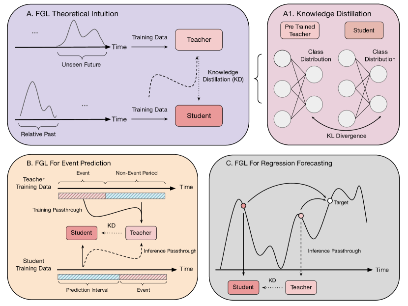
Figure 1: (A) In the FGL framework, a teacher model operates in the relative future of a student model which focuses on long-term forecasting. After the teacher is trained on its future-oriented task, during the student’s training, inference is performed on both models. The probability distributions from both the teacher and student are extracted, and a loss is computed based equation 1.(A1) Knowledge distillation involves the transfer of information via the KL divergence between class distributions. (B) In an event prediction setting, the teacher is trained on the events themselves, wheras the student is trained to predict said events. Thus, the student gains intution from the teacher at its training time. (C) In a regression forecasting scenario, the teacher and student perform short and long term forecasting respectively. Similar to event prediction, the student gains insight from the teacher during training, improving its ability to predict further into the future.

3 Methodology

Traditional KD involves distilling probabilistic class information between two models with the same representation space. We reformulate the student-teacher dynamic presented in traditional KD, namely, the teacher is now in the relative future of the student model such that there is a temporal variance in the representation space between the student and teacher models.

Our method of distillation follows that of Hinton et al. [11], in that we take the cross-entropy between the student and true data, and the Kullback-Leibler (KL) divergence of the class distributions of each model via softmaxed logits.

$$\mathcal{L}=\alpha\times\underbrace{-\sum_{i}Y_{\text{true},i}\cdot\sigma(\text{logits}_{S,i})}_{\text{Cross-Entropy Loss}}+\beta\times\underbrace{\sum_{i}\sigma(\text{logits}_{T,i}/t)\cdot\left[\log\left(\frac{\sigma(\text{logits}_{T,i}/t)}{\sigma(\text{logits}_{S,i}/t)}\right)\right]}_{\text{Time-Offset KL divergence Loss}}$$ (1)

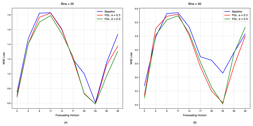
Figure 3: Mackey Glass forecasting results with (A) 25 and (B) 50 bins. Results show the mean MAE loss from 5 trials at each horizon. We experiment with two levels of $\alpha$, at 0.5 and 0.0. MAE loss is computed as the difference between the predicted bin and the true bin, where the true bin corresponds to the neuron with the highest predicted probability. A table of results is available in Appendix B.

In the above equation, $\alpha$ and $\beta$ are learnable hyperparameters that scale each component of the loss function, temperature $t$ determines how ‘soft’ the softmax function is for both teacher and student. Most importantly, the logits between both models are offset in time: the teacher $T$ logits in the numerator and the student $S$ logits in the denominator are obtained at different steps in time over a sequence. As an illustrative example, given time-series biomedical signal data (such as from an electroencephalogram, EEG) $X_{t}$ which is sampled at time $t$, the student $S$ aims to forecast whether a seizure will occur $n-steps$ into the future $t+n$, while the teacher $T$ determines whether a seizure is presently occurring at time $t$. A high-level illustration is provided in Figure 3.

The KL divergence compares the probability distributions of the student and teacher, thereby distilling the ‘uncertainty’ of the teacher model to the student; the student is encouraged by the KL loss function to learn closely-related spatial and temporal information of the teacher. Throughout the rest of this paper, $\beta$ is substituted for $1-\alpha$ such that $\alpha+\beta=1$.

The significance of the distillation loss function is the temporal offset between the student and teacher models. For any student time step $t$, the teacher network has a different temporal correlation with respect to its own underlying data distribution, allowing us to distill time-variant uncertainty from the teacher model.

4 Future-Guided Learning For Event Prediction

Seizure forecasting is an effective way to test FGL, as it is possible to detect both seizures as well as forecast them in advance. More acutely, a seizure detector model may be able to provide useful insights to a seizure forecasting model, which does not learn what a seizure is, but must be able to accurately predict them.

For the task of seizure forecasting, two main datasets are used: the Childrens Hospital Boston MIT (CHBMIT) dataset [24], as well as the American Epillepsy Society Seizure Prediction Challenge (AES) dataset [4]. Further background information and preprocessing details are available in Appendix A.1 and A.2 respectively.

4.1 CHBMIT: Patient Specific FGL

On the CHBMIT dataset, FGL was preformed by first pre-training a teacher model for seizure detection on each patient for $50$ epochs. During this process, preictal segments were concealed as their inclusion would undermine the uncertainty that we wish to extract post-hoc in the student training loop. Next, during the training of the student model over $25$ epochs, each data point is passed into both the student and teacher, and class probabilities are obtained. The loss function in Equation (1) is then used to calculate the loss of the student model. Different values of $\alpha$ correspond to different loss weightings for the student, and the best parameter is chosen for each patient with a hyperparameter sweep. Temperature is held constant at $T=4$ for the KD loss. The SGD optimizer was used with a learning rate of $5\times 10^{-4}$. Both the student and teacher models are CNNLSTMS.

4.2 AES: Patient Non-Specific FGL

In the absence of future data relative to the student’s distribution, it is still possible to train a teacher using future data that is out-of-distribution. We test this theory on the American Epilepsy Society (AES) dataset. This dataset only contains samples of preictal data without any seizures themselves. Due to the inability to match preictal periods with their corresponding seizures, we use a separate dataset to create the teacher, the UPenn and Mayo Clinic seizure dataset [14].

While the AES dataset consists of 5 dogs and 2 humans, the UPenn and Mayo Clinic dataset consists of 4 dogs and 8 human patients. Due to this mismatch, we opted to create two "universal teachers" from the latter dataset based on dog seizures and human seizures. Our universal teachers were created by combining data from a select set of patients, concatenating all their interictal data, and interspersing them between random seizures from our pool of patients such that the teacher model learns the features of many different seizures.

One restriction of using multiple data sources for our teacher was inconsistency of the data. We overcame this challenge by selecting only the $n$ most significant channels for each teacher patient via their contribution to seizure detection scores [29], and vary the number of selected channels based on the needs of each student model.

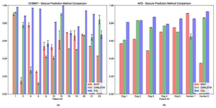
Figure 2: Seizure Prediction results on (a) CHBMIT and (b) AES datasets. Three methods are tested: an MViT, a CNN-LSTM, and FGL. All results were calculated over 3 continuous trials. The means and variance bars are reported.

4.3 Event Prediction Discussion

Our results on both the CHBMIT and AES datasets show a remarkable improvement in predictive accuracy. On the CHBMIT dataset, a 40% increase is observed on average across all patients. We find these increases are not evenly distributed; FGL leads to remarkable improvements on patients 3, 5, 10, and 20, with a less-noticeable increase on others. We posit that the variability in FGL’s predictive performance may be due to a variety of factors, including number of predicable seizures, strength of teacher model, and inherent noise in EEG signals.

Conversely, the AES dataset finds a more consistent increase across patients, leading to an average improvement of 30%. We believe this may attributed to the formulation of the teacher model. Unlike the cHBMIT dataset, which used patient-specific teacher models, FGL on AES utilized a teacher model trained from a pool of seizures, potentially stabilizing its benefits for prediction.

5 Future-Guided Learning For Regression Forecasting

Seizure prediction typically involves the analysis of EEG signals as the primary modality of data. These signals are typically highly chaotic and behave non-linearly over time. The simulation of these individual signals can be performed with dynamical systems. One such dynamical system (originally proposed for modeling blood cells) is the Mackey Glass (MG) delay differential equation. MG is a highly chaotic time series which has presented challenges in the field of time series forecasting. By applying our approach to both signal classification and signal forecasting, we show its generalized applicability.The MG equation can be described as the following:

$$\frac{dP(t)}{dt}=\frac{\beta_{0}\theta^{n}P(t-\tau)}{\theta^{n}+P(t-\tau)^{n}}-\gamma P(t)$$ (2)

Where we use the parameters: $\tau=17,initial\_solver=0.9,n=10,\beta=0.2,\gamma=0.1,dt=1.0$.

Traditionally, the forecasting task would involve a case of minimizing the mean-square-error (MSE) of the model’s prediction with the true output. However, the MSE approach fails to consider model uncertainty, as the output is a value rather than a probability distribution.

5.1 Forecasting Implementation

One possible solution to this dilemma is to discretize the problem by placing values into "bins". A more exhaustive process is described in Figure 4(a). The number of bins becomes the number of output neurons in our network such that each bin is treated as a separate class. Increasing the number of bins implies there is less lenience with the network’s prediction error. This approach allows us to view a probability distribution of the network with respect to each output.

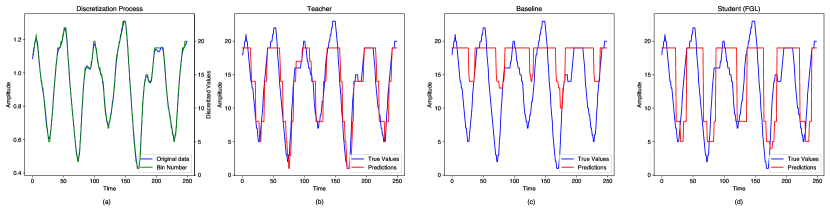
Figure 4: (a) Discretization Process of Mackey Glass. After data generation, each target value $X_{t+n}$ is assigned to a discrete value based on the number of bins and the range of data. Moreover, the number of output neurons matches the number of bins, such that each bin is treated as a separate class label. (b) Teacher model performs next-step prediction. (c) Baseline model forecasts $5$ steps into the future. (d) Student model with FGL also forecasts $5$ steps into the future. FGL allows the student model to capture neighboring spatial information of the target, leading to lower MAE loss and better learning.

Furthermore, to better suit the needs of regression, we reformulate the goals of the teacher and student models. Namely, the teacher performs next-step forecasting while the student performs long-term forecasting. This difference in forecasting horizons more concretely enforces the timescale variance between models.

As a result of this reformulation, it would be impractical to give the teacher the student data at time $x_{n}$, as the teacher associates this input with the next time step $x_{n+1}$. Rather, we give the teacher the input data previous to the student’s target,the data at $x_{n+t-1}$, such that the student and teacher models are both forecasting to the identical target value, $x_{n+t}$.

Similar to event prediction, a teacher model is first pretrained, inference is performed within the student training loop, and the loss defined by Equation (1) is computed. During testing of models we only consider the neuron with highest probability and take the corresponding MAE loss, as this is more conducive to traditional regression evaluation technique.

We test the scenario where $\alpha=0.5$ vs $\alpha=0.0$ in order to compare the effect on the student learner of only using the teacher’s uncertainty vs standard FGL. For our experiments, we utilized a one-layer recurrent-neural-network (RNN), a temperature of $T=2$, a batch size of 1, and trained the teacher model for 20 epochs while the student and baseline used 15.

5.2 Forecasting Discussion

When compared to the baseline method, FGL shows a 10% decrease in MAE loss on average across all horizons. FGL performs the strongest at longer-term horizons, while performing at par with the baseline at shorter term ones. This is likely due to the lack of information transferred from the teacher model at shorter term horizons; i.e. when the teacher is further ahead of the student, it is better able to transfer useful information due to the positional gap.

One disadvantage present in our formulation of regression forecasting is the discretization, as this process leads to a loss of precision in network prediction. To better suit traditional forecasting methodology, other uncertainity quantification methods must be used which don’t require discretization.

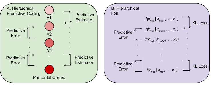
Figure 5: (A) Illustration of predictive coding in the brain. Information is received by the primary visual cortex (V1), which then propagates to different areas of the brain with more complex levels of abstraction. This propagation takes the form as a predictive estimator: higher level areas aid in prediction of lower level areas. The difference between the prediction and true output is the predictive error. Areas with lighter colors represent low-level abstractions, where darker colors represent the increasing representational demand (thoughts, movement, etc). (B) Hierarchical FGL propagates information via uncertainty, in other words, FGL substitutes the predictive estimator with the uncertainty of each layer. This uncertainty is conveyed via the KL divergence of between each layer’s probability distribution with the successive layer. The difference between each layer’s prediction and true output is the predictive error. In both models, areas lower in the hierarchy process information in a delayed manner, as they are the last to receive it. As the demand for complexity increases, so does the predictive error.

6 Future-Guided Learning And Predictive Coding

The teacher and student models can be described more acutely by Bayesian prediction. Consider a network $f(x_{t+n}|x_{t+n-1}...x_{1})$ whose goal is to predict the next step $x_{t+n}$ from the previous point $x_{t+n-1}$. The states of the network up till this point can be described by a sum of the likelihood $f(x|\theta)$ and current posterior distribution $\pi(\theta)$. In simple terms, the network makes a decision based on the gathered information up till the current point.

$${\rm teacher}=f(x_{t+n}|x_{t+n-1},x_{t+n-2}...x_{1})=\sum f(x_{t+n}|\theta)*\pi(\theta|x_{1}..x_{t+n-1})$$ (3)

$${\rm student}=f(x_{t+n}|x_{t},x_{t-1}...x_{1})=\sum f(x_{t}|\theta)*\pi(\theta|x_{1}..x_{t})$$ (4)

Consequently, the KL divergence between models then becomes:

$$D_{KL}(\rm teacher||student)=\sum f(x_{t+n}|x_{t+n-1},...x_{1})*\log(\frac{f(x_{t+n}|x_{t+n-1},...x_{1})}{f(x_{t+n}|x_{t},...x_{1})})$$ (5)

The intuition of the KL divergence arises when looking at the posterior distributions of the student and teacher. The student, when making a prediction about the future, is considerably less informed than the teacher model, which has seen an additional $n-1$ points up until its current position, and therefore has a more well-informed posterior distribution. Since the posterior directly affects a model’s probability distribution of each model, the KL divergence conveys to the student the "well-informedness" of the teacher model. As we forecast further into the future, the representational complexity of the student learner increases drastically, as it must account for more chaoticness in the data.

Using this newfound knowledge, we can extend this duality by implementing a student-teacher dynamic in between the topmost model’s current timestep $x_{n+t-1}$ and the bottom most model’s current timestep $x_{t}$. Rather than having the topmost model distill knowledge directly to the bottom most layer, we propose chaining uncertainty downwards. In other words, the model at time $x_{n+t-1}$ acts as a teacher to the model at $x_{n+t-2}$, which acts as a teacher to the model at $x_{n+t-3}$ and so on and so forth. Within the hierarchy, each model at each prediction horizon $x_{n},x_{n+1},...$ has a different timescale, and therefore, a different temporal representation.

This is strikingly similar to a potential implementation of hierarchical predictive coding in the brain. In the same vein, cortical areas which handle low-level sensory information, such as the primary visual cortex (V1), are akin to the topmost model in hierarchical FGL: $f(x_{n+t}|x_{n+t-1},...)$. Likewise, areas which handle more complex representations, such as the prefrontal cortex, are akin to the student model,$f(x_{n+t}|x_{n},...)$, as both learn abstract patterns and receive delayed temporal information. A visualization can be seen in Figure 5.

Practically speaking, viewing the teacher as a true Bayesian posterior is unrealistic, as the posterior is intractable. One solution to this dilemma is variational inference, in which a network must adjust the parameters of a surrogate distribution to approximate the posterior [19, 3]. We can more aptly view the teacher model as a well-posed surrogate distribution $T\approx q(v)$, and the student model as a prior distribution $S=p(v)$. When the teacher is able to closely model a true posterior, the loss difference between the student and teacher can provide useful information to the student model. For the teacher surrogate to closely approximate the posterior, we define a metric of difference, such as KL divergence:

$$KL(q(v),p(v|u)) =\int{q(v)\ln\frac{q(v)}{p(v|u)}dv}$$ (6)

$$=\int q(v)\ln\frac{q(v)}{p(u,v)}dv+\ln p(u)$$

the left-hand term is called the free-energy $F$ ([19]), and can be used to rewrite this variational inference procedure as:

$$\ln p(u)=-F+KL(q(v),p(v|u))$$ (7)

The term $\ln p(u)$ represents the "surprise" of the student, and is directly related to its uncertainty. Since the KL divergence is always positive, $F$ serves as a lower bound for the surprise $\ln p(u)$. Therefore, maximizing $F$ is equivalent to minimizing the prior surprise $\ln p(u)$, thereby improving the approximation of the surrogate $q(v)$. Additionally, we can characterize the transfer of information between the two models by approximating model uncertainty based on predictive errors:

$$\ln p(u)\approx\frac{1}{2}\left[-\ln\Sigma_{p}-\frac{(\Phi-v_{p})^{2}}{\Sigma_{p}}-\ln\Sigma_{u}-\frac{(u-g(\Phi))^{2}}{\Sigma_{u}}\right]$$ (8)

whose dynamics can be characterized as a system that converges onto internal representations of the input (see Appendix C).

7 Conclusion

In this paper, we introduced an unconventional way to perform time-series forecasting and event prediction by leveraging time-variance. We utilized Future-Guided Learning (FGL) to enable a future-teacher model to provide assistance to a past-student model. On biomedical signal analysis, our method results in a 50% increase in AUCROC, and on time-series forecasting, a 20% decrease in MAE loss is observed.

Despite these observed capabilities, we believe our method has many areas of improvement, especially in regards to improving efficiency and further generality across architectures. For one, training a future-model solely to assist a separate past model may be energy inefficient. It may be potentially more convenient to train a model across multiple time-horizons, wherein the shorter horizons distill information when performing inference on longer ones. Moreover, further generality may be achieved by more robust information extraction methods which are task-agnostic, such as weight comparisons.

It is important to recognize that Knowledge Distillation is only one of many ways of leveraging time variance. In time-series forecasting especially, there are many uses of information in which a future model could aid a model in the past, such as moving averages, seasonal trends, and local spatial information. For methods more in line with Knowledge Distillation, it will be valuable to consider other uncertainty quantification methods which don’t require discretization, such as Bayesian models and Monte Carlo Dropout.

Nevertheless, utilizing future-guidance in forecasting and event-prediction presents a new and unexplored paradigm in the field. Our work demonstrates the potential of this approach, and we believe it will inspire future research into more efficient, general, and adaptable methods for leveraging temporal variance to improve predictive performance.

Appendix A Additional Seizure Information

A.1 Epilepsy Background Information

Epilepsy is a neurological condition which affects millions of people worldwide. It is characterized by a rapid firing in brain activity, often leading to spasms and involuntary muscle movements. Events of epilepsy are referred to as "ictal" events, whereas pre-seizure and non-seizure periods are referred to as "preictal" and "interictal" respectively [2].

Due to the unpredictable nature of seizures, there has been a widespread effort for decades to create accurate seizure prediction mechanisms [1, 25]. However, attempts to do so have faced many challenges due to patient specificity, high noise of signals, and randomness of seizure events. To further complicate the task, there has been contradicting evidence regarding the relationship between preictal and ictal events, meaning prediction may theoretically be impossible in some cases [16].

Patients with epilepsy who are undergoing medical treatment are typically monitored via scalp EEG, in which a varying number of nodes are placed on the patients head according to the 10-20 international standard [13]. Clinicians are monitored with analyzing these signals actively, and can sound an alarm when a seizure takes place to alert medical staff. Having an accurate seizure forecasting mechanism can help alleviate this burden on hospitals, and ensure early medical intervention [16].

A.2 Seizure Data Preprocessing

Our prepossessing pipeline of EEG data is as follows. Patient data is classified into three separate categories: interictal, preictal, and ictal. With respect to preictal data, we use a seizure occurrence period of 30 minutes, and a seizure prediction horizon of 5 minutes. Data up to 5 minutes prior to seizure onset is concealed from the student, and the 30 minutes prior to this is labeled as preictal data [30]. Due to this restriction, patients whose preictal data was not long enough were omitted from the dataset.

For data processing on all classes, we perform a short-time-fourier transform (STFT) with a window size of 30 seconds. On both preictal and ictal data, we apply oversampling by taking a sliding window of STFTs. These overlapping samples exist to give the models more data on the target class, and are removed in the testing set. Our train-test-split was created by concatenating all of the interictal data, and evenly distributing them between ictal or preictal periods. The last 35% of seizures, as well as their corresponding interictal data, are used for testing. No shuffling was performed during any of these processes.

Our model of choice for both datasets was a CNN-LSTM. We used two sets of Conv3d layers, an LSTM with three hidden layers, and two linear layers.The temporal variance of LSTMs is crucial for FGL working, as without an LSTM, the network would only capture spatial data and fail to learn the temporal relation between ictal/preictal and interictal periods. All models for the remainder of the paper were trained using an NVIDIA RTX 4080 GPU.

A.3 Experimental Details and SOTA Comparison

A FGL ablation study was obtained from a full parameter sweep of alpha in increments of 0.1. From the best alpha for each patient, the sensitivity, FPR, and AUCROC are calculated over 3 trials. Temperature was set at 4, and the SGD optimizer was used with $lr=5\times 10^{-4}$ and a momentum of 0.9. Thresholds for calculating the sensitivity and FPR come from Youden’s J statistic. Best scores for each patient are bolded.

Given the non-shuffled data scheme, as well as the mix of long interictal periords between preictal ones, it is possible to infer that FGL is best utilized in a realistic online-setting, where data is being streamed. The streamlining induces further complexity to the task, as the network must not only be able to identify individual EEG signals, but correlate them with short-to-long term previously seen ones. On the other hand, the traditional approach for seizure prediction involves shuffling data and treating it as a classification problem, which fails to capture the underlying temporal nature of the data.

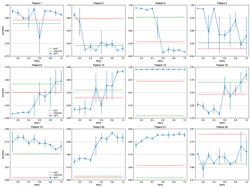
Figure 6: CHBMIT ablation study on alpha. MViT results are represented as a dashed red line, and CNNLSTM results as a dashed green line.

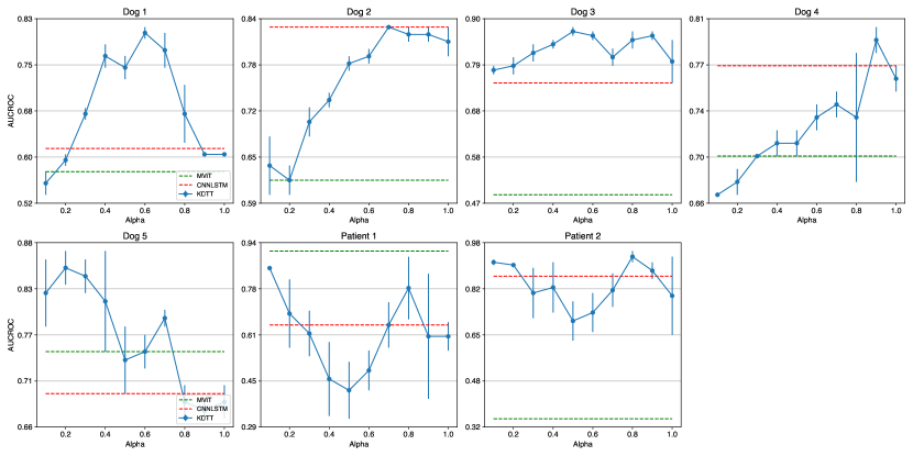
Figure 7: AES ablation study on alpha. MViT results are represented as a dashed red line, and CNNLSTM results as a dashed green line.

Table 1: CHBMIT Comparison with SOTA

MViT CNNLSTM FGL Patient FPR Sensitivity AUCROC FPR Sensitivity AUCROC FPR Sensitivity AUCROC 1 0.02_±0.02 0.82_±0.22 0.90_±0.12 0.11_±0.12 0.88_±0.10 0.92_±0.07 0.04_±0.01 0.89_±0.04 0.98_±0.01 2 0.63_±0.45 0.66_±0.47 0.15_±0.19 0.35_±0.33 0.89_±0.15 0.78_±0.17 0.10_±0.04 0.83_±0.18 0.88_±0.05 3 0.16_±0.04 0.66_±0.23 0.78_±0.15 0.42_±0.40 0.49_±0.41 0.27_±0.19 0.01_±0.01 0.90_±0.02 0.97_±0.01 5 0.61_±0.43 0.66_±0.47 0.25_±0.10 0.65_±0.46 0.67_±0.47 0.12_±0.10 0.07_±0.00 0.97_±0.01 0.96_±0.01 9 0.20_±0.16 0.41_±0.41 0.54_±0.21 0.64_±0.45 0.67_±0.47 0.42_±0.10 0.60_±0.04 0.94_±0.02 0.57_±0.18 10 0.25_±0.17 0.48_±0.13 0.53_±0.17 0.56_±0.38 0.61_±0.34 0.41_±0.13 0.26_±0.04 0.65_±0.07 0.81_±0.03 13 0.18_±0.14 0.67_±0.36 0.61_±0.32 0.11_±0.10 0.99_±0.01 0.90_±0.10 0.00_±0.00 0.99_±0.01 1.00_±0.00 18 0.30_±0.10 0.68_±0.15 0.69_±0.07 0.54_±0.28 0.64_±0.26 0.51_±0.03 0.43_±0.14 0.88_±0.06 0.69_±0.15 19 0.07_±0.05 0.47_±0.33 0.66_±0.23 0.80_±0.04 0.97_±0.01 0.50_±0.07 0.48_±0.10 0.89_±0.07 0.76_±0.03 20 0.38_±0.07 0.98_±0.03 0.67_±0.09 0.45_±0.03 0.95_±0.06 0.66_±0.07 0.13_±0.03 0.86_±0.02 0.94_±0.01 21 0.60_±0.03 1.00_±0.00 0.54_±0.03 0.49_±0.14 0.97_±0.02 0.64_±0.18 0.12_±0.02 0.73_±0.04 0.90_±0.02 23 0.62_±0.06 1.00_±0.00 0.43_±0.02 0.20_±0.27 0.92_±0.12 0.84_±0.22 0.50_±0.08 1.00_±0.00 0.67_±0.21 AVG 0.33_±0.21 0.70_±0.19 0.56_±0.20 0.44_±0.20 0.80_±0.16 0.58_±0.24 0.22_±0.01 0.87_±0.02 0.84_±0.15

Table 2: AES Comparison with SOTA

MViT CNNLSTM FGL Patient FPR Sensitivity AUCROC FPR Sensitivity AUCROC FPR Sensitivity AUCROC Dog 1 0.63_±0.06 0.93_±0.05 0.57_±0.00 0.62_±0.02 1.00_±0.00 0.61_±0.01 0.37_±0.05 0.99_±0.01 0.81_±0.01 Dog 2 0.22_±0.07 0.48_±0.04 0.62_±0.01 0.34_±0.03 0.93_±0.03 0.83_±0.00 0.40_±0.02 0.93_±0.01 0.83_±0.00 Dog 3 0.82_±0.16 0.87_±0.17 0.49_±0.02 0.35_±0.17 0.73_±0.05 0.75_±0.07 0.20_±0.08 0.71_±0.07 0.87_±0.01 Dog 4 0.36_±0.08 0.66_±0.08 0.70_±0.02 0.35_±0.05 0.83_±0.05 0.77_±0.01 0.35_±0.02 0.87_±0.02 0.79_±0.01 Dog 5 0.37_±0.04 0.93_±0.02 0.75_±0.02 0.47_±0.03 0.97_±0.01 0.70_±0.01 0.27_±0.07 0.88_±0.00 0.85_±0.02 Human 1 0.20_±0.07 0.89_±0.03 0.91_±0.04 0.51_±0.16 0.91_±0.09 0.65_±0.17 0.28_±0.01 0.96_±0.02 0.85_±0.00 Human 2 0.98_±0.00 1.00_±0.00 0.35_±0.01 0.21_±0.08 0.82_±0.10 0.86_±0.07 0.28_±0.13 0.90_±0.06 0.93_±0.02 AVG 0.51_±0.28 0.82_±0.16 0.63_±0.15 0.40_±0.12 0.88_±0.08 0.78_±0.06 0.30_±0.02 0.89_±0.01 0.85_±0.01

Appendix B Mackey Glass Results

Table 3: FGL Results on Mackey Glass

	Bins = 25			Bins = 50
Horizon	Baseline	$\alpha=0.5$	$\alpha=0.0$	Baseline	$\alpha=0.5$	$\alpha=0.0$
2	0.751±0.025	0.708±0.016	0.680±0.005	2.697±0.303	2.349±0.037	2.249±0.056
5	1.477±0.010	1.404±0.038	1.403±0.014	4.462±0.252	4.774±0.050	4.532±0.111
8	1.823±0.037	1.767±0.020	1.701±0.024	5.322±0.158	5.220±0.153	5.092±0.172
11	1.829±0.064	1.825±0.058	1.790±0.050	5.352±0.168	5.300±0.109	5.239±0.220
14	1.607±0.008	1.599±0.023	1.544±0.021	4.829±0.143	4.528±0.022	4.603±0.144
17	1.195±0.031	1.200±0.038	1,232±0.122	3.750±0.220	3.379±0.095	3.556±0.248
20	1.000±0.254	0.733±0.034	0.727±0.016	3.618±0.199	2.501±0.219	2.636±0.248
23	0.608±0.016	0.589±9.005	0.589±0.010	3.155±0.346	2.076±0.076	2.029±0.075
26	1.151±0.036	1.116±0.049	0.968±0.016	3.903±0.329	3.416±0.300	3.876±0.131
29	1.535±0.041	1.375±0.075	1.305±0.013	4.576±0.158	4.498±0.141	4.824±0.109
Avg	1.302±0.412	1.236±0.419	1.202±0.418	4.137±0.898	3.809±1.140	3.866±1.146

Appendix C FGL and Predictive Coding

Before linking FGL to predictive coding, it is valuable to review the mathematical intuition of the latter theory, which has been explored in a number of publications [19, 3]. Following these mathematical formalisms, we summarize relevant parts of these computations in this Appendix in order to link them to FGL. Namely, this can be done by defining a predictive coding network as an ensemble of units that computes the posterior probabilities of the environment $p(v|u)$, based on a (top-down) prior $p(v)$ and a (bottom-up) likelihood $p(u|v)$. Under a Gaussian assumption of these distributions, and through Bayes’ theorem, this involves computing the following:

$$p(v|u)=\frac{p(v)p(u|v)}{p(u)}=\frac{\frac{1}{\sqrt{2\pi\Sigma_{p}}}\exp{\frac{(v-v_{p})^{2}}{2\Sigma_{p}}}\frac{1}{\sqrt{2\pi\Sigma_{u}}}\exp{\frac{(u-g(v))^{2}}{2\Sigma_{u}}}}{\int p(v)p(u|v)dv}.$$ (9)

where $v$ denotes is an actual scalar value of the environment, which can be described by $v_{p}$ and $\Sigma_{p}$, respectively, the mean and variance of its Gaussian distribution. Likewise, $p(u|v)$ is the likelihood, in which the scalar $u$ is the product of an activation function $g(v)$ (for instance, the reflection of light on a surface) with a variance $\Sigma_{u}$.

The denominator is a normalization term that is computationally intractable for a biological neural network, because of the need to sample every possible permutations of $p(v)$ and $p(u|v)$. One possible simplification here is through a maximum likelihood estimation (MLE), which tries to find the value of $v$ that maximizes $p(v|u)$. We define this value as $\Phi$, whose probability $p(\Phi)$ thus replaces $p(v)$ in an MLE approach. Given that term absent from the denominator in the left-hand side of 9, we can instead focus on the numerator and write its logarithm $F$ as:

$$F=\ln\left(p(\Phi)p(u|\Phi)\right)=\ln p(\Phi)+\ln p(u|\Phi)$$ (10)

We thus get:

$$F =\ln p(\Phi)+\ln p(u|\Phi)$$ (11)

$$=\ln\left(\frac{1}{\sqrt{2\pi\Sigma_{p}}}\exp{-\frac{(\Phi-v_{p})^{2}}{2\Sigma_{p}}}\right)+\ln\left(\frac{1}{\sqrt{2\pi\Sigma_{u}}}\exp{-\frac{(u-g(\Phi))^{2}}{2\Sigma_{u}}}\right)$$

$$=\ln\left(\frac{1}{\sqrt{2\pi\Sigma_{p}}}\right)+\ln\left(\exp{-\frac{(\Phi-v_{p})^{2}}{2\Sigma_{p}}}\right)+\ln\left(\frac{1}{\sqrt{2\pi\Sigma_{u}}}\right)+\ln\left(\exp{-\frac{(u-g(\Phi))^{2}}{2\Sigma_{u}}}\right)$$

$$=\ln\left(\frac{1}{\sqrt{2\pi}}\right)-\frac{1}{2}\ln\Sigma_{p}-\frac{(\Phi-v_{p})^{2}}{2\Sigma_{p}}+\ln\left(\frac{1}{\sqrt{2\pi}}\right)-\frac{1}{2}\ln\Sigma_{u}-\frac{(u-g(\Phi))^{2}}{2\Sigma_{u}}$$

$$=\frac{1}{2}\left(-\ln\Sigma_{p}-\frac{(\Phi-v_{p})^{2}}{\Sigma_{p}}-\ln\Sigma_{u}-\frac{(u-g(\Phi))^{2}}{\Sigma_{u}}\right)+C$$

In order to obtain the maximum likelihood, we can then compute the derivative of $F$ over the surrogate value $\Phi$:

$$\frac{\delta F}{\delta\Phi} =\frac{1}{2}\left(\frac{\delta}{\delta\Phi}\left(-\frac{(u-g(\Phi))^{2}}{\Sigma_{u}}\right)+\frac{\delta}{\delta\Phi}\left(-\frac{(\Phi-v_{p})^{2}}{\Sigma_{p}}\right)+\frac{\delta}{\delta\Phi}\left(-\ln\Sigma_{u}\right)+\frac{\delta}{\delta\Phi}\left(-\ln\Sigma_{p}\right)+\frac{\delta}{\delta\Phi}C\right)$$ (12)

$$=\frac{1}{2}\left(\left(-\frac{1}{\Sigma_{u}}\frac{\delta}{\delta\Phi}(u-g(\Phi))^{2})\right)+\left(-\frac{1}{\Sigma_{p}}\frac{\delta}{\delta\Phi}(\Phi-v_{p})^{2}\right)\right)$$

Applying the power rule $(f(x)^{n})^{\prime}=nf(x)^{n-1}f^{\prime}(x)$:

$$\frac{\delta F}{\delta\Phi} =\frac{1}{2}\left(\left(-\frac{1}{\Sigma_{u}}2(u-g(\Phi))\frac{\delta}{\delta\Phi}(u-g(\Phi))\right)+\left(-\frac{1}{\Sigma_{p}}2(\Phi-v_{p})\frac{\delta}{\delta\Phi}(\Phi-v_{p})\right)\right)$$ (13)

$$=\frac{1}{2}\left(\left(-\frac{1}{\Sigma_{u}}2(u-g(\Phi))\left(\frac{\delta}{\delta\Phi}u-\frac{\delta}{\delta\Phi}g(\Phi)\right)\right)+\left(-\frac{1}{\Sigma_{p}}2(\Phi-v_{p})\left(\frac{\delta}{\delta\Phi}\Phi-\frac{\delta}{\delta\Phi}v_{p}\right)\right)\right)$$

$$=\frac{1}{2}\left(\left(-\frac{1}{\Sigma_{u}}2(u-g(\Phi))(-g^{\prime}(\Phi))\right)+\left(-\frac{1}{\Sigma_{p}}2(\Phi-v_{p})\right)\right)$$

$$=\left(\frac{1}{\Sigma_{u}}(u-g(\Phi))(g^{\prime}(\Phi))\right)+\left(-\frac{1}{\Sigma_{p}}(\Phi-v_{p})\right)$$

$$=\frac{(u-g(\Phi))}{\Sigma_{u}}g^{\prime}(\Phi)+\frac{(v_{p}-\Phi)}{\Sigma_{p}}$$

For simplification purposes, this can be rewritten with two terms:

$$\epsilon_{p} =\frac{(v_{p}-\Phi)}{\Sigma_{p}}$$ (14)

$$\epsilon_{u} =\frac{(u-g(\Phi))}{\Sigma_{u}}$$

such that the derivative becomes:

$$\frac{\delta F}{\delta\Phi}=\epsilon_{u}g^{\prime}(\Phi)+\epsilon_{p}$$ (15)

We reformulate the gradient of $F$ w.r.t $\Phi$ as a learning rule:

$$\dot{\Phi}=\epsilon_{u}g^{\prime}(\Phi)-\epsilon_{p}$$ (16)

The term $\epsilon_{p}$ is referred to as the prediction error on the causes, while $\epsilon_{u}$ is called the prediction error on the states [8]. The key conceptual difference between these two terms is that $\epsilon_{p}$ measures the difference between the inferred observation and the model’s prior expectations [19], while $\epsilon_{u}$ measures the difference between the true value and the predicted value. More simply, prediction error on the causes represents errors at higher level representations, while prediction error on the states represents raw differences between inferred and real states. $F$ is called the variational free energy, and while out of the scope of this appendix, it is intuitively linked to certain useful information theoretical metrics, namely in the form of a lower bound of the model’s surprise [8].

In predictive coding, one of the goals of a model is to maximize prediction efficiency and thus minimize both sources of prediction errors. When minimal, these give a stable point of $\epsilon_{p}$ and $\epsilon_{u}$ defined as:

$$\epsilon_{p} =\frac{\Phi-v_{p}}{\Sigma_{p}}$$ (17)

$$\Sigma_{p}\epsilon_{p} =\Phi-v_{p}$$

$$\Phi-v_{p}-\Sigma_{p}\epsilon_{p} =0$$

$$\epsilon_{u} =\frac{u-g(\Phi)}{\Sigma_{u}}$$ (18)

$$\Sigma_{u}\epsilon_{u} =u-g(\Phi)$$

$$u-g(\Phi)-\varSigma_{u}\varepsilon_{u} =0$$

And thus the dynamics of a system that seeks to minimize prediction errors to infer the most likely value of $\Phi$ in an MLE approach can be described as:

$$\dot{\varepsilon_{p}} =\Phi-v_{p}-\varSigma_{p}\varepsilon_{p}$$ (19)

$$\dot{\varepsilon_{u}} =u-g(\Phi)-\varSigma_{u}\varepsilon_{u}$$

This leads us to introduce the relationship between predictive coding and FGL. Indeed, both $\varSigma_{p}$ and $\varSigma_{u}$ parametrize the uncertainty of the model. In this MLE approach, which ideally should converge onto the most likely value of the input, any model or input-bound uncertainties are discarded. In other terms, this transforms an information-rich, distribution-based computation into a point estimate, which is incompatible with FGL, as presented here.

One alternative to the MLE approach involves the utilization of a "surrogate" distribution, through a process known as variational inference [21]. Instead of facing computationally untractable normalization terms (9) or arbitrarily complex input distributions, variational inference allows using a new distribution $q(v)$, possesses a standard form that can be succinctly described by its mean and variance.

In the context of FGL, the student and teacher networks can be more precisely defined within a Bayesian framework. Here, the teacher model is represented as a well-posed surrogate $T\approx q(v)$, and the student model is represented as a prior distribution $S=p(v)$. Thus, the following equations, which relate to a surrogate distribution $q(v)$, can be understood as using the teacher model as a surrogate representation to guide the student model.

The overall approach, in predictive coding, then changes from MLE to approximating the posterior $p(v|u)$ using $q(v)$, which requires a metric of difference, or divergence, between the two distributions. Here, we used the Kullback-Leibler divergence:

$$KL(q(v),p(v|u)) =\int{q(v)\ln\frac{q(v)}{p(v|u)}dv}$$ (20)

This KL divergence also serves to compare the probability distributions of the student and teacher models in FGL. Here, however, it is implausible for a biological network to directly measure this difference due to the same issue of computational intractability of $p(v|u)$ that led us to MLE. Indeed:

$$p(v|u)=\frac{p(u,v)}{p(u)}=\frac{p(u,v)}{\int p(v)p(u|v)dv}$$ (21)

However, expanding the KL divergence using the above equations, we see the following:

$$KL(q(v),p(v|u)) =\int{q(v)\ln\frac{q(v)}{p(v|u)}dv}$$ (22)

$$=\int{q(v)\ln\frac{q(v)p(u)}{p(u,v)}dv}$$

$$=\int{q(v)\ln\frac{q(v)}{p(u,v)}dv}+\int{q(v)\ln p(u)dv}$$

given that the surrogate $q(v)$ is a probability distribution which sums up to $1$, we get:

$$KL(q(v),p(v|u))=\int{q(v)\ln\frac{q(v)}{p(u,v)}dv}+\ln p(u)$$ (23)

We can then define a term that captures the student’s prior distribution without being computationally intractable. This term, $F$, can be defined as:

$$F =\int q(v)\ln\frac{q(v)}{p(u,v)}dv$$ (24)

$$KL(q(v),p(v|u)) =F+\ln p(u)$$

since $F$ depends on the surrogate distribution $q(v)$, the parameters which minimize the distance between the surrogate $q(v)$ and the teacher’s posterior $p(v|u)$, are identical to those which maximize $F$, which in turn negates the computation of the normalization term. By replacing in $F$, we can define the right-hand term as:

$$\ln p(u)=-F+KL(q(v),p(v|u))$$ (25)

This newly derived term, $\ln p(u)$, directly relates to the information "surprise" of the student’s estimate $p(u)$ of the actual value $v$, and thus relates directly to its uncertainty. Since KL divergence is strictly positive, $F$ acts as a lower bound of the surprise $\ln p(u)$. Consequently, maximizing $F$ is akin to minimizing surprise or uncertainty of the student $\ln p(u)$, hence improving the approximation of the surrogate $q(v)$ - that is, optimizing our student model with respect to the teacher in the context of FGL.

The introduction of surprise becomes useful below to optimize the update of uncertainty parameters in the context of a network that implements predictive computations, as we can now rewrite:

$$\ln p(u) =F+KL(q(v),p(v|u))$$ (26)

$$=\frac{1}{2}\left[-\ln\Sigma_{p}-\frac{(\Phi-v_{p})^{2}}{\Sigma_{p}}-\ln\Sigma_{u}-\frac{(u-g(\Phi))^{2}}{\Sigma_{u}}\right]+C+KL(q(v),p(v|u))$$

as the KL divergence is a strictly positive term that forms a lower bound on surprise, it can be included in the constant term $C$ for simplicity’s sake.

Starting from this definition, we can now derive $F$ to optimize $v_{p}$:

$$\frac{\delta F}{\delta v_{p}} =\frac{1}{2}\left(\frac{\delta}{\delta v_{p}}\left(-\frac{(\Phi-v_{p})^{2}}{\Sigma_{p}}\right)+\frac{\delta}{\delta v_{p}}\left(-\frac{(u-g(\Phi))^{2}}{\Sigma_{u}}\right)+\frac{\delta}{\delta v_{p}}\left(-\ln\Sigma_{u}\right)+\frac{\delta}{\delta v_{p}}\left(-\ln\Sigma_{p}\right)\right)+\frac{\delta}{\delta v_{p}}C$$ (27)

$$=\frac{1}{2}\left(\frac{\delta}{\delta v_{p}}\left(-\frac{(\Phi-v_{p})^{2}}{\Sigma_{p}}\right)\right)$$

$$=\frac{1}{2}\left(\frac{1}{-\Sigma_{p}}\frac{\delta}{\delta v_{p}}(\Phi-v_{p})^{2}\right)$$

$$=\frac{1}{-\Sigma_{p}}(\Phi-v_{p})\frac{\delta}{\delta v_{p}}(\Phi-v_{p})$$

$$=\frac{1}{-\Sigma_{p}}(\Phi-v_{p})\left(\frac{\delta}{\delta v_{p}}\Phi-\frac{\delta}{\delta v_{p}}v_{p}\right)$$

$$=\frac{\Phi-v_{p}}{\Sigma_{p}}$$

The same can be done for $\Sigma_{p}$:

$$\frac{\delta F}{\delta\Sigma_{p}} =\frac{1}{2}\left(\frac{\delta}{\delta\Sigma_{p}}\left(-\frac{(\Phi-v_{p})^{2}}{\Sigma_{p}}\right)+\frac{\delta}{\delta\Sigma_{p}}\left(-\frac{(u-g(\Phi))^{2}}{\Sigma_{u}}\right)+\frac{\delta}{\delta\Sigma_{p}}\left(-\ln\Sigma_{u}\right)+\frac{\delta}{\delta\Sigma_{p}}\left(-\ln\Sigma_{p}\right)\right)+\frac{\delta}{\delta\Sigma_{p}}C$$ (28)

$$=\frac{1}{2}\left(-\frac{\delta}{\delta\Sigma_{p}}\ln\Sigma_{p}+\left(-(\Phi-v_{p})^{2}\frac{\delta}{\delta\Sigma_{p}}\frac{1}{\Sigma_{p}}\right)\right)$$

$$=\frac{1}{2}\left(-\frac{1}{\Sigma_{p}}+\left((\Phi-v_{p})^{2}\frac{\delta\Sigma_{p}}{\Sigma_{p}^{2}}\right)\right)$$

$$=\frac{1}{2}\left((\Phi-v_{p})^{2}\frac{\delta\Sigma_{p}}{\Sigma_{p}^{2}}-\frac{1}{\Sigma_{p}}\right)$$

$$=\frac{1}{2}\left(\frac{(\Phi-v_{p})^{2}}{\Sigma_{p}^{2}}-\frac{1}{\Sigma_{p}}\right)$$

Likewise, for $\Sigma_{u}$:

$$\frac{\delta F}{\delta\Sigma_{u}} =\frac{1}{2}\left(\frac{\delta}{\delta\Sigma_{u}}\left(-\frac{(\Phi-v_{p})^{2}}{\Sigma_{p}}\right)+\frac{\delta}{\delta\Sigma_{u}}\left(-\frac{(u-g(\Phi))^{2}}{\Sigma_{u}}\right)+\frac{\delta}{\delta\Sigma_{u}}\left(-\ln\Sigma_{u}\right)+\frac{\delta}{\delta\Sigma_{u}}\left(-\ln\Sigma_{p}\right)\right)+\frac{\delta}{\delta\Sigma_{u}}C$$ (29)

$$=\frac{1}{2}\left(\frac{\delta}{\delta\Sigma_{u}}\left(-\frac{(u-g(\Phi))^{2}}{\Sigma_{u}}\right)-\frac{\delta}{\delta\Sigma_{u}}\ln\Sigma_{u}\right)$$

$$=\frac{1}{2}\left(-(u-g(\Phi))^{2}\frac{\delta}{\delta\Sigma_{u}}\frac{1}{\Sigma_{u}}-\frac{\delta}{\delta\Sigma_{u}}\ln\Sigma_{u}\right)$$

$$=\frac{1}{2}\left(-(u-g(\Phi))^{2}\frac{\delta}{\delta\Sigma_{u}}\frac{1}{\Sigma_{u}}-\frac{1}{\Sigma_{u}}\right)$$

$$=\frac{1}{2}\left(\frac{(u-g(\Phi))^{2}}{\Sigma_{u}^{2}}-\frac{1}{\Sigma_{u}}\right)$$

Yielding the learned parameters of a predictive coding network that performs equivalent computation to FGL as:

$$\frac{\delta F}{\delta v_{p}} =\frac{\Phi-v_{p}}{{\Sigma_{p}}}=\epsilon_{p}$$ (30)

$$\frac{\delta F}{\delta\Sigma_{p}} =\frac{1}{2}\left(\frac{(\Phi-v_{p})^{2}}{{\Sigma_{p}^{2}}}-\frac{1}{{\Sigma_{p}}}\right)=\frac{1}{2}\left(\epsilon_{p}^{2}-{\Sigma_{p}^{-1}}\right)$$

$$\frac{\delta F}{\delta\Sigma_{u}} =\frac{1}{2}\left(\frac{(u-g(\Phi))^{2}}{{\Sigma_{u}^{2}}}-\frac{1}{{\Sigma_{u}}}\right)=\frac{1}{2}\left(\epsilon_{u}^{2}-{\Sigma_{u}^{-1}}\right)$$

While these equations follow scalar notations, we use the same reasoning as Bogacz [3], who provides an extension to vector and matrix forms, with possible neurobiological plausible implementations.

References

- [1] Abbasi, B., Goldenholz, D.M.: Machine learning applications in epilepsy. Epilepsia 60(10), 2037–2047 (2019)
- [2] Beghi, E., Giussani, G., Nichols, E., Abd-Allah, F., Abdela, J., Abdelalim, A., Abraha, H.N., Adib, M.G., Agrawal, S., Alahdab, F., et al.: Global, regional, and national burden of epilepsy, 1990–2016: a systematic analysis for the global burden of disease study 2016. The Lancet Neurology 18(4), 357–375 (2019)
- [3] Bogacz, R.: A tutorial on the free-energy framework for modelling perception and learning. Journal of mathematical psychology 76, 198–211 (2017)
- [4] Brinkmann, B.H., Wagenaar, J., Abbot, D., Adkins, P., Bosshard, S.C., Chen, M., Tieng, Q.M., He, J., Muñoz-Almaraz, F., Botella-Rocamora, P., et al.: Crowdsourcing reproducible seizure forecasting in human and canine epilepsy. Brain 139(6), 1713–1722 (2016)
- [5] Bucila, C., Caruana, R., Niculescu-Mizil, A.: Model compression. In: Proceedings of the 12th ACM SIGKDD International Conference on Knowledge Discovery and Data Mining (KDD ’06) (2006)
- [6] Chebotar, Y., Waters, A.: Distilling knowledge from ensembles of neural networks for speech recognition. In: Interspeech. pp. 3439–3443 (2016)
- [7] Choi, K., Kersner, M., Morton, J., Chang, B.: Temporal knowledge distillation for on-device audio classification. In: ICASSP 2022-2022 IEEE International Conference on Acoustics, Speech and Signal Processing (ICASSP). pp. 486–490. IEEE (2022)
- [8] Friston, K.: A theory of cortical responses. Philosophical transactions of the Royal Society B: Biological sciences 360(1456), 815–836 (2005)
- [9] Friston, K.: Does predictive coding have a future? Nature neuroscience 21(8), 1019–1021 (2018)
- [10] Gou, J., Yu, B., Maybank, S.J., Tao, D.: Knowledge distillation: A survey. International Journal of Computer Vision 129(6), 1789–1819 (2021)
- [11] Hinton, G., Vinyals, O., Dean, J.: Distilling the knowledge in a neural network. arXiv preprint arXiv:1503.02531 (2015)
- [12] Huang, M., You, Y., Chen, Z., Qian, Y., Yu, K.: Knowledge distillation for sequence model. In: Interspeech. pp. 3703–3707 (2018)
- [13] Jasper, H.H.: Ten-twenty electrode system of the international federation. Electroencephalogr Clin Neurophysiol 10, 371–375 (1958)
- [14] Kaggle: Upenn and mayo clinic’s seizure detection challenge. https://www.kaggle.com/c/seizure-detection (2014)
- [15] Keller, G.B., Mrsic-Flogel, T.D.: Predictive processing: a canonical cortical computation. Neuron 100(2), 424–435 (2018)
- [16] Kuhlmann, L., Lehnertz, K., Richardson, M.P., Schelter, B., Zaveri, H.P.: Seizure prediction—ready for a new era. Nature Reviews Neurology 14(10), 618–630 (2018)
- [17] Liang, C., Zuo, S., Zhang, Q., He, P., Chen, W., Zhao, T.: Less is more: Task-aware layer-wise distillation for language model compression. In: International Conference on Machine Learning. pp. 20852–20867. PMLR (2023)
- [18] Lotter, W., Kreiman, G., Cox, D.: Deep predictive coding networks for video prediction and unsupervised learning. arXiv preprint arXiv:1605.08104 (2016)
- [19] Millidge, B., Seth, A., Buckley, C.L.: Predictive coding: a theoretical and experimental review. arXiv preprint arXiv:2107.12979 (2021)
- [20] Millidge, B., Tschantz, A., Buckley, C.L.: Predictive coding approximates backprop along arbitrary computation graphs. Neural Computation 34(6), 1329–1368 (2022)
- [21] Murphy, K.P.: Machine learning: a probabilistic perspective. MIT press (2012)
- [22] Oord, A.v.d., Li, Y., Vinyals, O.: Representation learning with contrastive predictive coding. arXiv preprint arXiv:1807.03748 (2018)
- [23] Rao, R.P., Ballard, D.H.: Predictive coding in the visual cortex: a functional interpretation of some extra-classical receptive-field effects. Nature neuroscience 2(1), 79–87 (1999)
- [24] Shoeb, A.H., Guttag, J.V.: Application of machine learning to epileptic seizure detection. In: Proceedings of the 27th international conference on machine learning (ICML-10). pp. 975–982 (2010)
- [25] Siddiqui, M.K., Morales-Menendez, R., Huang, X., Hussain, N.: A review of epileptic seizure detection using machine learning classifiers. Brain informatics 7(1), 5 (2020)
- [26] Spratling, M.W.: Predictive coding as a model of response properties in cortical area v1. Journal of neuroscience 30(9), 3531–3543 (2010)
- [27] Spratling, M.W.: A hierarchical predictive coding model of object recognition in natural images. Cognitive computation 9(2), 151–167 (2017)
- [28] Tran, V., Wang, Y., Zhang, Z., Hoai, M.: Knowledge distillation for human action anticipation. In: 2021 IEEE International Conference on Image Processing (ICIP). pp. 2518–2522. IEEE (2021)
- [29] Truong, N.D., Kuhlmann, L., Bonyadi, M.R., Yang, J., Faulks, A., Kavehei, O.: Supervised learning in automatic channel selection for epileptic seizure detection. Expert Systems with Applications 86, 199–207 (2017)
- [30] Truong, N.D., Nguyen, A.D., Kuhlmann, L., Bonyadi, M.R., Yang, J., Ippolito, S., Kavehei, O.: Convolutional neural networks for seizure prediction using intracranial and scalp electroencephalogram. Neural Networks 105, 104–111 (2018)
- [31] Tscshantz, A., Millidge, B., Seth, A.K., Buckley, C.L.: Hybrid predictive coding: Inferring, fast and slow. PLoS Computational Biology 19(8), e1011280 (2023)
- [32] Von Helmholtz, H.: Handbuch der physiologischen Optik, vol. 9. Voss (1867)
- [33] Xu, X., Li, M., Tao, C., Shen, T., Cheng, R., Li, J., Xu, C., Tao, D., Zhou, T.: A survey on knowledge distillation of large language models. arXiv preprint arXiv:2402.13116 (2024)
- [34] Yang, Y., Truong, N.D., Eshraghian, J.K., Nikpour, A., Kavehei, O.: Weak self-supervised learning for seizure forecasting: a feasibility study. Royal Society Open Science 9(8), 220374 (2022)
- [35] Zhang, Y., Liu, L., Liu, L.: Cuing without sharing: A federated cued speech recognition framework via mutual knowledge distillation. In: Proceedings of the 31st ACM International Conference on Multimedia. pp. 8781–8789 (2023)