CosFairNet:A Parameter-Space based Approach for Bias Free Learning

Abstract

Deep neural networks trained on biased data often inadvertently learn unintended inference rules, particularly when labels are strongly correlated with biased features. Existing bias mitigation methods typically involve either a) predefining bias types and enforcing them as prior knowledge or b) reweighting training samples to emphasize bias-conflicting samples over bias-aligned samples. However, both strategies address bias indirectly in the feature or sample space, with no control over learned weights, making it difficult to control the bias propagation across different layers. Based on this observation, we introduce a novel approach to address bias directly in the model’s parameter space, preventing its propagation across layers. Our method involves training two models: a bias model for biased features and a debias model for unbiased details, guided by the bias model. We enforce dissimilarity in the debias model’s later layers and similarity in its initial layers with the bias model, ensuring it learns unbiased low-level features without adopting biased high-level abstractions. By incorporating this explicit constraint during training, our approach shows enhanced classification accuracy and debiasing effectiveness across various synthetic and real-world datasets of different sizes. Moreover, the proposed method demonstrates robustness across different bias types and percentages of biased samples in the training data. The code is available at: https://visdomlab.github.io/CosFairNet/

1 Introduction

In recent times, there has been a growing concern about the latent possibilities of growing bias and fairness issues within artificial intelligence (AI), deep learning frameworks and models. Bias can infiltrate AI frameworks during various stages, starting from data acquisition, extending to model creation and algorithm development, and even up to the deployment stage [Torralba and Efros(2011)]. The increasing use of deep learning models in various sensitive and high-impact applications makes it extremely crucial to identify and mitigate bias at all potential stages to ensure the development of fair and trustworthy AI workflows [Mehrabi et al.(2021)Mehrabi, Morstatter, Saxena, Lerman, and Galstyan].

Deep learning models tend to learn easy-to-learn features and attributes much faster than hard-to-learn features such as actual shapes and high-level abstraction of an object [Nam et al.(2020)Nam, Cha, Ahn, Lee, and Shin, Geirhos et al.(2018)Geirhos, Rubisch, Michaelis, Bethge, Wichmann, and Brendel]. For instance, while training a cow classifier, the model may fail to classify the cow if it is placed on the surface of a lake or on a beach. This happens because the model has a contextual bias, and to make a confident prediction, the correct context, typically a green grassland, is required. The absence of a non-correlating background or context results in incorrect prediction. The deep networks are prone to noise memorization faster and quicker than their intended purpose [Arpit et al.(2017)Arpit, Jastrzkebski, Ballas, Krueger, Bengio, Kanwal, Maharaj, Fischer, Courville, Bengio, et al.]. The models often suppress shapes and learn color [Dosovitskiy et al.(2014)Dosovitskiy, Springenberg, Riedmiller, and Brox], texture [Geirhos et al.(2018)Geirhos, Rubisch, Michaelis, Bethge, Wichmann, and Brendel] and attribute bias [Hooker et al.(2020)Hooker, Moorosi, Clark, Bengio, and Denton]. Henceforth, the model is dependent on bias and so performs better on in-bias or bias-aligned samples and fails to perform as soon as there is a bias shift or as the non-correlated data samples are encountered. A classic example of this is a cow in a green pasture and a camel in a desert. If the backgrounds of these images are exchanged, the model’s performance drops drastically [Beery et al.(2018)Beery, Van Horn, and Perona]. These unintended bias leads the trained model to make erroneous inferences by relying on shortcuts.

Figure 1: Gradient activation map of biased and debiased models in lower and higher layers for the BFFHQ dataset. (a) and (b) illustrate gender predictions of the biased and debiased models at the initial layer. It is evident that the debiased model closely corresponds to the biased model. In contrast, (c) and (d) show no correspondence as the learned weights differ at the higher layer. (Best view in color).

Current methods for bias removal use various approaches. A substantial body of research relies on explicit bias annotations [Kim et al.(2019)Kim, Kim, Kim, Kim, and Kim, Li and Vasconcelos(2019), Sagawa et al.(2019)Sagawa, Koh, Hashimoto, and Liang, Teney et al.(2020)Teney, Abbasnejad, and van den Hengel, Krueger et al.(2021)Krueger, Caballero, Jacobsen, Zhang, Binas, Zhang, Le Priol, and Courville, Bai et al.(2021)Bai, Sun, Hong, Zhou, Ye, Ye, Chan, and Li]. However, this reliance on explicit annotations can be costly and time-consuming, necessitating a thorough understanding of the potential spurious correlations between bias attributes and target labels. Another significant area of study in bias mitigation centres on algorithms that utilize reweighting techniques [Lee et al.(2021)Lee, Kim, Lee, Lee, and Choo, Nam et al.(2020)Nam, Cha, Ahn, Lee, and Shin]. These algorithms assign higher weights to the bias-conflicting samples than the bias-aligned samples during the training phase. A notable approach, among reweighting techniques, involves training two models: (a) a bias model that learns the dataset’s bias and (b) a debias model that leverages the learning of the bias model to identify bias-aligned samples and weigh them down during training phase so that a spurious correlation between bias attributes and the target label is not formed. Subsequently, in the continuation to the reweighting, several studies propose improvement by modifying the model architecture  [Lee et al.(2022)Lee, Park, Kim, Lee, Choi, and Choo, Kim et al.(2022)Kim, Hwang, Ahn, Park, and Kwak].

Although the proposed methods demonstrate their effectiveness in specific applications, they encounter some major challenges. While one type of method suffers the challenge of expressing and quantifying biases precisely for the model to handle them explicitly, another type based on sampling or re-weighting is prone to assigning disproportionately high weights to noisy or outlier samples, especially when they constitute a minority in the dataset. Furthermore, when down-weighting bias-aligned samples, these techniques also discard valuable debias features alongside the bias features, which could benefit the learning process. Moreover, relying solely on the existing re-weighting technique may introduce new spurious correlations between bias and target labels when multiple biases exist.

In this study, we address some of the existing challenges by introducing a novel method that mitigates bias in the model’s parameter space. It is observed that the learned parameters of a biased model and a debiased model at initial layers are similar, while the parameters in the final stage layers differ. To illustrate this observation, we generate the gradient activation maps [Selvaraju et al.(2017)Selvaraju, Cogswell, Das, Vedantam, Parikh, and Batra] for predictions from biased and debiased models at both initial and later layers. In Fig. 1, (a) and (b) demonstrate that both models at the initial layer utilize common features for gender prediction. In contrast, in (c) and (d), the parameters of the biased model in the later stage utilize the mouth region, while the debiased model employs other features for gender identification. Our method builds on the insights that low-level features of biased samples are not detrimental to learning, but it is the unintended correlation between biased features and target labels that poses the problem. Thus, instead of discarding low-level features of bias-aligned samples by simply down-weighting them, we propose to harness them by enforcing a (dis)similarity constraint in the parameter space of the debias and bias model. Specifically, we enforce similarity constraints on the initial layers of these models while introducing an orthogonality constraint on the final layers. The purpose of these constraints is twofold: first, to ensure the preservation of low-level features from all input samples, including bias-aligned ones, while simultaneously preventing the formation of unintended correlations with the target label. The orthogonality constraint, applied at the final layer, compels the debias model to focus on learning the signal rather than the bias. By applying this constraint in the parameter space, our method also prevents the propagation of biases through subsequent layers. Our main technical contributions are:

• We introduce a novel approach to mitigate bias by model parameter realignment, along with a unique architecture design to prevent the acquisition and propagation of bias during model training.

• We demonstrate the utility of bias-aligned samples and propose to leverage them in the model training through a simple yet effective constraint within the model’s parameter space. Further, by applying an orthogonality constraint to the later-stage layers, we direct the debias model to acquire distinct learning compared to the bias model, thus preventing spurious correlations between bias attributes and target labels.

• The proposed method demonstrates superior performance when compared to both types of approaches: those relying on bias labels and those solely based on sample re-weighting schemes across two real-world datasets and two well-controlled synthetic datasets.

2 Related Work

This section classifies prior research in the field of debiasing techniques, with a specific emphasis on reducing bias. Debiasing efforts can be categorised into two primary groups: debiasing through the utilisation of prior knowledge and debiasing approaches based on reweighting. These categories include a range of methods, each with its own distinct methodology and consequences, which are evaluated and compared to our approach.

Debiasing using prior knowledge A variety of works focus on mitigating bias through prior knowledge of bias types in datasets, utilizing bias annotations and distinct prediction heads for different biases [Wang et al.(2019)Wang, He, Lipton, and Xing, Tartaglione et al.(2021)Tartaglione, Barbano, and Grangetto, Bahng et al.(2020)Bahng, Chun, Yun, Choo, and Oh, Kim et al.(2022)Kim, Hwang, Ahn, Park, and Kwak, Sagawa et al.(2019)Sagawa, Koh, Hashimoto, and Liang, Teney et al.(2020)Teney, Abbasnejad, and van den Hengel, Krueger et al.(2021)Krueger, Caballero, Jacobsen, Zhang, Binas, Zhang, Le Priol, and Courville, K Kurmi et al.(2022)K Kurmi, Sharma, Sharma, and Namboodiri, Bai et al.(2021)Bai, Sun, Hong, Zhou, Ye, Ye, Chan, and Li, Li et al.(2023)Li, Evtimov, Gordo, Hazirbas, Hassner, Ferrer, Xu, and Ibrahim]. Some methods, like those proposed by Wang et al [Wang et al.(2019)Wang, He, Lipton, and Xing] and End et al [Tartaglione et al.(2021)Tartaglione, Barbano, and Grangetto], employ predefined representations of bias or orthogonal gradients to debias data, though these can be complex and cost-intensive to apply in real-world settings.

Debiasing using sample reweighting Reweighting-based debiasing methods involve sample weighting, label usage, or model architectures to counter biases [Kim et al.(2019)Kim, Kim, Kim, Kim, and Kim, Li and Vasconcelos(2019), Nam et al.(2020)Nam, Cha, Ahn, Lee, and Shin, Lee et al.(2021)Lee, Kim, Lee, Lee, and Choo, Vandenhirtz et al.(2023)Vandenhirtz, Manduchi, Marcinkevičs, and Vogt, Qraitem et al.(2023)Qraitem, Saenko, and Plummer, Lee et al.(2022)Lee, Park, Kim, Lee, Choi, and Choo, Kim et al.(2022)Kim, Hwang, Ahn, Park, and Kwak, Jeon et al.(2022)Jeon, Kim, Lee, Kang, and Lee]. Techniques range from dual model architectures to ensemble methods and feature-level swapping. However, methods like Bias Swap [Kim et al.(2021)Kim, Lee, and Choo] or those by Wu et al [Wu et al.(2023)Wu, Yuksekgonul, Zhang, and Zou], which rely on image translation, are limited by their complexity. Other approaches, such as those using adversarial learning or alternative loss functions [Bahng et al.(2020)Bahng, Chun, Yun, Choo, and Oh, Wang et al.(2019)Wang, He, Lipton, and Xing, Ko et al.(2023)Ko, Lee, Park, Noh, Park, and Kim], show promise but often perform similarly to conventional models.

In summary, existing debiasing techniques vary widely, from employing prior knowledge to reweighting samples and using complex model architectures. Despite their innovative approaches, these methods often face challenges related to implementation complexity, costs, and the handling of hyperparameters. Our novel approach aims to synthesise the strengths of these methodologies while overcoming their limitations to improve debiasing effectiveness.

3 Problem Formulation

We address this as a $\mathcal{N}$-class classification problem where a dataset $\mathcal{D}$ contains inputs $x$ with attributes $\{a_{1},\ldots,a_{k}\}$, each attribute $a_{i}$ taking values from a predefined set $A_{i}$. The main objective is to construct a predictive function $f$ that operates under a specific set of decision rules $\mathcal{F}_{t}$. This function $f$ aims to accurately predict the target attribute $y$, where $y=a_{t}$ and $a_{t}$ is an element of the set $A_{t}$. For the purpose of determining whether or not there is bias within the dataset $\mathcal{D}$, the following conditions are crucial:

1. Correlation Condition: There exists a non-target attribute $a_{b}$, different from $y$, that correlates significantly with $y$. This is quantitatively assessed using the conditional entropy $H(y|a_{b})$, which approaches zero, indicating that $a_{b}$ nearly determines $y$.

2. Decision Rule Condition: There is an effective alternative decision rule $s_{b}$, not included in $\mathcal{F}_{t}$, capable of classifying based on $a_{b}$. This suggests that $a_{b}$ could independently serve as a strong predictor for $y$.

When these conditions are met, $a_{b}$ is recognised as a bias attribute in $\mathcal{D}$. Furthermore, instances in $\mathcal{D}$ are classified according to their alignment with the bias attribute $a_{b}$. Bias-Aligned: An instance is considered bias-aligned if it conforms to the alternative decision rule $s_{b}$, which align with the bias observed in $a_{b}$. Bias-Conflicting: Bias-conflicting instances are those that do not conform to $s_{b}$, indicating non-typical behaviour despite a correlation between $a_{b}$ and $y$. The development of $f$ and $\mathcal{F}_{t}$ must not only achieve high prediction accuracy for $y$ but also address and mitigate the biases associated with $a_{b}$ to ensure fairness and equity in the predictive outcomes across all classes in $\mathcal{D}$.

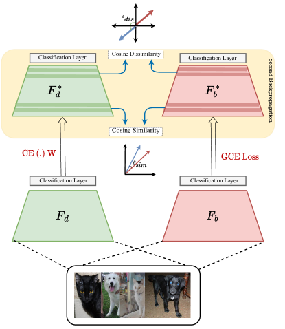
Figure 2: The architecture of CosFairNet depicts the debiasing mechanism where $F_{d}$ and $F_{b}$ are the debias and bias models, respectively. W represents the weighting of samples. Cosine similarity is employed to align (initial layers) or de-align (later layers) $F_{d}$ and $F_{b}$ model layers to ensure differentiated learning of biased and unbiased representations. In figure, $CE(.)$ stands for cross-entropy loss, $GCE(.)$ for generalized cross-entropy loss and $W$ for relative difficulty score.

4 Proposed Method

We propose a novel framework CosFairNet, that addresses the problem of bias through a principled realignment of model weights. Our approach is predicated on the use of cosine (dis)similarity measures to modulate the influence of bias, which manifests at varying magnitudes across different network layers. Specifically, we apply cosine similarity to synchronize the lower layers of the bias model $F_{b}$ with the corresponding layers of the debias model $F_{d}$, thus aligning their basic low-level feature learning. This step ensures that both models extract similar foundational details from the data. In contrast, we employ cosine dissimilarity at the last stage layers to encourage $F_{d}$ to diverge from $F_{b}$ in its high-level feature representations. During training, $F_{b}$ excels in identifying bias-aligned samples. Leveraging this, we make the initial layers of $F_{b}$ akin to those of $F_{d}$; at the same time $F_{b}$ seeks to capture biases, and $F_{d}$ aims to learn genuine features. This adversarial arrangement prompts realignment of weights that enhances the performance of both models by prioritizing features that improve $F_{d}$’s debiasing capability. Furthermore, by ensuring the model layers are constrained to the unit hyper-sphere, we measure similarity and dissimilarity using angular distance, defined as follows:

$$\textit{S}=\mathcal{L}_{cosSim}(F_{b},F_{d})=\frac{\mathcal{L}_{F_{b}}\cdot\mathcal{L}_{F_{d}}}{\|\mathcal{L}_{F_{b}}\|\cdot\|\mathcal{L}_{F_{d}}\|},$$ (1)

where $\mathcal{L}_{F_{b}}$ and $\mathcal{L}_{F_{d}}$ are the layer parameters. Given the unit norm constraint, the dot product similarity yields the cosine of the angular separation between the two parameter vectors, with $S$ ranging from 1 to -1, indicating 0-degree (aligned) to 180-degree (opposed) separations, respectively.

4.1 Model Architecture

The model architecture, as depicted in Fig. 2, is a dual model framework inspired by the two-model setup from [Nam et al.(2020)Nam, Cha, Ahn, Lee, and Shin]. The architecture consists of two parallel networks: the debiasing model $F_{d}$ and the biased model $F_{b}$, both featuring the same structural design. The training process is bifurcated into two distinct yet interconnected phases. Initially, $F_{b}$ is trained using a generalized cross entropy (GCE) loss to effectively capture bias-aligned samples. Concurrently, $F_{d}$ is trained with a weighted cross entropy (CE) loss, wherein the weights $\mathcal{W}$ are adjusted to give precedence to bias-conflicting samples. A pivotal characteristic of this architecture is the synergistic interaction between the corresponding layers of $F_{d}$ and $F_{b}$. During the second phase of training, the layers “$k$” of both models undergo a process of alignment or dealignment, contingent upon their position within the model’s layer position.

Training a biased Model Our approach to training a biased model involves employing the generalized cross entropy (GCE) loss function [Zhang and Sabuncu(2018)] to amplify the model’s unintentional decision rule. The GCE loss, defined as $GCE(p(x;\theta_{b}),y)=\frac{1-p_{y}(x;\theta_{b})^{q}}{q}$, uses $p(x;\theta_{b})$ to represent the softmax output, and $p_{y}(x;\theta_{b})$ as the probability of the target attribute $y$. The hyperparameter $q$, in the range $(0,1]$, modulates bias amplification, with $\text{lim}_{q\rightarrow 0}\frac{1-p_{y}^{q}}{q}$ mirroring standard cross entropy (CE) loss. Unlike CE loss, GCE loss’s gradient, $\frac{\partial GCE(p,y)}{\partial\theta_{b}}=p^{q}_{y}\frac{\partial CE(p,y)}{\partial\theta_{b}}$, disproportionately weighs samples where the model’s prediction strongly aligns with the target. This emphasis on “easier” samples leads to an augmented bias in the model’s learning process compared to CE-trained networks, hence giving us a strong biased model.

Training a debiased model While concurrently training a biased model as previously described, we also train a debiased model. This involves employing the CE loss with re-weighting based on a relative difficulty score $\mathcal{W}(x)$. The score is formulated as follows: $\mathcal{W}(x)=\frac{\text{CE}(F_{b}(x),y)}{\text{CE}(F_{b}(x),y)+\text{CE}(F_{d}(x),y)}$. Here, $F_{b}(x)$ and $F_{d}(x)$ represent the softmax outputs of the biased and debiased models, respectively. This score quantifies the degree to which each sample may introduce bias that conflicts or aligns with our observations. Specifically, for bias-aligned samples, where the biased model $F_{b}$ incurs a smaller loss as compared to the debiased model $F_{d}$ during early training stages, the difficulty score is low, resulting in a smaller weight for training the debiased model. Conversely, for bias-conflicting samples, where the biased model $F_{b}$ experiences a larger loss compared to the debiased model $F_{d}$, the difficulty score is high (close to 1), leading to a higher weight for training the debias model.

4.2 Realignment of Debias-Model’s Parameters

In the consequent training phase, the $F_{b}$ and $F_{d}$ models are updated with $\operatorname{GCE}(p(x;\theta_{b});y_{i})$ and $\mathcal{W}\cdot\operatorname{CE}(p(x;\theta_{d});y_{i})$ respectively. Realignment of $F_{d}$ parameters with $F_{b}$ occurs within the same batch and step, using cosine similarity as a loss function (see Eq. 1). This similarity measure ranges from $-1$ to $1$, indicating how vectors are oriented in the multidimensional space. During the second back-propagation, cosine similarity and dissimilarity are applied between the models’ layers—initial layers use similarity, while later layers use dissimilarity.

Given $F_{b}$’s ability in correctly classifying bias-aligned samples, the second updates focus solely on $F_{d}$’s layers, leaving $F_{b}$ layers unchanged. It’s worth noting that gradients flow from higher to lower layers during backpropagation. As a result, while updating the later layer of the $F_{d}$ model, the optimisers may also change the layers before the given layer due to their momentum. To correctly update the $F_{d}$ model, all layers must be frozen during the second update except the layer to be updated or their learning rate turned to zero. After the second update of $F_{d}$, the training step concludes, enhancing debiasing accuracy. The specifics of this training method are described in the algorithm and can be found in the Supplementary Material.

5 Experiments and Results

We conduct comprehensive experiments to evaluate our method across multiple datasets, including two synthetic datasets: Colored MNIST [Nam et al.(2020)Nam, Cha, Ahn, Lee, and Shin] and Corrupted CIFAR-$10^{1}$ [Nam et al.(2020)Nam, Cha, Ahn, Lee, and Shin] and two real-world datasets: BFFHQ [Kim et al.(2021)Kim, Lee, and Choo] and Dogs & Cats [Lee et al.(2022)Lee, Park, Kim, Lee, Choi, and Choo]. We first evaluate the effectiveness of our model for the classification task under different percentages of biased samples within the datasets. Subsequently, we perform additional experiments to address the following research questions:

1. How does the performance of our method change with an increasing ratio of biased samples in the training data, compared to state-of-the-art baselines?

2. What is the impact of each constraint, including similarity and dissimilarity, applied to the model’s weights on the overall performance?

3. How effective are the learned embedded features in separating target classes and distinguishing between bias and debias samples?

Datasets We evaluate our debiasing approach using four datasets. The Colored MNIST dataset, a modified version of MNIST with colored digits to induce spurious correlations, ensures consistency in dataset comparisons. The Corrupted CIFAR-$10^{1}$ dataset introduces bias through environmental distortions like fog and brightness changes. The BFFHQ dataset, derived from Flickr-Faces-HQ, uses gender as a bias to analyze age, while the Dogs & Cats dataset associates animal species with color. Further information regarding the datasets can be found in the supplementary material. Additionally, details and results on the BAR dataset [Nam et al.(2020)Nam, Cha, Ahn, Lee, and Shin] can also be found in the supplementary material.

Implementation details: We use a multi-layer perceptron (MLP) with three hidden layers for Colored MNIST, as suggested by [Nam et al.(2020)Nam, Cha, Ahn, Lee, and Shin] and [Lee et al.(2022)Lee, Park, Kim, Lee, Choi, and Choo]. For Corrupted CIFAR-$10^{1}$, we use ResNet20 and train it from scratch with random initialization. For all other datasets, we use pre-trained ResNet18 [He et al.(2016)He, Zhang, Ren, and Sun] topped with 3 MLP layers with 0.5 dropout between the layers. The Adam optimizer is used for all datasets, with a learning rate of 0.001 for all the datasets. Additionally, we keep the batch size of 256 for Colored MNIST and Corrupted CIFAR-$10^{1}$, while 64 for the BFFHQ [Kim et al.(2021)Kim, Lee, and Choo] and Dogs & Cats [Lee et al.(2022)Lee, Park, Kim, Lee, Choi, and Choo] dataset.

5.1 Q1 - Comparative performance analysis with state-of-the-art under varying bias ratios

Firstly, we analyze the effectiveness of our model on the well-controlled datasets - Colored MNIST adapted from [Nam et al.(2020)Nam, Cha, Ahn, Lee, and Shin] and Corrupted CIFAR-$10^{1}$ from [Hendrycks and Dietterich(2019)], where the bias takes the form of color and corruption, respectively. Table 2 shows the results on Colored MNIST with different bias-conflicting ratio datasets. Due to the diverse construction of the synthetic Colored MNIST dataset, we limited our analysis to methods that utilised the same dataset as ours. As stated by [Flachot and Gegenfurtner(2018)], the color and small-level features are learned in the early layers, and the information is passed on to the later layers (classification layers) of the model. Therefore, the outcome is expected to be biased in the presence of easy-to-learn bias features, such as color, while intrinsic features like the shape of the digits are suppressed.

We compare the performance of the proposed model with state-of-the-art methods. Our model consistently outperforms all the methods across all variations of bias ratios. We also benchmarked our model against the recent work AmpliBias [Ko et al.(2023)Ko, Lee, Park, Noh, Park, and Kim]. As shown in Table 2, the proposed model consistently outperforms AmpliBias across all bias ratios by varying margins. Notably, our method demonstrates robust performance, with an average improvement of $3\%$ over LFF and DisEnt, and over $9\%$ compared to AmpliBias at 95% bias ratio. Similarly, for 99.5% bias ratio, the proposed model’s improvement is 3% over LFF and DisEnt, and over $1\%$ compared to AmpliBias. We suspect that these methods struggle with ineffective sample-reweighting when minority instances are rare, as also stated in [Wu et al.(2023)Wu, Yuksekgonul, Zhang, and Zou]. However, we achieve a more balanced performance not only when trained with a very low bias-conflicting ratio but also when the bias-conflicting ratio is significantly high, a scenario often encountered in real-world applications.

	Colored MNIST [Nam et al.(2020)Nam, Cha, Ahn, Lee, and Shin]
Bias Ratio(%)	99.50	99.00	98.00	95.00
Vanilla	34.75	49.87	65.72	81.72
HEX [Wang et al.(2019)Wang, He, Lipton, and Xing]	42.25	47.02	72.82	85.50
LNL [Kim et al.(2019)Kim, Kim, Kim, Kim, and Kim]	36.29	49.48	63.30	81.30
EnD [Tartaglione et al.(2021)Tartaglione, Barbano, and Grangetto]	35.33	48.97	67.01	82.09
LFF [Nam et al.(2020)Nam, Cha, Ahn, Lee, and Shin]	63.49	72.94	80.67	85.81
DisEnt [Vandenhirtz et al.(2023)Vandenhirtz, Manduchi, Marcinkevičs, and Vogt]	63.98	76.33	82.38	85.54
AmpliBias [Ko et al.(2023)Ko, Lee, Park, Noh, Park, and Kim]	66.01	67.79	71.32	78.88
BiasEnsemble [Lee et al.(2022)Lee, Park, Kim, Lee, Choi, and Choo]	66.71	75.80	82.98	86.51
A2 [An et al.(2022)An, Kim, Ko, Lee, and Woo]	67.47	70.68	76.93	86.09
Ours	67.25	78.03	84.22	88.64

Table 1: Comparative accuracy performance (in %) on bias conflicting samples of various debiasing algorithms on the Colored MNIST dataset, with respect to different bias ratios.

	Corrupted CIFAR-$10^{1}$
Bias Ratio(%)	99.50	99.00	98.00	95.00
Vanilla	17.93	22.72	30.21	45.24
HEX [Wang et al.(2019)Wang, He, Lipton, and Xing]	15.39	16.62	17.81	21.74
ReBias [Bahng et al.(2020)Bahng, Chun, Yun, Choo, and Oh]	22.68	27.92	32.09	43.74
EnD [Tartaglione et al.(2021)Tartaglione, Barbano, and Grangetto]	20.74	24.19	38.88	40.54
A2 [An et al.(2022)An, Kim, Ko, Lee, and Woo]	23.37	27.54	30.60	37.60
DisEnt [Lee et al.(2021)Lee, Kim, Lee, Lee, and Choo]	31.97	31.22	36.98	46.40
LFF [Nam et al.(2020)Nam, Cha, Ahn, Lee, and Shin]	29.87	33.84	40.21	51.83
$\epsilon$-SupInfoNCE [Barbano et al.(2023)Barbano, Dufumier, Tartaglione, Grangetto, and Gori]	33.71	38.28	41.87	51.62
LogitCorrection [Liu et al.(2023)Liu, Zhang, Sekhar, Wu, Singhal, and Fernandez-Granda]	34.56	37.34	47.81	54.55
AmpliBias [Ko et al.(2023)Ko, Lee, Park, Noh, Park, and Kim]	34.63	45.95	48.74	52.22
Ours	36.34	43.94	50.83	60.06

Table 2: Comparative accuracy performance ( in %) on bias conflicting samples of various debiasing algorithms on the Corrupted CIFAR-$10^{1}$ dataset.

We tested our method on the CIFAR-10 dataset, which is more complex than the Colored MNIST dataset. As with CMNIST, on the Corrupted CIFAR dataset, the model tends to learn simpler features like textures [Geirhos et al.(2018)Geirhos, Rubisch, Michaelis, Bethge, Wichmann, and Brendel, Arpit et al.(2017)Arpit, Jastrzkebski, Ballas, Krueger, Bengio, Kanwal, Maharaj, Fischer, Courville, Bengio, et al.] over intrinsic features. Table 2 shows our results on the Corrupted CIFAR-$10^{1}$ dataset. Despite the dataset’s difficulty, our method outperforms most current models, including recent advancements that focus on bias mitigation through logit correction loss minimization [Liu et al.(2023)Liu, Zhang, Sekhar, Wu, Singhal, and Fernandez-Granda]. Introducing orthogonality constraints in the parameter space significantly enhances performance, even when biases such as low-level texture features are present. This improvement may stem from biases in the initial layers not transferring to the final layers, as the debiased model $F_{d}$ starts similar to $F_{b}$ but becomes significantly different, leading to an unbiased model.

Our model excels across various bias-conflicting ratios, surpassing most other models [Liu et al.(2023)Liu, Zhang, Sekhar, Wu, Singhal, and Fernandez-Granda, Park et al.(2023)Park, Lee, and Ye, Barbano et al.(2023)Barbano, Dufumier, Tartaglione, Grangetto, and Gori], except at a $99\%$ bias ratio, where Amplibias has a slight $2.01\%$ lead. We believe our model’s success is due to its ability to utilize low-level features effectively while preventing false correlations between targets and biases by implementing orthogonality constraints.

In Table  4 and Table  4, we present an evaluation of our proposed method against state-of-the-art algorithms on two distinct real-world datasets BFFHQ and Cats $\&$ Dogs respectively. BFFHQ exhibits facial attributes as bias, while Cats $\&$ Dogs involve image bias (color in the image). Similar to synthetic datasets, our method consistently outperforms all baselines, including recent ones, by a significant margin. As presented in Table 4, our model achieves a notable improvement in accuracy, gaining $12.58\%$ at the $99.00\%$ bias ratio and $7.9\%$ improvement at the $95.00\%$ bias ratio. Moreover, the improvement is substantial (around $35\%$) compared to a vanilla network that does not explicitly address biases. On the BFFHQ dataset [Kim et al.(2021)Kim, Lee, and Choo], where age is the intrinsic feature and gender is the bias, our model demonstrates a significant performance boost compared to state-of-the-art methods and the latest studies [Ko et al.(2023)Ko, Lee, Park, Noh, Park, and Kim, An et al.(2022)An, Kim, Ko, Lee, and Woo, Barbano et al.(2023)Barbano, Dufumier, Tartaglione, Grangetto, and Gori].

5.2 Q2 - Ablation study on orthogonality constraints

Both datasets, BFFHQ and Cats $\&$ Dogs, have distinct features. The significant performance gain across both datasets emphasizes the effectiveness and robustness of our method across diverse features, bias ratios, and scale of the dataset. Although counter-intuitive, our method gives better gains over the vanilla network, on average, in more challenging test scenarios with a severe bias ratio as compared to lesser severe bias scenarios. For instance, our method achieves $45\%$ gain over the vanilla network at $99\%$ bias ratio as compared to $26\%$ gain at $95\%$ bias ratio on Cats $\&$ Dogs dataset, and similarly, a $27\%$ gain at $99.5\%$ bias ratio as compared to $7\%$ gain at $95\%$ bias ratio on BFFHQ dataset.

	Cats & Dogs Dataset
Bias Ratio(%)	99.00	95.00
Vanilla	48.06	69.88
HEX [Wang et al.(2019)Wang, He, Lipton, and Xing]	46.76	72.60
LNL [Kim et al.(2019)Kim, Kim, Kim, Kim, and Kim]	50.90	73.96
EnD [Tartaglione et al.(2021)Tartaglione, Barbano, and Grangetto]	48.56	68.24
ReBias [Bahng et al.(2020)Bahng, Chun, Yun, Choo, and Oh]	48.70	65.74
LFF [Nam et al.(2020)Nam, Cha, Ahn, Lee, and Shin]	71.72	84.32
DisEnt [Lee et al.(2021)Lee, Kim, Lee, Lee, and Choo]	65.74	81.58
BiasEnsemble [Lee et al.(2022)Lee, Park, Kim, Lee, Choi, and Choo]	81.52	88.60
Ours	93.00	96.50

Table 3: Comparative accuracy performance (in %) on bias conflicting samples of various debiasing algorithms on the real-world Cat $\&$ Dog dataset.

	BFFHQ Dataset
Bias Ratio(%)	99.50	99.00	98.00	95.00
Vanilla	55.64	60.96	69.00	82.88
HEX [Wang et al.(2019)Wang, He, Lipton, and Xing]	56.96	62.32	70.72	83.40
LNL [Kim et al.(2019)Kim, Kim, Kim, Kim, and Kim]	56.88	62.64	69.80	83.08
EnD [Tartaglione et al.(2021)Tartaglione, Barbano, and Grangetto]	55.96	60.88	69.72	82.88
ReBias [Bahng et al.(2020)Bahng, Chun, Yun, Choo, and Oh]	55.76	60.68	69.60	82.64
LFF [Nam et al.(2020)Nam, Cha, Ahn, Lee, and Shin]	65.19	69.24	73.08	79.80
DisEnt [Lee et al.(2021)Lee, Kim, Lee, Lee, and Choo]	62.08	66.00	69.92	80.68
BiasEnsemble [Lee et al.(2022)Lee, Park, Kim, Lee, Choi, and Choo]	67.56	75.08	80.32	85.48
A2 [An et al.(2022)An, Kim, Ko, Lee, and Woo]	77.83	78.98	81.13	86.22
AmpliBias [Ko et al.(2023)Ko, Lee, Park, Noh, Park, and Kim]	78.82	81.80	82.20	87.34
Ours	83.20	82.20	88.40	90.20

Table 4: Comparative accuracy performance (in %) on bias conflicting samples of various debiasing algorithms on the BFFHQ dataset.

Our method posits that bias in models arises mainly due to spurious correlations between target labels and bias features, which themselves do not inherently cause misclassification but rather contribute to dataset diversity and thus enhance model robustness and generalization. To substantiate this perspective, we performed an ablation study analyzing the effects of various constraints in the weight parameter space, using the CMNIST and Corrupted-CIFAR datasets. Our setup involved two main approaches: initially, we aligned the debias network $F_{d}$ with the weights of the biased model $F_{b}$ in the early layers; subsequently, we imposed dissimilarity constraints in the later layers of $F_{d}$ to further refine the debiasing process.

As indicated in Table 5, applying similarity constraints to preserve bias attributes leads to significant performance gains in both datasets, especially noticeable when the bias sample percentage is at $99\%$. This supports the notion that early neural layers are key in developing robust feature representations to mitigate biases in later stages. Furthermore, imposing dissimilarity constraints on the later-stage layers of models $F_{b}$ and $F_{d}$, specifically updating model $F_{d}$, results in enhanced performance. This aligns with the hypothesis that addressing biases in advanced stages of model training facilitates divergent learning trajectories from the biased model. The introduction of orthogonality constraints assists the debias model in basing decisions on intrinsic features rather than biases, contrasting with the biased model.

Method	Dissim	Sim	CMNIST		Corrupted CIFAR-$10^{1}$
			99%	95%	99%	95%
Vanilla	✘	✘	42.26	72.77	28.22	46.89
Ours	✘	✔	76.64	86.43	42.70	58.09
Ours	✔	✘	77.89	87.81	43.40	60.05
Ours	✔	✔	78.03	88.64	43.94	60.06

Table 5: Ablation study on CMNIST and Corrupted CIFAR-$10^{1}$ dataset. CosFairNet with similarity(Sim) is applied to the initial layer, while dissimilarity (Dissim) is applied to the later-stage layer. ✔ and ✘ indicate “presence” and “absence” of a particular constraint, respectively.

5.3 Q3 - Effectiveness of the learned features

To verify our model’s ability to learn class-distinguishable features, we used t-SNE embedding on the BFFHQ dataset, which has two target classes. Features from the penultimate layer were visualized in 2D using t-SNE. Fig. 3 displays the differentiation between the features of the vanilla model, which appear mixed, and those of the proposed model, which are distinctly class-separable. This visualization confirms the superior performance of our model, attributable to its effective feature learning.

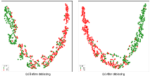
Figure 3: t-SNE feature visualization comparing the vanilla model (without debiasing) and the proposed debias model on right side. Red and Green points represent samples from two different classes of the BFFHQ dataset. After debiasing with the proposed model, noticeable enhancements in class discrimination are observed, resulting in better separation of classes and hence, better classification accuracy. (Best viewed in color).

6 Discussion and Future Work

CosFairNet introduces a novel network realignment method to reduce bias, especially when unbiased samples are scarce. This approach builds on the understanding that while low-level features learned in early network layers are not harmful, their spurious correlations with labels can be problematic. By employing an objective function within the parameter space, CosFairNet effectively uses the bias model to enrich these low-level features without creating unwanted correlations between features and labels. Despite its simplicity and efficacy, future work is needed.

Future directions include identifying which layers are most effective at learning various feature levels, a task complicated by differences in model architecture. For example, complex models may require several initial layers to learn low-level features effectively, whereas simpler datasets might only need the first layer. Another challenge arises when using pre-trained models where the weights are frozen, making it difficult to apply constraints in the parameter space. One potential solution is to introduce additional trainable layers before applying CosFairNet. Furthermore, while the method focuses on bias mitigation, it does not specifically address scenarios with multiple biases for a single class, presenting an opportunity for further exploration and enhancement of the model in handling a broader range of biases.

7 Conclusions

In this study, we introduce a novel bias mitigation method that addresses challenges encountered in prior approaches. Leveraging the insight that low-level features of biased samples are valuable for learning, our method focuses on mitigating unintended correlations between biased features and target labels. We utilize the bias model to enhance the learning of more effective and diverse low-level features while employing orthogonality constraints at later-stage layers. The proposed constraints in the parameter space ensure the preservation of low-level features while simultaneously preventing spurious correlations with target labels. Our approach is simple yet effective in mitigating bias and preventing its propagation through subsequent layers, offering a potential solution to some of the limitations of existing methods. In summary, this paper has shown that bias can be effectively curtailed by judiciously adjusting the model’s parameters. To tackle bias in machine learning models, our study highlights a novel direction and emphasizes the significance of incorporating diverse feature learning into the training process.

References

- [An et al.(2022)An, Kim, Ko, Lee, and Woo] Jaeju An, Taejune Kim, Donggeun Ko, Sangyup Lee, and Simon S Woo. A^ 2: Adaptive augmentation for effectively mitigating dataset bias. In Proceedings of the Asian Conference on Computer Vision, pages 4077–4092, 2022.
- [Arpit et al.(2017)Arpit, Jastrzkebski, Ballas, Krueger, Bengio, Kanwal, Maharaj, Fischer, Courville, Bengio, et al.] Devansh Arpit, Stanislaw Jastrzkebski, Nicolas Ballas, David Krueger, Emmanuel Bengio, Maxinder S Kanwal, Tegan Maharaj, Asja Fischer, Aaron Courville, Yoshua Bengio, et al. A closer look at memorization in deep networks. In International conference on machine learning, pages 233–242. PMLR, 2017.
- [Bahng et al.(2020)Bahng, Chun, Yun, Choo, and Oh] Hyojin Bahng, Sanghyuk Chun, Sangdoo Yun, Jaegul Choo, and Seong Joon Oh. Learning de-biased representations with biased representations. In International Conference on Machine Learning, pages 528–539. PMLR, 2020.
- [Bai et al.(2021)Bai, Sun, Hong, Zhou, Ye, Ye, Chan, and Li] Haoyue Bai, Rui Sun, Lanqing Hong, Fengwei Zhou, Nanyang Ye, Han-Jia Ye, S-H Gary Chan, and Zhenguo Li. Decaug: Out-of-distribution generalization via decomposed feature representation and semantic augmentation. In AAAI, 2021.
- [Barbano et al.(2023)Barbano, Dufumier, Tartaglione, Grangetto, and Gori] Carlo Alberto Barbano, Benoit Dufumier, Enzo Tartaglione, Marco Grangetto, and Pietro Gori. Unbiased supervised contrastive learning. In The Eleventh International Conference on Learning Representations, 2023. URL https://openreview.net/forum?id=Ph5cJSfD2XN.
- [Beery et al.(2018)Beery, Van Horn, and Perona] Sara Beery, Grant Van Horn, and Pietro Perona. Recognition in terra incognita. In Proceedings of the European conference on computer vision (ECCV), pages 456–473, 2018.
- [Dosovitskiy et al.(2014)Dosovitskiy, Springenberg, Riedmiller, and Brox] Alexey Dosovitskiy, Jost Tobias Springenberg, Martin Riedmiller, and Thomas Brox. Discriminative unsupervised feature learning with convolutional neural networks. Advances in neural information processing systems, 27, 2014.
- [Flachot and Gegenfurtner(2018)] Alban Flachot and Karl R Gegenfurtner. Processing of chromatic information in a deep convolutional neural network. JOSA A, 35(4):B334–B346, 2018.
- [Geirhos et al.(2018)Geirhos, Rubisch, Michaelis, Bethge, Wichmann, and Brendel] Robert Geirhos, Patricia Rubisch, Claudio Michaelis, Matthias Bethge, Felix A Wichmann, and Wieland Brendel. Imagenet-trained cnns are biased towards texture; increasing shape bias improves accuracy and robustness. arXiv preprint arXiv:1811.12231, 2018.
- [He et al.(2016)He, Zhang, Ren, and Sun] Kaiming He, Xiangyu Zhang, Shaoqing Ren, and Jian Sun. Deep residual learning for image recognition. In Proceedings of the IEEE conference on computer vision and pattern recognition, pages 770–778, 2016.
- [Hendrycks and Dietterich(2019)] Dan Hendrycks and Thomas Dietterich. Benchmarking neural network robustness to common corruptions and perturbations. arXiv preprint arXiv:1903.12261, 2019.
- [Hooker et al.(2020)Hooker, Moorosi, Clark, Bengio, and Denton] Sara Hooker, Nyalleng Moorosi, Gregory Clark, Samy Bengio, and Emily Denton. Characterising bias in compressed models. arXiv preprint arXiv:2010.03058, 2020.
- [Jeon et al.(2022)Jeon, Kim, Lee, Kang, and Lee] Myeongho Jeon, Daekyung Kim, Woochul Lee, Myungjoo Kang, and Joonseok Lee. A conservative approach for unbiased learning on unknown biases. In Proceedings of the IEEE/CVF Conference on Computer Vision and Pattern Recognition, pages 16752–16760, 2022.
- [K Kurmi et al.(2022)K Kurmi, Sharma, Sharma, and Namboodiri] Vinod K Kurmi, Rishabh Sharma, Yash Vardhan Sharma, and Vinay P. Namboodiri. Gradient based activations for accurate bias-free learning. In AAAI,, Feb 2022.
- [Kim et al.(2019)Kim, Kim, Kim, Kim, and Kim] Byungju Kim, Hyunwoo Kim, Kyungsu Kim, Sungjin Kim, and Junmo Kim. Learning not to learn: Training deep neural networks with biased data. In Proceedings of the IEEE/CVF Conference on Computer Vision and Pattern Recognition, pages 9012–9020, 2019.
- [Kim et al.(2021)Kim, Lee, and Choo] Eungyeup Kim, Jihyeon Lee, and Jaegul Choo. Biaswap: Removing dataset bias with bias-tailored swapping augmentation. In Proceedings of the IEEE/CVF International Conference on Computer Vision, pages 14992–15001, 2021.
- [Kim et al.(2022)Kim, Hwang, Ahn, Park, and Kwak] Nayeong Kim, Sehyun Hwang, Sungsoo Ahn, Jaesik Park, and Suha Kwak. Learning debiased classifier with biased committee. arXiv preprint arXiv:2206.10843, 2022.
- [Ko et al.(2023)Ko, Lee, Park, Noh, Park, and Kim] Donggeun Ko, Dongjun Lee, Namjun Park, Kyoungrae Noh, Hyeonjin Park, and Jaekwang Kim. Amplibias: Mitigating dataset bias through bias amplification in few-shot learning for generative models. In Proceedings of the 32nd ACM International Conference on Information and Knowledge Management, CIKM ’23, page 4028–4032, New York, NY, USA, 2023. Association for Computing Machinery. ISBN 9798400701245. 10.1145/3583780.3615184. URL https://doi.org/10.1145/3583780.3615184.
- [Krueger et al.(2021)Krueger, Caballero, Jacobsen, Zhang, Binas, Zhang, Le Priol, and Courville] David Krueger, Ethan Caballero, Joern-Henrik Jacobsen, Amy Zhang, Jonathan Binas, Dinghuai Zhang, Remi Le Priol, and Aaron Courville. Out-of-distribution generalization via risk extrapolation (rex). In International Conference on Machine Learning, pages 5815–5826. PMLR, 2021.
- [Lee et al.(2021)Lee, Kim, Lee, Lee, and Choo] Jungsoo Lee, Eungyeup Kim, Juyoung Lee, Jihyeon Lee, and Jaegul Choo. Learning debiased representation via disentangled feature augmentation. Advances in Neural Information Processing Systems, 34:25123–25133, 2021.
- [Lee et al.(2022)Lee, Park, Kim, Lee, Choi, and Choo] Jungsoo Lee, Jeonghoon Park, Daeyoung Kim, Juyoung Lee, Edward Choi, and Jaegul Choo. Revisiting the importance of amplifying bias for debiasing. AAAI-23, 5 2022. URL http://arxiv.org/abs/2205.14594.
- [Li and Vasconcelos(2019)] Yi Li and Nuno Vasconcelos. Repair: Removing representation bias by dataset resampling. In Proceedings of the IEEE/CVF conference on computer vision and pattern recognition, pages 9572–9581, 2019.
- [Li et al.(2023)Li, Evtimov, Gordo, Hazirbas, Hassner, Ferrer, Xu, and Ibrahim] Zhiheng Li, Ivan Evtimov, Albert Gordo, Caner Hazirbas, Tal Hassner, Cristian Canton Ferrer, Chenliang Xu, and Mark Ibrahim. A whac-a-mole dilemma: Shortcuts come in multiples where mitigating one amplifies others. In Proceedings of the IEEE/CVF Conference on Computer Vision and Pattern Recognition, pages 20071–20082, 2023.
- [Liu et al.(2023)Liu, Zhang, Sekhar, Wu, Singhal, and Fernandez-Granda] Sheng Liu, Xu Zhang, Nitesh Sekhar, Yue Wu, Prateek Singhal, and Carlos Fernandez-Granda. Avoiding spurious correlations via logit correction. In The Eleventh International Conference on Learning Representations, 2023. URL https://openreview.net/forum?id=5BaqCFVh5qL.
- [Mehrabi et al.(2021)Mehrabi, Morstatter, Saxena, Lerman, and Galstyan] Ninareh Mehrabi, Fred Morstatter, Nripsuta Saxena, Kristina Lerman, and Aram Galstyan. A survey on bias and fairness in machine learning. ACM computing surveys (CSUR), 54(6):1–35, 2021.
- [Nam et al.(2020)Nam, Cha, Ahn, Lee, and Shin] Junhyun Nam, Hyuntak Cha, Sungsoo Ahn, Jaeho Lee, and Jinwoo Shin. Learning from failure: De-biasing classifier from biased classifier. Advances in Neural Information Processing Systems, 33:20673–20684, 2020.
- [Park et al.(2023)Park, Lee, and Ye] Geon Yeong Park, Sang Wan Lee, and Jong Chul Ye. Efficient debiasing with contrastive weight pruning, 2023. URL https://openreview.net/forum?id=0DIkhwclYX3.
- [Qraitem et al.(2023)Qraitem, Saenko, and Plummer] Maan Qraitem, Kate Saenko, and Bryan A Plummer. Bias mimicking: A simple sampling approach for bias mitigation. In Proceedings of the IEEE/CVF Conference on Computer Vision and Pattern Recognition, pages 20311–20320, 2023.
- [Sagawa et al.(2019)Sagawa, Koh, Hashimoto, and Liang] Shiori Sagawa, PangWei Koh, Tatsunori B Hashimoto, and Percy Liang. Distributionally robust neural networks for group shifts: On the importance of regularization for worst-case generalization. arXiv preprint arXiv:1911.08731, 2019.
- [Selvaraju et al.(2017)Selvaraju, Cogswell, Das, Vedantam, Parikh, and Batra] Ramprasaath R Selvaraju, Michael Cogswell, Abhishek Das, Ramakrishna Vedantam, Devi Parikh, and Dhruv Batra. Grad-cam: Visual explanations from deep networks via gradient-based localization. In Proceedings of the IEEE international conference on computer vision, pages 618–626, 2017.
- [Tartaglione et al.(2021)Tartaglione, Barbano, and Grangetto] Enzo Tartaglione, Carlo Alberto Barbano, and Marco Grangetto. End: Entangling and disentangling deep representations for bias correction. In Proceedings of the IEEE/CVF conference on computer vision and pattern recognition, pages 13508–13517, 2021.
- [Teney et al.(2020)Teney, Abbasnejad, and van den Hengel] Damien Teney, Ehsan Abbasnejad, and Anton van den Hengel. Unshuffling data for improved generalization. arXiv preprint arXiv:2002.11894, 2020.
- [Torralba and Efros(2011)] Antonio Torralba and Alexei A. Efros. Unbiased look at dataset bias. In CVPR 2011, pages 1521–1528, 2011. 10.1109/CVPR.2011.5995347.
- [Vandenhirtz et al.(2023)Vandenhirtz, Manduchi, Marcinkevičs, and Vogt] Moritz Vandenhirtz, Laura Manduchi, Ričards Marcinkevičs, and Julia E Vogt. Signal is harder to learn than bias: Debiasing with focal loss. arXiv preprint arXiv:2305.19671, 2023.
- [Wang et al.(2019)Wang, He, Lipton, and Xing] Haohan Wang, Zexue He, Zachary C Lipton, and Eric P Xing. Learning robust representations by projecting superficial statistics out. arXiv preprint arXiv:1903.06256, 2019.
- [Wu et al.(2023)Wu, Yuksekgonul, Zhang, and Zou] Shirley Wu, Mert Yuksekgonul, Linjun Zhang, and James Zou. Discover and cure: Concept-aware mitigation of spurious correlation. In ICML, 2023.
- [Zhang and Sabuncu(2018)] Zhilu Zhang and Mert Sabuncu. Generalized cross entropy loss for training deep neural networks with noisy labels. Advances in neural information processing systems, 31, 2018.