DPVS-Shapley:Faster and Universal Contribution Evaluation Component in Federated Learning

Abstract.

In the current era of artificial intelligence, federated learning has emerged as a novel approach to addressing data privacy concerns inherent in centralized learning paradigms. This decentralized learning model not only mitigates the risk of data breaches but also enhances the system’s scalability and robustness. However, this approach introduces a new challenge: how to fairly and accurately assess the contribution of each participant. Developing an effective contribution evaluation mechanism is crucial for federated learning. Such a mechanism incentivizes participants to actively contribute their data and computational resources, thereby improving the overall performance of the federated learning system. By allocating resources and rewards based on the size of the contributions, it ensures that each participant receives fair treatment, fostering sustained engagement.Currently, Shapley value-based methods are widely used to evaluate participants’ contributions, with many researchers proposing modifications to adapt these methods to real-world scenarios. In this paper, we introduce a component called Dynamic Pruning Validation Set Shapley (DPVS-Shapley). This method accelerates the contribution assessment process by dynamically pruning the original dataset without compromising the evaluation’s accuracy. Furthermore, this component can assign different weights to various samples, thereby allowing clients capable of distinguishing difficult examples to receive higher contribution scores.

1. Introduction

Federated learningMcMahan et al. (2017) has emerged as a popular machine learning paradigm that allows for local data training, transmitting only model updates rather than raw data to a central server for aggregation. This approach ensures sensitive data remains within its domain, minimizing the risk of data breaches. While federated learning addresses issues such as data silos and privacy protection to some extent, a new challenge has arisen: how to fairly evaluate and compare the contributions of each client in a training session. Consequently, establishing a fair and effective incentive and reward allocation mechanism to encourage participants to provide higher quality data for circulation has become an urgent issue to resolve.

The Shapley valueShapley (1953) method has garnered significant attention from researchers due to its properties of group rationality, symmetry, null player, and additivity. However, it is also known for its high computational complexity and low efficiency. The evaluation process typically requires multiple rounds of validation on a validation set to accurately assess metrics such as accuracy. The original Shapley value approach, which required combining multi-party data and retraining the model, was extremely time-consuming. The introduction of MRSong et al. (2019) technology and gradient aggregation-based methods eliminated the need for iterative model retraining, significantly improving the time required for measuring contributions. Nevertheless, these methods still face the issue of exponential growth in validation iterations due to combinatorial calculations. Existing workGhorbani and Zou (2019)Liu et al. (2022)Jia et al. (2019b) primarily focuses on reducing the number of validation rounds through sampling and truncation techniques, thereby shortening the overall validation time. Additionally, gradient aggregation-based Shapley value methods assign equal weight to each sample in the validation set, which is evidently unreasonable as the value of test samples often varies.

To further enhance the efficiency of participant contribution assessment in Shapley value-based federated learning (FL), this paper proposes a method to accelerate the contribution evaluation process by reducing the time spent on each validation round, based on gradient aggregation techniques. We introduce the Dynamic Pruning Validation Set Shapley (DPVS-Shapley) method, which implements a dynamic pruning strategy on the validation set. By recording the results of the validation process, the validation set is divided into difficult and easy subsets. In each validation, extracting a certain proportion of cases from the easy subset and combining them with the difficult subset to form the validation set can achieve comparable accuracy to the full validation set while expediting the contribution assessment process. Furthermore, this method can assign different weights to the two types of samples, making the evaluation process more aligned with expectations and the assessment results more distinctive.

Our main contributions are as follows: 1) We have discovered that by eliminating a subset of samples from the validation set, we can still achieve performance approximating that of the original validation set. 2) We conducted ablation experiments to demonstrate the effectiveness of our regression strategy and its variations. 3) Extensive experiments under various FL data distribution settings (i.i.d. and non-i.i.d. data distributions) show that DPVS can effectively improve the efficiency of contribution calculations without compromising the contribution assessment.

2. Related Work

In recent years, the Shapley Value has also been widely applied in federated learning, primarily to assess the contribution of each participant to the training of the federated learning (FL) model.

The Shapley Value (SV) is a classical concept from game theory, introduced by Lloyd S. ShapleyShapley (1953) in 1953, to measure the contribution of each player to the total payoff in cooperative games.However, calculating the Shapley Value involves considering various possible coalition combinations and permutations. As the number of participants increases, the computational burden grows significantly. For a game with n participants, the computational complexity can reach $O(2^{n})$. To address this issue, Castro et al.Castro et al. (2009) proposed a Monte Carlo (MC) sampling method to approximate the Shapley Value with fewer utility evaluations, achieving favorable results. Following this, Maleki et al.Maleki et al. (2013) explored the complexity of approximating the Shapley Value (SV) using independent Monte Carlo methods, providing theoretical insights and proofs.Van Campen et al.van Campen et al. (2018)introduced the SMC-Shapley method, which first applied the Shapley Value framework to federated learning. They proposed a structured Monte Carlo sampling estimation method to effectively approximate the Shapley Value. Given the irregular utility values of different coalitions, their method approximates the Shapley Value by swapping participants’ positions within coalition sequences.Ghorbani et al. Ghorbani and Zou (2019) proposed the TMC-Shapley method, which calculates the Shapley Value for each data point by sequentially adding data points. At each addition, the algorithm computes the performance difference between the current and previous subsets. If the difference is below a pre-set performance tolerance threshold, the algorithm halts, thus achieving early termination and further reducing the computational load.Jia et al. Jia et al. (2019b) proposed the GTB-Shapley method. This method employs the concept of ”group testing,” where participants are divided into multiple groups for testing, thereby reducing the number of utility function evaluations.

Sampling-based methods effectively reduce the cost of the validation process. However, earlier approaches often require retraining the model, leading to significant time spent on repeated model training. Song et al. Song et al. (2019) proposed reconstructing the model based on gradients provided by participants, thereby avoiding model retraining and reducing the exponential cost.Jia et al.Jia et al. (2019a) introduced KNN-Shapley from a data pruning perspective, which employs K-nearest neighbors in federated tasks to perform data sample pruning for contribution assessment. However, this method exhibits considerable deviation compared to the true Shapley Value.Ghorbani et al. Ghorbani et al. (2020) explored scenarios with a large number of participants, where their method samples only a few participants to optimize the efficiency of contribution evaluation. The contributions of unsampled participants are then assessed using regression fitting.Liu et al. Liu et al. (2022) accelerated convergence and reduced computational costs by using guided permutation sampling combined with both inter-round and intra-round truncation.

Furthermore, some researchers have utilized utility function approximation methods to calculate contributions. Wang et al.Wang et al. (2020) proposed FedSV, which approximates the utility function by randomly selecting a group of clients, setting the contributions of other clients to zero in the current round. Fan et al.Fan et al. (2022b) introduced a novel contribution evaluation algorithm, ComFedSV, employing a low-rank matrix completion model to assess Shapley value-based contributions. This method records the improvement in the loss function between updated model parameters and those from the previous round. However, it is only applicable to horizontal federated learning. To address this limitation, Fan et al. subsequently proposed VerFedSVFan et al. (2022a) for vertical federated learning. This approach is suitable for both synchronous and asynchronous settings, evaluating data contributions while measuring communication and computational performance. Nevertheless, calculating Shapley values still requires considerable time. Other researchers have combined distributed computing, edge computing, homomorphic encryption, and other technologies with Shapley values. Ma et al.Ma et al. (2021) proposed a blockchain-based federated learning framework and a protocol for transparently evaluating each participant’s contribution. Liu et al.Liu et al. (2020) introduced a peer-to-peer payment system called FedCoin, utilizing a ”Proof of Shapley” (PoSap) consensus protocol to compute the Shapley value for each data owner, as opposed to traditional proof-of-work methods. Dong et al.Dong et al. (2023) presented an efficient Shapley value estimation method, leveraging the advantages of edge computing to achieve an affordable federated edge learning framework. Zheng et al.Zheng et al. (2022) proposed HESV, a homomorphic encryption-based single-server solution, and SecSV, a dual-server solution, to address security issues in federated learning systems.

3. Preliminaries

3.1. Shapley Value In Federated Learning

The Shapley Value (SV) is a classical concept from game theory, introduced by Lloyd S. ShapleyShapley (1953) in 1953, to measure the contribution of each player to the total payoff in cooperative games.

In federated learning, the Shapley Value is defined as follows: Consider $n$ participants with datasets $D_{1},D_{2},...,D_{n-1},D_{n}$,a model $M$,and a standard test set $T$.Let $D_{S}$ denote a combined dataset where $S\subseteq N$.The model $M$ trained on the dataset $D_{S}$ is denoted as $M_{S}$.The performance of the model on the standard test set is denoted by $U(M,T)$,abbreviated as $U(M)$.The Shapley Value $\phi(D_{N},T,D_{i})$,abbreviated as $\phi_{i}$, is used to compute the contribution of each FL participant $i$, and is defined by the formula:

$$\phi_{i}=C\sum_{S\subseteq N\setminus\{i\}}\frac{U(M_{S\bigcup\{i\}})-U(M_{S})}{\dbinom{n-1}{|S|}}$$

Where C is a constant. Obviously, calculating Shapley requires a lot of retraining of the model, which creates a huge overhead, which is unacceptable for individual clients.

3.2. Optimization Strategies

Before computing Shapley values based on model aggregation, obtaining model performance metrics often requires retraining the models. This can lead to significant time spent on training models based on different data combinations, which is clearly unacceptable for participants, as they do not gain additional rewards from the evaluation process. The proposals of MRSong et al. (2019) address this issue by accumulating the contribution of each new round of evaluation and using the model, which aggregates client gradients, as the new base model, thus solving the problem of model retraining. This shift moves the primary time-consuming part of contribution evaluation from model training to model evaluation.

Currently, most methods rely on samplingWang et al. (2019) and early stopping to achieve the convergence of the convergence function and ultimately fit the true Shapley values. These methods primarily aim to accelerate by reducing the number of validations on the validation set. From another perspective, acceleration can also be achieved by attempting to reduce the time of each individual validation, which aligns with the concept of data pruning. By reducing the amount of data that needs to be validated, corresponding speed improvements can be achieved. Based on local correlation characteristics, federated learning uses K-nearest neighbor task models to achieve data sample pruning for contribution evaluationJia et al. (2019a).

3.3. Model Stability

Support Vector Machine (SVM)Jakkula (2006)Yu and Kim (2012) is a machine learning algorithm used for classification and regression analysis, with its primary application in classification problems. The core concept of SVM is to identify an optimal decision boundary (hyperplane) that separates data points into different categories while maximizing the margin between classes. As the learning process progresses, changes in the classification boundary become increasingly subtle, with most samples consistently remaining on one side of the hyperplane. Points closer to the decision boundary have a higher likelihood of being classified to the opposite side in the next round of model training. During the validation process, we tend to focus more on the points that are misclassified in the current round and those that are likely to be misclassified in the next, while paying relatively less attention to the points that are stably classified on either side.

The universal approximation capability of neural networks was demonstrated by Cybenko et al.Cybenko (1989), showing that single-hidden-layer neural networks can approximate any continuous function. Hornik et al.Hornik et al. (1989) further explored the universal approximation capabilities of multi-layer feedforward neural networks, explaining why neural networks can learn complex decision boundaries. Neural networks leverage their hierarchical structure and non-linear activation functions to learn highly complex decision boundaries, enabling sophisticated mappings from input to output.

Although the decision boundaries of neural networks are often highly non-linear, sample classification tends to stabilize as the model is trained. We have adapted our SVM-inspired approach to neural networks, considering samples that are consistently classified correctly and far from the decision boundary as candidates for pruning. This approach allows us to progressively reduce the number of samples being tested.

4. The Proposed Approach

4.1. Main Process

Based on the existing problems and related explorations, we propose a method for validation set pruning aimed at accelerating the single-round validation process by reducing the number of validation samples, thereby speeding up the entire contribution assessment process. Figure 1 illustrates the confidence regression-based flowchart. In federated learning, the server distributes the model, and clients upload gradients to the server after local training. Contribution assessment methods based on gradient combination using Shapley value require repeatedly combining gradients and evaluating on a validation set. The final contribution proportions are then calculated based on marginal benefits derived from all validation results.

Our method comprises two phases.The first phase is the experience accumulation phase, during which no pruning is performed on the validation set. This is because the model is still relatively unstable at this stage and unable to effectively distinguish between simple and difficult examples. By evaluating the model on the complete validation set, we accumulate multiple rounds of sample decision results and decision confidence scores. Once the accumulated quantity meets the requirements, we can classify the samples into simple and difficult examples, allowing us to enter the dynamic pruning phase.

The second phase is the dynamic pruning phase. In this stage, we first categorize the samples in the validation set into difficult and simple examples based on previous sample judgment results. According to our extraction strategy, we select a corresponding proportion of simple examples and combine them with all difficult examples to obtain the pruned test set. If a confidence-based extraction strategy is chosen, the probability of selecting samples with lower confidence increases during the extraction process. We believe that these samples are closer to the decision boundary, and their judgment results are more likely to change in the model’s next training process.The pruning algorithm is shown in Algorithm 1.

We run the aggregated model on this dynamically pruned validation set to obtain the model’s accuracy on the pruned test set and collect intermediate results. Since our accuracy does not include the pruned samples, we need to adjust this accuracy accordingly. The final accuracy formula 1 is shown as follows.

$$\begin{split}Acc_{final}={(100*\frac{N_{prune}}{N_{sum}}+Acc_{dynamic}*\frac{N_{dynamic}}{N_{sum}})}\end{split}$$ (1)

As the results collected during the validation process only include unpruned test samples, we need to supplement the validation results and confidence scores of the pruned data using historical records. For the judgment results of pruned samples, we assume all are correct by default. However, for confidence scores, we apply a certain confidence decay, because as the model training rounds accumulate, doubts arise about previous classification results. Reducing confidence increases the probability of the sample being selected in the next extraction, thereby enabling timely and effective regression. The regression algorithm is shown in Algorithm 2.

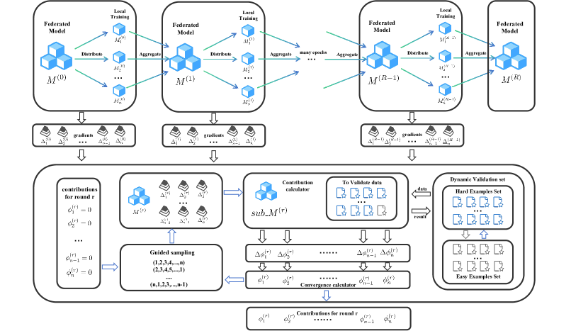
Figure 1. DVPS-Shapely

Input: numEpoch, startDynamicEpoch, sampleRate, n, m, judgeResultMatrix, judgeConfidenceMatrix, allValidationCases, randomType

Output: needValidationCases

1 if nowEpoch $<$ startDynamicEpoch then

2       return allValidationCases;

3      

4else

5       foreach valCase $\in$ allValidationCases do

6             if valCase latest n epoch is all correct in judgeResultMatrix then

7                   add valCase to easySet;

8                  

9            else

10                   add valCase to hardSet;

11                  

12            

13      if randomType $==$ None then

14             return easySet;

15            

16       else if randomType $==$ Random then

17             selectSet $\leftarrow$ randomly select n percent of the samples from the easySet;

18             return selectSet $\cup$ hardSet;

19            

20       else if randomType $==$ WeightRandom then

21             weights $\leftarrow$ [];

22             foreach easyCase $\in$ easySet do

23                   aveConfidence $\leftarrow$ average the confidence level of the last m rounds of this easyCase;

24                   add aveConfidence to weights;

25                  

26            selectSet $\leftarrow$ randomly select n percent of the samples from the easySet based on weights;

27             return selectSet $\cup$ hardSet;

28            

29      

Algorithm 1 Dynamic pruning algorithm

Input: numEpoch, startDynamicEpoch, judgeResultRecord, judgeResultMatrix, confidenceResultRecord, confidenceResultMatrix, beta

Output: judgeResultMatrix, confidenceResultMatrix

1

2if nowEpoch $<$ startDynamicEpoch then

3       add judgeResultRecord to judgeResultMatrix;

4       add confidenceResultRecord to confidenceResultMatrix;

5       return ;

6      

7allJudgetRecord $\leftarrow$ [];

8 allConfRecord $\leftarrow$ confidenceResultMatrix[-1];

9 for i $\leftarrow$ 0 to testCaseNum - 1 do

10       if judgeResultRecord contains the result of the i-th sample then

11             allJudgetRecord[i] $\leftarrow$ judgeResultRecord[i];

12            

13      else

14             allJudgetRecord[i] $\leftarrow$ 1;

15            

16      if confidenceResultRecord contains the confidence of the i-th sample then

17             allConfRecord[i] $\leftarrow$ confidenceResultRecord[i];

18            

19      else

20             allConfRecord[i] $\leftarrow$ allConfRecord[i] $\times$ beta;

21            

22      

23add allJudgetRecord to judgeResultMatrix;

24 add allConfRecord to confidenceResultMatrix;

25 return ;

Algorithm 2 Information updating algorithm

4.2. Why and how to prune simple sample

To further reduce the time spent on contribution evaluation, we propose the concept of Dynamic Pruned Validation Set (DPVS) from the perspective of decreasing the validation time per round. The question of which examples to include in the pruned dataset arises. We posit that samples that do not affect accuracy should be eliminated, specifically those consistently classified correctly during the model’s decision process. Such samples have negligible impact on accuracy, as we can largely anticipate their correct classification in the subsequent validation round. To further reduce the time consumed by contribution assessment, we propose the concept of Dynamic Pruning Validation Set (DPVS) from the perspective of decreasing validation time per round. The question of which examples in the pruned dataset to retain becomes a new challenge. We argue that samples that do not affect accuracy should be removed, specifically those consistently classified correctly during the model’s discrimination process. Such examples have minimal impact on accuracy, as we can largely anticipate their correct classification in subsequent validation rounds. We define these as simple samples. To this end, we collect the classification results for each round, $R_{sample}=[0,1,1,....,1,0,1]$, which indicates whether each sample was correctly classified. After n rounds, we obtain a two-dimensional matrix containing the validation results. This matrix allows us to categorize the validation set samples into simple and difficult samples. We define simple samples as follows: if a sample is correctly classified in all of the most recent n rounds, it is considered an simple sample; otherwise, it is deemed a difficult sample. In our subsequent experiment, ”Simple sample scale in different dataset”, we found that the proportion of simple samples varies from approximately 30%+ to 90%+ across different datasets. This finding suggests that our categorization is meaningful and can potentially achieve corresponding proportions of validation acceleration. By focusing solely on predicting difficult samples, we can achieve faster validation speeds. However, considering that models undergo continuous changes during the training process, which may lead to previously simple samples becoming misclassified, it is necessary to consider how to timely and effectively reintegrate these samples into the validation set.

4.3. Strategies for Updating Dynamically Pruned Validation Sets

To address this issue, we propose two methods: random regression and confidence-based regression. Random regression involves randomly selecting a certain proportion of samples from the simple samples to combine with the difficult examples, forming the validation set. Each simple sample has an equal probability of being selected, while the remaining simple samples constitute the pruned portion. The confidence-based regression method requires collecting not only the classification results but also the confidence levels associated with these results. We apply a function transformation to the confidence levels, ensuring that simple samples with higher confidence have a lower probability of being selected during the sampling process.

To address different objectives, we propose two update timing strategies. The EE strategy aims to update the validation set after each validation round, ensuring that the accuracy obtained from this set more closely approximates the true accuracy. However, in our subsequent experiment ”Effect of aggregated gradient number on the accuracy of pruning data set”, we discovered that when the number of combined gradients is low, the resulting aggregated model becomes too similar to a single client’s model. This leads to significant discrepancies in accuracy. Consequently, we found it necessary to increase the sampling ratio when dealing with a smaller number of combined gradients.To assign greater importance to difficult samples and further accelerate contribution measurement, we propose the ET strategy. This strategy updates the validation set only before contribution calculation, ensuring that all gradient-combined models are validated on the same set. By adopting this strategy, we no longer focus on fitting the contribution of the original Multi-Round (MR) approach, allowing us to use a smaller regression ratio. The purpose of this strategy is to widen the gap between different parties’ contributions, enabling clients capable of identifying difficult samples to have a larger contribution share. This approach increases the disparity between parties, enhancing differentiation and facilitating effective contribution ranking.

5. Experimental Evaluation

5.1. Settings

The hardware and software environments for the experiment are as follows:

• Operating system: Ubuntu 16

• Development language: Python 3.9

• CPU: Intel Xeon Gold 5118

• GPU: NVIDIA RTX A4000, 16GB of video memory.

• Memory: 96GB

• Hard disk: 3.6TB capacity

This experiment employs the FedAvg (Federated Averaging) strategy for federated aggregation. The dataset used in the experiments is CIFAR-10, with five primary data configurations:

• SDSS: Clients have the same distribution of the same size data.

• DDSS: Clients with different distributions of data of the same size.

• SDDS: Clients with the same distribution of data of different size.

• NFSS: Clients have data of the same size from the same distribution, but there is some noise in the client’s features.

• NLSS: Clients have data of the same size from the same distribution, but there is some noise in the client’s labeling.

Table 1. Experiments Setting

Dataset	Data Type	Model
IrisFisher (1936)	Value	MLP
CIFAR-10Krizhevsky et al. (2009), MNISTLeCun et al. (1998),          FASHION-MNISTXiao (2017)	Image	ResNet18
Movie Review DatasetMaas et al. (2011)	Text	LSTM

5.2. Simple sample scale in different dataset

To validate the proportional scale of simple examples across various types of datasets, we trained corresponding models on numerical, image, and text datasets, recording the results of each validation round. In this experiment, we employed a single-machine training mode and split the dataset into training and testing sets with an 8:2 ratio. The criterion for identifying simple examples was as follows: samples correctly classified for 30 consecutive training epochs were designated as simple examples. The remaining experimental settings are detailed in table1

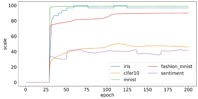
Figure 2. Simple sample scale in different dataset

As shown in Figure 2, the experimental results demonstrate significant variations in the proportion of simple examples across different types and categories of datasets. Generally, this proportion ranges from 30%+ to 90%+, indicating that pruning the validation set is indeed meaningful and potentially beneficial.

5.3. Time comparison of different strategies

We have performed model training on the cifar-10 dataset after putting our strategy on the cifar-10 dataset with different strategies. The experimental results are shown in the following figure3.The time per round of validation for our method in the early time is higher than the original full time, but as the accuracy of the model increases, the number of pruned samples increases, which offsets this consumption and saves more time. It can be seen that the overall picture is that the Ignore strategy drops the fastest in the time dimension. Since randomChoose will have a portion of regression, resulting in the consumption of time to process the random strategy and the testing of this portion of regression samples, randomChoose will be higher than the Ignore strategy. Since weightChoose has to perform weight randomization compared to randomChoose, this operation will consume more time compared to randomChoose.Concurrently, under the same number of rounds, the weightChoose pruning method eliminates fewer data points compared to randomChoose. This is because weightChoose demonstrates a superior ability to accurately identify samples that transition from being simple to challenging examples due to model modifications.

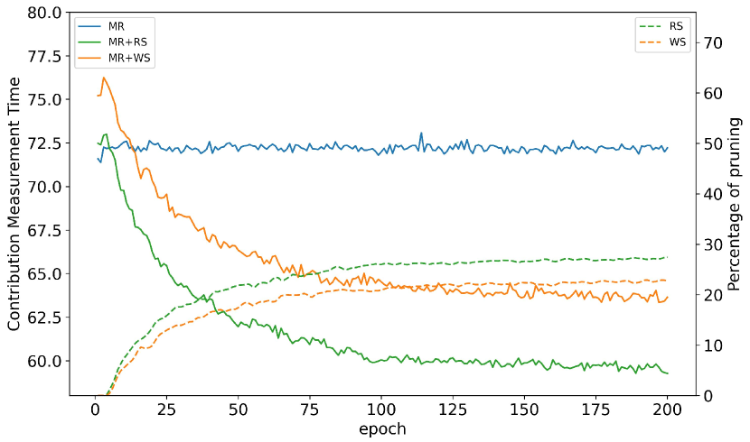
Figure 3. Evalution change under different strategies

5.4. Effect of aggregated gradient number on the accuracy of pruning data set

To validate the accuracy of our method on federated learning, we average the cifar-10 data across 5 clients and validate it on the server. Since gradient combinations are needed to compute the sum of marginal effects across clients, we perform a difference measure between real and simulated accuracy for various length combinations. For this purpose, we set up controlled experiments to demonstrate the effectiveness of weighted sampling (WS) and the sampling proportion determined by the number of clients (CNDSR) in our method. For the RS and WS experiments we chose a regression proportion of 0.05 from the pruned sample. for CNDSR the aggregated number of clients 1,2,3,4,5, the regression proportions were taken to be 0.5,0.4,0.3,0.2,0.1 respectively.

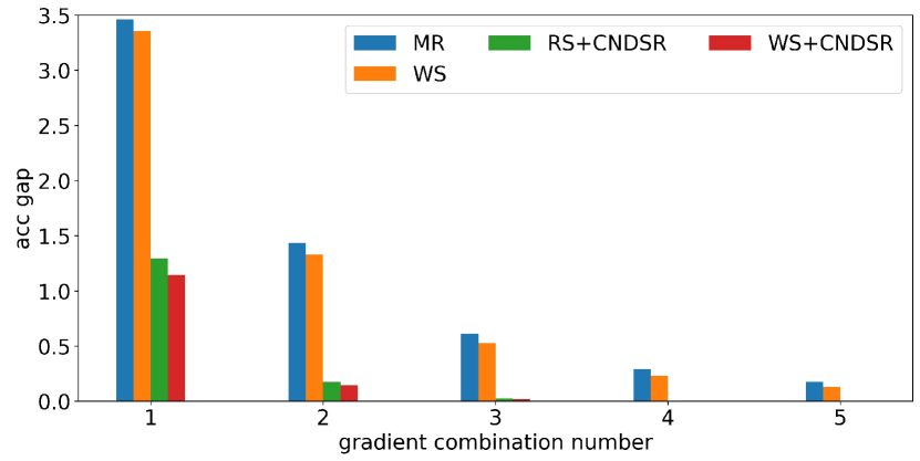
Figure 4. Gap between fitted accuracy and true accuracy

The experimental results indicate that an insufficient number of combinations can cause the model parameters to excessively align with a single client’s local data, leading to over-localization. This prevents the model from learning global features, resulting in significant model fluctuations and a substantial disparity between the fitted accuracy and the true accuracy, potentially impacting the contribution assessment results. When employing the CNDSR-based method, we observed that moderately increasing the proportion of samples helps reduce the accuracy gap. Similarly, the WS method also contributes to narrowing this discrepancy. With 3-5 clients, the CNDSR-based method achieves accuracy nearly identical to the true values. Consequently, when aggregating data from a small number of clients, we extract a larger proportion of samples, or even all samples, from the redundant dataset.

5.5. Tested on gradient aggregation-based MR

Finally we applied our components on the Shapley value method based on gradient aggregation and simulated five data distribution conditions to verify the effectiveness of our method,and the five data settings are as above.

We adopt the gradient aggregation-based method MR, which is the earliest approach to calculate Shapley values for measuring participant contributions through gradient aggregation. Many subsequent methods have built upon and improved this approach. The main concept of this method is as follows: In each round, the server collects gradient updates from clients. By combining these gradients, relevant sub-models are reconstructed, and performance metrics are evaluated on these sub-models. Finally, the contribution of each party is determined by summing the marginal benefits across different combinations.

Evaluation Metrics.We compare different methods on the following metrics.

• Time Saving: Calculate the percentage of time saved by each party’s contribution.

• Cosine Distance: Let the vectors of normalized contribution index of different data providers calculated according to the True Shapley and by an approximated method is denoted by $\phi^{*}=\langle\phi_{1}^{*},\phi_{2}^{*},\cdots,\phi_{n}^{*}\rangle\quad\text{and}\quad\phi=\langle\phi_{1},\phi_{2},\cdots,\phi_{n}\rangle$, respectively. The Cosine Distance is defined by

  $$d_{\text{cos}}(\phi^{*},\phi)=1-\frac{\sum_{i=1}^{n}\phi_{i}^{*}\cdot\phi_{i}}{\sqrt{\sum_{i=1}^{n}(\phi_{i}^{*})^{2}}\sqrt{\sum_{i=1}^{n}(\phi_{i})^{2}}}$$

• Euclidean Distance: The Euclidean Distance is defined by

  $$d_{\text{euclid}}(\phi^{*},\phi)=\sqrt{\sum_{i=1}^{n}(\phi_{i}^{*}-\phi_{i})^{2}}$$

• Maximum Difference: The Maximum Difference is defined by

  $$d_{\text{max}}(\phi^{*},\phi)=\max_{1\leq i\leq n}|\phi_{i}^{*}-\phi_{i}|$$

The other settings of the experiment were as follows:

• RD:Random sample from easy set.

• WR:Random selection by weight from easy set.

• [1.0,1.0,0.5,0.1,0.1]is the extraction ratios for different length combinations in EE.

• [0.1,0.1,0.1,0.1,0.1]is the extraction ratios for different length combinations in ET.

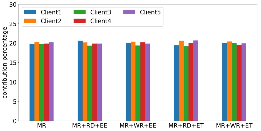
Figure 5. Contributions under sdss

Figure 6. Contributions under sdds

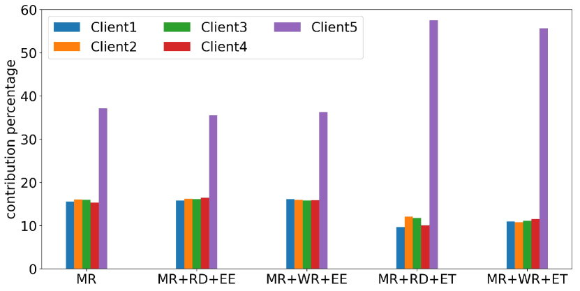
Figure 7. Contributions under ddss

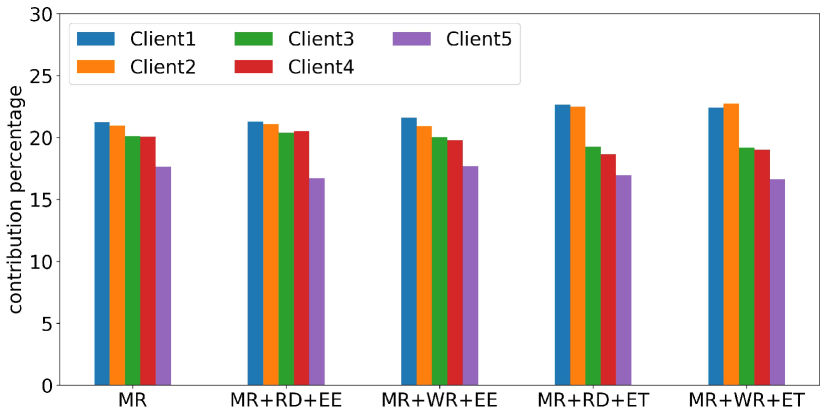
Figure 8. Contributions under nfss

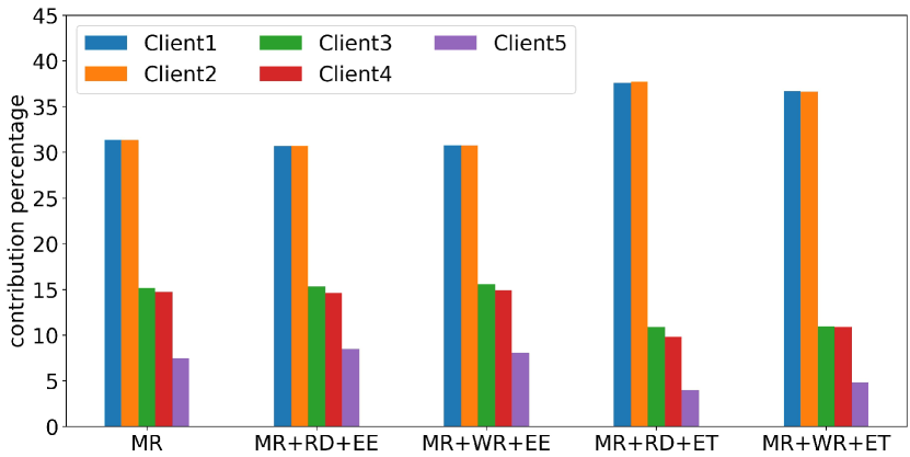
Figure 9. Contributions under nlss

Table 2. Metrics under SDSS

	Time Saving	Cosine Distance	Euclidean Distance	Maximum Difference
MR+RD+EE	10.47591	0.000210	0.916187	0.760000
MR+WR+EE	9.78873	0.000102	0.637495	0.359999
MR+RD+ET	34.09605	0.000219	0.937389	0.570000
MR+WR+ET	32.20264	0.000079	0.565066	0.339999

Table 3. Metrics under DDSS

	Time Saving	Cosine Distance	Euclidean Distance	Maximum Difference
MR+RD+EE	12.40040	0.000750	1.995294	1.630000
MR+WR+EE	7.51847	0.000270	1.192308	0.890000
MR+RD+ET	28.58902	0.057952	22.649048	20.40000
MR+WR+ET	26.78545	0.051820	20.689838	18.47999

Table 4. Metrics under SDDS

	Time Saving	Cosine Distance	Euclidean Distance	Maximum Difference
MR+RD+EE	12.51104	0.000121	0.702139	0.500000
MR+WR+EE	11.84869	0.000026	0.330151	0.199999
MR+RD+ET	31.24816	0.023610	10.329632	8.579999
MR+WR+ET	27.17839	0.018510	9.076012	7.770000

Table 5. Metrics under NFSS

	Time Saving	Cosine Distance	Euclidean Distance	Maximum Difference
MR+RD+EE	12.68942	0.000278	1.060188	0.910000
MR+WR+EE	7.24584	0.000055	0.472652	0.349999
MR+RD+ET	33.20582	0.001881	2.760706	1.529999
MR+WR+ET	25.24643	0.001841	2.733148	1.779999

Table 6. Metrics under NLSS

	Time Saving	Cosine Distance	Euclidean Distance	Maximum Difference
MR+RD+EE	10.61531	0.000314	1.387372	1.010000
MR+WR+EE	6.10894	0.000219	1.137365	0.600000
MR+RD+ET	30.14041	0.018381	11.567329	6.399999
MR+WR+ET	24.26670	0.013626	9.746902	5.309999

In the EE experiments, we aimed to closely match the performance of the MR method. As evidenced by the data in Tables 2-6 and Figures 5-9, our method achieves nearly identical fitting results compared to the original MR method. This observation is further corroborated by various metrics including Cosine Distance, Euclidean Distance, and Maximum Difference. Notably, we achieved a 9% to 14% improvement in speed, as indicated by the Time Saving metric.The success of our method in accurately simulating the original dataset’s accuracy can be attributed to two key strategies: timely updates and setting higher sampling ratios for fewer combinations. These findings not only validate our experimental hypothesis but also demonstrate that the MR method can achieve speed improvements within an acceptable margin of error.

When shifting our focus from replicating the MR method to assigning higher weights to difficult samples, the ET strategy becomes a preferable choice. The ET strategy amplifies the disparities in contributions among parties, enabling a more distinct tiered ranking of contributions for stakeholders primarily concerned with contribution rankings. Consider the nfss data configuration illustrated in Figure 8: Clients 1 and 2 have unaltered data features, Clients 3 and 4 have 15% Gaussian noise added to their data, and Client 5 has 30% noise added. In this scenario, the conventional MR method struggles to clearly differentiate between Clients 1, 2 and Clients 3, 4 due to their closely aligned contribution values. This similarity makes it challenging to definitively assert that the data quality of Clients 1 and 2 is superior to that of Clients 3 and 4, especially considering the inherent randomness in model training processes. By employing the ET strategy, we set lower regression ratios across different combinations, resulting in a pruned dataset with a higher proportion of difficult samples, thereby increasing the weight of these challenging examples. This approach successfully widens the gap in contribution percentages among parties with varying data quality during the testing phase, leading to a more effective contribution ranking. Moreover, this method significantly enhances the speed of contribution assessment, achieving an acceleration effect of over 30%+.

6. Conclusion

This paper addresses the challenge of enhancing contribution assessment efficiency in federated learning (FL) systems. We introduce the Dynamic Validation Pruning Set Shapley (DPVS-Shapley) method, which employs a dynamic pruning strategy to categorize the validation set into simple and difficult samples. By selectively regressing different proportions of simple samples, we achieve two objectives: reducing overall validation time without compromising accuracy, and amplifying the contribution disparities among parties by assigning higher weights to difficult samples while significantly shortening validation time.

If you wish to include any acknowledgments in your paper (e.g., to people or funding agencies), please do so using the ‘acks’ environment. Note that the text of your acknowledgments will be omitted if you compile your document with the ‘anonymous’ option.

References

- (1)
- Castro et al. (2009) Javier Castro, Daniel Gómez, and Juan Tejada. 2009. Polynomial calculation of the Shapley value based on sampling. Computers & operations research 36, 5 (2009), 1726–1730.
- Cybenko (1989) George Cybenko. 1989. Approximation by superpositions of a sigmoidal function. Mathematics of control, signals and systems 2, 4 (1989), 303–314.
- Dong et al. (2023) Liguo Dong, Zhenmou Liu, Kejia Zhang, Abdulsalam Yassine, and M Shamim Hossain. 2023. Affordable federated edge learning framework via efficient Shapley value estimation. Future Generation Computer Systems 147 (2023), 339–349.
- Fan et al. (2022b) Zhenan Fan, Huang Fang, Zirui Zhou, Jian Pei, Michael P Friedlander, Changxin Liu, and Yong Zhang. 2022b. Improving fairness for data valuation in horizontal federated learning. In 2022 IEEE 38th International Conference on Data Engineering (ICDE). IEEE, 2440–2453.
- Fan et al. (2022a) Zhenan Fan, Huang Fang, Zirui Zhou, Jian Pei, Michael P Friedlander, and Yong Zhang. 2022a. Fair and efficient contribution valuation for vertical federated learning. arXiv preprint arXiv:2201.02658 (2022).
- Fisher (1936) Ronald A Fisher. 1936. The use of multiple measurements in taxonomic problems. Annals of eugenics 7, 2 (1936), 179–188.
- Ghorbani et al. (2020) Amirata Ghorbani, Michael Kim, and James Zou. 2020. A distributional framework for data valuation. In International Conference on Machine Learning. PMLR, 3535–3544.
- Ghorbani and Zou (2019) Amirata Ghorbani and James Zou. 2019. Data shapley: Equitable valuation of data for machine learning. In International conference on machine learning. PMLR, 2242–2251.
- Hornik et al. (1989) Kurt Hornik, Maxwell Stinchcombe, and Halbert White. 1989. Multilayer feedforward networks are universal approximators. Neural networks 2, 5 (1989), 359–366.
- Jakkula (2006) Vikramaditya Jakkula. 2006. Tutorial on support vector machine (svm). School of EECS, Washington State University 37, 2.5 (2006), 3.
- Jia et al. (2019a) Ruoxi Jia, David Dao, Boxin Wang, Frances Ann Hubis, Nezihe Merve Gurel, Bo Li, Ce Zhang, Costas J Spanos, and Dawn Song. 2019a. Efficient task-specific data valuation for nearest neighbor algorithms. arXiv preprint arXiv:1908.08619 (2019).
- Jia et al. (2019b) Ruoxi Jia, David Dao, Boxin Wang, Frances Ann Hubis, Nick Hynes, Nezihe Merve Gürel, Bo Li, Ce Zhang, Dawn Song, and Costas J Spanos. 2019b. Towards efficient data valuation based on the shapley value. In The 22nd International Conference on Artificial Intelligence and Statistics. PMLR, 1167–1176.
- Krizhevsky et al. (2009) Alex Krizhevsky, Geoffrey Hinton, et al. 2009. Learning multiple layers of features from tiny images. (2009).
- LeCun et al. (1998) Yann LeCun, Léon Bottou, Yoshua Bengio, and Patrick Haffner. 1998. Gradient-based learning applied to document recognition. Proc. IEEE 86, 11 (1998), 2278–2324.
- Liu et al. (2020) Yuan Liu, Zhengpeng Ai, Shuai Sun, Shuangfeng Zhang, Zelei Liu, and Han Yu. 2020. Fedcoin: A peer-to-peer payment system for federated learning. In Federated learning: privacy and incentive. Springer, 125–138.
- Liu et al. (2022) Zelei Liu, Yuanyuan Chen, Han Yu, Yang Liu, and Lizhen Cui. 2022. Gtg-shapley: Efficient and accurate participant contribution evaluation in federated learning. ACM Transactions on intelligent Systems and Technology (TIST) 13, 4 (2022), 1–21.
- Ma et al. (2021) Shuaicheng Ma, Yang Cao, and Li Xiong. 2021. Transparent contribution evaluation for secure federated learning on blockchain. In 2021 IEEE 37th international conference on data engineering workshops (ICDEW). IEEE, 88–91.
- Maas et al. (2011) Andrew L. Maas, Raymond E. Daly, Peter T. Pham, Dan Huang, Andrew Y. Ng, and Christopher Potts. 2011. Learning Word Vectors for Sentiment Analysis. In Proceedings of the 49th Annual Meeting of the Association for Computational Linguistics: Human Language Technologies. Association for Computational Linguistics, Portland, Oregon, USA, 142–150. http://www.aclweb.org/anthology/P11-1015
- Maleki et al. (2013) Sasan Maleki, Long Tran-Thanh, Greg Hines, Talal Rahwan, and Alex Rogers. 2013. Bounding the estimation error of sampling-based Shapley value approximation. arXiv preprint arXiv:1306.4265 (2013).
- McMahan et al. (2017) Brendan McMahan, Eider Moore, Daniel Ramage, Seth Hampson, and Blaise Aguera y Arcas. 2017. Communication-efficient learning of deep networks from decentralized data. In Artificial intelligence and statistics. PMLR, 1273–1282.
- Shapley (1953) L. S. Shapley. 1953. A value for n-person games. Annals of Mathematical Studies (1953), 307–317.
- Song et al. (2019) Tianshu Song, Yongxin Tong, and Shuyue Wei. 2019. Profit allocation for federated learning. In 2019 IEEE International Conference on Big Data (Big Data). IEEE, 2577–2586.
- van Campen et al. (2018) Tjeerd van Campen, Herbert Hamers, Bart Husslage, and Roy Lindelauf. 2018. A new approximation method for the Shapley value applied to the WTC 9/11 terrorist attack. Social Network Analysis and Mining 8 (2018), 1–12.
- Wang et al. (2019) Guan Wang, Charlie Xiaoqian Dang, and Ziye Zhou. 2019. Measure contribution of participants in federated learning. In 2019 IEEE international conference on big data (Big Data). IEEE, 2597–2604.
- Wang et al. (2020) Tianhao Wang, Johannes Rausch, Ce Zhang, Ruoxi Jia, and Dawn Song. 2020. A principled approach to data valuation for federated learning. Federated Learning: Privacy and Incentive (2020), 153–167.
- Xiao (2017) H Xiao. 2017. Fashion-mnist: a novel image dataset for benchmarking machine learning algorithms. arXiv preprint arXiv:1708.07747 (2017).
- Yu and Kim (2012) Hwanjo Yu and Sungchul Kim. 2012. SVM Tutorial-Classification, Regression and Ranking. Handbook of Natural computing 1 (2012), 479–506.
- Zheng et al. (2022) Shuyuan Zheng, Yang Cao, and Masatoshi Yoshikawa. 2022. Secure Shapley Value for Cross-Silo Federated Learning (Technical Report). arXiv preprint arXiv:2209.04856 (2022).