Out-of-distribution Robust Optimization

Zhongze Cai, Hansheng Jiang, Xiaocheng Li
(Imperial College Business School, Imperial College London, (z.cai22, xiaocheng.li)@imperial.ac.uk
Rotman School of Management, University of Toronto, hansheng.jiang@rotman.utoronto.ca
)
Abstract

In this paper, we consider the contextual robust optimization problem under an out-of-distribution setting. The contextual robust optimization problem considers a risk-sensitive objective function for an optimization problem with the presence of a context vector (also known as covariates or side information) capturing related information. While the existing works mainly consider the in-distribution setting, and the resultant robustness achieved is in an out-of-sample sense, our paper studies an out-of-distribution setting where there can be a difference between the test environment and the training environment where the data are collected. We propose methods that handle this out-of-distribution setting, and the key relies on a density ratio estimation for the distribution shift. We show that additional structures such as covariate shift and label shift are not only helpful in defending distribution shift but also necessary in avoiding non-trivial solutions compared to other principled methods such as distributionally robust optimization. We also illustrate how the covariates can be useful in this procedure. Numerical experiments generate more intuitions and demonstrate that the proposed methods can help avoid over-conservative solutions.

1 Introduction

Contextual optimization considers a constrained optimization problem with the presence of covariates (context), and it can be viewed as a prediction problem under an optimization context where the output of the prediction model serves as the objective function for the downstream optimization problem. The goal is to develop a model (trained from past data) that prescribes a decision/solution for the downstream optimization problem using the covariates directly but without observation of the objective function. It has been extensively studied in recent years under various settings (Hu et al., 2022; Elmachtoub and Grigas, 2022; Bertsimas and Kallus, 2020; Ho-Nguyen and Kılınç-Karzan, 2022; Chen and Kılınç-Karzan, 2020; Wilder et al., 2019; Sun et al., 2023b; Huang and Gupta, 2024), and we refer to Sadana et al. (2024) for a survey on the topic. In this paper, we consider the problem of contextual robust optimization where the objective function of the optimization problem becomes a risk-sensitive one. Unlike all existing works, we consider a distribution shift/out-of-distribution setting where the test environment is different from the training environment that generates the training dataset. In this sense, the notion of robustness goes beyond the existing scope and it also covers robustness against the distribution shift. To summarize, our contributions are as follows:

First, we formulate the problem of out-of-distribution robust optimization and propose a method that utilizes a density ratio estimate to make inferences about the test environment with data from the training environment.

Second, we derive theoretical guarantees for the proposed method and use an analytical example to illustrate the values of shift structure in avoiding over-conservative solutions.

Third, we conduct numerical experiments to generate more intuitions for the setup and illustrate the effectiveness of the proposed method.

Related Literature. The study of robust optimization has a long history which considers risk-sensitive objectives and approximate solutions using the notion of uncertainty set (see Ghaoui et al. (2003); Chen et al. (2007); Natarajan et al. (2008) among others). A recent line of works considers the contextual formulation for robust optimization Chenreddy et al. (2022); Sun et al. (2023a); Patel et al. (2024) which can be viewed as the case of no distribution shift within our framework. A separate line of works concerns the problem of distributionally robust optimization for conditional or contextual stochastic optimization problems, and various techniques have been proposed, including Esteban-Pérez and Morales (2022); Kannan et al. (2020); Bertsimas and Van Parys (2022). Treatment of distributional shift in this context is very scarce except for recent work by (Wang et al., 2024), which proposed to treat covariate shift by combining two estimators. Duchi et al. (2023) considered distribution shift in the form of the latent mixture under a DRO framework, but their focus is on loss functions rather than optimization. As for the literature on distribution shift, there are several streams: (i) Classification (label shift): Lipton et al. (2018) propose to correct for label shift in any predictors, but their method only applies to the classification setting, i.e., a finite number of labels; (ii) Regression (label shift): Zhang et al. (2013) handle continuous labels with the kernel mean matching approach; (iii) Covariate shift: Reweighting is a fundamental idea to address covariate shift, dating back to Shimodaira (2000). Covariate shift is also considered in the causal inference literature, typically caused by unobserved confounders Jin and Candès (2023).

2 Problem Setup

2.1 Robust Contextual LP

Consider a standard-form linear program (LP)

LP(c,A,b)minxLP𝑐𝐴𝑏subscript𝑥\displaystyle\text{LP}(c,A,b)\coloneqq\min_{x}\ cx,superscript𝑐top𝑥\displaystyle c^{\top}x, (1)
s.t. Ax=b,x0,formulae-sequence𝐴𝑥𝑏𝑥0\displaystyle Ax=b,\ x\geq 0,

where cn,𝑐superscript𝑛c\in\mathbb{R}^{n}, Am×n,𝐴superscript𝑚𝑛A\in\mathbb{R}^{m\times n}, and bm𝑏superscript𝑚b\in\mathbb{R}^{m} are the inputs of the LP, and xn𝑥superscript𝑛x\in\mathbb{R}^{n} is the decision variable. A more data-driven setting of LP considers the presence of some covariates (contextual information or side information), where there is a feature vector zd𝑧superscript𝑑z\in\mathbb{R}^{d} that contains some information related to the objective vector c𝑐c. In this way, the LP can be described by the tuple (c,A,b,z)𝑐𝐴𝑏𝑧(c,A,b,z).

The statistical setup of contextual optimization considers the tuple (c,A,b,z)𝑐𝐴𝑏𝑧(c,A,b,z) drawn from some (unknown) distribution 𝒫𝒫\mathcal{P}. As the setup of a machine learning problem, there is an available (training) dataset consisting of i.i.d. samples from 𝒫𝒫\mathcal{P},

𝒟={(ci,Ai,bi,zi)}i=1N.𝒟superscriptsubscriptsubscript𝑐𝑖subscript𝐴𝑖subscript𝑏𝑖subscript𝑧𝑖𝑖1𝑁\mathcal{D}=\{(c_{i},A_{i},b_{i},z_{i})\}_{i=1}^{N}.

One utilizes the dataset to develop a model so that in the test phase, one needs to recommend a feasible solution xnewsubscript𝑥newx_{\text{new}} to a new LP problem using only the observation of (Anew,bnew,znew)subscript𝐴newsubscript𝑏newsubscript𝑧new(A_{\text{new}},b_{\text{new}},z_{\text{new}}) but without observing the objective vector cnewsubscript𝑐newc_{\text{new}}. Here (cnew,Anew,bnew,znew)subscript𝑐newsubscript𝐴newsubscript𝑏newsubscript𝑧new(c_{\text{new}},A_{\text{new}},b_{\text{new}},z_{\text{new}}) is a new tuple independently sampled from the distribution 𝒫.𝒫\mathcal{P}. In terms of the objective, contextual optimization usually adopts a risk-neutral objective and aims to optimize (in the test phase)

minxsubscript𝑥\displaystyle\min_{x}\ 𝔼[c|z]x,𝔼superscriptdelimited-[]conditional𝑐𝑧top𝑥\displaystyle\mathbb{E}[c|z]^{\top}x, (2)
s.t. Ax=b,x0,formulae-sequence𝐴𝑥𝑏𝑥0\displaystyle Ax=b,\ x\geq 0,

where the conditional distribution 𝔼[c|z]𝔼delimited-[]conditional𝑐𝑧\mathbb{E}[c|z] is not known exactly (due to the unknown 𝒫𝒫\mathcal{P}) and has to be learned from the training data. The recommended decision variables x𝑥x in the test phase can be viewed as a function of (A,b,z)𝐴𝑏𝑧(A,b,z).

Alternatively, one can consider a risk-sensitive (robust) objective

minxsubscript𝑥\displaystyle\min_{x}\ VaRα(cx|z),subscriptVaR𝛼conditionalsuperscript𝑐top𝑥𝑧\displaystyle\text{VaR}_{\alpha}(c^{\top}x|z), (3)
s.t. Ax=b,x0,formulae-sequence𝐴𝑥𝑏𝑥0\displaystyle Ax=b,\ x\geq 0,

where α(0,1)𝛼01\alpha\in(0,1) is a pre-specified constant. Here VaRα(U)subscriptVaR𝛼𝑈\text{VaR}_{\alpha}(U) denotes the α𝛼\alpha-quantile/value-at-risk of a random variable U𝑈U. Specifically, VaRα(U)FU1(α)subscriptVaR𝛼𝑈subscriptsuperscript𝐹1𝑈𝛼\text{VaR}_{\alpha}(U)\coloneqq F^{-1}_{U}(\alpha) with FU1()subscriptsuperscript𝐹1𝑈F^{-1}_{U}(\cdot) being the inverse cumulative distribution function of U𝑈U. For the objective (2), it concerns the conditional expectation of 𝔼[c|z]𝔼delimited-[]conditional𝑐𝑧\mathbb{E}[c|z], while (3) involves the quantile of the conditional distribution cx|z.conditionalsuperscript𝑐top𝑥𝑧c^{\top}x|z.

From the literature of robust optimization (Ben-Tal et al., 2009), we know that the problem (3) can be equivalently written as the following optimization problem

minx,𝒰maxc𝒰subscript𝑥𝒰subscript𝑐𝒰\displaystyle\min_{x,\mathcal{U}}\max_{c\in\mathcal{U}}\ cx,superscript𝑐top𝑥\displaystyle c^{\top}x, (4)
s.t. Ax=b,x0,c|z(c𝒰)α,formulae-sequence𝐴𝑥𝑏formulae-sequence𝑥0subscriptconditional𝑐𝑧𝑐𝒰𝛼\displaystyle Ax=b,\ x\geq 0,\ \mathbb{P}_{c|z}(c\in\mathcal{U})\geq\alpha,

where the decision variables become x𝑥x, c𝑐c, and the uncertainty set 𝒰𝒰\mathcal{U}. The last constraint ensures the coverage guarantee and corresponds to the quantile level α𝛼\alpha; the probability is taken with respect to the conditional distribution c|z.conditional𝑐𝑧c|z. Due to the intractability of (4), people usually consider the following problem as an approximation

LP(𝒰)minxmaxc𝒰LP𝒰subscript𝑥subscript𝑐𝒰\displaystyle\text{LP}(\mathcal{U})\coloneqq\min_{x}\max_{c\in\mathcal{U}}\ cx,superscript𝑐top𝑥\displaystyle c^{\top}x, (5)
s.t. Ax=b,x0,formulae-sequence𝐴𝑥𝑏𝑥0\displaystyle Ax=b,\ x\geq 0,

where 𝒰𝒰\mathcal{U}, instead of being a decision variable, is a fixed uncertainty set satisfying c|z(c𝒰)αsubscriptconditional𝑐𝑧𝑐𝒰𝛼\mathbb{P}_{c|z}(c\in\mathcal{U})\geq\alpha. The uncertainty set ideally covers the high-density region so that the approximation to (3) is tighter.

2.2 Distribution Shift

For both the risk-neutral (2) and the risk-sensitive (3) settings, the existing works on contextual optimization and robust context optimization mainly consider an in-distribution setting where the training data 𝒟𝒟\mathcal{D} is sampled from some unknown distribution 𝒫𝒫\mathcal{P}, and the distribution 𝒫𝒫\mathcal{P} remains unchanged from training to test. In this spirit, the so-called robustness of the existing methods is achieved against either (i) the statistical gap between the realized samples 𝒟𝒟\mathcal{D} and the unknown 𝒫𝒫\mathcal{P} or (ii) the intrinsic uncertainty underlying the distribution 𝒫𝒫\mathcal{P} that causes the randomness of c|z.conditional𝑐𝑧c|z. In this paper, we re-examine this classic problem of robust optimization from the perspective of robustness against distribution shift or an out-of-distribution setting. While such a robustness guarantee can only be achieved in a very conservative manner in the worst case, we demonstrate (i) how the covariates can be useful and (ii) how additional structure on the distribution shift can reduce the conservativeness.

In the last subsection, we define a joint distribution on the tuple (c,A,b,z)𝑐𝐴𝑏𝑧(c,A,b,z). Throughout the remainder of this paper, we omit describing the distribution of the constraint (A,b)𝐴𝑏(A,b) and focus on the joint distribution of the objective-covariates pair (c,z)𝑐𝑧(c,z). This is without loss of generality because the constraint (A,b)𝐴𝑏(A,b) is revealed when solving the LP during the test phase. In general, a distribution shift or an out-of-distribution setting refers to the case in which the test data distribution differs from the training data distribution. Specifically, we consider a training data

𝒟Tr{(ci,zi)}i=1N𝒫subscript𝒟Trsuperscriptsubscriptsubscript𝑐𝑖subscript𝑧𝑖𝑖1𝑁similar-to𝒫\mathcal{D}_{\text{Tr}}\coloneqq\{(c_{i},z_{i})\}_{i=1}^{N}\sim\mathcal{P}

sampled from some unknown distribution 𝒫.𝒫\mathcal{P}. Different from the in-distribution case, the sample of the test phase

(cnew,znew)𝒬,similar-tosubscript𝑐newsubscript𝑧new𝒬(c_{\text{new}},z_{\text{new}})\sim\mathcal{Q},

where 𝒬𝒬\mathcal{Q} may be different from 𝒫.𝒫\mathcal{P}. The standard setup of contextual optimization (for both risk-neutral objective (2) and risk-sensitive objective (3)) considers the case of 𝒫=𝒬𝒫𝒬\mathcal{P}=\mathcal{Q}, whereas an out-of-distribution robust optimization allows a setting where 𝒫𝒬.𝒫𝒬\mathcal{P}\neq\mathcal{Q}.

In context-free robust optimization, if one adopts the approximation formulation (5), the task reduces to characterizing the randomness of c𝑐c from the observed samples {c1,,cN}subscript𝑐1subscript𝑐𝑁\{c_{1},...,c_{N}\}. For contextual robust optimization, the task accordingly becomes characterizing the randomness of the conditional distribution c|z.conditional𝑐𝑧c|z. When it comes to the out-of-distribution setting, it uses the samples from the training distribution 𝒫𝒫\mathcal{P} to obtain a characterization of the conditional distribution c|zconditional𝑐𝑧c|z under the test distribution 𝒬.𝒬\mathcal{Q}. Hence, people usually assume an additional dataset is available

𝒟Te{z1,,zM}𝒬,subscript𝒟Tesuperscriptsubscript𝑧1superscriptsubscript𝑧𝑀similar-to𝒬\mathcal{D}_{\text{Te}}\coloneqq\{z_{1}^{\prime},...,z_{M}^{\prime}\}\sim\mathcal{Q},

where it contains M𝑀M samples from 𝒬𝒬\mathcal{Q} but only has the covariates zisuperscriptsubscript𝑧𝑖z_{i}^{\prime} but no corresponding ci.superscriptsubscript𝑐𝑖c_{i}^{\prime}. An alternative setting includes also cisuperscriptsubscript𝑐𝑖c_{i}^{\prime} in the dataset 𝒟Tesubscript𝒟Te\mathcal{D}_{\text{Te}}. We consider this weaker setting for the full generality.

It is imaginable and will be illustrated in the later sections that such distribution shift from 𝒫𝒫\mathcal{P} and 𝒬𝒬\mathcal{Q} cannot be resolved in a worst-case sense. Specifically, if 𝒬𝒬\mathcal{Q} is allowed to be arbitrarily different from 𝒫𝒫\mathcal{P}, there is no way we can learn anything meaningful from dataset 𝒟Trsubscript𝒟Tr\mathcal{D}_{\text{Tr}}. In this sense, we consider two common structures as in the distribution shift literature: covariate shift and label shift.

Notation-wise, let 𝒫z,𝒫csubscript𝒫𝑧subscript𝒫𝑐\mathcal{P}_{z},\mathcal{P}_{c} denote the marginal distribution of z𝑧z and c𝑐c, and 𝒫z|c,𝒫c|zsubscript𝒫conditional𝑧𝑐subscript𝒫conditional𝑐𝑧\mathcal{P}_{z|c},\mathcal{P}_{c|z} denote the conditional distribution of z|cconditional𝑧𝑐z|c and c|zconditional𝑐𝑧c|z. In this notation, 𝒫=𝒫c×𝒫z|c=𝒫z×𝒫c|z.𝒫subscript𝒫𝑐subscript𝒫conditional𝑧𝑐subscript𝒫𝑧subscript𝒫conditional𝑐𝑧\mathcal{P}=\mathcal{P}_{c}\times\mathcal{P}_{z|c}=\mathcal{P}_{z}\times\mathcal{P}_{c|z}. We define 𝒬z,𝒬c,𝒬z|csubscript𝒬𝑧subscript𝒬𝑐subscript𝒬conditional𝑧𝑐\mathcal{Q}_{z},\mathcal{Q}_{c},\mathcal{Q}_{z|c} and 𝒬c|zsubscript𝒬conditional𝑐𝑧\mathcal{Q}_{c|z} analogously. Throughout this paper, we assume all the distributions have density functions. Let p(z)𝑝𝑧p(z) and p(c)𝑝𝑐p(c) denote the marginal density of z𝑧z and c𝑐c under distribution 𝒫𝒫\mathcal{P}, and pc|z(c;z)subscript𝑝conditional𝑐𝑧𝑐𝑧p_{c|z}(c;z) denote the conditional density of c|zconditional𝑐𝑧c|z. The corresponding densities for q𝑞q are defined analogously.

  • Covariate shift: The distribution of the covariates z𝑧z differs between 𝒫𝒫\mathcal{P} and 𝒬𝒬\mathcal{Q}, while the conditional distribution c|zconditional𝑐𝑧c|z remains the same. In other words, 𝒫z𝒬zsubscript𝒫𝑧subscript𝒬𝑧\mathcal{P}_{z}\neq\mathcal{Q}_{z} but 𝒫c|z=𝒬c|zsubscript𝒫conditional𝑐𝑧subscript𝒬conditional𝑐𝑧\mathcal{P}_{c|z}=\mathcal{Q}_{c|z}.

  • Label shift: The distribution of the objective vector c𝑐c differs between 𝒫𝒫\mathcal{P} and 𝒬𝒬\mathcal{Q}, while the conditional distribution z|cconditional𝑧𝑐z|c remains the same. In other words, 𝒫c𝒬csubscript𝒫𝑐subscript𝒬𝑐\mathcal{P}_{c}\neq\mathcal{Q}_{c} but 𝒫z|c=𝒬z|csubscript𝒫conditional𝑧𝑐subscript𝒬conditional𝑧𝑐\mathcal{P}_{z|c}=\mathcal{Q}_{z|c}.

In the following, we first state our algorithm in general and then specialize it into these two cases.

3 OOD Robust Optimization

Following the setup in the previous section, the goal of robust optimization under the test distribution 𝒬𝒬\mathcal{Q} is

minxsubscript𝑥\displaystyle\min_{x}\ VaRα𝒬(cx|z),superscriptsubscriptVaR𝛼𝒬conditionalsuperscript𝑐top𝑥𝑧\displaystyle\text{VaR}_{\alpha}^{\mathcal{Q}}(c^{\top}x|z),
s.t. Ax=b,x0,formulae-sequence𝐴𝑥𝑏𝑥0\displaystyle Ax=b,\ x\geq 0,

where the quantile function VaR is with respect to the conditional distribution of cx|zconditionalsuperscript𝑐top𝑥𝑧c^{\top}x|z under 𝒬𝒬\mathcal{Q}. If one adopts the approximation scheme, it reduces to solving the following problem

LP(𝒰)minxmaxc𝒰LP𝒰subscript𝑥subscript𝑐𝒰\displaystyle\text{LP}(\mathcal{U})\coloneqq\min_{x}\max_{c\in\mathcal{U}}\ cx,superscript𝑐top𝑥\displaystyle c^{\top}x, (6)
s.t. Ax=b,x0,formulae-sequence𝐴𝑥𝑏𝑥0\displaystyle Ax=b,\ x\geq 0,

where the uncertainty set 𝒰𝒰\mathcal{U} satisfies c|z𝒬(c𝒰)αsubscriptsuperscript𝒬conditional𝑐𝑧𝑐𝒰𝛼\mathbb{P}^{\mathcal{Q}}_{c|z}(c\in\mathcal{U})\geq\alpha, i.e., 𝒰𝒰\mathcal{U} gives a coverage guarantee for the conditional distribution c|zconditional𝑐𝑧c|z under 𝒬.𝒬\mathcal{Q}. Compared to the in-distribution problem (5), the formulation (6) replaces the requirement on the uncertainty set 𝒰𝒰\mathcal{U} from 𝒫𝒫\mathcal{P} to 𝒬.𝒬\mathcal{Q}. Then the task reduces to constructing an uncertainty set 𝒰𝒰\mathcal{U} for the distribution 𝒬𝒬\mathcal{Q} using the data 𝒟Trsubscript𝒟Tr\mathcal{D}_{\text{Tr}} and 𝒟Te.subscript𝒟Te\mathcal{D}_{\text{Te}}. Consequently, suppose we have a perfect knowledge of the distribution 𝒫𝒫\mathcal{P}, then it only needs an estimate of the density ratio to convert our knowledge of 𝒫𝒫\mathcal{P} into an estimate of the test distribution 𝒬𝒬\mathcal{Q}.

We formally define the density ratio between 𝒫𝒫\mathcal{P} and 𝒬𝒬\mathcal{Q} as

w(c,z)q(c,z)p(c,z)𝑤𝑐𝑧𝑞𝑐𝑧𝑝𝑐𝑧w(c,z)\coloneqq\frac{q(c,z)}{p(c,z)}

for all (c,z)𝑐𝑧(c,z) where q𝑞q and p𝑝p are the density functions for 𝒬𝒬\mathcal{Q} and 𝒫𝒫\mathcal{P}, respectively. We assume the density ratio is well-defined everywhere. In particular, for the case of covariate shift, the density ratio concerns only the marginal distribution over z𝑧z, i.e., w(c,z)=q(z)p(z)𝑤𝑐𝑧𝑞𝑧𝑝𝑧w(c,z)=\frac{q(z)}{p(z)}. Generally, we need to estimate the ratio function w𝑤w from the data 𝒟Trsubscript𝒟Tr\mathcal{D}_{\text{Tr}} and 𝒟Te.subscript𝒟Te\mathcal{D}_{\text{Te}}. The following algorithm takes an estimate as its input, and later in Section 3.3, we show how it can be estimated under the two settings of covariate shift and label shift.

3.1 Algorithm

Algorithm 1 describes our main algorithm for OOD robust optimization. It takes the training data 𝒟Trsubscript𝒟Tr\mathcal{D}_{\text{Tr}} and the target quantile level α𝛼\alpha as inputs. Also, it requires a prediction model f^^𝑓\hat{f} for the conditional expectation 𝔼[c|z]𝔼delimited-[]conditional𝑐𝑧\mathbb{E}[c|z] and a density ratio estimate w^(c,z)^𝑤𝑐𝑧\hat{w}(c,z). The prediction model f^^𝑓\hat{f} can be built based on some other available history data or using part of the training data 𝒟Trsubscript𝒟Tr\mathcal{D}_{\text{Tr}}. The predicted vector from this f^^𝑓\hat{f} determines the center of the uncertainty set 𝒰.𝒰\mathcal{U}.

The algorithm consists of two parts. The first part gives a coarse prediction of the quantiles of the conditional distribution c|z.conditional𝑐𝑧c|z. It does not have to be accurate or even consistent. In the second part, we use both the expectation prediction model f^^𝑓\hat{f} and the quantile prediction model h^^\hat{h} to construct a variable-sized uncertainty set. The uncertainty set is box-shaped and it is controlled by a scalar variable η.𝜂\eta. Step 12 in Algorithm 1 is crucial for determining the size of the uncertainty set. In this step, it utilizes the estimated density ratio w^^𝑤\hat{w} to re-weight the training samples in 𝒟2subscript𝒟2\mathcal{D}_{2}. The re-weighting adjusts the original uniform weight over all the training samples in 𝒟2subscript𝒟2\mathcal{D}_{2} and assigns a weight to each sample to reflect its density in the test distribution 𝒬𝒬\mathcal{Q}. Intuitively, step 8 ensures an empirical coverage of the samples over the test distribution pretending the density ratio estimate is precise.

Algorithm 1 OOD-RO with Box Uncertainty Set
1:Input: Training data 𝒟Trsubscript𝒟Tr\mathcal{D}_{\mathrm{Tr}}, a prediction model f^^𝑓\hat{f} (for 𝔼[c|z]𝔼delimited-[]conditional𝑐𝑧\mathbb{E}[c|z]), a density ratio estimate w^(c,z)^𝑤𝑐𝑧\hat{w}(c,z), target quantile level α𝛼\alpha
2:Initialization: Randomly split the training set into two sets such that 𝒟Tr=𝒟1𝒟2subscript𝒟Trsubscript𝒟1subscript𝒟2\mathcal{D}_{\mathrm{Tr}}=\mathcal{D}_{1}\cup\mathcal{D}_{2} and 𝒟1𝒟2=subscript𝒟1subscript𝒟2\mathcal{D}_{1}\cap\mathcal{D}_{2}=\emptyset
3:%% Base quantile prediction
4:for (ci,zi)𝒟1subscript𝑐𝑖subscript𝑧𝑖subscript𝒟1(c_{i},z_{i})\in\mathcal{D}_{1} do
5:     Calculate the residual vector on the i𝑖i-th training sample
ricif^(zi)subscript𝑟𝑖subscript𝑐𝑖^𝑓subscript𝑧𝑖\displaystyle r_{i}\coloneqq c_{i}-\hat{f}(z_{i}) (7)
   and denote ri=(ri,1,,ri,n)subscript𝑟𝑖superscriptsubscript𝑟𝑖1subscript𝑟𝑖𝑛topr_{i}=(r_{i,1},...,r_{i,n})^{\top}
6:end for
7:Learn a quantile regression model h^(z):dn:^𝑧superscript𝑑superscript𝑛\hat{h}(z):\mathbb{R}^{d}\rightarrow\mathbb{R}^{n} by minimizing
(ci,zi)𝒟1k=1nρα(h^(zi)k|ri,k|)subscriptsubscript𝑐𝑖subscript𝑧𝑖subscript𝒟1superscriptsubscript𝑘1𝑛subscript𝜌𝛼^subscriptsubscript𝑧𝑖𝑘subscript𝑟𝑖𝑘\sum_{(c_{i},z_{i})\in\mathcal{D}_{1}}\sum_{k=1}^{n}\rho_{\alpha}\left(\hat{h}(z_{i})_{k}-|r_{i,k}|\right)
where ρα()α()++(1α)()subscript𝜌𝛼𝛼superscript1𝛼superscript\rho_{\alpha}(\cdot)\coloneqq\alpha\ (\cdot)^{+}+(1-\alpha)\ (\cdot)^{-} denotes the pinball loss
8:%% Confidence adjustment
9:for (ci,zi)𝒟2subscript𝑐𝑖subscript𝑧𝑖subscript𝒟2(c_{i},z_{i})\in\mathcal{D}_{2} do
10:     Let
c¯i(η)f^(zi)+ηh^(zi)n,subscript¯𝑐𝑖𝜂^𝑓subscript𝑧𝑖𝜂^subscript𝑧𝑖superscript𝑛\displaystyle\bar{c}_{i}(\eta)\coloneqq\hat{f}(z_{i})+\eta\hat{h}(z_{i})\ \in\mathbb{R}^{n},
c¯i(η)f^(zi)ηh^(zi)nsubscript¯𝑐𝑖𝜂^𝑓subscript𝑧𝑖𝜂^subscript𝑧𝑖superscript𝑛\displaystyle\underline{c}_{i}(\eta)\coloneqq\hat{f}(z_{i})-\eta\hat{h}(z_{i})\ \in\mathbb{R}^{n}
11:end for
12:Choose a minimal η>0𝜂0\eta>0 such that
(ci,zi)𝒟2w^(ci,zi)𝟙{c¯i(η)cic¯i(η)}(zj,cj)𝒟2w^(cj,zj)αsubscriptsubscript𝑐𝑖subscript𝑧𝑖subscript𝒟2^𝑤subscript𝑐𝑖subscript𝑧𝑖1subscript¯𝑐𝑖𝜂subscript𝑐𝑖subscript¯𝑐𝑖𝜂subscriptsubscript𝑧𝑗subscript𝑐𝑗subscript𝒟2^𝑤subscript𝑐𝑗subscript𝑧𝑗𝛼\displaystyle\sum_{(c_{i},z_{i})\in\mathcal{D}_{2}}\dfrac{\hat{w}(c_{i},z_{i})\cdot\mathbbm{1}\{\underline{c}_{i}(\eta)\leq c_{i}\leq\bar{c}_{i}(\eta)\}}{\sum_{(z_{j},c_{j})\in\mathcal{D}_{2}}\hat{w}(c_{j},z_{j})}\geq\alpha (8)
where 𝟙{}1\mathbbm{1}\{\cdot\} is the indicator function and the inequality within the indicator function is required to hold component-wise
13:Output: h^^\hat{h}, η𝜂\eta. For any z𝒵𝑧𝒵z\in\mathcal{Z}, produce
𝒰α(z)=[f^(z)ηh^(z),f^(z)+ηh^(z)]subscript𝒰𝛼𝑧^𝑓𝑧𝜂^𝑧^𝑓𝑧𝜂^𝑧\mathcal{U}_{\alpha}(z)=\left[\hat{f}(z)-\eta\hat{h}(z),\hat{f}(z)+\eta\hat{h}(z)\right]

We make a few remarks on the algorithm. First, the output uncertainty set 𝒰α(z)subscript𝒰𝛼𝑧\mathcal{U}_{\alpha}(z) from the algorithm is contextualized and depends on the covariates z𝑧z, with the benefits of contextual uncertainty set are illustrated in the existing literature (Goerigk and Kurtz, 2020; Chenreddy et al., 2022; Sun et al., 2023a). Second, we note that the algorithm utilizes the idea from the recent literature on conformal prediction to adjust the size of the uncertainty set. Such usage of conformal prediction in robust optimization and inverse optimization have appeared in several recent works (Sun et al., 2023a; Patel et al., 2024; Lin et al., 2024; Cao, 2024). The main advantage of using this conformal control is to obtain a coverage guarantee for the uncertainty set without imposing any assumptions/structures on the prediction models f^^𝑓\hat{f} and h^.^\hat{h}. Third, our re-weighting scheme (8) is a natural treatment and it mimics the existing literature on uncertainty calibration and conformal prediction (Tibshirani et al., 2019; Podkopaev and Ramdas, 2021). Moreover, we note that the inputs of the algorithm require only the training data 𝒟Trsubscript𝒟Tr\mathcal{D}_{\text{Tr}} but not the test data 𝒟Te.subscript𝒟Te\mathcal{D}_{\text{Te}}. The test data contributes only to the construction of the density ratio estimate w^^𝑤\hat{w}, while Algorithm 1 does not directly involve the test data. Lastly, we note the algorithm provides just a pipeline to solve the out-of-distribution robust optimization; many of its components, say, the density ratio estimate, the prediction model f^^𝑓\hat{f}, and the learning of the quantile, are unrestricted in choice and can be substituted with other candidate methods.

3.2 Algorithm Analysis

Now we derive a guarantee for Algorithm 1 under the following assumption.

Assumption 1.

We assume that the estimated density ratio is uniformly bounded from below and above. That is, there exists w¯>0¯𝑤0\underline{w}>0 and w¯>0¯𝑤0\bar{w}>0 such that

w¯w^(c,z)w¯¯𝑤^𝑤𝑐𝑧¯𝑤\underline{w}\leq\hat{w}(c,z)\leq\bar{w}

for all (c,z)𝑐𝑧(c,z).

We note this assumption is rather mild in that it concerns the estimated density ratio w^(c,z)^𝑤𝑐𝑧\hat{w}(c,z) but not the true density ratio w(c,z)=q(c,z)/p(c,z)𝑤𝑐𝑧𝑞𝑐𝑧𝑝𝑐𝑧w(c,z)=q(c,z)/p(c,z). Such a condition can always be met by truncating the estimated density ratio. Boundedness of the true density ratio is also a common assumption adopted in the literature (Kpotufe, 2017; Ma et al., 2023).

Theorem 1.

Under Assumption 1, suppose the density ratio estimate is perfect, i.e., w^(c,z)=w(c,z)=q(c,z)/p(c,z)^𝑤𝑐𝑧𝑤𝑐𝑧𝑞𝑐𝑧𝑝𝑐𝑧\hat{w}(c,z)=w(c,z)=q(c,z)/p(c,z), then the uncertainty set 𝒰α(z)subscript𝒰𝛼𝑧\mathcal{U}_{\alpha}(z) generated by Algorithm 1 satisfies the following coverage guarantee,

|(cnew𝒰α(znew))α|1|𝒟2|+1w¯w¯subscript𝑐newsubscript𝒰𝛼subscript𝑧new𝛼1subscript𝒟21¯𝑤¯𝑤\Big{|}\mathbb{P}\left(c_{\mathrm{new}}\in\mathcal{U}_{\alpha}(z_{\mathrm{new}})\right)-\alpha\Big{|}\leq\dfrac{1}{|\mathcal{D}_{2}|+1}\cdot\dfrac{\bar{w}}{\underline{w}}

where the probability on the left-hand-side is with respect to (cnew,znew)𝒬similar-tosubscript𝑐newsubscript𝑧new𝒬(c_{\text{new}},z_{\text{new}})\sim\mathcal{Q} and 𝒟2𝒫similar-tosubscript𝒟2𝒫\mathcal{D}_{2}\sim\mathcal{P}.

Theorem 1 considers the case when the density ratio estimate is precise. Under this condition, the performance guarantee holds and the right-hand side scales at a favorable rate as the number of samples in 𝒟2subscript𝒟2\mathcal{D}_{2} of Algorithm 1 increases. We emphasize that the algorithm utilizes samples from the training distribution 𝒫𝒫\mathcal{P} to construct the uncertainty set but the performance guarantee is with respect to the test distribution 𝒬.𝒬\mathcal{Q}. This tells that the out-of-distribution robustness is well achievable under a perfect knowledge of density ratio.

When the density ratio estimate is not perfect, one can also obtain a slightly weaker guarantee. To proceed, let 𝒬^^𝒬\hat{\mathcal{Q}} denote the estimated test distribution defined by the following density function

q^(c,z)=w^(c,z)p(c,z)(c,z)w^(c,z)p(c,z)dzdc.^𝑞𝑐𝑧^𝑤𝑐𝑧𝑝𝑐𝑧subscript𝑐𝑧^𝑤𝑐𝑧𝑝𝑐𝑧differential-d𝑧differential-d𝑐\hat{q}(c,z)=\dfrac{\hat{w}(c,z)\cdot p(c,z)}{\int_{(c,z)}\hat{w}(c,z)\cdot p(c,z)\mathrm{d}z\mathrm{d}c}. (9)

With this definition, the following corollary extends Theorem 1 to the case when the density ratio estimate is not fully accurate.

Corollary 1.

Let 𝒬^^𝒬\hat{\mathcal{Q}} denote a distribution with a density function given by (9), then under Assumption 1, the uncertainty set 𝒰α(z)subscript𝒰𝛼𝑧\mathcal{U}_{\alpha}(z) generated by Algorithm 1 satisfies the following guarantee,

|(cnew𝒰α(znew))α|1|𝒟2|+1w¯w¯+DTV(𝒬,𝒬^),subscript𝑐newsubscript𝒰𝛼subscript𝑧new𝛼1subscript𝒟21¯𝑤¯𝑤subscript𝐷TV𝒬^𝒬\Big{|}\mathbb{P}\left(c_{\mathrm{new}}\in\mathcal{U}_{\alpha}(z_{\mathrm{new}})\right)-\alpha\Big{|}\leq\dfrac{1}{|\mathcal{D}_{2}|+1}\cdot\dfrac{\bar{w}}{\underline{w}}+D_{\mathrm{TV}}(\mathcal{Q},\hat{\mathcal{Q}}),

where the probability on the left-hand-side is with respect to (cnew,znew)𝒬similar-tosubscript𝑐newsubscript𝑧new𝒬(c_{\mathrm{new}},z_{\mathrm{new}})\sim\mathcal{Q} and 𝒟2𝒫similar-tosubscript𝒟2𝒫\mathcal{D}_{2}\sim\mathcal{P}. Here DTV(,)subscript𝐷TVD_{\mathrm{TV}}(\cdot,\cdot) denotes the total variation distance between two distributions.

Corollary 1 provides a natural extension that includes an extra term in the bound of Theorem 1. When the density ratio estimate is perfect, 𝒬^=𝒬,^𝒬𝒬\hat{\mathcal{Q}}=\mathcal{Q}, and this extra term disappears. At the other end of the spectrum, if one adopts a trivial density estimate where w^(c,z)1,^𝑤𝑐𝑧1\hat{w}(c,z)\equiv 1, this term becomes DTV(𝒬,𝒫)subscript𝐷TV𝒬𝒫D_{\mathrm{TV}}(\mathcal{Q},\mathcal{P}) which is the distance between the training distribution and the test distribution. In this light, the bound shows the benefits of having a good density ratio estimate; and any reasonable density estimate will always bring a better performance guarantee than the naive treatment of w^(c,z)1^𝑤𝑐𝑧1\hat{w}(c,z)\equiv 1 which ignores the distribution shift between 𝒫𝒫\mathcal{P} and 𝒬.𝒬\mathcal{Q}. The two terms on the right-hand-side correspond to two “orthogonal” sources of errors: the first one captures the uncertainty calibration error when there is no distribution shift, and the second one captures the error of density ratio estimation.

We note that for the performance guarantees in both Theorem 1 and Corollary 1, they are in a marginal sense, not a conditional sense. In other words, they hold “on average” for all possible covariates z𝑧z. To obtain a conditional coverage guarantee that holds for each possible z𝑧z requires additional assumptions and treatments even for the in-distribution setting (see (Kannan et al., 2022; Sun et al., 2023a) among others). It will be accordingly more challenging for an out-of-distribution setting, which we leave for future investigation. Numerically, as the construction of the quantile prediction (in part 1 of Algorithm 1) is in a conditional sense, we usually observe a conditional coverage empirically.

3.3 Density Ratio Estimation for Covariate Shift and Lable Shift

Algorithm 1 takes a density ratio estimate as input. Here we describe how such estimate can be obtained under covariate shift and label shift.

Covariate Shift. We briefly describe the probabilistic classification approach proposed by Bickel et al. (2009). Intuitively, consider a random sample zisubscript𝑧𝑖z_{i} drawn from a mixture distribution of 𝒫𝒫\mathcal{P} and 𝒬𝒬\mathcal{Q}. With equal probability, zisubscript𝑧𝑖z_{i} is either drawn from 𝒫𝒫\mathcal{P} or from 𝒬𝒬\mathcal{Q}. If zisubscript𝑧𝑖z_{i} is drawn from 𝒫𝒫\mathcal{P}, it is assigned a label li=0subscript𝑙𝑖0l_{i}=0, and if it is drawn from 𝒬𝒬\mathcal{Q}, it is assigned a label li=1subscript𝑙𝑖1l_{i}=1. Note that the following equation holds

(li=1|zi)(li=0|zi)=q(zi)p(zi).subscript𝑙𝑖conditional1subscript𝑧𝑖subscript𝑙𝑖conditional0subscript𝑧𝑖𝑞subscript𝑧𝑖𝑝subscript𝑧𝑖\dfrac{\mathbb{P}(l_{i}=1|z_{i})}{\mathbb{P}(l_{i}=0|z_{i})}=\dfrac{q(z_{i})}{p(z_{i})}.

This indicates that if we train a probability classifier that predicts the label lisubscript𝑙𝑖l_{i} based on zisubscript𝑧𝑖z_{i}, then the oracle classifier gives (li=1|zi)=q(zi)/(q(zi)+p(zi))subscript𝑙𝑖conditional1subscript𝑧𝑖𝑞subscript𝑧𝑖𝑞subscript𝑧𝑖𝑝subscript𝑧𝑖\mathbb{P}(l_{i}=1|z_{i})=q(z_{i})/(q(z_{i})+p(z_{i})).

We can obtain a density ratio estimate based on this observation. First, we pool the covariates zisubscript𝑧𝑖z_{i} from both 𝒟Tesubscript𝒟Te\mathcal{D}_{\text{Te}} and 𝒟Tesubscript𝒟Te\mathcal{D}_{\text{Te}}. We assign a label li=0subscript𝑙𝑖0l_{i}=0 if zisubscript𝑧𝑖z_{i} is from 𝒟Trsubscript𝒟Tr\mathcal{D}_{\text{Tr}} and li=1subscript𝑙𝑖1l_{i}=1 if zisubscript𝑧𝑖z_{i} is from 𝒟Tesubscript𝒟Te\mathcal{D}_{\text{Te}}. Then, we learn a probability classifier p^^𝑝\hat{p} (can be an ML model) so that p^(zi)(li=1|zi)^𝑝subscript𝑧𝑖subscript𝑙𝑖conditional1subscript𝑧𝑖\hat{p}(z_{i})\approx\mathbb{P}(l_{i}=1|z_{i}). The density ratio can then be given by w^(ci,zi)=p^(zi)1p^(zi).^𝑤subscript𝑐𝑖subscript𝑧𝑖^𝑝subscript𝑧𝑖1^𝑝subscript𝑧𝑖\hat{w}(c_{i},z_{i})=\dfrac{\hat{p}(z_{i})}{1-\hat{p}(z_{i})}.

Label Shift. Most of the existing literature on density ratio estimation under the label shift setting focuses on the classification task where the domain 𝒞𝒞\mathcal{C} for the target variable c𝑐c is a discrete space. However, the cost vectors cisubscript𝑐𝑖c_{i}’s in contextual optimization problems are continuous vectors. We can adopt the kernel mean matching approach introduced in Zhang et al. (2013). A brief introduction to the reproductive kernel Hilbert space (RKHS) and kernel mean match (KMM) is deferred to Appendix A.1. Let (,κ,𝒵)𝜅𝒵(\mathcal{F},\kappa,\mathcal{Z}) and (𝒢,η,𝒞)𝒢𝜂𝒞(\mathcal{G},\eta,\mathcal{C}) be RKHS’s, with ϕ[z]italic-ϕdelimited-[]𝑧\phi[z] and ψ[c]𝜓delimited-[]𝑐\psi[c] denoting the respective feature maps. The kernel mean embedding operators μ[],μ𝒢[]subscript𝜇delimited-[]subscript𝜇𝒢delimited-[]\mu_{\mathcal{F}}[\cdot],\mu_{\mathcal{G}}[\cdot] are defined as

μ[𝒫z]𝔼Z𝒫z[ϕ[Z]],μ𝒢[𝒫c]𝔼C𝒫c[ϕ[C]].formulae-sequencesubscript𝜇delimited-[]subscript𝒫𝑧subscript𝔼similar-to𝑍subscript𝒫𝑧delimited-[]italic-ϕdelimited-[]𝑍subscript𝜇𝒢delimited-[]subscript𝒫𝑐subscript𝔼similar-to𝐶subscript𝒫𝑐delimited-[]italic-ϕdelimited-[]𝐶\mu_{\mathcal{F}}[\mathcal{P}_{z}]\coloneqq\mathbb{E}_{Z\sim\mathcal{P}_{z}}[\phi[Z]],\ \ \mu_{\mathcal{G}}[\mathcal{P}_{c}]\coloneqq\mathbb{E}_{C\sim\mathcal{P}_{c}}[\phi[C]].

Define the conditional embedding operator as 𝒰Z|C𝒜Z,C𝒜C,C1subscript𝒰conditional𝑍𝐶subscript𝒜𝑍𝐶superscriptsubscript𝒜𝐶𝐶1\mathcal{U}_{Z|C}\coloneqq\mathcal{A}_{Z,C}\mathcal{A}_{C,C}^{-1}, where 𝒜Z,Csubscript𝒜𝑍𝐶\mathcal{A}_{Z,C} and 𝒜C,Csubscript𝒜𝐶𝐶\mathcal{A}_{C,C} denote the cross-covariance operators (Fukumizu et al., 2004). Based on the property that

μ[𝒫z]=𝒰Z|C[μ𝒢[𝒫c]],subscript𝜇delimited-[]subscript𝒫𝑧subscript𝒰conditional𝑍𝐶delimited-[]subscript𝜇𝒢delimited-[]subscript𝒫𝑐\mu_{\mathcal{F}}[\mathcal{P}_{z}]=\mathcal{U}_{Z|C}[\mu_{\mathcal{G}}[\mathcal{P}_{c}]],

the following equation holds under the label shift assumption: μ[𝒬z]=𝒰Z|C[μ𝒢[𝒬c]].subscript𝜇delimited-[]subscript𝒬𝑧subscript𝒰conditional𝑍𝐶delimited-[]subscript𝜇𝒢delimited-[]subscript𝒬𝑐\mu_{\mathcal{F}}[\mathcal{Q}_{z}]=\mathcal{U}_{Z|C}[\mu_{\mathcal{G}}[\mathcal{Q}_{c}]]. The main idea then is to estimate the density ratio with w^(c,z)^𝑤𝑐𝑧\hat{w}(c,z) such that the estimated test distribution 𝒬^csubscript^𝒬𝑐\hat{\mathcal{Q}}_{c} satisfies μ[𝒬z]𝒰Z|C[μ𝒢[𝒬^c]]subscript𝜇delimited-[]subscript𝒬𝑧subscript𝒰conditional𝑍𝐶delimited-[]subscript𝜇𝒢delimited-[]subscript^𝒬𝑐\mu_{\mathcal{F}}[\mathcal{Q}_{z}]\approx\mathcal{U}_{Z|C}[\mu_{\mathcal{G}}[\hat{\mathcal{Q}}_{c}]]. Following the empirical estimators given in Appendix A.3, the L2subscript𝐿2L_{2} loss to minimize can be written as

𝒰^Z|C(1Ni=1Nw(ci,zi)ψ[ci])1Mj=1Mϕ[zj]2.superscriptnormsubscript^𝒰conditional𝑍𝐶1𝑁superscriptsubscript𝑖1𝑁𝑤subscript𝑐𝑖subscript𝑧𝑖𝜓delimited-[]subscript𝑐𝑖1𝑀superscriptsubscript𝑗1𝑀italic-ϕdelimited-[]superscriptsubscript𝑧𝑗2\begin{aligned} \left\|\hat{\mathcal{U}}_{Z|C}\left(\dfrac{1}{N}\sum_{i=1}^{N}w(c_{i},z_{i})\cdot\psi[c_{i}]\right)-\dfrac{1}{M}\sum_{j=1}^{M}\phi[z_{j}^{\prime}]\right\|^{2}\end{aligned}.

The estimate w^(c,z)^𝑤𝑐𝑧\hat{w}(c,z) can then be chosen from a function family that minimizes the above L2subscript𝐿2L_{2} loss.

4 Values of Shift Structure

In this section, we use an analytical example to show that the structure of covariates shift and label shift is helpful in avoiding over-conservative solutions. Consider the following linear program.

minxsubscript𝑥\displaystyle\min_{x}\ VaRα𝒬(cx|z)s.t.1x1,superscriptsubscriptVaR𝛼𝒬conditional𝑐𝑥𝑧s.t.1𝑥1\displaystyle\ \text{VaR}_{\alpha}^{\mathcal{Q}}(c\cdot x|z)\ \ \text{s.t.}\ -1\leq x\leq 1, (10)

where α(0.5,1)𝛼0.51\alpha\in(0.5,1). For the training distribution 𝒫𝒫\mathcal{P}, c=z+ϵ𝑐𝑧italic-ϵc=z+\epsilon with z𝑧z and ϵitalic-ϵ\epsilon independently sampled from 𝒩(0,σ12)𝒩0superscriptsubscript𝜎12\mathcal{N}(0,\sigma_{1}^{2}) and 𝒩(0,σ22)𝒩0superscriptsubscript𝜎22\mathcal{N}(0,\sigma_{2}^{2}). Under this example, the ideal solution would be x=sign(z)superscript𝑥sign𝑧x^{*}=-\text{sign}(z) if the coverage guarantee can be met. An over-conservative solution will give x=0superscript𝑥0x^{*}=0. In the following, we analyze the problem under covariate shift and label shift.

Covariate Shift.

We introduce a scalar s>0𝑠0s>0 to represent the extent of the distribution shift. Under the covariate shift setting, the test distribution 𝒬𝒬\mathcal{Q} of z𝑧z follows 𝒩(s,σ12)𝒩𝑠superscriptsubscript𝜎12\mathcal{N}(s,\sigma_{1}^{2}), while the distribution of ϵitalic-ϵ\epsilon remains unchanged. Hence the conditional distribution of c|zconditional𝑐𝑧c|z remains to be 𝒩(z,σ22)𝒩𝑧superscriptsubscript𝜎22\mathcal{N}(z,\sigma_{2}^{2}). The joint distribution of (c,z)𝑐𝑧(c,z) is shifted from 𝒫=𝒩((00),(σ12+σ22σ12σ12σ12))𝒫𝒩matrix00matrixsuperscriptsubscript𝜎12superscriptsubscript𝜎22superscriptsubscript𝜎12superscriptsubscript𝜎12superscriptsubscript𝜎12\mathcal{P}=\mathcal{N}\left(\begin{pmatrix}0\\ 0\end{pmatrix},\begin{pmatrix}\sigma_{1}^{2}+\sigma_{2}^{2}&\sigma_{1}^{2}\\ \sigma_{1}^{2}&\sigma_{1}^{2}\end{pmatrix}\right) to 𝒬=𝒩((ss),(σ12+σ22σ12σ12σ12))𝒬𝒩matrix𝑠𝑠matrixsuperscriptsubscript𝜎12superscriptsubscript𝜎22superscriptsubscript𝜎12superscriptsubscript𝜎12superscriptsubscript𝜎12\mathcal{Q}=\mathcal{N}\left(\begin{pmatrix}s\\ s\end{pmatrix},\begin{pmatrix}\sigma_{1}^{2}+\sigma_{2}^{2}&\sigma_{1}^{2}\\ \sigma_{1}^{2}&\sigma_{1}^{2}\end{pmatrix}\right). We consider an idealized setting where the density ratio estimation is perfect and the distribution 𝒫𝒫\mathcal{P} is known. Under this case, the solution of Algorithm 1 to (10) takes the following form

x={1,VaRα𝒬(c|z)0,1,VaR1α𝒬(c|z)0,0,otherwise,x^{*}=\left\{\begin{aligned} &1,&\text{VaR}^{\mathcal{Q}}_{\alpha}(c|z)\leq 0,\\ &-1,&\text{VaR}^{\mathcal{Q}}_{1-\alpha}(c|z)\geq 0,\\ &0,&\text{otherwise},\end{aligned}\right. (11)

where VaRα𝒬(c|z)subscriptsuperscriptVaR𝒬𝛼conditional𝑐𝑧\text{VaR}^{\mathcal{Q}}_{\alpha}(c|z) is with respect to the test distribution 𝒬𝒬\mathcal{Q}. The probability of yielding a conservative solution can be calculated by

(x=0)=z𝒬z(VaR1α(c|z)0VaRα(c|z))superscript𝑥0subscriptsimilar-to𝑧subscript𝒬𝑧subscriptVaR1𝛼conditional𝑐𝑧0subscriptVaR𝛼conditional𝑐𝑧\displaystyle\mathbb{P}(x^{*}=0)=\mathbb{P}_{z\sim\mathcal{Q}_{z}}(\text{VaR}_{1-\alpha}(c|z)\leq 0\leq\text{VaR}_{\alpha}(c|z)) (12)
=Φ(σ2σ1Φ1(α)sσ1)Φ(σ2σ1Φ1(α)sσ1)absentΦsubscript𝜎2subscript𝜎1superscriptΦ1𝛼𝑠subscript𝜎1Φsubscript𝜎2subscript𝜎1superscriptΦ1𝛼𝑠subscript𝜎1\displaystyle=\Phi\left(\frac{\sigma_{2}}{\sigma_{1}}\Phi^{-1}(\alpha)-\frac{s}{\sigma_{1}}\right)-\Phi\left(-\frac{\sigma_{2}}{\sigma_{1}}\Phi^{-1}(\alpha)-\frac{s}{\sigma_{1}}\right)

where Φ()Φ\Phi(\cdot) is the cumulative distribution function of a standard normal distribution.

Alternatively, one can take a worst-case approach by considering the following set of distributions which we call as worst-case ball:

(R){𝒩(r,(σ12+σ22σ12σ12σ12)):rR}𝑅conditional-set𝒩𝑟matrixsuperscriptsubscript𝜎12superscriptsubscript𝜎22superscriptsubscript𝜎12superscriptsubscript𝜎12superscriptsubscript𝜎12norm𝑟𝑅\mathcal{B}(R)\coloneqq\left\{\mathcal{N}\left(r,\begin{pmatrix}\sigma_{1}^{2}+\sigma_{2}^{2}&\sigma_{1}^{2}\\ \sigma_{1}^{2}&\sigma_{1}^{2}\end{pmatrix}\right)\ :\ \|r\|\leq R\right\}

where the set is centered at the training distribution 𝒫.𝒫\mathcal{P}. Such a distribution set is commonly considered in distributionally robust optimization and we can accordingly formulate the robust optimization problem as

minxmax𝒬(R)subscript𝑥subscript𝒬𝑅\displaystyle\min_{x}\max_{\mathcal{Q}\in\mathcal{B}(R)}\ VaRα𝒬(cx|z)s.t.1x1.subscriptsuperscriptVaR𝒬𝛼conditional𝑐𝑥𝑧s.t.1𝑥1\displaystyle\ \text{VaR}^{\mathcal{Q}}_{\alpha}(c\cdot x|z)\ \ \text{s.t.}\ -1\leq x\leq 1. (13)

To make the set (R)𝑅\mathcal{B}(R) cover the test distribution 𝒬𝒬\mathcal{Q}, we need to have R=2s𝑅2𝑠R=\sqrt{2}s. Accordingly, we can solve (13) and obtain the following:

x={1,VaR¯α(c|z)0,1,VaR¯1α(c|z)0,0,otherwise,x^{*}=\left\{\begin{aligned} &1,&\overline{\text{VaR}}_{\alpha}(c|z)\leq 0,\\ &-1,&\underline{\text{VaR}}_{1-\alpha}(c|z)\geq 0,\\ &0,&\text{otherwise},\end{aligned}\right. (14)

where for any α(0,1)𝛼01\alpha\in(0,1) we define

VaR¯α(c|z)sup{VaRα(c|z):(c,z)𝒬(R)},\overline{\text{VaR}}_{\alpha}(c|z)\coloneqq\sup\{\text{VaR}_{\alpha}(c|z)\ :\ (c,z)\sim\mathcal{Q}\in\mathcal{B}(R)\},
VaR¯α(c|z)inf{VaRα(c|z):(c,z)𝒬(R)},\underline{\text{VaR}}_{\alpha}(c|z)\coloneqq\inf\{\text{VaR}_{\alpha}(c|z)\ :\ (c,z)\sim\mathcal{Q}\in\mathcal{B}(R)\},

and the probability of an overly conservative solution under this worst-case ball framework (13) equals
(x=0)=z𝒬z(VaR¯1α(c|z)0VaR¯α(c|z))superscript𝑥0subscriptsimilar-to𝑧subscript𝒬𝑧subscript¯VaR1𝛼conditional𝑐𝑧0subscript¯VaR𝛼conditional𝑐𝑧\displaystyle\mathbb{P}(x^{*}=0)=\mathbb{P}_{z\sim\mathcal{Q}_{z}}(\underline{\text{VaR}}_{1-\alpha}(c|z)\leq 0\leq\overline{\text{VaR}}_{\alpha}(c|z))
=Φ(σ2σ1Φ1(α)+Rσ1sσ1)absentΦsubscript𝜎2subscript𝜎1superscriptΦ1𝛼𝑅subscript𝜎1𝑠subscript𝜎1\displaystyle=\Phi\left(\frac{\sigma_{2}}{\sigma_{1}}\Phi^{-1}(\alpha)+\frac{R}{\sigma_{1}}-\frac{s}{\sigma_{1}}\right)
Φ(σ2σ1Φ1(α)Rσ1sσ1).Φsubscript𝜎2subscript𝜎1superscriptΦ1𝛼𝑅subscript𝜎1𝑠subscript𝜎1\displaystyle\phantom{=}-\Phi\left(-\frac{\sigma_{2}}{\sigma_{1}}\Phi^{-1}(\alpha)-\frac{R}{\sigma_{1}}-\frac{s}{\sigma_{1}}\right).
Refer to caption
Refer to caption
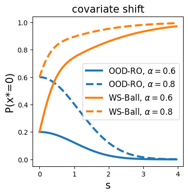
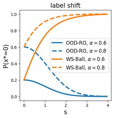
Figure 1: The curves show how (x=0)superscript𝑥0\mathbb{P}(x^{*}=0) changes with the distribution shift extent s𝑠s. The label “OOD-RO” represents our approach and “WS-Ball” represents the worst-case approach. α𝛼\alpha denotes the risk level. As s𝑠s increases, our “OOD-RO” becomes less conservative, with (x=0)superscript𝑥0\mathbb{P}(x^{*}=0) decreasing to 00, whereas the “WS-Ball” becomes increasingly conservative.

We can do the same calculation for the case of label shift, where the details are deferred to Appendix B. Figure 1 summarizes the two cases to compare our approach (which accounts for the shift structure) against the worst-case ball approach under two target quantile levels α=0.6𝛼0.6\alpha=0.6 and 0.80.80.8. For both cases, as s𝑠s increases, the mean of the covariate z𝑧z and the objective c𝑐c becomes more and more positive. If we utilize this structure and also the information from the covariate, we should be able to take a more aggressive decision by setting x=1x*=-1; this corresponds to the small probability of (x=0)superscript𝑥0\mathbb{P}(x^{*}=0) for our approach. However, if we do not take advantage of this shift structure, the worst-case ball has to be very large to cover the test distribution, and then a worst-case solution will result in a more and more conservative solution even as s𝑠s increases. This corresponds to the case in Corollary 1 if one adopts the naive density ratio w^1^𝑤1\hat{w}\equiv 1, the right-hand-side will have a term of DTV(𝒬,𝒫).subscript𝐷TV𝒬𝒫D_{\text{TV}}(\mathcal{Q},\mathcal{P}).

5 Experiments

In this section, we illustrate the performance of our proposed algorithm via one simple example. More experiments are deferred to Appendix C. Continue with problem (10), but instead of considering a single-dimensional z𝑧z, set a multi-dimensional covariate z=(z1,,zd)𝑧subscript𝑧1subscript𝑧𝑑z=(z_{1},\ldots,z_{d}). Let

c=(sign(z1)+ϵ)|z1|.𝑐signsubscript𝑧1italic-ϵsubscript𝑧1c=(\text{sign}(z_{1})+\epsilon)\cdot\sqrt{|z_{1}|}.

z𝑧z and ϵitalic-ϵ\epsilon are independent. The training distribution of z𝑧z and ϵitalic-ϵ\epsilon are 𝒩(𝟎,𝐈d)𝒩0subscript𝐈𝑑\mathcal{N}(\mathbf{0},\mathbf{I}_{d}) and 𝒩(0,0.1)𝒩00.1\mathcal{N}(0,0.1) respectively (let 𝟎0\mathbf{0} denote a zero vector of dimension d𝑑d, and 𝐈dsubscript𝐈𝑑\mathbf{I}_{d} an identity matrix of dimension d𝑑d). Covariate shift occurs in the test phase, where the mean of z𝑧z is shifted from 𝟎0\mathbf{0} to 𝟏dsubscript1𝑑\mathbf{1}_{d} (let 𝟏dsubscript1𝑑\mathbf{1}_{d} denote a d𝑑d-dimensional vector with all components equaling 111),

𝒫z=𝒩(𝟎,𝐈d)𝒬z=𝒩(𝟏d,𝐈d).subscript𝒫𝑧𝒩0subscript𝐈𝑑subscript𝒬𝑧𝒩subscript1𝑑subscript𝐈𝑑\mathcal{P}_{z}=\mathcal{N}(\mathbf{0},\mathbf{I}_{d})\longrightarrow\mathcal{Q}_{z}=\mathcal{N}(\mathbf{1}_{d},\mathbf{I}_{d}).

We study the performance of Algorithm 1 under different implementations of f^^𝑓\hat{f}, h^^\hat{h}, and w^^𝑤\hat{w}, as listed below. All neural networks used in this experiment are feed-forward networks with one hidden layer of 161616 neurons. We consider the following setups. Prediction models f^^𝑓\hat{f}: Lasso, random forest (“RF”), and neural network (“NN”). Quantile prediction models h^^\hat{h}: linear quantile regression (“Linear”), gradient boosting regression (“GBR”), and neural network. Density ratio estimators w^^𝑤\hat{w}: the trivial estimator (“Trivial”, w^1^𝑤1\hat{w}\equiv 1), the kernel mean matching method (“KMM”, (Gretton et al., 2008)), and the probabilistic classification method (“Cls-NN”, (Bickel et al., 2009)).

The risk level α=0.8𝛼0.8\alpha=0.8. The training dataset contains 400040004000 randomly generated samples, with 200020002000 of them used for learning f^^𝑓\hat{f}, 100010001000 for learning h^^\hat{h}, and 100010001000 for confidence adjustment. The test data contains 500050005000 samples from the shifted test distribution, with 400040004000 of them used to learn the density ratio estimator, and 100010001000 of them for evaluating the algorithm’s final performance. Unless otherwise stated, the default covariate dimension is d=4𝑑4d=4. We present the main results of our experiment below, with further details and additional experimental results provided in Appendix C.

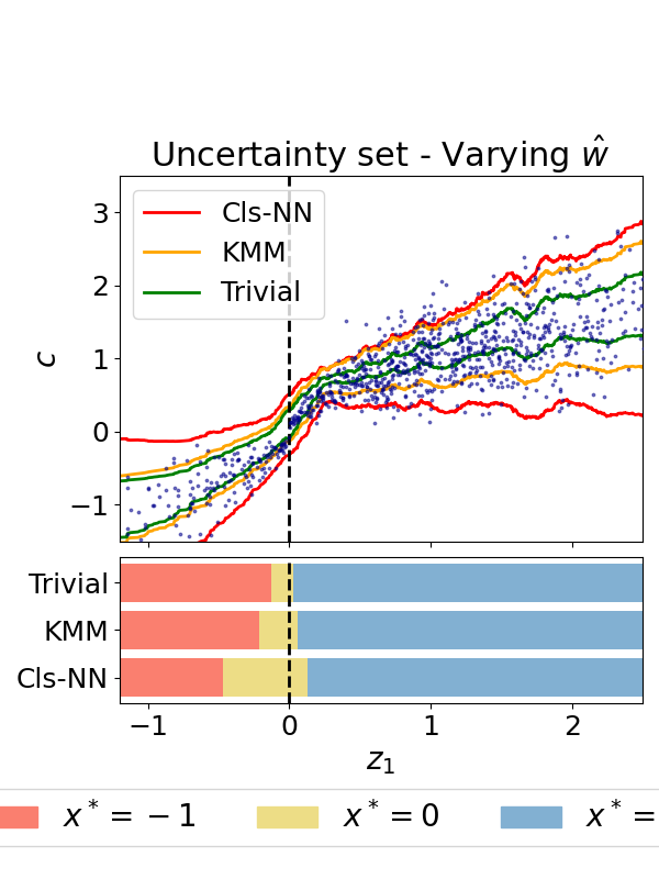
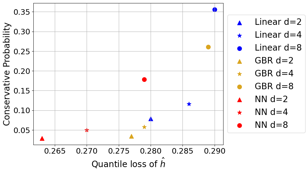
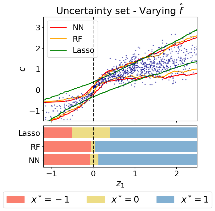
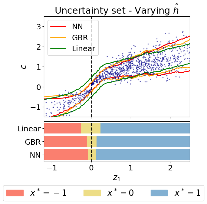
Prediction Models Boost Performance: In Figure 2, Algorithm 1 is evaluated under different implementations of f^^𝑓\hat{f} and h^^\hat{h}. The default configuration uses neural networks for f^^𝑓\hat{f} and h^^\hat{h}, and probabilistic classification for w^^𝑤\hat{w}. Except for the function component explicitly studied in the experiment, all other components follow the default configuration. Compared to the rest of the benchmarks, the neural network usually gives a better prediction, and Figure 2 demonstrates that this reduces the probability of getting a conservative solution x=0superscript𝑥0x^{*}=0. In Appendix C, we further show that neural networks give more precise predictions and that the probability of being conservative is positively correlated with the mean squared error of the prediction models.
Refer to caption
Refer to caption
Figure 2: Performance of Algorithm 1 under different prediction models f^^𝑓\hat{f} and quantile regression models h^^\hat{h}. Each scattered point indicates a random test sample. The colored curves and the region between them indicate the (conditional) uncertainty sets. The left panel implements different f^^𝑓\hat{f} with h^^\hat{h} fixed to be a neural network, and the right panel implements different h^^\hat{h}. The bar chart on the bottom indicates the corresponding optimal solution xsuperscript𝑥x^{*} for z1subscript𝑧1z_{1}’s from different regions. Implementing a better prediction model (the “NN”) generally reduces the probability of obtaining a conservative solution x=0superscript𝑥0x^{*}=0.

Density Ratio Estimator Avoids Mis-coverage: Now we illustrate the role of the density ratio estimator w^^𝑤\hat{w}. The left panel of Figure 3 demonstrates the algorithm’s performance under different w^^𝑤\hat{w}. The figure indicates that, if no reweighting is applied (i.e. “Trivially” estimate the density ratio to be 111), the empirical coverage rate can significantly drop below 0.80.80.8. A potentially misleading observation from the bar chart is that a “Trivial” estimator appears to be less conservative than its counterparts. However, as discussed above, this deceptive advantage is achieved at the cost of violating the coverage guarantee. The table on the right panel of Figure 3 reinforces the importance of a reliable density ratio estimator. By observing the “Total” rows of KMM and Cls-NN under different settings of the covariate dimension, we point out that a reliable density ratio estimator maintains the empirical coverage rate to be close to 0.80.80.8, even when the prediction models are poor. Another observation is that the coverage guarantee is approximately achieved in a conditional sense: after splitting the domain of z1subscript𝑧1z_{1} into two groups, with “z10subscript𝑧10z_{1}\leq 0” being a minority group and “z1>0subscript𝑧10z_{1}>0” being major, the empirical coverage rate remains approximately 0.80.80.8 for both groups.

Refer to caption
Trivial KMM Cls-NN
d=2𝑑2d=2 z10subscript𝑧10z_{1}\leq 0 0.80 0.77 0.79
z1>0subscript𝑧10z_{1}>0 0.78 0.75 0.77
Total 0.78 0.75 0.78
d=4𝑑4d=4 z10subscript𝑧10z_{1}\leq 0 0.56 0.72 0.79
z1>0subscript𝑧10z_{1}>0 0.54 0.86 0.81
Total 0.55 0.84 0.81
d=8𝑑8d=8 z10subscript𝑧10z_{1}\leq 0 0.53 0.71 0.86
z1>0subscript𝑧10z_{1}>0 0.4 0.76 0.81
Total 0.42 0.75 0.83
Figure 3: The figure on the left evaluates the performance of Algorithm 1 under different density ratio estimators w^^𝑤\hat{w}. With a better density ratio estimator (the “NN”), the coverage rate of the uncertainty sets is closer to the target level of 0.80.80.8. The table on the right gives the coverage rate of the uncertainty sets under different w^^𝑤\hat{w}, different covariate dimensions d𝑑d, and for different regions of z1subscript𝑧1z_{1}. For example, the row “z10subscript𝑧10z_{1}\leq 0” gives the coverage rate on samples with negative z1subscript𝑧1z_{1}, and the same holds for “z1>0subscript𝑧10z_{1}>0”. The “Total” rows give the coverage rate on the whole test dataset.

Discussions. In this paper, we study an out-of-distribution setting of robust optimization where the training distribution 𝒫𝒫\mathcal{P} might be different from the test distribution 𝒬.𝒬\mathcal{Q}. Other than the method, the analysis, and the numerical experiments, we hope such a study calls for more attention to the meaning of robustness in the context of robust optimization. As noted earlier, existing works consider mainly (i) robustness against the statistical gap between the empirical distribution supported on 𝒟Trsubscript𝒟Tr\mathcal{D}_{\text{Tr}} and the true distribution 𝒫𝒫\mathcal{P} or (ii) the robustness of a risk-sensitive objective such as VaR. Comparatively, the setting we study can be viewed as a robustness against distribution shift. Along this path, one may also consider the adversarial robustness where there might be a proportion of samples in the training data contaminated or adversarially generated from the other distributions than 𝒫𝒫\mathcal{P}. We believe the study of such more general notions of robustness deserves more future works.

References

  • Baker [1973] Charles R. Baker. Joint measures and cross-covariance operators. Transactions of the American Mathematical Society, 186:273–289, 1973. ISSN 00029947.
  • Ben-Tal et al. [2009] Aharon Ben-Tal, Laurent El Ghaoui, and Arkadi Nemirovski. Robust optimization, volume 28. Princeton university press, 2009.
  • Bertsimas and Kallus [2020] Dimitris Bertsimas and Nathan Kallus. From predictive to prescriptive analytics. Management Science, 66(3):1025–1044, 2020.
  • Bertsimas and Van Parys [2022] Dimitris Bertsimas and Bart Van Parys. Bootstrap robust prescriptive analytics. Mathematical Programming, 195(1-2):39–78, 2022.
  • Bickel et al. [2009] Steffen Bickel, Michael Brückner, and Tobias Scheffer. Discriminative learning under covariate shift. Journal of Machine Learning Research, 10(9), 2009.
  • Cao [2024] Guyang Kevin Cao. Non-Parameteric Conformal Distributionally Robust Optimization. PhD thesis, University of Michigan, 2024.
  • Chen and Kılınç-Karzan [2020] Violet Xinying Chen and Fatma Kılınç-Karzan. Online convex optimization perspective for learning from dynamically revealed preferences. arXiv preprint arXiv:2008.10460, 2020.
  • Chen et al. [2007] Xin Chen, Melvyn Sim, and Peng Sun. A robust optimization perspective on stochastic programming. Operations Research, 55(6):1058–1071, 2007.
  • Chenreddy et al. [2022] Abhilash Reddy Chenreddy, Nymisha Bandi, and Erick Delage. Data-driven conditional robust optimization. Advances in Neural Information Processing Systems, 35:9525–9537, 2022.
  • Duchi et al. [2023] John Duchi, Tatsunori Hashimoto, and Hongseok Namkoong. Distributionally robust losses for latent covariate mixtures. Operations Research, 71(2):649–664, 2023.
  • Elmachtoub and Grigas [2022] Adam N Elmachtoub and Paul Grigas. Smart "predict, then optimize". Management Science, 68(1):9–26, 2022.
  • Esteban-Pérez and Morales [2022] Adrián Esteban-Pérez and Juan M Morales. Distributionally robust stochastic programs with side information based on trimmings. Mathematical Programming, 195(1-2):1069–1105, 2022.
  • Fukumizu et al. [2004] Kenji Fukumizu, Francis R Bach, and Michael I Jordan. Dimensionality reduction for supervised learning with reproducing kernel hilbert spaces. Journal of Machine Learning Research, 5(Jan):73–99, 2004.
  • Ghaoui et al. [2003] Laurent El Ghaoui, Maksim Oks, and Francois Oustry. Worst-case value-at-risk and robust portfolio optimization: A conic programming approach. Operations Research, 51(4):543–556, 2003.
  • Goerigk and Kurtz [2020] Marc Goerigk and Jannis Kurtz. Data-driven robust optimization using unsupervised deep learning. arXiv preprint arXiv:2011.09769, 2020.
  • Gretton et al. [2008] Arthur Gretton, Alex Smola, Jiayuan Huang, Marcel Schmittfull, Karsten Borgwardt, and Bernhard Schölkopf. Covariate shift by kernel mean matching. 2008.
  • Ho-Nguyen and Kılınç-Karzan [2022] Nam Ho-Nguyen and Fatma Kılınç-Karzan. Risk guarantees for end-to-end prediction and optimization processes. Management Science, 68(12):8680–8698, 2022.
  • Hu et al. [2022] Yichun Hu, Nathan Kallus, and Xiaojie Mao. Fast rates for contextual linear optimization. Management Science, 68(6):4236–4245, 2022.
  • Huang et al. [2006] Jiayuan Huang, Arthur Gretton, Karsten Borgwardt, Bernhard Schölkopf, and Alex Smola. Correcting sample selection bias by unlabeled data. Advances in neural information processing systems, 19, 2006.
  • Huang and Gupta [2024] Michael Huang and Vishal Gupta. Learning best-in-class policies for the predict-then-optimize framework. arXiv preprint arXiv:2402.03256, 2024.
  • Jin and Candès [2023] Ying Jin and Emmanuel J Candès. Model-free selective inference under covariate shift via weighted conformal p-values. arXiv preprint arXiv:2307.09291, 2023.
  • Kannan et al. [2020] Rohit Kannan, Güzin Bayraksan, and James R Luedtke. Residuals-based distributionally robust optimization with covariate information. arXiv preprint arXiv:2012.01088, 2020.
  • Kannan et al. [2022] Rohit Kannan, Güzin Bayraksan, and James R Luedtke. Data-driven sample average approximation with covariate information. arXiv preprint arXiv:2207.13554, 2022.
  • Kpotufe [2017] Samory Kpotufe. Lipschitz density-ratios, structured data, and data-driven tuning. In Artificial Intelligence and Statistics, pages 1320–1328. PMLR, 2017.
  • Lin et al. [2024] Bo Lin, Erick Delage, and Timothy CY Chan. Conformal inverse optimization. arXiv preprint arXiv:2402.01489, 2024.
  • Lipton et al. [2018] Zachary Lipton, Yu-Xiang Wang, and Alexander Smola. Detecting and correcting for label shift with black box predictors. In International conference on machine learning, pages 3122–3130. PMLR, 2018.
  • Ma et al. [2023] Cong Ma, Reese Pathak, and Martin J Wainwright. Optimally tackling covariate shift in rkhs-based nonparametric regression. The Annals of Statistics, 51(2):738–761, 2023.
  • Natarajan et al. [2008] Karthik Natarajan, Dessislava Pachamanova, and Melvyn Sim. Incorporating asymmetric distributional information in robust value-at-risk optimization. Management Science, 54(3):573–585, 2008.
  • Ohmori [2021] Shunichi Ohmori. A predictive prescription using minimum volume k-nearest neighbor enclosing ellipsoid and robust optimization. Mathematics, 9(2):119, 2021.
  • Patel et al. [2024] Yash P Patel, Sahana Rayan, and Ambuj Tewari. Conformal contextual robust optimization. In International Conference on Artificial Intelligence and Statistics, pages 2485–2493. PMLR, 2024.
  • Podkopaev and Ramdas [2021] Aleksandr Podkopaev and Aaditya Ramdas. Distribution-free uncertainty quantification for classification under label shift. In Uncertainty in artificial intelligence, pages 844–853. PMLR, 2021.
  • Sadana et al. [2024] Utsav Sadana, Abhilash Chenreddy, Erick Delage, Alexandre Forel, Emma Frejinger, and Thibaut Vidal. A survey of contextual optimization methods for decision-making under uncertainty. European Journal of Operational Research, 2024.
  • Shimodaira [2000] Hidetoshi Shimodaira. Improving predictive inference under covariate shift by weighting the log-likelihood function. Journal of statistical planning and inference, 90(2):227–244, 2000.
  • Song et al. [2009] Le Song, Jonathan Huang, Alex Smola, and Kenji Fukumizu. Hilbert space embeddings of conditional distributions with applications to dynamical systems. In Proceedings of the 26th Annual International Conference on Machine Learning, pages 961–968, 2009.
  • Steinwart [2002] Ingo Steinwart. Support vector machines are universally consistent. Journal of Complexity, 18(3):768–791, 2002.
  • Sun et al. [2023a] Chunlin Sun, Linyu Liu, and Xiaocheng Li. Predict-then-calibrate: A new perspective of robust contextual lp. Advances in Neural Information Processing Systems, 36:17713–17741, 2023a.
  • Sun et al. [2023b] Chunlin Sun, Shang Liu, and Xiaocheng Li. Maximum optimality margin: A unified approach for contextual linear programming and inverse linear programming. In International Conference on Machine Learning, pages 32886–32912. PMLR, 2023b.
  • Tibshirani et al. [2019] Ryan J Tibshirani, Rina Foygel Barber, Emmanuel Candes, and Aaditya Ramdas. Conformal prediction under covariate shift. Advances in neural information processing systems, 32, 2019.
  • Wang et al. [2024] Tianyu Wang, Ningyuan Chen, and Chun Wang. Contextual optimization under covariate shift: A robust approach by intersecting wasserstein balls. arXiv preprint arXiv:2406.02426, 2024.
  • Wilder et al. [2019] Bryan Wilder, Bistra Dilkina, and Milind Tambe. Melding the data-decisions pipeline: Decision-focused learning for combinatorial optimization. In Proceedings of the AAAI Conference on Artificial Intelligence, volume 33, pages 1658–1665, 2019.
  • Zhang et al. [2013] Kun Zhang, Bernhard Schölkopf, Krikamol Muandet, and Zhikun Wang. Domain adaptation under target and conditional shift. In International Conference on Machine Learning, pages 819–827. PMLR, 2013.

Appendix A Reproductive Kernel Hilbert Space and Kernel Mean Matching

A.1 RKHS

Let the tuple (,κ,𝒵)𝜅𝒵(\mathcal{F},\kappa,\mathcal{Z}) denote a reproductive kernel Hilbert space (RKHS) \mathcal{F} on the sample space 𝒵𝒵\mathcal{Z} with kernel κ𝜅\kappa. The RKHS is a Hilbert space of functions f:𝒵:𝑓𝒵f:\mathcal{Z}\to\mathbb{R}, on which the inner product ,subscript\langle\cdot,\cdot\rangle_{\mathcal{F}} satisfies the reproducing property:

f,κ(z,)=f(z),f,z𝒵.formulae-sequencesubscript𝑓𝜅𝑧𝑓𝑧formulae-sequencefor-all𝑓𝑧𝒵\langle f,\kappa(z,\cdot)\rangle_{\mathcal{F}}=f(z),\quad\forall f\in\mathcal{F},z\in\mathcal{Z}.

That said, the evaluation of function f𝑓f on a single point z𝑧z can be viewed as an inner product between function f𝑓f and the evaluation operator κ(z,)𝜅𝑧\kappa(z,\cdot). We define the feature map ϕ:𝒵:italic-ϕ𝒵\phi:\mathcal{Z}\to\mathcal{F} by ϕ[z]κ(z,)italic-ϕdelimited-[]𝑧𝜅𝑧\phi[z]\coloneqq\kappa(z,\cdot). Throughout this part, we will use the square bracket []delimited-[][\cdot] to denote mappings to functional spaces. Based on the reproducing property, the feature map satisfies ϕ[z],ϕ[z]=κ(z,z)subscriptitalic-ϕdelimited-[]𝑧italic-ϕdelimited-[]superscript𝑧𝜅𝑧superscript𝑧\langle\phi[z],\phi[z^{\prime}]\rangle_{\mathcal{F}}=\kappa(z,z^{\prime}) for all z,z𝒵𝑧superscript𝑧𝒵z,z^{\prime}\in\mathcal{Z}.

The kernel mean embedding of a probability distribution 𝒫zsubscript𝒫𝑧\mathcal{P}_{z} [Zhang et al., 2013], denoted by μ[]subscript𝜇delimited-[]\mu_{\mathcal{F}}[\cdot], is a mapping from the space of all the probability distributions on 𝒵𝒵\mathcal{Z} to \mathcal{F}. The mapping is given by

μ[𝒫z]𝔼Z𝒫z[ϕ[Z]].subscript𝜇delimited-[]subscript𝒫𝑧subscript𝔼similar-to𝑍subscript𝒫𝑧delimited-[]italic-ϕdelimited-[]𝑍\mu_{\mathcal{F}}[\mathcal{P}_{z}]\coloneqq\mathbb{E}_{Z\sim\mathcal{P}_{z}}[\phi[Z]].

The kernel κ𝜅\kappa is called characteristic if the kernel mean embedding is injective: for 𝒫z𝒫zsubscript𝒫𝑧superscriptsubscript𝒫𝑧\mathcal{P}_{z}\neq\mathcal{P}_{z}^{\prime}, it holds that μ[𝒫z]μ[𝒫z]subscript𝜇delimited-[]subscript𝒫𝑧subscript𝜇delimited-[]superscriptsubscript𝒫𝑧\mu_{\mathcal{F}}[\mathcal{P}_{z}]\neq\mu_{\mathcal{F}}[\mathcal{P}_{z}^{\prime}]. And following Huang et al. [2006], the operator μ[]subscript𝜇delimited-[]\mu_{\mathcal{F}}[\cdot] is bijective if κ𝜅\kappa is a universal kernel in the sense of Steinwart [2002]. The core idea of the kernel mean matching is estimate 𝒫zsubscript𝒫𝑧\mathcal{P}_{z} with a 𝒫^zsubscript^𝒫𝑧\hat{\mathcal{P}}_{z} satisfying μ[𝒫z]μ[𝒫^z]subscript𝜇delimited-[]subscript𝒫𝑧subscript𝜇delimited-[]subscript^𝒫𝑧\mu_{\mathcal{F}}[\mathcal{P}_{z}]\approx\mu_{\mathcal{F}}[\hat{\mathcal{P}}_{z}].

A.2 Cross-covariance Operator

Consider the joint random variable (Z,C)𝒵×𝒞𝑍𝐶𝒵𝒞(Z,C)\in\mathcal{Z}\times\mathcal{C}. Define two RKHS’s by (,κ,𝒵)𝜅𝒵(\mathcal{F},\kappa,\mathcal{Z}) and (𝒢,η,𝒞)𝒢𝜂𝒞(\mathcal{G},\eta,\mathcal{C}) respectively. Let 𝒫𝒫\mathcal{P} denote the joint distribution of (Z,C)𝑍𝐶(Z,C) and 𝒫z,𝒫csubscript𝒫𝑧subscript𝒫𝑐\mathcal{P}_{z},\mathcal{P}_{c} their marginal distributions respectively, then the cross-covariance operator 𝒜Z,Csubscript𝒜𝑍𝐶\mathcal{A}_{Z,C} (with the dependency on 𝒫𝒫\mathcal{P} omitted) is defined as [Baker, 1973]

𝒜Z,C𝔼(Z,C)𝒫[ϕ[Z]ψ[C]]𝔼Z𝒫z[ϕ[Z]]𝔼C𝒫c[ψ[C]].subscript𝒜𝑍𝐶subscript𝔼similar-to𝑍𝐶𝒫delimited-[]tensor-productitalic-ϕdelimited-[]𝑍𝜓delimited-[]𝐶tensor-productsubscript𝔼similar-to𝑍subscript𝒫𝑧delimited-[]italic-ϕdelimited-[]𝑍subscript𝔼similar-to𝐶subscript𝒫𝑐delimited-[]𝜓delimited-[]𝐶\mathcal{A}_{Z,C}\coloneqq\mathbb{E}_{(Z,C)\sim\mathcal{P}}\left[\phi[Z]\otimes\psi[C]\right]-\mathbb{E}_{Z\sim\mathcal{P}_{z}}[\phi[Z]]\otimes\mathbb{E}_{C\sim\mathcal{P}_{c}}[\psi[C]].

In the following, we will omit the explicit distribution of the random variable in the subscript of 𝔼𝔼\mathbb{E} and replace expressions like 𝔼(Z,C)𝒫subscript𝔼similar-to𝑍𝐶𝒫\mathbb{E}_{(Z,C)\sim\mathcal{P}} with 𝔼Z,Csubscript𝔼𝑍𝐶\mathbb{E}_{Z,C}. The operator 𝒜Z,C[]subscript𝒜𝑍𝐶delimited-[]\mathcal{A}_{Z,C}[\cdot] can be viewed as a mapping from 𝒢𝒢\mathcal{G} to \mathcal{F} in the following way: by noting that ψ[C],g𝒢=g(C)subscript𝜓delimited-[]𝐶𝑔𝒢𝑔𝐶\langle\psi[C],g\rangle_{\mathcal{G}}=g(C) for any g𝒢𝑔𝒢g\in\mathcal{G}, we can define 𝒜Z,C[g]subscript𝒜𝑍𝐶delimited-[]𝑔\mathcal{A}_{Z,C}[g] as

𝒜Z,C[g]𝔼Z,C[g(C)ϕ[Z]]𝔼C[g(C)]𝔼Z[ϕ[Z]].subscript𝒜𝑍𝐶delimited-[]𝑔subscript𝔼𝑍𝐶delimited-[]𝑔𝐶italic-ϕdelimited-[]𝑍subscript𝔼𝐶delimited-[]𝑔𝐶subscript𝔼𝑍delimited-[]italic-ϕdelimited-[]𝑍\mathcal{A}_{Z,C}[g]\coloneqq\mathbb{E}_{Z,C}[g(C)\cdot\phi[Z]]-\mathbb{E}_{C}[g(C)]\cdot\mathbb{E}_{Z}[\phi[Z]].

For any functions f𝑓f\in\mathcal{F} and g𝒢𝑔𝒢g\in\mathcal{G}, the cross-covariace operator has the following property:

f,𝒜Z,C[g]=𝔼Z,C[f(Z)g(C)]𝔼Z[f(Z)]𝔼C[g(C)],subscript𝑓subscript𝒜𝑍𝐶delimited-[]𝑔subscript𝔼𝑍𝐶delimited-[]𝑓𝑍𝑔𝐶subscript𝔼𝑍delimited-[]𝑓𝑍subscript𝔼𝐶delimited-[]𝑔𝐶\langle f,\mathcal{A}_{Z,C}[g]\rangle_{\mathcal{F}}=\mathbb{E}_{Z,C}[f(Z)\cdot g(C)]-\mathbb{E}_{Z}[f(Z)]\cdot\mathbb{E}_{C}[g(C)],

which exactly corresponds to the covariance between f(Z)𝑓𝑍f(Z) and g(C)𝑔𝐶g(C). The conditional embedding operator 𝒰Z|Csubscript𝒰conditional𝑍𝐶\mathcal{U}_{Z|C} is a mapping from 𝒢𝒢\mathcal{G} to \mathcal{F} such that, for any c𝒞𝑐𝒞c\in\mathcal{C}, the follow equation holds:

𝒰Z|C[ψ(c)]=μ[𝒫z|c].subscript𝒰conditional𝑍𝐶delimited-[]𝜓𝑐subscript𝜇delimited-[]subscript𝒫conditional𝑧𝑐\mathcal{U}_{Z|C}[\psi(c)]=\mu_{\mathcal{F}}[\mathcal{P}_{z|c}]. (15)

In other words, 𝒰Z|Csubscript𝒰conditional𝑍𝐶\mathcal{U}_{Z|C} maps the feature map ψ(c)𝜓𝑐\psi(c) to the kernel mean embedding of the conditional distribution Z|C=cconditional𝑍𝐶𝑐Z|C=c. Following Song et al. [2009], if the cross-covariance operator 𝒜C,Csubscript𝒜𝐶𝐶\mathcal{A}_{C,C} is invertible, by defining

𝒰Z|C𝒜Z,C𝒜C,C1subscript𝒰conditional𝑍𝐶subscript𝒜𝑍𝐶superscriptsubscript𝒜𝐶𝐶1\mathcal{U}_{Z|C}\coloneqq\mathcal{A}_{Z,C}\mathcal{A}_{C,C}^{-1}

the equation (15) is satisfied. To see this, it is sufficient to show that f,𝒜Z,C𝒜C,C1[ψ[c]]=f,μ[𝒫z|c]subscript𝑓subscript𝒜𝑍𝐶superscriptsubscript𝒜𝐶𝐶1delimited-[]𝜓delimited-[]𝑐subscript𝑓subscript𝜇delimited-[]subscript𝒫conditional𝑧𝑐\langle f,\mathcal{A}_{Z,C}\mathcal{A}_{C,C}^{-1}[\psi[c]]\rangle_{\mathcal{F}}=\langle f,\mu_{\mathcal{F}}[\mathcal{P}_{z|c}]\rangle_{\mathcal{F}} for all f𝑓f\in\mathcal{F}, and this holds following the derivations below,

f,μ[𝒫z|c]subscript𝑓subscript𝜇delimited-[]subscript𝒫conditional𝑧𝑐\displaystyle\langle f,\mu_{\mathcal{F}}[\mathcal{P}_{z|c}]\rangle_{\mathcal{F}} =𝔼z|c[f(Z)|c]absentsubscript𝔼conditional𝑧𝑐delimited-[]conditional𝑓𝑍𝑐\displaystyle=\mathbb{E}_{z|c}[f(Z)|c]
=𝔼z|c[f(Z)|C],ψ[c]𝒢absentsubscriptsubscript𝔼conditional𝑧𝑐delimited-[]conditional𝑓𝑍𝐶𝜓delimited-[]𝑐𝒢\displaystyle=\langle\mathbb{E}_{z|c}[f(Z)|C],\psi[c]\rangle_{\mathcal{G}}
=𝒜C,C[𝔼z|c[f(Z)|C]],𝒜C,C1[ψ[c]]𝒢absentsubscriptsubscript𝒜𝐶𝐶delimited-[]subscript𝔼conditional𝑧𝑐delimited-[]conditional𝑓𝑍𝐶superscriptsubscript𝒜𝐶𝐶1delimited-[]𝜓delimited-[]𝑐𝒢\displaystyle=\langle\mathcal{A}_{C,C}[\mathbb{E}_{z|c}[f(Z)|C]],\mathcal{A}_{C,C}^{-1}[\psi[c]]\rangle_{\mathcal{G}}
=𝒜C,Z[f],𝒜C,C1[ψ[c]]𝒢absentsubscriptsubscript𝒜𝐶𝑍delimited-[]𝑓superscriptsubscript𝒜𝐶𝐶1delimited-[]𝜓delimited-[]𝑐𝒢\displaystyle=\langle\mathcal{A}_{C,Z}[f],\mathcal{A}_{C,C}^{-1}[\psi[c]]\rangle_{\mathcal{G}}
=f,𝒜Z,C𝒜C,C1[ψ[c]].absentsubscript𝑓subscript𝒜𝑍𝐶superscriptsubscript𝒜𝐶𝐶1delimited-[]𝜓delimited-[]𝑐\displaystyle=\langle f,\mathcal{A}_{Z,C}\mathcal{A}_{C,C}^{-1}[\psi[c]]\rangle_{\mathcal{F}}.

Equation (15) directly implies the following property, which serves as the key step of the KMM procedure in the density ratio estimation method of Zhang et al. [2013]:

𝒰Z|C[μ𝒢[𝒫c]]=μ[𝒫z].subscript𝒰conditional𝑍𝐶delimited-[]subscript𝜇𝒢delimited-[]subscript𝒫𝑐subscript𝜇delimited-[]subscript𝒫𝑧\mathcal{U}_{Z|C}[\mu_{\mathcal{G}}[\mathcal{P}_{c}]]=\mu_{\mathcal{F}}[\mathcal{P}_{z}].

A.3 Empirical Estimations

In this section, we briefly outline how to estimate the quantities above using i.i.d. samples (zi,ci)i=1Nsuperscriptsubscriptsubscript𝑧𝑖subscript𝑐𝑖𝑖1𝑁{(z_{i},c_{i})}_{i=1}^{N} drawn from 𝒫𝒫\mathcal{P}. By Mercer’s theorem, the feature map ϕ[z]italic-ϕdelimited-[]𝑧\phi[z] can be represented as a column vector in a (possibly infinite-dimensional) Hilbert space. We use ϕ[z]ψ[c]italic-ϕdelimited-[]𝑧𝜓superscriptdelimited-[]𝑐top\phi[z]\psi[c]^{\top} to denote the outer product ϕ[z]ψ[c]tensor-productitalic-ϕdelimited-[]𝑧𝜓delimited-[]𝑐\phi[z]\otimes\psi[c]. Define the matrices 𝚽(ϕ[z1],,ϕ[zN])𝚽italic-ϕdelimited-[]subscript𝑧1italic-ϕdelimited-[]subscript𝑧𝑁\mathbf{\Phi}\coloneqq(\phi[z_{1}],\dots,\phi[z_{N}]) and 𝚿(ψ[c1],,ψ[cN])𝚿𝜓delimited-[]subscript𝑐1𝜓delimited-[]subscript𝑐𝑁\mathbf{\Psi}\coloneqq(\psi[c_{1}],\dots,\psi[c_{N}]). Further define 𝐊,𝐇N×N𝐊𝐇superscript𝑁𝑁\mathbf{K},\mathbf{H}\in\mathbb{R}^{N\times N} with Ki,j=κ(zi,zj)subscript𝐾𝑖𝑗𝜅subscript𝑧𝑖subscript𝑧𝑗K_{i,j}=\kappa(z_{i},z_{j}) and Hi,j=η(ci,cj)subscript𝐻𝑖𝑗𝜂subscript𝑐𝑖subscript𝑐𝑗H_{i,j}=\eta(c_{i},c_{j}). The empirical estimators are indicated by adding a hat symbol ^^\hat{\cdot} to the original quantities, with their explicit expressions shown below:

μ[𝒫z]μ^subscript𝜇delimited-[]subscript𝒫𝑧subscript^𝜇\displaystyle\mu_{\mathcal{F}}[\mathcal{P}_{z}]\approx\hat{\mu}_{\mathcal{F}} 1Ni=1Nϕ(zi),absent1𝑁superscriptsubscript𝑖1𝑁italic-ϕsubscript𝑧𝑖\displaystyle\coloneqq\dfrac{1}{N}\sum_{i=1}^{N}\phi(z_{i}),
μ𝒢[𝒫c]μ^𝒢subscript𝜇𝒢delimited-[]subscript𝒫𝑐subscript^𝜇𝒢\displaystyle\mu_{\mathcal{G}}[\mathcal{P}_{c}]\approx\hat{\mu}_{\mathcal{G}} 1Ni=1Nψ(ci),absent1𝑁superscriptsubscript𝑖1𝑁𝜓subscript𝑐𝑖\displaystyle\coloneqq\dfrac{1}{N}\sum_{i=1}^{N}\psi(c_{i}),
𝒜Z,C𝒜^Z,Csubscript𝒜𝑍𝐶subscript^𝒜𝑍𝐶\displaystyle\mathcal{A}_{Z,C}\approx\hat{\mathcal{A}}_{Z,C} 1N(𝚽μ^𝟏)(𝚿μ^𝒢𝟏)absent1𝑁𝚽subscript^𝜇superscript1topsuperscript𝚿subscript^𝜇𝒢superscript1toptop\displaystyle\coloneqq\dfrac{1}{N}(\mathbf{\Phi}-\hat{\mu}_{\mathcal{F}}\mathbf{1}^{\top})(\mathbf{\Psi}-\hat{\mu}_{\mathcal{G}}\mathbf{1}^{\top})^{\top}
=1N𝚽(I1N𝟏𝟏)𝚿,absent1𝑁𝚽𝐼1𝑁superscript11topsuperscript𝚿top\displaystyle=\dfrac{1}{N}\mathbf{\Phi}\left(I-\frac{1}{N}\mathbf{1}\mathbf{1}^{\top}\right)\mathbf{\Psi}^{\top},
𝒜C,C1𝒜^C,C1superscriptsubscript𝒜𝐶𝐶1superscriptsubscript^𝒜𝐶𝐶1\displaystyle\mathcal{A}_{C,C}^{-1}\approx\hat{\mathcal{A}}_{C,C}^{-1} N𝚿𝐇1(I1N𝟏𝟏)1𝐇1𝚿,absent𝑁𝚿superscript𝐇1superscript𝐼1𝑁superscript11top1superscript𝐇1superscript𝚿top\displaystyle\coloneqq N\cdot\mathbf{\Psi}\mathbf{H}^{-1}\left(I-\frac{1}{N}\mathbf{1}\mathbf{1}^{\top}\right)^{-1}\mathbf{H}^{-1}\mathbf{\Psi}^{\top},
𝒰Z|C𝒰^Z|Csubscript𝒰conditional𝑍𝐶subscript^𝒰conditional𝑍𝐶\displaystyle\mathcal{U}_{Z|C}\approx\hat{\mathcal{U}}_{Z|C} 𝚽𝐇1𝚿.absent𝚽superscript𝐇1superscript𝚿top\displaystyle\coloneqq\mathbf{\Phi}\mathbf{H}^{-1}\mathbf{\Psi}^{\top}.

Appendix B Illustrative Example

Consider the illustrative example:

minxsubscript𝑥\displaystyle\min_{x}\ VaRα𝒬(cx|z)s.t.1x1,superscriptsubscriptVaR𝛼𝒬conditional𝑐𝑥𝑧s.t.1𝑥1\displaystyle\ \text{VaR}_{\alpha}^{\mathcal{Q}}(c\cdot x|z)\ \ \text{s.t.}\ -1\leq x\leq 1, (16)

where α(0.5,1)𝛼0.51\alpha\in(0.5,1) and c=z+ϵ𝑐𝑧italic-ϵc=z+\epsilon. In the training distribution 𝒫𝒫\mathcal{P}, the z𝑧z and ϵitalic-ϵ\epsilon are independent and respectively follow 𝒩(0,σ12)𝒩0superscriptsubscript𝜎12\mathcal{N}(0,\sigma_{1}^{2}) and 𝒩(0,σ22)𝒩0superscriptsubscript𝜎22\mathcal{N}(0,\sigma_{2}^{2}). We list the explicit expressions for the following probability distributions:

𝒫z=𝒩(0,σ12),𝒫c=𝒩(0,σ12+σ22),formulae-sequencesubscript𝒫𝑧𝒩0superscriptsubscript𝜎12subscript𝒫𝑐𝒩0superscriptsubscript𝜎12superscriptsubscript𝜎22\mathcal{P}_{z}=\mathcal{N}(0,\sigma_{1}^{2}),\quad\mathcal{P}_{c}=\mathcal{N}(0,\sigma_{1}^{2}+\sigma_{2}^{2}),
𝒫c|z=𝒩(z,σ22),𝒫z|c=𝒩(σ12cσ12+σ22,σ12σ22σ12+σ22),formulae-sequencesubscript𝒫conditional𝑐𝑧𝒩𝑧superscriptsubscript𝜎22subscript𝒫conditional𝑧𝑐𝒩superscriptsubscript𝜎12𝑐superscriptsubscript𝜎12superscriptsubscript𝜎22superscriptsubscript𝜎12superscriptsubscript𝜎22superscriptsubscript𝜎12superscriptsubscript𝜎22\mathcal{P}_{c|z}=\mathcal{N}(z,\sigma_{2}^{2}),\quad\mathcal{P}_{z|c}=\mathcal{N}\left(\frac{\sigma_{1}^{2}\cdot c}{\sigma_{1}^{2}+\sigma_{2}^{2}},\frac{\sigma_{1}^{2}\sigma_{2}^{2}}{\sigma_{1}^{2}+\sigma_{2}^{2}}\right),
(c,z)𝒫=𝒩((00),(σ12+σ22σ12σ12σ12)).similar-to𝑐𝑧𝒫𝒩matrix00matrixsuperscriptsubscript𝜎12superscriptsubscript𝜎22superscriptsubscript𝜎12superscriptsubscript𝜎12superscriptsubscript𝜎12(c,z)\sim\mathcal{P}=\mathcal{N}\left(\begin{pmatrix}0\\ 0\end{pmatrix},\begin{pmatrix}\sigma_{1}^{2}+\sigma_{2}^{2}&\sigma_{1}^{2}\\ \sigma_{1}^{2}&\sigma_{1}^{2}\end{pmatrix}\right).

We describe the explicit form of 𝒬𝒬\mathcal{Q} under the following two distribution shift scenarios:

  • Covariate shift: let s𝑠s represent the extent of covariate shift. The distribution of z𝑧z is shifted from 𝒫z=𝒩(0,σ12)subscript𝒫𝑧𝒩0superscriptsubscript𝜎12\mathcal{P}_{z}=\mathcal{N}(0,\sigma_{1}^{2}) to 𝒬z=𝒩(s,σ12)subscript𝒬𝑧𝒩𝑠superscriptsubscript𝜎12\mathcal{Q}_{z}=\mathcal{N}(s,\sigma_{1}^{2}), while the conditional distribution of c|zconditional𝑐𝑧c|z remains to be 𝒩(z,σ22)𝒩𝑧superscriptsubscript𝜎22\mathcal{N}(z,\sigma_{2}^{2}). The joint distribution of (c,z)𝑐𝑧(c,z) is shifted to 𝒬=𝒩((ss),(σ12+σ22σ12σ12σ12))𝒬𝒩matrix𝑠𝑠matrixsuperscriptsubscript𝜎12superscriptsubscript𝜎22superscriptsubscript𝜎12superscriptsubscript𝜎12superscriptsubscript𝜎12\mathcal{Q}=\mathcal{N}\left(\begin{pmatrix}s\\ s\end{pmatrix},\begin{pmatrix}\sigma_{1}^{2}+\sigma_{2}^{2}&\sigma_{1}^{2}\\ \sigma_{1}^{2}&\sigma_{1}^{2}\end{pmatrix}\right).

  • Label shift: let s𝑠s represent the extent of label shift. The distribution of c𝑐c is shifted from 𝒫c=𝒩(0,σ12+σ22)subscript𝒫𝑐𝒩0superscriptsubscript𝜎12superscriptsubscript𝜎22\mathcal{P}_{c}=\mathcal{N}(0,\sigma_{1}^{2}+\sigma_{2}^{2}) to 𝒬c=𝒩(s,σ12+σ22)subscript𝒬𝑐𝒩𝑠superscriptsubscript𝜎12superscriptsubscript𝜎22\mathcal{Q}_{c}=\mathcal{N}(s,\sigma_{1}^{2}+\sigma_{2}^{2}), while the conditional distribution z|cconditional𝑧𝑐z|c remains to be 𝒩(σ12cσ12+σ22,σ12σ22σ12+σ22)𝒩superscriptsubscript𝜎12𝑐superscriptsubscript𝜎12superscriptsubscript𝜎22superscriptsubscript𝜎12superscriptsubscript𝜎22superscriptsubscript𝜎12superscriptsubscript𝜎22\mathcal{N}\left(\frac{\sigma_{1}^{2}\cdot c}{\sigma_{1}^{2}+\sigma_{2}^{2}},\frac{\sigma_{1}^{2}\sigma_{2}^{2}}{\sigma_{1}^{2}+\sigma_{2}^{2}}\right). It follows that the distribution of z𝑧z in 𝒬𝒬\mathcal{Q} is shifted to 𝒩(σ12sσ12+σ22,σ12)𝒩superscriptsubscript𝜎12𝑠superscriptsubscript𝜎12superscriptsubscript𝜎22superscriptsubscript𝜎12\mathcal{N}\left(\frac{\sigma_{1}^{2}\cdot s}{\sigma_{1}^{2}+\sigma_{2}^{2}},\sigma_{1}^{2}\right), and the distribution of ϵitalic-ϵ\epsilon is shifted to 𝒩(σ22sσ12+σ22,σ22)𝒩superscriptsubscript𝜎22𝑠superscriptsubscript𝜎12superscriptsubscript𝜎22superscriptsubscript𝜎22\mathcal{N}\left(\frac{\sigma_{2}^{2}\cdot s}{\sigma_{1}^{2}+\sigma_{2}^{2}},\sigma_{2}^{2}\right). The joint distribution of (c,z)𝑐𝑧(c,z) is shifted to 𝒬=𝒩((sσ12sσ12+σ22),(σ12+σ22σ12σ12σ12))𝒬𝒩matrix𝑠superscriptsubscript𝜎12𝑠superscriptsubscript𝜎12superscriptsubscript𝜎22matrixsuperscriptsubscript𝜎12superscriptsubscript𝜎22superscriptsubscript𝜎12superscriptsubscript𝜎12superscriptsubscript𝜎12\mathcal{Q}=\mathcal{N}\left(\begin{pmatrix}s\\ \frac{\sigma_{1}^{2}\cdot s}{\sigma_{1}^{2}+\sigma_{2}^{2}}\end{pmatrix},\begin{pmatrix}\sigma_{1}^{2}+\sigma_{2}^{2}&\sigma_{1}^{2}\\ \sigma_{1}^{2}&\sigma_{1}^{2}\end{pmatrix}\right).

The solution to (16) admits a simple form under the idealized setting, as given in (11) and restated below:

x={1,VaRα𝒬(c|z)0,1,VaR1α𝒬(c|z)0,0,otherwise,x^{*}=\left\{\begin{aligned} &1,&\text{VaR}^{\mathcal{Q}}_{\alpha}(c|z)\leq 0,\\ &-1,&\text{VaR}^{\mathcal{Q}}_{1-\alpha}(c|z)\geq 0,\\ &0,&\text{otherwise},\end{aligned}\right. (17)

The probability of yielding an over-conservative solution is

(x=0)superscript𝑥0\displaystyle\mathbb{P}(x^{*}=0) =z𝒬z(VaR1α(c|z)0VaRα(c|z)).absentsubscriptsimilar-to𝑧subscript𝒬𝑧subscriptVaR1𝛼conditional𝑐𝑧0subscriptVaR𝛼conditional𝑐𝑧\displaystyle=\mathbb{P}_{z\sim\mathcal{Q}_{z}}(\text{VaR}_{1-\alpha}(c|z)\leq 0\leq\text{VaR}_{\alpha}(c|z)). (18)

Specifically, in the covariate shift setting, the probability equals

(x=0)=Φ(σ2σ1Φ1(α)sσ1)Φ(σ2σ1Φ1(α)sσ1),superscript𝑥0Φsubscript𝜎2subscript𝜎1superscriptΦ1𝛼𝑠subscript𝜎1Φsubscript𝜎2subscript𝜎1superscriptΦ1𝛼𝑠subscript𝜎1\mathbb{P}(x^{*}=0)=\Phi\left(\frac{\sigma_{2}}{\sigma_{1}}\Phi^{-1}(\alpha)-\frac{s}{\sigma_{1}}\right)-\Phi\left(-\frac{\sigma_{2}}{\sigma_{1}}\Phi^{-1}(\alpha)-\frac{s}{\sigma_{1}}\right),

and in the label shift setting, the probability also equals

(x=0)=Φ(σ2σ1Φ1(α)sσ1)Φ(σ2σ1Φ1(α)sσ1).superscript𝑥0Φsubscript𝜎2subscript𝜎1superscriptΦ1𝛼𝑠subscript𝜎1Φsubscript𝜎2subscript𝜎1superscriptΦ1𝛼𝑠subscript𝜎1\mathbb{P}(x^{*}=0)=\Phi\left(\frac{\sigma_{2}}{\sigma_{1}}\Phi^{-1}(\alpha)-\frac{s}{\sigma_{1}}\right)-\Phi\left(-\frac{\sigma_{2}}{\sigma_{1}}\Phi^{-1}(\alpha)-\frac{s}{\sigma_{1}}\right).

Worst-case Approach

Alternative to our density ratio-based approach is the worst-case approach. Construct the worst-case ball:

(R){𝒩(r,(σ12+σ22σ12σ12σ12)):rR}.𝑅conditional-set𝒩𝑟matrixsuperscriptsubscript𝜎12superscriptsubscript𝜎22superscriptsubscript𝜎12superscriptsubscript𝜎12superscriptsubscript𝜎12norm𝑟𝑅\mathcal{B}(R)\coloneqq\left\{\mathcal{N}\left(r,\begin{pmatrix}\sigma_{1}^{2}+\sigma_{2}^{2}&\sigma_{1}^{2}\\ \sigma_{1}^{2}&\sigma_{1}^{2}\end{pmatrix}\right)\ :\ \|r\|\leq R\right\}.

Following the discussions in the main context, the objective of the worst-case approach is given by (13) and restated below:

minxmax𝒬(R)VaRα𝒬(cx|z)s.t.1x1.subscript𝑥subscript𝒬𝑅subscriptsuperscriptVaR𝒬𝛼conditional𝑐𝑥𝑧s.t.1𝑥1\min_{x}\max_{\mathcal{Q}\in\mathcal{B}(R)}\ \ \text{VaR}^{\mathcal{Q}}_{\alpha}(c\cdot x|z)\ \ \text{s.t.}\ -1\leq x\leq 1.

The probability of yielding an over-conservative solution is

(x=0)=z𝒬z(VaR¯1α(c|z)0VaR¯α(c|z)).superscript𝑥0subscriptsimilar-to𝑧subscript𝒬𝑧subscript¯VaR1𝛼conditional𝑐𝑧0subscript¯VaR𝛼conditional𝑐𝑧\mathbb{P}(x^{*}=0)=\mathbb{P}_{z\sim\mathcal{Q}_{z}}(\underline{\text{VaR}}_{1-\alpha}(c|z)\leq 0\leq\overline{\text{VaR}}_{\alpha}(c|z)).

In the covariate shift setting, we have R=2s𝑅2𝑠R=\sqrt{2}s in order that (R)𝑅\mathcal{B}(R) covers 𝒬𝒬\mathcal{Q}. In the label shift setting, R=1+σ14(σ12+σ22)2s𝑅1superscriptsubscript𝜎14superscriptsuperscriptsubscript𝜎12superscriptsubscript𝜎222𝑠R=\sqrt{1+\frac{\sigma_{1}^{4}}{(\sigma_{1}^{2}+\sigma_{2}^{2})^{2}}}\cdot s. The explicit form of the conservative probability is

(x=0)superscript𝑥0\displaystyle\mathbb{P}(x^{*}=0) =Φ(σ2σ1Φ1(α)+2sσ1sσ1)absentΦsubscript𝜎2subscript𝜎1superscriptΦ1𝛼2𝑠subscript𝜎1𝑠subscript𝜎1\displaystyle=\Phi\left(\frac{\sigma_{2}}{\sigma_{1}}\Phi^{-1}(\alpha)+\frac{\sqrt{2}\cdot s}{\sigma_{1}}-\frac{s}{\sigma_{1}}\right)
Φ(σ2σ1Φ1(α)2sσ1sσ1)Φsubscript𝜎2subscript𝜎1superscriptΦ1𝛼2𝑠subscript𝜎1𝑠subscript𝜎1\displaystyle\phantom{=}-\Phi\left(-\frac{\sigma_{2}}{\sigma_{1}}\Phi^{-1}(\alpha)-\frac{\sqrt{2}\cdot s}{\sigma_{1}}-\frac{s}{\sigma_{1}}\right)

for the covariate shift setting and

(x=0)superscript𝑥0\displaystyle\mathbb{P}(x^{*}=0) =Φ(σ2σ1Φ1(α)+1σ12+σ12(σ12+σ22)2sσ1sσ12+σ22)absentΦsubscript𝜎2subscript𝜎1superscriptΦ1𝛼1superscriptsubscript𝜎12superscriptsubscript𝜎12superscriptsuperscriptsubscript𝜎12superscriptsubscript𝜎222𝑠subscript𝜎1𝑠superscriptsubscript𝜎12superscriptsubscript𝜎22\displaystyle=\Phi\left(\frac{\sigma_{2}}{\sigma_{1}}\Phi^{-1}(\alpha)+\sqrt{\frac{1}{\sigma_{1}^{2}}+\frac{\sigma_{1}^{2}}{(\sigma_{1}^{2}+\sigma_{2}^{2})^{2}}}\cdot s-\frac{\sigma_{1}\cdot s}{\sigma_{1}^{2}+\sigma_{2}^{2}}\right)
Φ(σ2σ1Φ1(α)1σ12+σ12(σ12+σ22)2sσ1sσ12+σ22)Φsubscript𝜎2subscript𝜎1superscriptΦ1𝛼1superscriptsubscript𝜎12superscriptsubscript𝜎12superscriptsuperscriptsubscript𝜎12superscriptsubscript𝜎222𝑠subscript𝜎1𝑠superscriptsubscript𝜎12superscriptsubscript𝜎22\displaystyle\phantom{=}-\Phi\left(-\frac{\sigma_{2}}{\sigma_{1}}\Phi^{-1}(\alpha)-\sqrt{\frac{1}{\sigma_{1}^{2}}+\frac{\sigma_{1}^{2}}{(\sigma_{1}^{2}+\sigma_{2}^{2})^{2}}}\cdot s-\frac{\sigma_{1}\cdot s}{\sigma_{1}^{2}+\sigma_{2}^{2}}\right)

for the label shift setting.

Figure 1 is plotted by setting σ1=σ2=1subscript𝜎1subscript𝜎21\sigma_{1}=\sigma_{2}=1.

Appendix C More Experiments and Experiment Details

We consider several implementations of the three components: f^^𝑓\hat{f}, h^^\hat{h} and w^^𝑤\hat{w} for our Algorithm 1. For the expectation predictor f^^𝑓\hat{f} which predicts 𝔼[c|z]𝔼delimited-[]conditional𝑐𝑧\mathbb{E}[c|z] with z𝑧z, we consider using Lasso regression, random forest, and neural network. On different training datasets, the regularization parameter λ𝜆\lambda of the Lasso regression is selected as the optimal parameter in range [0,4]04[0,4]; for the random forest searches the best number of trees in range [100,1000]1001000[100,1000] and the best depth in range [10,80]1080[10,80]; the neural network has a single middle layer with 161616 neurons, with the learning rate set to 0.010.010.01 and the training epochs set to 500500500. For the quantile predictor h^^\hat{h}, we implement linear quantile regression, gradient boosting regression, and neural network, all trained by minimizing the quantile loss. For the density estimator, we mainly consider estimators for the covariate shift setting, including the trivial estimator, the kernel mean matching method introduced in Gretton et al. [2008], and the probabilistic classification method introduced in Bickel et al. [2009]. The computational complexity of the kernel mean matching method scales at least quadratically with the data size, so we only sample 200200200 data from the training distribution and 200200200 data from the test distribution to run the algorithm.

The performance metrics we consider include the coverage rate and the α𝛼\alpha-quantile of the objective cxsuperscript𝑐top𝑥c^{\top}x. Specifically, we evaluate the marginal and conditional coverage rates of the uncertainty sets generated from different implementations of our algorithm, and how different they are from the target coverage rate. The α𝛼\alpha-quantile of the objective, denoted by VaRα𝒬(cx|z)superscriptsubscriptVaR𝛼𝒬conditionalsuperscript𝑐top𝑥𝑧\mathrm{VaR}_{\alpha}^{\mathcal{Q}}(c^{\top}x|z), is evaluated by generating 100100100 samples of c𝑐c from the underlying conditional distribution 𝒬c|zsubscript𝒬conditional𝑐𝑧\mathcal{Q}_{c|z} and then calculate the empirical α𝛼\alpha-quantile of cxsuperscript𝑐top𝑥c^{\top}x.

C.1 Additional Experiments on the Simple Example

This section presents additional experimental results for the simple optimization problem discussed in Section 5. In Figure 4, we experiment with different choices of f^^𝑓\hat{f} and h^^\hat{h}, and different covariate dimensions d𝑑d. Specifically, the implementations of f^^𝑓\hat{f} and h^^\hat{h} follow the setup of Figure 2, and the d𝑑d’s we consider include d=2,4,8𝑑248d=2,4,8. Both the mean squared error and the quantile loss are evaluated on the test dataset, with the c𝑐c values known. The results indicate that the algorithm tends to perform better, as reflected by a lower conservative probability, when the prediction models f^^𝑓\hat{f} and h^^\hat{h} have lower prediction errors. Further, for both f^^𝑓\hat{f} and h^^\hat{h}, neural networks (NN) generally achieve strong predictive performance.
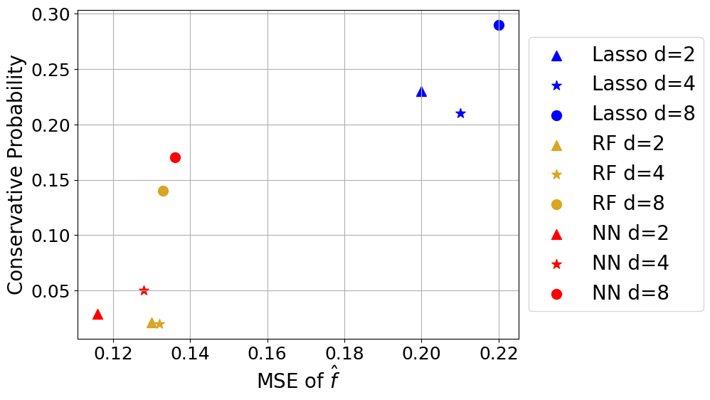
Refer to caption
Refer to caption
Figure 4: The quality of the predictors affects the performance of Algorithm 1. In the left figure, the x-axis represents the mean squared error (MSE) of f^^𝑓\hat{f} on the test dataset, while in the right figure, the x-axis represents the quantile loss of h^^\hat{h}. For both metrics, lower values indicate higher predictor quality. The y-axis shows the probability of obtaining an over-conservative solution at x=0superscript𝑥0x^{*}=0, where a lower probability indicates better algorithm performance. Both figures illustrate that improved prediction models enhance the performance of the algorithm.

C.2 Shortest Path Problem and Fractional Knapsack Problem

We test our algorithm on two practical LP settings. The risk level α𝛼\alpha is fixed to 0.80.80.8 and we consider the covariate shift of the test distribution.

The shortest path problem seeks a path between two vertices in a weighted graph such that the total accumulated cost along the path’s edges is minimized. Specifically, we consider the shortest path problem on a 5×5555\times 5 grid with 252525 nodes and 404040 edges. The objective is to find the shortest path from the top-left node to the bottom-right node. For i=0,,4𝑖04i=0,\ldots,4 and j=0,,4𝑗04j=0,\ldots,4, let (i,j)𝑖𝑗(i,j) denote the node on the i𝑖i-th row and j𝑗j-th column, with the top-left node located at the coordinate (0,0)00(0,0) and the bottom-right node at the coordinate (5,5)55(5,5). The tuple ((i,j),(i,j))esubscript𝑖𝑗superscript𝑖superscript𝑗𝑒((i,j),(i^{\prime},j^{\prime}))_{e} denotes the edge between node (i,j)𝑖𝑗(i,j) and (i,j)superscript𝑖superscript𝑗(i^{\prime},j^{\prime}). Let V𝑉V denote the set of all nodes and E𝐸E denote all edges. For ((i,j),(i,j))eEsubscript𝑖𝑗superscript𝑖superscript𝑗𝑒𝐸((i,j),(i^{\prime},j^{\prime}))_{e}\in E, use c(i,j),(i,j)subscript𝑐𝑖𝑗superscript𝑖superscript𝑗c_{(i,j),(i^{\prime},j^{\prime})} to represent the cost of the edge ((i,j),(i,j))esubscript𝑖𝑗superscript𝑖superscript𝑗𝑒((i,j),(i^{\prime},j^{\prime}))_{e} (for the undirected graph that we consider, set c(i,j),(i,j)=c(i,j),(i,j)subscript𝑐𝑖𝑗superscript𝑖superscript𝑗subscript𝑐superscript𝑖superscript𝑗𝑖𝑗c_{(i,j),(i^{\prime},j^{\prime})}=c_{(i^{\prime},j^{\prime}),(i,j)}). The decision variables are x(i,j),(i,j)subscript𝑥𝑖𝑗superscript𝑖superscript𝑗x_{(i,j),(i^{\prime},j^{\prime})} for all ((i,j),(i,j))eEsubscript𝑖𝑗superscript𝑖superscript𝑗𝑒𝐸((i,j),(i^{\prime},j^{\prime}))_{e}\in E, where x(i,j),(i,j)=1subscript𝑥𝑖𝑗superscript𝑖superscript𝑗1x_{(i,j),(i^{\prime},j^{\prime})}=1 denotes a directed path segment from the node (i,j)𝑖𝑗(i,j) to the node (i,j)superscript𝑖superscript𝑗(i^{\prime},j^{\prime}). The shortest path problem then has the following risk-sensitive LP formulation:

minxsubscript𝑥\displaystyle\min_{x} VaRα(((i,j),(i,j))eEc(i,j),(i,j)x(i,j),(i,j))subscriptVaR𝛼subscriptsubscript𝑖𝑗superscript𝑖superscript𝑗𝑒𝐸subscript𝑐𝑖𝑗superscript𝑖superscript𝑗subscript𝑥𝑖𝑗superscript𝑖superscript𝑗\displaystyle\ \text{VaR}_{\alpha}\left(\sum_{((i,j),(i^{\prime},j^{\prime}))_{e}\in E}c_{(i,j),(i^{\prime},j^{\prime})}\cdot x_{(i,j),(i^{\prime},j^{\prime})}\right) (19)
s.t. (i,j):((i,j),(i,j))eE(x(i,j),(i,j)x(i,j),(i,j))={1(i,j)=(0,0)1(i,j)=(4,4)0otherwise\displaystyle\ \sum_{(i^{\prime},j^{\prime}):((i,j),(i^{\prime},j^{\prime}))_{e}\in E}\left(x_{(i,j),(i^{\prime},j^{\prime})}-x_{(i^{\prime},j^{\prime}),(i,j)}\right)=\left\{\begin{aligned} 1&\quad(i,j)=(0,0)\\ -1&\quad(i,j)=(4,4)\\ 0&\quad\text{otherwise}\\ \end{aligned}\right.

Extending to the OOD robust formulation, we assume that the dynamic of the cost vector c40𝑐superscript40c\in\mathbb{R}^{40} is controlled by the covariate zd𝑧superscript𝑑z\in\mathbb{R}^{d} (we fix d=10𝑑10d=10 in this experiment) through

𝒫c|z((1dΘz+3)5+1)ϵ,similar-tosubscript𝒫conditional𝑐𝑧superscript1𝑑Θ𝑧351italic-ϵ\mathcal{P}_{c|z}\sim\left(\left(\frac{1}{\sqrt{d}}\Theta z+3\right)^{5}+1\right)\circ\epsilon,

where Θ40×dΘsuperscript40𝑑\Theta\in\mathbb{R}^{40\times d} is a 0-1 matrix with each entry generated independently from a Bernoulli(0.5)Bernoulli0.5\text{Bernoulli}(0.5) distribution. The ΘΘ\Theta matrix is fixed once it is generated. The \circ symbol denotes an elementwise multiplication. Each element of the random vector ϵ40italic-ϵsuperscript40\epsilon\in\mathbb{R}^{40} is generated independently from Uniform(34,54)Uniform3454\text{Uniform}(\frac{3}{4},\frac{5}{4}). In the training data, the covariate z𝑧z is generated from 𝒫z=𝒩(0,𝐈d)subscript𝒫𝑧𝒩0subscript𝐈𝑑\mathcal{P}_{z}=\mathcal{N}(0,\mathbf{I}_{d}), and in the test data z𝑧z is generated from 𝒬z=𝒩(𝟏d,𝐈d)subscript𝒬𝑧𝒩subscript1𝑑subscript𝐈𝑑\mathcal{Q}_{z}=\mathcal{N}(\mathbf{1}_{d},\mathbf{I}_{d}). The objective of the OOD formulation replaces the VaRα()subscriptVaR𝛼\text{VaR}_{\alpha}(\cdot) part in (19) with VaRα𝒬()superscriptsubscriptVaR𝛼𝒬\text{VaR}_{\alpha}^{\mathcal{Q}}(\cdot).

The fractional knapsack problem models the case where customers select items that maximize their utility, under a budget constraint. We consider a simple setting with 202020 items. The decision variables x=(x1,,x20)𝑥subscript𝑥1subscript𝑥20x=(x_{1},\ldots,x_{20}) denote the fractions (in range [0,1]01[0,1]) of items to purchase, c20𝑐superscript20c\in\mathbb{R}^{20} denote the item utilities, p20𝑝superscript20p\in\mathbb{R}^{20} denote the price of items, and B>0𝐵0B>0 the total budget. The fractional knapsack problem has the following risk-sensitive LP formulation:

minxsubscript𝑥\displaystyle\min_{x} VaRα(cx)subscriptVaR𝛼superscript𝑐top𝑥\displaystyle\ \text{VaR}_{\alpha}(-c^{\top}x) (20)
s.t. pxBsuperscript𝑝top𝑥𝐵\displaystyle\ p^{\top}x\leq B
xi[0,1],subscript𝑥𝑖01\displaystyle x_{i}\in[0,1], i=1,,20.𝑖120\displaystyle i=1,\ldots,20.

The OOD robust formulation considers covariate zd𝑧superscript𝑑z\in\mathbb{R}^{d} (with d=10𝑑10d=10) and assumes the conditional distribution of c|zconditional𝑐𝑧c|z to be

𝒫c|z(Θz)2ϵ,similar-tosubscript𝒫conditional𝑐𝑧superscriptΘ𝑧2italic-ϵ\mathcal{P}_{c|z}\sim(\Theta z)^{2}\circ\epsilon,

where Θ20×dΘsuperscript20𝑑\Theta\in\mathbb{R}^{20\times d} is a 0-1 matrix with each entry generated independently from a Bernoulli(0.5)Bernoulli0.5\text{Bernoulli}(0.5) distribution. Each element of ϵ20italic-ϵsuperscript20\epsilon\in\mathbb{R}^{20} is generated independently from Uniform(45,65)Uniform4565\text{Uniform}(\frac{4}{5},\frac{6}{5}). The training distribution of the covariate z𝑧z is 𝒫z=𝒩(0,𝐈d)subscript𝒫𝑧𝒩0subscript𝐈𝑑\mathcal{P}_{z}=\mathcal{N}(0,\mathbf{I}_{d}) and the test distribution is 𝒬z=𝒩(𝟏d,𝐈d)subscript𝒬𝑧𝒩subscript1𝑑subscript𝐈𝑑\mathcal{Q}_{z}=\mathcal{N}(\mathbf{1}_{d},\mathbf{I}_{d}).

In Figure 5, we compare our algorithm against multiple benchmarks on the two LP settings above. As there is no existing algorithm that handles covariate shift in the risk-sensitive setting, we just implement the existing benchmark methods and evaluate them in the test environment. The “Ellipsoid” method ignores the contextual information and calibrates the ellipsoid to achieve an empirical coverage rate of α𝛼\alpha on the training samples. The “DCC” and “IDCC” algorithms are proposed in Chenreddy et al. [2022]. The “k𝑘kNN” algorithm is a conditional robust optimization method proposed in [Ohmori, 2021]. The “Ours-Trivial” and “Ours” both implement our Algorithm 1 (with f^^𝑓\hat{f} and h^^\hat{h} being neural networks). “Ours-Trivial” sets a trivial density ratio estimator w^1^𝑤1\hat{w}\equiv 1, while “Ours” uses the probabilistic classification method (which is shown to enjoy the best performance based on the previous experiments) to estimate w^^𝑤\hat{w}. The result demonstrates that our algorithm generally outperforms the rest benchmarks, and leveraging the density ratio information further improves the performance on the test dataset.
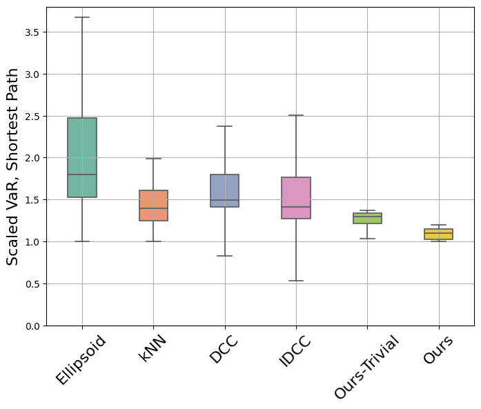
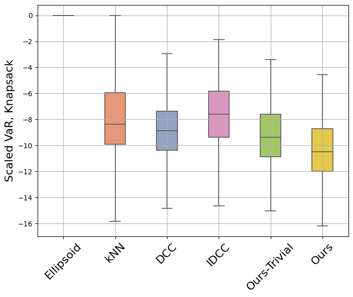
Refer to caption
Refer to caption
Figure 5: The scaled VaR for the objective in the shortest path and fractional knapsack problems. The x-axis lists the algorithms we test. The “Ellipsoid”, “kNN”, “DCC” and “IDCC” algorithms are introduced in the experiment descriptions. “Ours-Trivial” implements our algorithm but uses a trivial density ratio estimator w^1^𝑤1\hat{w}\equiv 1. “Ours” implements our algorithm and uses the probabilistic classification method to estimate w^^𝑤\hat{w}. Amongst the benchmark algorithms, our proposed Algorithm 1 generally achieves the lowest VaR.

Appendix D Proof of Theorems

D.1 Proof of Theorem 1

Let N|𝒟2|𝑁subscript𝒟2N\coloneqq|\mathcal{D}_{2}| and define xi(ci,zi)subscript𝑥𝑖subscript𝑐𝑖subscript𝑧𝑖x_{i}\coloneqq(c_{i},z_{i}) for i=1,,N𝑖1𝑁i=1,\ldots,N. The final η𝜂\eta term produced from Algorithm 1 is a function of (x1,,xN)subscript𝑥1subscript𝑥𝑁(x_{1},\ldots,x_{N}), which we define below as the η^()^𝜂\hat{\eta}(\cdot) function

η^(x1,,xN)min{η0:i=1Nw(xi)𝟙{|f^(zi)ci|ηh^(zi)}αi=1Nw(xi)}.^𝜂subscript𝑥1subscript𝑥𝑁:𝜂0superscriptsubscript𝑖1𝑁𝑤subscript𝑥𝑖1^𝑓subscript𝑧𝑖subscript𝑐𝑖𝜂^subscript𝑧𝑖𝛼superscriptsubscript𝑖1𝑁𝑤subscript𝑥𝑖\hat{\eta}(x_{1},\ldots,x_{N})\coloneqq\min\left\{\eta\geq 0\ :\ \sum_{i=1}^{N}w(x_{i})\cdot\mathbbm{1}\{|\hat{f}(z_{i})-c_{i}|\leq\eta\cdot\hat{h}(z_{i})\}\geq\alpha\cdot\sum_{i=1}^{N}w(x_{i})\right\}.

For each xisubscript𝑥𝑖x_{i}, let η~(xi)~𝜂subscript𝑥𝑖\tilde{\eta}(x_{i}) denote the minimum η𝜂\eta such that [f^(zi)ηh^(zi),f^(zi)+ηh^(zi)]^𝑓subscript𝑧𝑖𝜂^subscript𝑧𝑖^𝑓subscript𝑧𝑖𝜂^subscript𝑧𝑖[\hat{f}(z_{i})-\eta\cdot\hat{h}(z_{i}),\hat{f}(z_{i})+\eta\cdot\hat{h}(z_{i})] covers cisubscript𝑐𝑖c_{i}. The η~()~𝜂\tilde{\eta}(\cdot) function is formally defined below

η~(xi)min{η0:|f^(zi)ci|ηh^(zi)}.~𝜂subscript𝑥𝑖:𝜂0^𝑓subscript𝑧𝑖subscript𝑐𝑖𝜂^subscript𝑧𝑖\tilde{\eta}(x_{i})\coloneqq\min\left\{\eta\geq 0\ :\ |\hat{f}(z_{i})-c_{i}|\leq\eta\cdot\hat{h}(z_{i})\right\}.

Under this new notation, the form of η^()^𝜂\hat{\eta}(\cdot) can be formulated as

η^(x1,,xN)=min{η0:i=1Nw(xi)𝟙{ηη~(xi)}αi=1Nw(xi)}.^𝜂subscript𝑥1subscript𝑥𝑁:𝜂0superscriptsubscript𝑖1𝑁𝑤subscript𝑥𝑖1𝜂~𝜂subscript𝑥𝑖𝛼superscriptsubscript𝑖1𝑁𝑤subscript𝑥𝑖\hat{\eta}(x_{1},\ldots,x_{N})=\min\left\{\eta\geq 0\ :\ \sum_{i=1}^{N}w(x_{i})\cdot\mathbbm{1}\{\eta\geq\tilde{\eta}(x_{i})\}\geq\alpha\cdot\sum_{i=1}^{N}w(x_{i})\right\}.

Further, if the density ratio estimate in Algorithm 1 is perfect, then the event {cnew𝒰α(znew)}subscript𝑐newsubscript𝒰𝛼subscript𝑧new\{c_{\mathrm{new}}\in\mathcal{U}_{\alpha}(z_{\mathrm{new}})\} is equivent to {η~(xnew)η^(x1,,xN)}~𝜂subscript𝑥new^𝜂subscript𝑥1subscript𝑥𝑁\{\tilde{\eta}(x_{\mathrm{new}})\leq\hat{\eta}(x_{1},\ldots,x_{N})\}. We restate Theorem 1 below and provide a proof.

Theorem D.1.

Under Assumption 1, suppose the density ratio estimate is perfect, i.e., w^(c,z)=w(c,z)=q(c,z)/p(c,z)^𝑤𝑐𝑧𝑤𝑐𝑧𝑞𝑐𝑧𝑝𝑐𝑧\hat{w}(c,z)=w(c,z)=q(c,z)/p(c,z), then the uncertainty set 𝒰α(z)subscript𝒰𝛼𝑧\mathcal{U}_{\alpha}(z) generated by Algorithm 1 satisfies the following coverage guarantee,

|(η~(xnew)η^(x1,,xN))α|1N+1w¯w¯~𝜂subscript𝑥new^𝜂subscript𝑥1subscript𝑥𝑁𝛼1𝑁1¯𝑤¯𝑤\Big{|}\mathbb{P}\left(\tilde{\eta}(x_{\mathrm{new}})\leq\hat{\eta}(x_{1},\ldots,x_{N})\right)-\alpha\Big{|}\leq\dfrac{1}{N+1}\cdot\dfrac{\bar{w}}{\underline{w}}

where the probability on the left-hand-side is with respect to xnew𝒬similar-tosubscript𝑥new𝒬x_{\mathrm{new}}\sim\mathcal{Q} and x1,,xN𝒫similar-tosubscript𝑥1subscript𝑥𝑁𝒫x_{1},\ldots,x_{N}\sim\mathcal{P}.

Proof.

Since the distributions 𝒫𝒫\mathcal{P} and 𝒬𝒬\mathcal{Q} are continuous, almost surely the samples x1,,xN,xnewsubscript𝑥1subscript𝑥𝑁subscript𝑥newx_{1},\ldots,x_{N},x_{\mathrm{new}} are mutually distinct. Let {}\{\cdot\} denote an unordered set (e.g. {x1,,xN}subscript𝑥1subscript𝑥𝑁\{x_{1},\ldots,x_{N}\} denotes an unordered set containing distinct elements x1,,xNsubscript𝑥1subscript𝑥𝑁x_{1},\ldots,x_{N}). Then the following equation holds:

(η~(xnew)η^(x1,,xN))~𝜂subscript𝑥new^𝜂subscript𝑥1subscript𝑥𝑁\displaystyle\mathbb{P}(\tilde{\eta}(x_{\mathrm{new}})\leq\hat{\eta}(x_{1},\ldots,x_{N})) (21)
={a1,,aN+1}(η~(xnew)η^(x1,,xN)|{x1,,xn,xnew}={a1,,aN+1})absentsubscriptsubscript𝑎1subscript𝑎𝑁1~𝜂subscript𝑥newconditional^𝜂subscript𝑥1subscript𝑥𝑁subscript𝑥1subscript𝑥𝑛subscript𝑥newsubscript𝑎1subscript𝑎𝑁1\displaystyle=\int_{\{a_{1},\ldots,a_{N+1}\}}\mathbb{P}\bigg{(}\tilde{\eta}(x_{\mathrm{new}})\leq\hat{\eta}(x_{1},\ldots,x_{N})\ \bigg{|}\ \{x_{1},\ldots,x_{n},x_{\mathrm{new}}\}=\{a_{1},\ldots,a_{N+1}\}\bigg{)}
({x1,,xn,xnew}={a1,,aN+1}).absentsubscript𝑥1subscript𝑥𝑛subscript𝑥newsubscript𝑎1subscript𝑎𝑁1\displaystyle\phantom{=\int_{\{a_{1},\ldots,a_{N+1}\}}}\cdot\mathbb{P}\bigg{(}\{x_{1},\ldots,x_{n},x_{\mathrm{new}}\}=\{a_{1},\ldots,a_{N+1}\}\bigg{)}.

The integration is over all possible sets of N+1𝑁1N+1 distinct elements, denoted by {a1,,aN+1}subscript𝑎1subscript𝑎𝑁1\{a_{1},\ldots,a_{N+1}\}. The remaining part of the proof uniformly bounds the (η~(xnew)η^(x1,,xN)|{x1,,xn,xnew}={a1,,aN+1})~𝜂subscript𝑥newconditional^𝜂subscript𝑥1subscript𝑥𝑁subscript𝑥1subscript𝑥𝑛subscript𝑥newsubscript𝑎1subscript𝑎𝑁1\mathbb{P}\bigg{(}\tilde{\eta}(x_{\mathrm{new}})\leq\hat{\eta}(x_{1},\ldots,x_{N})\ \bigg{|}\ \{x_{1},\ldots,x_{n},x_{\mathrm{new}}\}=\{a_{1},\ldots,a_{N+1}\}\bigg{)} term for all sets {a1,,aN+1}subscript𝑎1subscript𝑎𝑁1\{a_{1},\ldots,a_{N+1}\}.

Given a set {a1,,aN+1}subscript𝑎1subscript𝑎𝑁1\{a_{1},\ldots,a_{N+1}\}, let E𝐸E denote the event that {x1,,xn,xnew}={a1,,aN+1}subscript𝑥1subscript𝑥𝑛subscript𝑥newsubscript𝑎1subscript𝑎𝑁1\{x_{1},\ldots,x_{n},x_{\mathrm{new}}\}=\{a_{1},\ldots,a_{N+1}\}, and let Eisubscript𝐸𝑖E_{i} denote the event that xnew=aisubscript𝑥newsubscript𝑎𝑖x_{\mathrm{new}}=a_{i} and {x1,,xN}={a1,,aN+1}\{ai}subscript𝑥1subscript𝑥𝑁\subscript𝑎1subscript𝑎𝑁1subscript𝑎𝑖\{x_{1},\ldots,x_{N}\}=\{a_{1},\ldots,a_{N+1}\}\backslash\{a_{i}\}. The (η~(xnew)η^(x1,,xN)|E)~𝜂subscript𝑥newconditional^𝜂subscript𝑥1subscript𝑥𝑁𝐸\mathbb{P}\bigg{(}\tilde{\eta}(x_{\mathrm{new}})\leq\hat{\eta}(x_{1},\ldots,x_{N})\ \bigg{|}\ E\bigg{)} term can be decomposed by the following chain of equations:

(η~(xnew)η^(x1,,xN)|E)~𝜂subscript𝑥newconditional^𝜂subscript𝑥1subscript𝑥𝑁𝐸\displaystyle\mathbb{P}\bigg{(}\tilde{\eta}(x_{\mathrm{new}})\leq\hat{\eta}(x_{1},\ldots,x_{N})\ \bigg{|}\ E\bigg{)} (22)
=i=1N+1(EiE)(η~(xnew)η^(x1,,xN)|Ei)absentsuperscriptsubscript𝑖1𝑁1conditionalsubscript𝐸𝑖𝐸~𝜂subscript𝑥newconditional^𝜂subscript𝑥1subscript𝑥𝑁subscript𝐸𝑖\displaystyle=\sum_{i=1}^{N+1}\mathbb{P}(E_{i}\mid E)\cdot\mathbb{P}\bigg{(}\tilde{\eta}(x_{\mathrm{new}})\leq\hat{\eta}(x_{1},\ldots,x_{N})\ \bigg{|}\ E_{i}\bigg{)}
=(1)i=1N+1(EiE)𝟙{η~(xnew)η^(x1,,xN)|Ei}superscript1absentsuperscriptsubscript𝑖1𝑁1conditionalsubscript𝐸𝑖𝐸1conditional-set~𝜂subscript𝑥new^𝜂subscript𝑥1subscript𝑥𝑁subscript𝐸𝑖\displaystyle\stackrel{{\scriptstyle(1)}}{{=}}\sum_{i=1}^{N+1}\mathbb{P}(E_{i}\mid E)\cdot\mathbbm{1}\bigg{\{}\tilde{\eta}(x_{\mathrm{new}})\leq\hat{\eta}(x_{1},\ldots,x_{N})\ \bigg{|}\ E_{i}\bigg{\}}
=(2)i=1N+1w(ai)j=1N+1w(aj)𝟙{η~(xnew)η^(x1,,xN)|Ei},superscript2absentsuperscriptsubscript𝑖1𝑁1𝑤subscript𝑎𝑖superscriptsubscript𝑗1𝑁1𝑤subscript𝑎𝑗1conditional-set~𝜂subscript𝑥new^𝜂subscript𝑥1subscript𝑥𝑁subscript𝐸𝑖\displaystyle\stackrel{{\scriptstyle(2)}}{{=}}\sum_{i=1}^{N+1}\dfrac{w(a_{i})}{\sum_{j=1}^{N+1}w(a_{j})}\cdot\mathbbm{1}\bigg{\{}\tilde{\eta}(x_{\mathrm{new}})\leq\hat{\eta}(x_{1},\ldots,x_{N})\ \bigg{|}\ E_{i}\bigg{\}},

where (1)1(1) is from the fact that η^(x1,,xN)^𝜂subscript𝑥1subscript𝑥𝑁\hat{\eta}(x_{1},\ldots,x_{N}) is invariant to the permutation of (x1,,xN)subscript𝑥1subscript𝑥𝑁(x_{1},\ldots,x_{N}), and (2)2(2) is by that

(Ei)subscript𝐸𝑖\displaystyle\mathbb{P}(E_{i}) =N!q(ai)jip(aj)absent𝑁𝑞subscript𝑎𝑖subscriptproduct𝑗𝑖𝑝subscript𝑎𝑗\displaystyle=N!\cdot q(a_{i})\cdot\prod_{j\neq i}p(a_{j})
=N!w(ai)j=1N+1p(aj),absent𝑁𝑤subscript𝑎𝑖superscriptsubscriptproduct𝑗1𝑁1𝑝subscript𝑎𝑗\displaystyle=N!\cdot w(a_{i})\cdot\prod_{j=1}^{N+1}p(a_{j}),

and (E)=i=1N+1(Ei)𝐸superscriptsubscript𝑖1𝑁1subscript𝐸𝑖\mathbb{P}(E)=\sum_{i=1}^{N+1}\mathbb{P}(E_{i}).

We now characterize the terms 𝟙{η~(xnew)η^(x1,,xN)|Ei}1conditional-set~𝜂subscript𝑥new^𝜂subscript𝑥1subscript𝑥𝑁subscript𝐸𝑖\mathbbm{1}\bigg{\{}\tilde{\eta}(x_{\mathrm{new}})\leq\hat{\eta}(x_{1},\ldots,x_{N})\ \bigg{|}\ E_{i}\bigg{\}}. Without loss of generality, let η~(a1)<η~(a2)<η~(aN+1)~𝜂subscript𝑎1~𝜂subscript𝑎2~𝜂subscript𝑎𝑁1\tilde{\eta}(a_{1})<\tilde{\eta}(a_{2})\cdots<\tilde{\eta}(a_{N+1}), then

𝟙{η~(xnew)η^(x1,,xN)|Ei}1conditional-set~𝜂subscript𝑥new^𝜂subscript𝑥1subscript𝑥𝑁subscript𝐸𝑖\displaystyle\mathbbm{1}\bigg{\{}\tilde{\eta}(x_{\mathrm{new}})\leq\hat{\eta}(x_{1},\ldots,x_{N})\ \bigg{|}\ E_{i}\bigg{\}} (23)
=𝟙{η~(ai)η^({a1,,aN+1}\{ai})}absent1~𝜂subscript𝑎𝑖^𝜂\subscript𝑎1subscript𝑎𝑁1subscript𝑎𝑖\displaystyle=\mathbbm{1}\bigg{\{}\tilde{\eta}(a_{i})\leq\hat{\eta}(\{a_{1},\ldots,a_{N+1}\}\backslash\{a_{i}\})\bigg{\}}
=𝟙{j=1i1w(aj)<αjiw(aj)}.absent1superscriptsubscript𝑗1𝑖1𝑤subscript𝑎𝑗𝛼subscript𝑗𝑖𝑤subscript𝑎𝑗\displaystyle=\mathbbm{1}\bigg{\{}\sum_{j=1}^{i-1}w(a_{j})<\alpha\cdot\sum_{j\neq i}w(a_{j})\bigg{\}}.

The last line of (23) has the following bounds:

𝟙{j=1iw(aj)<αj=1N+1w(aj)}𝟙{j=1i1w(aj)<αjiw(aj)}𝟙{j=1i1w(aj)<αj=1N+1w(aj)}.1superscriptsubscript𝑗1𝑖𝑤subscript𝑎𝑗𝛼superscriptsubscript𝑗1𝑁1𝑤subscript𝑎𝑗1superscriptsubscript𝑗1𝑖1𝑤subscript𝑎𝑗𝛼subscript𝑗𝑖𝑤subscript𝑎𝑗1superscriptsubscript𝑗1𝑖1𝑤subscript𝑎𝑗𝛼superscriptsubscript𝑗1𝑁1𝑤subscript𝑎𝑗\mathbbm{1}\bigg{\{}\sum_{j=1}^{i}w(a_{j})<\alpha\cdot\sum_{j=1}^{N+1}w(a_{j})\bigg{\}}\leq\mathbbm{1}\bigg{\{}\sum_{j=1}^{i-1}w(a_{j})<\alpha\cdot\sum_{j\neq i}w(a_{j})\bigg{\}}\leq\mathbbm{1}\bigg{\{}\sum_{j=1}^{i-1}w(a_{j})<\alpha\cdot\sum_{j=1}^{N+1}w(a_{j})\bigg{\}}. (24)

Combining (22), (23) and (24), the (η~(xnew)η^(x1,,xN)|{x1,,xn,xnew}={a1,,aN+1})~𝜂subscript𝑥newconditional^𝜂subscript𝑥1subscript𝑥𝑁subscript𝑥1subscript𝑥𝑛subscript𝑥newsubscript𝑎1subscript𝑎𝑁1\mathbb{P}\bigg{(}\tilde{\eta}(x_{\mathrm{new}})\leq\hat{\eta}(x_{1},\ldots,x_{N})\ \bigg{|}\ \{x_{1},\ldots,x_{n},x_{\mathrm{new}}\}=\{a_{1},\ldots,a_{N+1}\}\bigg{)} term is uniformly bounded:

(η~(xnew)η^(x1,,xN)|E)~𝜂subscript𝑥newconditional^𝜂subscript𝑥1subscript𝑥𝑁𝐸\displaystyle\mathbb{P}\bigg{(}\tilde{\eta}(x_{\mathrm{new}})\leq\hat{\eta}(x_{1},\ldots,x_{N})\ \bigg{|}\ E\bigg{)}
i=1N+1w(ai)j=1N+1w(aj)𝟙{j=1iw(aj)<αj=1N+1w(aj)}absentsuperscriptsubscript𝑖1𝑁1𝑤subscript𝑎𝑖superscriptsubscript𝑗1𝑁1𝑤subscript𝑎𝑗1superscriptsubscript𝑗1𝑖𝑤subscript𝑎𝑗𝛼superscriptsubscript𝑗1𝑁1𝑤subscript𝑎𝑗\displaystyle\geq\sum_{i=1}^{N+1}\dfrac{w(a_{i})}{\sum_{j=1}^{N+1}w(a_{j})}\cdot\mathbbm{1}\bigg{\{}\sum_{j=1}^{i}w(a_{j})<\alpha\cdot\sum_{j=1}^{N+1}w(a_{j})\bigg{\}}
αw¯j=1N+1w(aj)α1N+1w¯w¯.absent𝛼¯𝑤superscriptsubscript𝑗1𝑁1𝑤subscript𝑎𝑗𝛼1𝑁1¯𝑤¯𝑤\displaystyle\geq\alpha-\dfrac{\bar{w}}{\sum_{j=1}^{N+1}w(a_{j})}\geq\alpha-\dfrac{1}{N+1}\cdot\dfrac{\bar{w}}{\underline{w}}.
(η~(xnew)η^(x1,,xN)|E)~𝜂subscript𝑥newconditional^𝜂subscript𝑥1subscript𝑥𝑁𝐸\displaystyle\mathbb{P}\bigg{(}\tilde{\eta}(x_{\mathrm{new}})\leq\hat{\eta}(x_{1},\ldots,x_{N})\ \bigg{|}\ E\bigg{)}
i=1N+1w(ai)j=1N+1w(aj)𝟙{j=1i1w(aj)<αj=1N+1w(aj)}absentsuperscriptsubscript𝑖1𝑁1𝑤subscript𝑎𝑖superscriptsubscript𝑗1𝑁1𝑤subscript𝑎𝑗1superscriptsubscript𝑗1𝑖1𝑤subscript𝑎𝑗𝛼superscriptsubscript𝑗1𝑁1𝑤subscript𝑎𝑗\displaystyle\leq\sum_{i=1}^{N+1}\dfrac{w(a_{i})}{\sum_{j=1}^{N+1}w(a_{j})}\cdot\mathbbm{1}\bigg{\{}\sum_{j=1}^{i-1}w(a_{j})<\alpha\cdot\sum_{j=1}^{N+1}w(a_{j})\bigg{\}}
α+w¯j=1N+1w(aj)α+1N+1w¯w¯.absent𝛼¯𝑤superscriptsubscript𝑗1𝑁1𝑤subscript𝑎𝑗𝛼1𝑁1¯𝑤¯𝑤\displaystyle\leq\alpha+\dfrac{\bar{w}}{\sum_{j=1}^{N+1}w(a_{j})}\leq\alpha+\dfrac{1}{N+1}\cdot\dfrac{\bar{w}}{\underline{w}}.

Plugging the bounds above into (21) finishes the proof.

D.2 Proof of Corollary 1

By defining the estimated test distribution 𝒬^^𝒬\hat{\mathcal{Q}} as a distribution with the following density function:

q^(c,z)=w^(c,z)p(c,z)(c,z)w^(c,z)p(c,z)dzdc,^𝑞𝑐𝑧^𝑤𝑐𝑧𝑝𝑐𝑧subscript𝑐𝑧^𝑤𝑐𝑧𝑝𝑐𝑧differential-d𝑧differential-d𝑐\hat{q}(c,z)=\dfrac{\hat{w}(c,z)\cdot p(c,z)}{\int_{(c,z)}\hat{w}(c,z)\cdot p(c,z)\mathrm{d}z\mathrm{d}c},

we could directly apply Theorem 1 to see that

|𝒬^(cnew𝒰α(znew))α|1|𝒟2|+1w¯w¯,subscript^𝒬subscript𝑐newsubscript𝒰𝛼subscript𝑧new𝛼1subscript𝒟21¯𝑤¯𝑤\Big{|}\mathbb{P}_{\hat{\mathcal{Q}}}\left(c_{\mathrm{new}}\in\mathcal{U}_{\alpha}(z_{\mathrm{new}})\right)-\alpha\Big{|}\leq\dfrac{1}{|\mathcal{D}_{2}|+1}\cdot\dfrac{\bar{w}}{\underline{w}}, (25)

where the probability 𝒬^subscript^𝒬\mathbb{P}_{\hat{\mathcal{Q}}} is with respect to (cnew,znew)𝒬^similar-tosubscript𝑐newsubscript𝑧new^𝒬(c_{\text{new}},z_{\text{new}})\sim\hat{\mathcal{Q}} and 𝒟2𝒫similar-tosubscript𝒟2𝒫\mathcal{D}_{2}\sim\mathcal{P}. From the definition of the total variation distance, the following inequality holds:

|𝒬^(cnew𝒰α(znew))(cnew𝒰α(znew))|DTV(𝒬,𝒬^),subscript^𝒬subscript𝑐newsubscript𝒰𝛼subscript𝑧newsubscript𝑐newsubscript𝒰𝛼subscript𝑧newsubscript𝐷TV𝒬^𝒬\Big{|}\mathbb{P}_{\hat{\mathcal{Q}}}\left(c_{\mathrm{new}}\in\mathcal{U}_{\alpha}(z_{\mathrm{new}})\right)-\mathbb{P}\left(c_{\mathrm{new}}\in\mathcal{U}_{\alpha}(z_{\mathrm{new}})\right)\Big{|}\leq D_{\text{TV}}(\mathcal{Q},\hat{\mathcal{Q}}), (26)

where \mathbb{P} is with respect to (cnew,znew)𝒬similar-tosubscript𝑐newsubscript𝑧new𝒬(c_{\text{new}},z_{\text{new}})\sim\mathcal{Q} and 𝒟2𝒫similar-tosubscript𝒟2𝒫\mathcal{D}_{2}\sim\mathcal{P}. Combining (25) and (26) gives the result of Corollary 1, which we restate below:

|(cnew𝒰α(znew))α|1|𝒟2|+1w¯w¯+DTV(𝒬,𝒬^).subscript𝑐newsubscript𝒰𝛼subscript𝑧new𝛼1subscript𝒟21¯𝑤¯𝑤subscript𝐷TV𝒬^𝒬\Big{|}\mathbb{P}\left(c_{\mathrm{new}}\in\mathcal{U}_{\alpha}(z_{\mathrm{new}})\right)-\alpha\Big{|}\leq\dfrac{1}{|\mathcal{D}_{2}|+1}\cdot\dfrac{\bar{w}}{\underline{w}}+D_{\mathrm{TV}}(\mathcal{Q},\hat{\mathcal{Q}}).