A Localized Orthogonal Decomposition Method for Heterogeneous Stokes Problems
Abstract.
In this paper, we propose a multiscale method for heterogeneous Stokes problems. The method is based on the Localized Orthogonal Decomposition (LOD) methodology and has approximation properties independent of the regularity of the coefficients. We apply the LOD to an appropriate reformulation of the Stokes problem, which allows us to construct exponentially decaying basis functions for the velocity approximation while using a piecewise constant pressure approximation. The exponential decay motivates a localization of the basis computation, which is essential for the practical realization of the method. We perform a rigorous a priori error analysis and prove optimal convergence rates for the velocity approximation and a post-processed pressure approximation, provided that the supports of the basis functions are logarithmically increased with the desired accuracy. Numerical experiments support the theoretical results of this paper.
Key words and phrases:
Stokes problem, flow around obstacles, multiscale method, a priori error analysis, exponential decay1991 Mathematics Subject Classification:
65N12, 65N15, 65N30, 76D071. Introduction
This paper considers a heterogeneous Stokes problem posed in a bounded Lipschitz polytope , , which we assume to be of unit size. Given an external force , it seeks a velocity and a pressure such that
| (1.1) |
holds, where the coefficients and encode the heterogeneity of the problem. They may possibly be rough and involve oscillations on multiple non-separated length scales. Such problems may arise, for example, as part of more complex coupled problems where the viscosity is an unknown. A specific example is magma modeling, where the temperature-dependent viscosity can exhibit large spatial variations, cf. [20]. Problems like 1.1 can also be used as approximations to (slow) flow problems around numerous obstacles of possibly small diameter, cf. [1]. In this case, one sets as the physical viscosity and to zero in the fluid domain, while assigning large values to these coefficients inside the obstacles.
The numerical treatment of such heterogeneous problems with classical finite element methods (FEMs) suffers from suboptimal approximation rates and preasymptotic effects on meshes that do not resolve the coefficients. Since globally resolving all microscopic details of the coefficients may not be computationally feasible, we aim to construct a numerical method with reasonable errors already on coarse meshes. For diffusion-type problems, there is a whole zoo of multiscale methods that use coarse problem-adapted ansatz spaces. Two classes of methods may be distinguished: First, methods that exploit structural properties of the coefficients, such as periodicity and scale separation, to construct the problem-adapted basis functions. Their computational cost differs from that of classical FEMs on the same mesh only by the cost of solving a fixed number of local problems. This class includes the Heterogeneous Multiscale Method [14], the Two-Scale FEM [35], and the Multiscale FEM [24]. In contrast, methods in the second class achieve optimal approximation orders under minimal structural assumptions on the coefficients. This is achieved at the expense of a moderate computational overhead compared to classical FEMs. This overhead manifests itself in an enlarged support of the basis functions or an increased number of basis functions per mesh entity. Prominent methods for diffusion-type multiscale problems include the Generalized Multiscale FEM [16, 10], the Multiscale Spectral Generalized FEM (MS-GFEM) [9, 36], Adaptive Local Bases [19], the (Super-) Localized Orthogonal Decomposition (LOD) method [33, 21, 23], or Gamblets [37]; see also the review article [2]. We mention that the LOD and the MS-GFEM have been applied to Darcy-type problems, cf. [31, 3], which is also of mixed form but different in nature than the Stokes problem; see also [29].
Some of the methods of the first class have been successfully generalized to heterogeneous Stokes problems. For example, a homogenization-based method has been proposed in [8, 7] for slowly varying perforated media. As for the Multiscale FEM, its Crouzeix–Raviart version, first proposed in [28], has been applied to the Stokes problem in perforated domains in [32, 25, 17, 4]. The weak notion of continuity of the Crouzeix–Raviart method and an appropriate choice of the problem-adapted approximation space make it flexible enough to cope with the divergence-free constraint of the Stokes problem. On the contrary, we are not aware of any multiscale method for heterogeneous Stokes problems that works under the minimal structural assumptions on the coefficients.
This open question is addressed in this paper by adapting the LOD methodology to heterogeneous Stokes problems. The basic idea of the LOD is to decompose the solution space into a fine-scale space and its orthogonal complement with respect to the energy inner product induced by the considered problem. By choosing the fine-scale space to consist of functions that average out on coarse scales, one obtains a finite-dimensional mesh-based complement space that is adapted to the problem at hand and has uniform approximation properties under minimal structural assumptions on the coefficients. It possesses exponentially decaying basis functions whose computation can thus be localized to subdomains, resulting in a practically feasible method. For Stokes problems, the divergence-free constraint poses a major challenge to LOD-type methods, since directly incorporating the constraint can lead to ill-posed problems or slowly decaying basis functions. To overcome this problem, we reformulate the Stokes problem using the space of -functions, whose divergence is piecewise constant with respect to some coarse mesh, as the solution space for the velocity. The divergence-free velocity is then recovered using a piecewise constant Lagrange multiplier defined on the same mesh. Inspired by the Crouzeix–Raviart Multiscale FEM mentioned above, we then choose the fine-scale space for the velocity as the functions whose averages vanish on all faces of the coarse mesh. We prove that the finite-dimensional orthogonal complement possesses exponentially decaying basis functions, which paves the way to the construction of an LOD-type multiscale method. The use of face averages to define the fine-scale space is novel in the LOD context and allows us to construct the velocity approximation space independent of the pressure. The approximation of the resulting LOD method is exactly divergence-free and thus pressure robust in the sense of [26]. We also perform an a priori error analysis of the proposed method and prove optimal orders of convergence as the mesh size is decreased, provided that the support of the basis functions is allowed to increase logarithmically with the desired accuracy. More specifically, for -right-hand sides we prove first- and second-order convergence for the - and -errors of the velocity approximation, respectively, and first-order convergence for a post-processed pressure approximation. If the right-hand side is -regular, we can squeeze out an additional order of convergence for the velocity approximation. We emphasize that only minimal structural assumptions on the coefficients are necessary for this error analysis.
The paper is organized as follows: In Section 2 we introduce the model problem and a prototypical multiscale method is presented in Section 3. We prove the exponential decay of the prototypical basis functions and localize the basis computation in Section 4. A practical multiscale method is then presented in Section 5. Numerical experiments supporting our theoretical results are given in Section 6.
2. Model problem
This section introduces the weak formulation of the heterogeneous Stokes problem, along with classical results guaranteeing its well-posedness. The weak formulation is based on the Sobolev space endowed with homogeneous Dirichlet boundary conditions on and the space satisfying an integral-mean-zero constraint. In the following, we will always assume that there exist constants and such that
| (2.1) |
holds almost everywhere in . Denoting by the -inner product, the problem’s bilinear forms and are defined as
Given a source term , the weak formulation of the considered heterogeneous Stokes problem seeks a pair such that
| (2.2a) | ||||||||
| (2.2b) | ||||||||
holds for all .
Using the uniform coefficient bounds 2.1 one can show that the bilinear form is continuous and coercive, i.e., there exist constants such that
| (2.3) |
holds for all , where denotes the -norm. Note that by the Poincaré–Friedrichs inequality, the seminorm is equivalent to the full -norm. The constants in 2.3 can be specified as and , where denotes the Poincaré–Friedrichs constant.
To establish the well-posedness of problem 2.2, we need a compatibility condition between the spaces and , expressed as the inf–sup condition
| (2.4) |
where is typically called the inf–sup constant. This condition is classical and it is typically proved using the so-called Ladyzhenskaya lemma, cf. [27]. It states that for any there exists such that
| (2.5) |
which directly implies the inf–sup stability with inf–sup constant . After establishing conditions 2.3 and 2.4, the well-posedness of weak formulation 2.2 can be concluded using classical inf–sup theory; see, e.g., [5].
3. Prototypical multiscale method
This section introduces a prototypical multiscale method that achieves optimal order approximations without preasymptotic effects under minimal structural assumptions on the coefficients. To this end, we introduce a geometrically conforming, quasi-uniform, and shape-regular hierarchy of simplicial111One can also use general polygonal/polyhedral meshes. We assume that the meshes are simplicial only to simplify the presentation. The method itself can be applied to more general meshes in a straightforward manner. An extension to meshes with curved elements is also possible. meshes . Each mesh is a finite subdivision of the closure of , into closed elements , which are -dimensional simplices. The parameter denotes the mesh size and is defined as the maximum diameter of the elements in , i.e., . We further denote the space of -piecewise constant functions by and write for the corresponding -orthogonal projection. The set of all faces of the mesh is denoted by and the subset of interior faces by .
For the construction of the prototypical multiscale method we will use an equivalent reformulation of problem 2.2. This reformulation is based on the spaces
| (3.1) |
where the space partially integrates the divergence-free constraint into the velocity space. Thus, the smaller space is sufficient to enforce that the velocity is divergence-free. The reformulation seeks such that
| (3.2a) | ||||||||
| (3.2b) | ||||||||
holds for all . To prove the well-posedness of this reformulated problem we verify the corresponding inf–sup condition. This inf–sup condition can be shown to hold with the constant from 2.4, using again the Ladyzhenskaya lemma, cf. 2.5. It is easy to verify that the first component of the solution to the reformulated problem coincides with the velocity from 2.2 and that for the second component we have , where is the pressure from 2.2.
Following the construction of the LOD for diffusion-type problems, cf. [33, 34], we consider a decomposition of the space into the direct sum of two subspaces. The first one, typically referred to as fine-scale space, contains functions that average out on coarse scales and is defined as
| (3.3) |
The second subspace is finite-dimensional and will serve as the approximation space of the prototypical LOD method. It is defined as the orthogonal complement of with respect to the energy inner product , i.e.,
| (3.4) |
Note that, since is constructed as the orthogonal complement of with respect to the problem-dependent inner product , it contains problem-specific information that allows reliable approximations even at coarse scales. The use of tildes in the notation of functions and spaces is intended to emphasize that they are adapted to the problem at hand. The following lemma constructs a basis of the space .
Lemma 3.1 (Prototypical basis).
The space has dimension with denoting the number of interior faces, and a basis of it is given by
| (3.5) |
with defined for all and as the unique solutions to: seek with such that
| (3.6a) | ||||||||||
| (3.6b) | ||||||||||
| (3.6c) | ||||||||||
holds for all . Here, we label the entries of a vector using face-index pairs as , and the bilinear form is defined as
where denotes the canonical basis of .
Before proving this lemma, we introduce some technical tools that will be used not only in its proof, but also on several other occasions in the remainder of this paper. First, we note that the Ladyzhenskaya lemma stated in 2.5 for the whole domain also holds locally on elements . More precisely, there exists a constant such that, for every element and all functions with , there exists such that
| (3.7) |
holds, where the constant depends only on the shape regularity of the mesh. The latter statement can be inferred, for example, from [6], where the shape-dependence of the Ladyzhenskaya constant is investigated. The locally supported functions from 3.7, hereafter referred to as element bubble functions, will be frequently used to estimate the bilinear form .
Furthermore, for estimating the bilinear form , we introduce face bubble functions denoted by . Each bubble function is locally supported with , where is the union of the two elements that share face . The edge bubbles are chosen such that holds for all and , and the two stability estimates
| (3.8) |
are satisfied for a constant independent of . Additionally, we demand that the divergence of the edge bubbles is piecewise constant, i.e., . Note that bubbles with these properties can be constructed using classical edge bubbles, which we denote by below, cf. [39]. They satisfy for any . We then define , where is supported on and defined locally on as the -function satisfying , where denotes the unit normal on outward of . The function exist thanks to (3.7) and satisfies .
Now let us proceed with the proof of the lemma above.
Proof of Lemma 3.1.
We first prove the well-posedness of problem 3.6. To this end, we verify the inf–sup stability of the bilinear form defined as , i.e., there exists a constant such that
| (3.9) |
holds, where with denoting the Euclidean norm.
Given any , we choose a function defined as
where, for any , satisfies locally on as well as , cf. 3.7. By construction, it holds and we have for any that
where we used estimates 3.8 and 3.7. Summing over all elements gives
which proves inf–sup condition 3.9 with the constant , defined as the reciprocal of the constant in the estimate above.
Next, we prove that 3.5 constitutes a basis of the space . To this end, we first note that conditions 3.6a and 3.6b imply that for all and . To prove the basis property, we consider an arbitrary and set . Since and, at the same time, is -orthogonal to , it must hold that . Thus, any can be written as a unique linear combination of the linearly independent functions , which shows that they form a basis of the space . This concludes the proof. ∎
Having introduced the prototypical basis functions, we can define a projection operator which preserves face integrals for any by
| (3.10) |
This operator coincides with the -orthogonal projection onto , since for any and it holds that , noting that . This orthogonality property also implies the continuity of , i.e., for any it holds
| (3.11) |
where we used 2.3. Furthermore, applying the divergence theorem, using the fact that preserves face integrals, and noting that by the definition of functions in this space have a piecewise constant divergence, cf. 3.1, one can show that
| (3.12) |
holds for any and .
The desired prototypical method then seeks such that
| (3.13a) | ||||||||
| (3.13b) | ||||||||
holds for all . For the analysis of this method in the theorem below we need an approximation result for . Using the Poincaré inequality on convex domains, cf. [38], it hollows that for all and it holds
| (3.14) |
Theorem 3.2 (Prototypical method).
Proof.
First, we prove the inf–sup condition
| (3.17) |
for some constant , which implies the well-posedness of 3.13. Given any , we denote by the function with and , cf. 2.5, and define . One can show that using 3.12, and that by the continuity of , cf. 3.11, and the particular choice of . Combining these results, inf–sup condition 3.17 follows directly with the constant . Using that is -orthogonal, identity 3.12, as well as that solves 3.2, it is a straightforward observation that solves 3.13. The uniqueness of the solution to 3.13 then implies that and .
Second, we derive error estimates for the prototypical multiscale method. To this end, we note that the error is an element of the space . Furthermore, we have for all that , where we apply 3.12 to and note that . This implies that . Using the first estimate in 2.3, that , 3.2a with as test function, that , and the local Poincaré-type inequality from Lemma A.1, we obtain that
| (3.18) |
which implies the desired -error estimate for .
In the case , we add and subtract in 3.18, the projection of onto piecewise constants, which results in
| (3.19) |
where the first term on the right-hand side can be bounded using approximation result 3.14 and the Poincaré-type inequality from Lemma A.1 as
| (3.20) |
Abbreviating , the second term on the right-hand side of 3.19 can be locally rewritten using the divergence theorem and that as
| (3.21) |
Summing over all elements using that for all then gives
| (3.22) |
where we denote by the barycenter of and by the jump of a function across face chosen consistently with the fixed normal associated to .
To estimate the term on the right-hand side of the previous equation, we combine the approximation result of 3.14 with Lemma A.2, which gives for any and with that holds for any with and the constant . Applying this estimate to and , noting that and yields that
Combining 3.22 with the latter bounds and using the Cauchy–Schwarz inequality, we obtain for the second term on the right-hand side of 3.19 that
| (3.23) |
Inserting estimates 3.20 and 3.23 into 3.19 yields the desired -error estimate in the case that . Therefore, taking the maximum of the constants yields estimate 3.16 with .
We emphasize that squeezing out an additional order of convergence for -regular right-hand sides only works in the context of Stokes problems and not for diffusion-type problems. This observation can also be verified numerically.
4. Exponential decay and localization
We emphasize that the prototypical LOD basis functions defined in 3.5 are globally supported. Therefore, their computation would require the solution to global problems, which we consider infeasible. In this section, we show that the prototypical LOD basis functions decay exponentially, which motivates their approximation by locally computable counterparts. A practical multiscale method based on such local approximations is presented in Section 5.
To quantify the decay of the basis functions, we introduce the notion of patches with respect to the coarse mesh . Given an oversampling parameter , where denotes the (positive) natural numbers, we define the patch of order around a union of elements recursively by
| (4.1) |
and set . The notion of patches can also be extended to faces by defining, for any , the patch of order around by , where denotes the union of the two elements sharing the face . The following theorem proves the exponential decay of the prototypical LOD basis functions.
Theorem 4.1 (Exponential decay).
There exists a constant independent of , , , and such that for all , , and , it holds that
| (4.2) |
Proof.
In the following, we will use the abbreviation and consider a cut-off function with the properties
| (4.3) |
and the bound
| (4.4) |
where is a constant independent of .
Using as a test function in 3.6a gives that
which, using subscripts to denote the restrictions of the bilinear forms and to subdomains, can be rewritten as
| (4.5) |
Here, we dropped the subscript of and used that , that the divergence of is piecewise constant on , and that for all faces not inside . Using coefficient bound 2.1, we can estimate 4.5 as
| (4.6) | ||||
To estimate , we again use coefficient bound 2.1, the bound on from 4.4, and the Poincaré-type inequality from Lemma A.1 to get that
| (4.7) |
with the constant . Above we used that, for any element , there exists a face such that .
Using similar arguments, we obtain for that
| (4.8) |
To continue the latter estimate, we need a local bound for . To this end, we test 3.6a for any element with chosen such that holds locally in and is satisfied, cf. 3.7. This results in
| (4.9) |
Summing the latter bound over all elements with , we obtain an estimate for which can be inserted in 4.8 to conclude
To estimate , we apply the Cauchy–Schwarz inequality for all faces , where denotes the set of faces inside , which yields that
where denotes the -dimensional volume. We derive a bound for for all faces by testing 3.6a with the bubble function , which gives
| (4.10) |
Here, we used the second estimates of 2.3 and 3.8 and that since the divergence of is piecewise constant and has zero element averages.
Noting that , the latter estimate can be used to show that
where we applied the discrete Cauchy–Schwarz inequality. Using the trace inequality from Lemma A.2, we obtain that
Inserting the above estimates for , , and into 4.6 and noting that can be rewritten as , we obtain that
with the constant
As a direct consequence, we obtain that
which, after iterating, yields that
for the constant . This concludes the proof. ∎
Motivated by the exponential decay of the prototypical LOD basis functions defined in 3.5, we will introduce localizations of them. To formulate the corresponding problems, we introduce localized versions of the spaces and as
| (4.11) | ||||
Furthermore, we denote by the subspace consisting of vectors with for all faces not contained in the interior of the patch , where we recall that is a notation for the entries of the vector .
Given an oversampling parameter , the localized basis functions, denoted by
are determined by the problems: Seek such that
| (4.12a) | ||||||||||
| (4.12b) | ||||||||||
| (4.12c) | ||||||||||
holds for all . This saddle point problem is well-posed, which can be shown using similar arguments as in the proof of Lemma 3.1.
In the following, we will frequently use the bound
| (4.13) |
which can be proved by testing equation 4.12a first with and then with , and combining the resulting estimates.
With the localized basis functions at hand, we are now able to define a localized counterpart of the operator from 3.10. This operator, denoted by , is a projection onto the span of the localized basis functions with the property that it preserves face integrals. More precisely, it is for any defined as
| (4.14) |
We emphasize that, unlike , this projection is not -orthogonal.
The following theorem proves that approximates exponentially well. Note that using this result for the bubble function gives an exponential approximation result for the corresponding localized and prototypical basis functions.
Theorem 4.2 (Localization error).
There exist a constant independent of and such that for all and , it holds that
| (4.15) |
Proof.
We consider an arbitrary but fixed and abbreviate and , which allows us to write
| (4.16) |
using the definitions of and . Applying the first bound from 2.3 then gives
| (4.17) |
To estimate the terms on the right-hand side of the latter inequality, we fix a face and index and recall the definition of the cut-off function in 4.3, which we now denote by . Note that, by the definition of the space and since , it holds that . Using this and observing that is an admissible test function in equation (4.12a), we obtain that
| (4.18) | ||||
In the following, we estimate the terms , , and separately. To estimate , we note that the divergence of is piecewise constant on and that has zero element averages. This together with 4.4 and A.1 gives
| (4.19) |
To derive a -bound for , we proceed similarly as in 4.9, which yields that
and inserting this into 4.19 gives
To estimate , we apply the discrete Chauchy–Schwarz inequality, the trace inequality from Lemma A.2, the bound , and the local Poincaré-type inequality from Lemma A.1, which yields that
To derive a bound for , we proceed as in 4.10, but locally, which results in
Using this estimate, the above estimate for can be continued as
Inserting the above estimates for , , and into 4.18 gives the bound
with
We can now apply the exponential decay result of Theorem 4.1 to instead of , where we replace in the statement of the theorem by . Using this and bound 4.13 for the localized basis function then gives
where we abbreviated .
It remains to sum the above estimate over all faces and indices as in 4.17. Using the discrete Cauchy–Schwarz inequality, the trace inequality from Lemma A.2, and Young’s inequality, we get that
where is a constant only depending on the regularity of the mesh . This proves the desired estimate with the constant . ∎
5. Localized multiscale method
In this section, we introduce the proposed multiscale method for heterogeneous Stokes problems. Its approximation space, denoted by , is defined as the span of the localized basis functions 4.12, i.e.,
| (5.1) |
The proposed multiscale method then seeks such that
| (5.2a) | ||||||||
| (5.2b) | ||||||||
holds for all .
The remainder of this section is devoted to the error analysis of this method. We emphasize that the pressure approximation is piecewise constant, and therefore, e.g., first-order convergence can only be expected if . However, such regularity requirements are generally not satisfied for heterogeneous Stokes problems (or, if they are, the -norm of can be very large). As a remedy, we introduce a post-processing step that uses the local pressure contributions computed together with the LOD basis functions in 4.12, as
| (5.3) |
where is the coefficient of in the representation of . The following theorem proves the well-posedness of the method 5.2 and its uniform convergence properties for the velocity and post-processed pressure approximations under minimal regularity assumptions, provided that the is chosen sufficiently large. In addition, it is proved that the piecewise constant (not post-processed) pressure approximation converges exponentially to as is increased.
Theorem 5.1 (Localized method).
The localized multiscale method 5.2 is well-posed. Furthermore, there exist constants independent of and such that for any right-hand side with , it holds that
| (5.4) | ||||
| (5.5) |
for the velocity approximation, where we recall that denotes the -seminorm. For the pressure approximation, we have the error estimates
| (5.6) | ||||
| (5.7) |
Proof.
We begin this proof by showing the inf–sup condition
| (5.8) |
for some constant to be specified later, which implies the well-posedness of problem 5.2. To this end, we first show the continuity of the operator . Using the continuity of , cf. (3.11), the approximation result from Theorem 4.2, and the Poincaré–Friedrichs inequality on , it follows that
Given any , we denote by the function satisfying and , cf. (2.5). Choosing , we obtain noting that 3.12 also holds for the operator that . The desired inf–sup condition 5.8 then follows with the constant
| (5.9) |
To prove the -error estimate for the velocity approximation, we denote by the subspace of divergence-free functions of the localized approximation space. Problem 5.2 can then be equivalently reformulated as the unique solution to: seek such that
holds for .
Similarly, also the prototypical multiscale method 3.13 can be equivalently reformulated in the corresponding subspace of divergence-free functions defined as , i.e., we seek such that
holds for all .
Interpreting as a non-conforming, non-consistent approximation of , we can apply Strang’s second lemma, cf. [15, Lem. 2.25], which gives
| (5.10) | ||||
To estimate the infimum on the right-hand side of 5.10, we choose , and note that . The latter holds since property 3.12 also holds for operator . Furthermore, since we can identify , cf. Theorem 3.2, we have that , which allows to apply Theorem 4.2. This gives
The supremum on the right-hand hand side of 5.10 can be estimated noting that for any and it holds that
Given we choose and use that , which implies that . Applying Theorem 4.2 and the Poincaré–Friedrichs inequality then yields the estimate
We are now ready to continue 5.10. Applying the Poincaré–Friedrichs inequality again and using the stability estimate , we obtain that
| (5.11) |
Estimate 5.4 can now be concluded with the constant using the triangle inequality and the -convergence result for the prototypical method from Theorem 3.2. Note that in order to simplify the constant, we have used that is of unit size, which means that .
Using similar arguments as above, one can also show that the piecewise constant pressure approximation converges exponentially to in the -norm as is increased. More specifically, considering the combined problem obtained by adding up equations 5.2a and 5.2b, one can apply Strang’s second lemma in a similar way as above and receive, among other things, estimate 5.6. The proof of this estimate will not be given in detail here, because it is similar to the proof above.
To prove the -error estimate for the velocity approximation, we use an Aubin–Nietsche-type duality argument. Denoting by the solution to 2.2 for the right-hand side , we obtain for any that
Choosing as the approximation of the proposed method to , and applying the already established -error estimate 5.4 for to , we get that
Estimate 5.5 can then be concluded with the constant .
To prove the -error estimate for the post-processed pressure approximation, we consider an arbitrary but fixed element and a function to be specified later. For any and , we then test equation 4.12a determining the respective localized basis functions with . Multiplying the resulting equation by , the coefficient of in the basis representation of , cf. 5.3, and summing up yields that
where the subscript denotes the restriction of bilinear forms and to .
Moreover, testing 2.2 with the same and using that by the divergence theorem there holds , we obtain that
Subtracting the latter two equations results in
| (5.12) |
Abbreviating , the Ladyzhenskaya lemma, cf. 3.7, asserts the existence of a function such that holds locally in and which satisfies . Choosing this in equation 5.12 and using the uniform coefficient bounds 2.1 as well as the local Poincaré–Friedrichs inequality for all , we obtain that
Summing this inequality over all , we arrive at
| (5.13) |
The triangle inequality inequality finally yields that
where the first term can be bounded using 5.6 and the second term using 5.13 and estimates 5.4 and 5.5 for . This proves estimate 5.7 with the constant , which concludes the proof. ∎
If the oversampling parameter is suitably coupled to the coarse mesh size, one obtains uniform spatial convergence, as can be seen in the following corollary.
Corollary 5.2 (Uniform convergence).
Let . Then, if the oversampling parameter is increased logarithmically with the coarse mesh size , i.e., , we have for a constant independent of and that
6. Implementation and numerical experiments
In this section, we discuss the implementation of the proposed multiscale method and present numerical experiments that support the theoretical results of this paper.
Implementation
For a practical implementation of the method, the local but still infinite-dimensional patch problems 4.12 have to be discretized. For this purpose, we use a fine-scale discretization based on the Crouzeix–Raviart FEM (CR-FEM), cf. [11]. The CR-FEM is particularly well suited as a fine-scale discretization since its piecewise constant pressure approximation space allows definition 3.1, the resulting reformulated Stokes problem 3.2, and the problems defining the localized basis functions 4.12 to be easily adapted to the fully discrete setting. The fully discrete velocity approximation obtained by the 5.2, is divergence-free in the weak discrete sense, i.e., its divergence vanishes on all elements of the fine mesh. This does not mean, however, that it is divergence-free on , since the CR space is non-conforming. For simplicity, we assume that the global fine mesh, denoted by , is obtained by (multiple) uniform red refinement of the coarse mesh . Note that the fine mesh needs to resolve all microscopic features of the coefficients to obtain a reliable approximation. The patch problems 4.12 are then discretized using discrete versions of the infinite-dimensional spaces and , cf. 4.11, defined on the local meshes obtained by restricting to the respective patches (the global mesh is never used directly). To practically enforce that the Lagrange multipliers in 4.12 have zero element averages, another Lagrange multiplier, which is piecewise constant with respect to , must be added.
The approximation results for the prototypical multiscale method from Theorem 3.2 can be transferred to the case of a CR fine-scale discretization with some minor modifications. For example, one needs to generalize the Poincaré-like inequality from Lemma A.1 to the case of fine-scale CR functions which are not -conforming. This can be easily done using the concept of conforming companions to CR-functions, cf. [18, Chap. 5.2]. With this tool at hand, one can redo the proof of Theorem 3.2, now estimating the error between the fully discrete prototypical LOD solution and the fine-scale CR-FEM solution. The only part of the proof that deserves special attention is the integration by parts in 3.21. Here, due to the non-conformity, we need to apply integration by parts on each element of the fine mesh , resulting in jump terms at the boundaries of the elements. These jump terms can be estimated by , which needs to be added to the right-hand side of 3.23. The exponential decay and approximation result from Theorems 4.1 and 4.2 can be easily adapted to the fully discrete setting by inserting an appropriate interpolation to the CR space on wherever necessary, cf. [34, Chap. 4.4]. Adapting the proof of Theorem 5.1 using the aforementioned results in the fully discrete setting, then gives, for example, the -error estimate:
| (6.1) |
where and denote the fully discrete LOD solution and fine-scale CR-FEM solution, respectively. and is a constant independent of , , and . An error estimate against the continuous solution can be inferred using the triangle inequality, estimate 6.1, and classical a priori convergence results for the CR-FEM. Note that in error estimates against the continuous solution, the term is dominated by the error of the fine-scale CR-FEM. Nevertheless, some of our numerical experiments where we compute the error against the fine-scale CR-FEM solution (not detailed here), confirm the presence of this term in the error estimates.
Numerical experiments
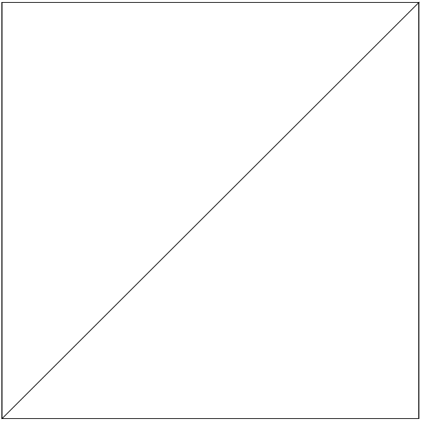
We consider the domain and introduce a hierarchy of meshes generated by uniform red refinement of the initial mesh shown in Figure 6.1 (left). For simplicity, we denote the meshes in the hierarchy by , where the subscript refers to the side length of the squares formed by joining opposing triangles. The coefficient is chosen to be piecewise constant with respect to the mesh with element values obtained as realizations of independent random variables uniformly distributed in the interval . Note that is assumed to be a negative power of two. For elements whose midpoints have a distance less than from a parabola, the corresponding element values are set to 10; see Figure 6.1 (right). The coefficient is set to zero for simplicity.
Note that all numerical experiments presented below can be reproduced using the code available at https://github.com/moimmahauck/Stokes_LOD_CR.

Exponential decay of basis functions
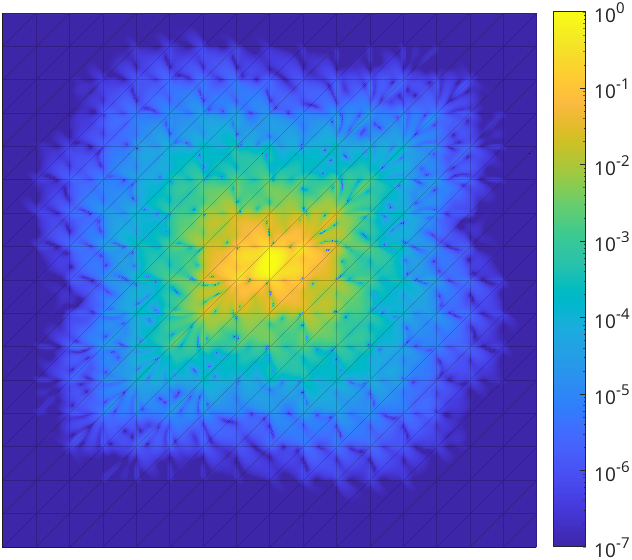
For the first numerical experiment we use the coefficient as described above for the value . The mesh for the fine-scale discretization is chosen to be , which sufficiently resolves the coefficient. This relatively large fine mesh size is necessary to compute the prototypical LOD basis functions needed to evaluate the localization errors.
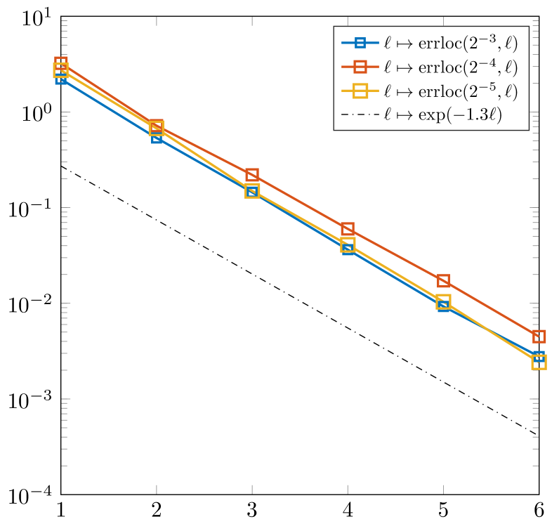
In Figure 6.2 (left), we illustrate the modulus of an exemplary basis function using a logarithmic color scale. A trained eye observes an exponential decay of the modulus with respect to the underlying coarse mesh, which we indicated in light gray. This supports the exponential decay result of Theorem 4.1. Next, we numerically investigate the localization error when replacing a prototypical basis function by its localized counterpart. For a given coarse mesh size and localization parameter , we define the -localization error as
In Figure 6.2 (right), one clearly observes an exponential decay of the -norm localization error as the localization parameter is increased. This supports the exponential approximation result from Theorem 4.2.
Optimal order convergence
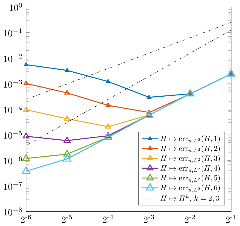
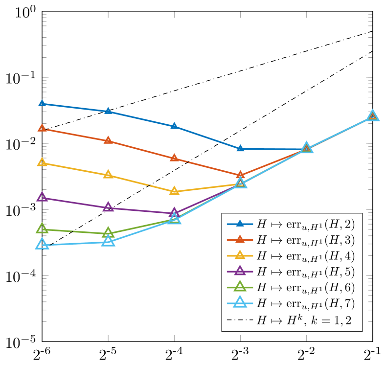
For the second numerical experiment, we use the coefficient from above for the value and choose the mesh for the fine-scale discretization. Furthermore, as right-hand side we use the function
In the following, we investigate the errors
where we recall that above denotes the reference solution computed on the fine mesh. For the - and -errors of the velocity approximation, we observe in Figure 6.3 the (almost) third and second order convergence, respectively, provided that the localization parameter is chosen sufficiently large. Recalling that , this is in line with the prediction from Theorem 5.1. For a fixed oversampling parameter, we observe that after a certain error level is reached, the error increases again as the mesh size is decreased. This is a well-known effect that occurs for some LOD methods such as [33, 30]. It can be overcome with a more sophisticated localization strategy; see, e.g., [21, 22, 12]. Such an improved localization strategy will be investigated in future work.
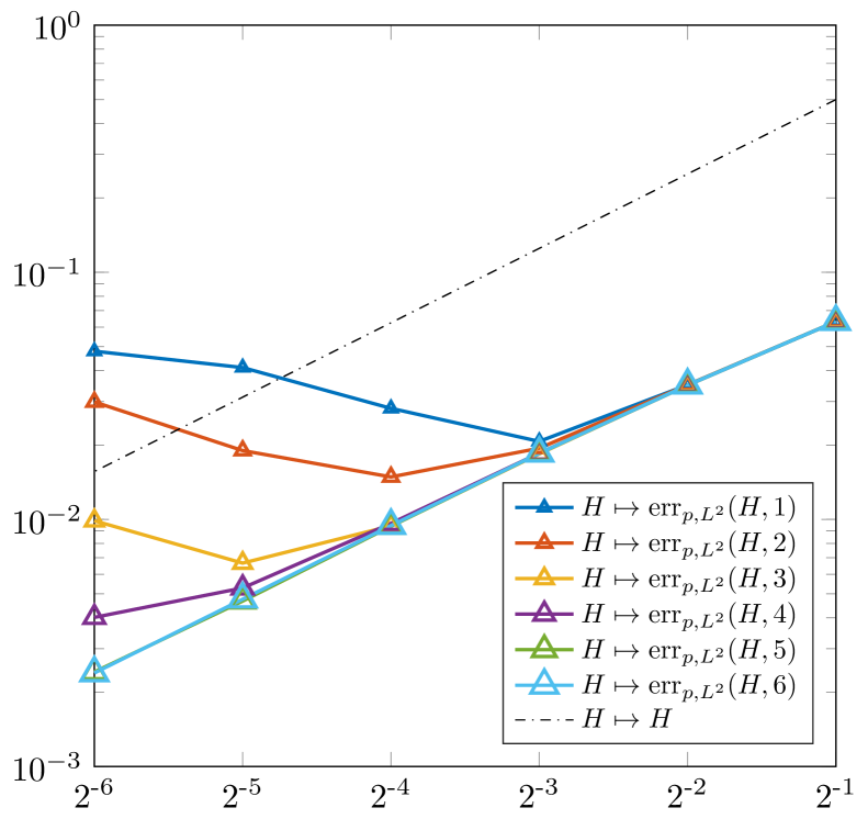
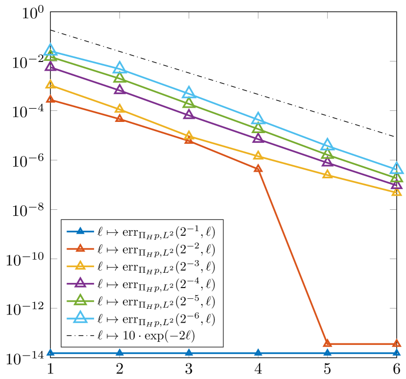
Now we turn to the pressure approximation. For the -error of the post-processed pressure approximation we observe in Figure 6.4 (left) the first-order convergence, again provided that the localization parameter is chosen sufficiently large. This observation is in line with Theorem 5.1. For the piecewise constant pressure approximation , we observe the exponential -convergence towards in Figure 6.4 (right), which is also consistent with Theorem 5.1. Note that the outliers are due to combinations of and where all patches are global, which implies that the pressure approximation coincides with , cf. Theorem 3.2.
Acknowledgment
The authors would like to thank Axel Målqvist for helpful discussions on the construction and analysis of the proposed method.
Appendix A Collection of frequently used bounds
Lemma A.1 (Local Poincaré-type inequality).
There exists independent of such that, for all and all satisfying for at least one face with , it holds that
| (A.1) |
Proof.
Lemma A.2 (Trace inequality).
There exists a constant independent of such that, for all and , it holds for any face with that
Proof.
The proof of this result can be done as in [13, Lem. 1.49], invoking the quasi-uniformity we assumed for the sequence of meshes considered. ∎
References
- ABF [99] P. Angot, C.-H. Bruneau, and P. Fabrie. A penalization method to take into account obstacles in incompressible viscous flows. Numer. Math., 81(4):497–520, 1999.
- AHP [21] R. Altmann, P. Henning, and D. Peterseim. Numerical homogenization beyond scale separation. Acta Numer., 30:1–86, 2021.
- AMS [24] C. Alber, C. Ma, and R. Scheichl. A mixed multiscale spectral generalized finite element method. ArXiv e-print 2403.16714, 2024.
- Bal [24] L. Balazi. Multi-scale Finite Element Method for incompressible flows in heterogeneous media: Implementation and Convergence analysis. PhD thesis, Institut polytechnique de Paris, 2024.
- BBF [13] D. Boffi, F. Brezzi, and M. Fortin. Mixed Finite Element Methods and Applications, volume 44 of Springer Series in Computational Mathematics. Springer, Heidelberg, 2013.
- BCDG [16] C. Bernardi, M. Costabel, M. Dauge, and V. Girault. Continuity properties of the inf-sup constant for the divergence. SIAM J. Math. Anal., 48(2):1250–1271, 2016.
- BEH [13] D. L. Brown, Y. Efendiev, and V. Hoang. An efficient hierarchical multiscale finite element method for Stokes equations in slowly varying media. Multiscale Model. Simul., 11(1):30–58, 2013.
- BEL+ [13] D. L. Brown, Y. Efendiev, G. Li, P. Popov, and V. Savatorova. Multiscale modeling of high contrast brinkman equations with applications to deformable porous media. In Poromechanics V, volume 7, page 1991–1996. American Society of Civil Engineers, 2013.
- BL [11] I. Babuška and R. Lipton. Optimal local approximation spaces for generalized finite element methods with application to multiscale problems. Multiscale Model. Simul., 9(1):373–406, 2011.
- CEL [18] E. T. Chung, Y. Efendiev, and W. T. Leung. Constraint energy minimizing generalized multiscale finite element method. Comput. Methods Appl. Mech. Engrg., 339:298–319, 2018.
- CR [73] M. Crouzeix and P.-A. Raviart. Conforming and nonconforming finite element methods for solving the stationary Stokes equations I. Recherche Opérationnelle, 7(R3):33–75, 1973.
- DHM [23] Z. Dong, M. Hauck, and R. Maier. An improved high-order method for elliptic multiscale problems. SIAM J. Numer. Anal., 61(4):1918–1937, 2023.
- DPE [12] D. A. Di Pietro and A. Ern. Mathematical Aspects of Discontinuous Galerkin Methods. Springer, 2012.
- EE [03] W. E and B. Engquist. The heterogeneous multiscale methods. Commun. Math. Sci., 1(1):87–132, 2003.
- EG [04] A. Ern and J.-L. Guermond. Theory and Practice of Finite Elements, volume 159 of Applied Mathematical Sciences. Springer New York, 2004.
- EGH [13] Y. Efendiev, J. Galvis, and T. Y. Hou. Generalized multiscale finite element methods (GMsFEM). J. Comput. Phys., 251:116–135, 2013.
- FAO [22] Q. Feng, G. Allaire, and P. Omnes. Enriched nonconforming multiscale finite element method for Stokes flows in heterogeneous media based on high-order weighting functions. Multiscale Model. Simul., 20(1):462–492, 2022.
- Gal [14] D. Gallistl. Adaptive finite element computation of eigenvalues. PhD thesis, Humboldt-Universität zu Berlin, Mathematisch-Naturwissenschaftliche Fakultät II, 2014.
- GGS [12] L. Grasedyck, I. Greff, and S. Sauter. The AL basis for the solution of elliptic problems in heterogeneous media. Multiscale Model. Simul., 10(1):245–258, 2012.
- GP [10] F. Gutiérrez and M. A. Parada. Numerical modeling of time-dependent fluid dynamics and differentiation of a shallow basaltic magma chamber. J. Petrol., 51(3):731–762, 2010.
- HP [13] P. Henning and D. Peterseim. Oversampling for the multiscale finite element method. Multiscale Model. Simul., 11(4):1149–1175, 2013.
- [22] M. Hauck and D. Peterseim. Multi-resolution localized orthogonal decomposition for Helmholtz problems. Multiscale Model. Simul., 20(2):657–684, 2022.
- [23] M. Hauck and D. Peterseim. Super-localization of elliptic multiscale problems. Math. Comp., 92(341):981–1003, 2022.
- HW [97] T. Y. Hou and X.-H. Wu. A multiscale finite element method for elliptic problems in composite materials and porous media. J. Comput. Phys., 134(1):169–189, 1997.
- JL [24] G. Jankowiak and A. Lozinski. Non-conforming multiscale finite element method for Stokes flows in heterogeneous media. Part II: error estimates for periodic microstructure. Discrete Continuous Dyn. Syst. Ser. B., 29(5):2298–2332, 2024.
- JLM+ [17] V. John, A. Linke, C. Merdon, M. Neilan, and L. G. Rebholz. On the divergence constraint in mixed finite element methods for incompressible flows. SIAM Rev., 59(3):492–544, 2017.
- Lad [63] O.A. Ladyzhenskaia. The Mathematical Theory of Viscous Incompressible Flow. Mathematical Theory of Viscous Incompressible Flow. Gordon and Breach, 1963.
- LBLL [14] C. Le Bris, F. Legoll, and A. Lozinski. MsFEM à la Crouzeix-Raviart for highly oscillatory elliptic problems. In Partial Differential Equations: Theory, Control and Approximation: In Honor of the Scientific Heritage of Jacques-Louis Lions, pages 265–294. Springer Berlin Heidelberg, 2014.
- LM [09] M. G. Larson and A. Målqvist. A mixed adaptive variational multiscale method with applications in oil reservoir simulation. Math. Models Methods Appl. Sci., 19(07):1017–1042, 2009.
- Mai [21] R. Maier. A high-order approach to elliptic multiscale problems with general unstructured coefficients. SIAM J. Numer. Anal., 59(2):1067–1089, 2021.
- MHH [16] A. Målqvist, P. Henning, and F. Hellman. Multiscale mixed finite elements. Discrete Contin. Dyn. Syst. - S., 9(5):1269–1298, 2016.
- MNLD [15] B. P. Muljadi, J. Narski, A. Lozinski, and P. Degond. Nonconforming multiscale finite element method for Stokes flows in heterogeneous media. Part I: methodologies and numerical experiments. Multiscale Model. Simul., 13(4):1146–1172, 2015.
- MP [14] A. Målqvist and D. Peterseim. Localization of elliptic multiscale problems. Math. Comp., 83(290):2583–2603, 2014.
- MP [20] A. Målqvist and D. Peterseim. Numerical homogenization by localized orthogonal decomposition, volume 5 of SIAM Spotlights. Society for Industrial and Applied Mathematics (SIAM), Philadelphia, PA, 2020.
- MS [02] A.-M. Matache and C. Schwab. Two-scale FEM for homogenization problems. ESAIM: Math. Model. Numer. Anal., 36(4):537–572, 2002.
- MSD [22] C. Ma, R. Scheichl, and T. Dodwell. Novel design and analysis of generalized finite element methods based on locally optimal spectral approximations. SIAM J. Numer. Anal., 60(1):244–273, 2022.
- Owh [17] H. Owhadi. Multigrid with rough coefficients and multiresolution operator decomposition from hierarchical information games. SIAM Rev., 59(1):99–149, 2017.
- PW [60] L. E. Payne and H. F. Weinberger. An optimal Poincaré inequality for convex domains. Arch. Rational Mech. Anal., 5:286–292 (1960), 1960.
- VZ [19] R. Verfürth and P. Zanotti. A quasi-optimal Crouzeix–Raviart discretization of the Stokes equations. SIAM J. Numer. Anal., 57(3):1082–1099, 2019.