GARCH option valuation with long-run and short-run volatility components: A novel framework ensuring positive variance

Abstract

Christoffersen, Jacobs, Ornthanalai, and Wang (2008) (CJOW) proposed an improved Generalized Autoregressive Conditional Heteroskedasticity (GARCH) model for valuing European options, where the return volatility is comprised of two distinct components. Empirical studies indicate that the model developed by CJOW outperforms widely-used single-component GARCH models and provides a superior fit to options data than models that combine conditional heteroskedasticity with Poisson-normal jumps. However, a significant limitation of this model is that it allows the variance process to become negative. Oh and Park (2023) partially addressed this issue by developing a related model, yet the positivity of the volatility components is not guaranteed, both theoretically and empirically. In this paper we introduce a new GARCH model that improves upon the models by CJOW and Oh and Park (2023), ensuring the positivity of the return volatility. In comparison to the two earlier GARCH approaches, our novel methodology shows comparable in-sample performance on returns data and superior performance on S&P500 options data.

Keywords Volatility term structure; GARCH; Option pricing; Component model; Positive volatility.

1 Introduction

Building on the pioneering work of Engle and Lee (1999), Christoffersen, Jacobs, Ornthanalai, and Wang (2008) (CJOW) proposed an interesting GARCH model with two volatility components, hereafter referred to as the GARCH-CJOW model. One volatility component is a long-run component that can be modeled as a mean-reverting or as a fully persistent process, while the other is a short-run mean-reverting component with zero mean. As shown by the authors, the model allows for an efficient valuation of European options and its most distinctive feature is its ability to accurately describe the implied volatility term structure. In particular, the empirical analysis that CJOW conducted on both long-maturity and short-maturity options demonstrates superior pricing performance compared to the popular GARCH model with a single volatility component developed by Heston and Nandi (2000) and a GARCH(1,1) model augmented with Poisson-normal jumps. Owing to its well-documented empirical performance, the GARCH-CJOW model has gained popularity in the GARCH literature and has been used for pricing S&P500 options in Corsi et al. (2013) and VIX futures in Cheng et al. (2023).

Despite its success, Bormetti et al. (2015) and Oh and Park (2023) provide evidence that the GARCH-CJOW model fails to guarantee positive volatilities for parameter sets commonly encountered in financial practice. This raises significant modeling concerns for out-of-sample (volatility) analysis and for option pricing, especially for medium to long-maturing options. Even though Bormetti et al. (2015) state that the likelihood of obtaining negative volatilities is extremely low, Oh and Park (2023) further analyze the performances of the GARCH-CJOW model and find that it can generate a consistent number of negative volatility trajectories. Then, to address the issue, they propose an enhancement of the GARCH-CJOW model, hereafter referred to as GARCH-OP, which allows for the pricing of SPX options and VIX derivatives. However, this model also does not ensure positivite volatility.

In this paper, we investigate further the issue of negative volatility of the GARCH-CJOW model and its implications for option pricing. Contrary to the conclusions drawn by Bormetti et al. (2015), we demonstrate that, for parameter sets established in the empirical literature, the GARCH-CJOW model generates a consistent number of negative volatility trajectories. Additionally, the GARCH-OP model also produces negative volatilities, a concern that becomes more pronounced for longer time horizons. We also find that this issue affects the computation of option prices, as it is based on an inversion formula where the integrands for longer maturities may diverge.

To fix these issues, we propose an improvement to the model developed by CJOW that ensures the positivity of the volatility process by properly specifying the impact of the innovation on volatility. This new model, which allows for a well-posed option semi-closed form valuation, will be referred to as corrected positive component GARCH model, or, in short, GARCH-CPC. In contrast to the GARCH-CJOW model, the semi-closed formula of the GARCH-CPC model can be safely used in every option pricing scenario, even for large option maturities.

Moreover, we compare the performance of the GARCH-CJOW, GARCH-CPC and GARCH-OP models in the valuation of a large panel of options written on the S&P500 index. We find that the novel GARCH-CPC model offers a feasible and efficient solution for computing option prices using affine formulas with greater accuracy than both the GARCH-CJOW and the GARCH-OP models.

The remainder of this paper is structured as follows. In Section 2, we briefly recall the GARCH-CJOW and the GARCH-OP models, showing the negativity issues affecting these approaches and their implications for option pricing. Section 3 proposes the GARCH-CPC model. After deriving the risk-neutral dynamics, we provide the formulas for option valuation. Section 4 presents an empirical study conducted on returns and option data. Finally, Section 5 concludes.

2 Return dynamics with volatility components

The volatility component model proposed by CJOW for the return process $R_{t}=\ln{\left(\frac{S_{t}}{S_{t-1}}\right)}$, where $S_{t}$ denotes the spot price, is given by the following equations (under the physical measure):

$$R_{t+1} =r+\lambda h_{t+1}+\sqrt{h_{t+1}}Z_{t+1},$$ (1)

$$h_{t+1} =q_{t+1}+\tilde{\beta}(h_{t}-q_{t})+\alpha\left(Z^{2}_{t}-1-2\gamma_{1}\sqrt{h_{t}}Z_{t}\right),$$ (2)

$$q_{t+1} =\omega+\rho q_{t}+\varphi\left(Z^{2}_{t}-1-2\gamma_{2}\sqrt{h_{t}}Z_{t}\right),$$ (3)

where $r$ denotes the risk-free rate, $Z_{t}\overset{iid}{\sim}N(0,1)$. CJOW refer to $q_{t}$ and $h_{t}-q_{t}$ as the long-run and the short-run variance component, respectively. They impose the parameter constraints $\omega\geq 0$, $\alpha>0$, $\varphi>0$, $\tilde{\beta}<1$ and $\rho<1$. In the long-run we have that $\mathbb{E}[h_{t}]=\mathbb{E}[q_{t}]={\omega}/(1-\rho)$.

As pointed out in Bormetti et al. (2015) and Oh and Park (2023), the model (1)-(3) does not guarantee that the total variance $h_{t}$ remains positive. Therefore, in Oh and Park (2023), the following model, hereafter referred to as GARCH-OP, has been proposed as a more robust alternative to address the negative volatility issue that affects the GARCH-CJOW model:

$$R_{t+1} =r+\lambda h_{t+1}+\sqrt{h_{t+1}}Z_{t+1},$$ (4)

$$h_{t+1} =q_{t+1}+\tilde{\beta}(h_{t}-q_{t})+\alpha\left(Z_{t}-\gamma_{1}\sqrt{h_{t}}\right)^{2}-\omega-\alpha\gamma^{2}_{1}h_{t},$$ (5)

$$q_{t+1} =\omega+\rho q_{t}+\varphi\left(Z_{t}-\gamma_{2}\sqrt{h_{t}}\right)^{2},$$ (6)

where the long-term means are given by $\begin{pmatrix}\mathbb{E}[h_{t}]&\mathbb{E}[q_{t}]\end{pmatrix}^{\top}=(I_{2}-P)^{-1}R$, where $I_{2}$ denote a $2\times 2$ identity matrix, $P=\begin{pmatrix}\tilde{\beta}+\varphi\gamma^{2}_{2}&\rho-\tilde{\beta}\\ \varphi\gamma^{2}_{2}&\rho\end{pmatrix}$ and $R=\begin{pmatrix}\alpha+\varphi\\ \omega+\varphi\end{pmatrix}$.

2.1 Model issues

In this section, we will document the issues of model (1)-(3) and model (4)-(6) related to the negative values that the variance can take through a few test cases. Using parameters established in the empirical literature, we will show via statistical simulation how many variance trajectories $h_{t}$ can turn negative, and we will examine the implications for option pricing.

2.1.1 Negative volatility trajectories

For the model (1)-(3) we initially consider two sets of parameters available in the literature, namely, those in Christoffersen et al. (2008) and in Cheng et al. (2023), which we denote as CJOW08 and CCLT23, respectively. These parameters are reported in Table 1. We note that equation (1) in Cheng et al. (2023) specifies $\lambda-\frac{1}{2}$ instead of just $\lambda$ as in equation (1) in the present paper, so in Table 1 we adjusted the value of $\lambda$ accordingly. Whereas, for model in (4)-(6) we consider the same parameters as in Oh and Park (2023), which we denote OP23 and we report in Table 1.

Table 1: Model parameters.

Parameter	$\omega$	$\alpha$	$\gamma_{1}$	$\tilde{\beta}$	$\varphi$	$\gamma_{2}$	$\rho$	$\lambda$
CJOW08	8.208e-07	1.580e-06	415.100	0.6437	2.480e-06	63.240	0.9896	2.092
CCLT23	7.776e-07	1.380e-06	402.352	0.862	1.795e-06	73.205	0.991	1.357
OP23	-1.57e-06	0.190e-06	7050	0.922	2.62e-06	89	0.983	-7.88

We perform a Monte Carlo exercise where we simulate the trajectories of the variance in equations (2) and (5) to check if, and how many of them, turn negative. The simulation consists in generating 1,000,000 paths of innovations ${Z_{t}}$ from $t=0$ to a given time horizon $T>0$. Using equations (2)-(3) and (5)-(6), for each path we compute the variance $h_{t}$ and count the number of trajectories such that $h_{t}$ becomes negative for some $t\leq T$. We set $S_{0}=100$, $r=10^{-5}$ and, following Oh and Park (2023), we choose $q_{0}$ and $h_{0}$ such that the (annualized) initial volatility states $\sqrt{252q_{0}}$ and $\sqrt{252h_{0}}$ are equal to $5\%$ and $10\%$, respectively. The results, illustrated in Table 2, show that as $T$ increases, the number of negative trajectories also increases for both the GARCH-CJOW and GARCH-OP models. However, as documented in Oh and Park (2023), the number of negative trajectories generated by the GARCH-OP model is significantly lower compared to the GARCH-CJOW model.

Table 2: Negative trajectories for the variance $h_{t}$ out of 1,000,000 simulations for time horizon $T$.

	Initial volatility $\left(\sqrt{252q_{0}},\sqrt{252h_{0}}\right)$
	(5% , 5%)			(10% , 10%)
	GARCH-CJOW		GARCH-OP	GARCH-CJOW		GARCH-OP
$T$	CJOW08	CCLT23	OP23	CJOW08	CCLT23	OP23
15	226,386	185,403	2,328	0	0	0
30	287,888	235,937	7,848	317	0	0
50	315,161	251,841	10,422	3,671	115	7
80	330,745	258,352	11,023	10,034	481	33
120	339,795	260,234	11,112	16,883	891	41
252	351,374	261,183	11,114	29,129	1,465	44

2.1.2 Option pricing

In this subsection, after briefly recalling formulas commonly used to compute option prices, we empirically analyze the consequences of generating negative volatility trajectories for option valuation in the GARCH-CJOW and GARCH-OP models.

As shown by Heston and Nandi (2000) and further utilized by CJOW, the inversion formula developed in Gil-Pelaez (1951) yields the following expression for a European call option on a non-dividend paying stock with spot price $S_{t}$, strike price $K$ and expiration date $T$:

$$C_{t}=\frac{1}{2}S_{t} +\frac{e^{-r(T-t)}}{\pi}\int_{0}^{\infty}\text{Re}\left[\frac{K^{-i\phi}f^{*}(t,T;i\phi+1)}{i\phi}\right]d\phi$$ (7)

$$-Ke^{-r(T-t)}\left(\frac{1}{2}+\frac{1}{\pi}\int_{0}^{\infty}\text{Re}\left[\frac{K^{-i\phi}f^{*}(t,T;i\phi)}{i\phi}\right]d\phi\right),$$

where $\text{Re}[\cdot]$ denotes the real part of a complex number and $f^{*}(t,T;i\phi)$ represents the conditional characteristic function of the terminal log-stock price under the risk-neutral measure. The risk-neutral conditional characteristic function of the GARCH-CJOW and GARCH-OP models can be computed as follows:

$$f^{*}(t,T;\phi)=S_{t}^{\phi}\exp{\{A_{t}(\phi)+B_{1,t}(\phi)(h_{t+1}-q_{t+1})+B_{2,t}(\phi)q_{t+1}\}},\quad t<T,$$ (8)

where the expressions of $A_{t}(\phi)$, $B_{1,t}(\phi)$ and $B_{2,t}(\phi)$ can be obtained using equations (25) in the paper by Christoffersen et al. (2008) for the GARCH-CJOW model and using equations (8) in the paper by Oh and Park (2023) for the GARCH-OP model.

Let us now focus on the integrand functions in (7):

$$I_{1}=\text{Re}\left[\frac{K^{-i\phi}f^{*}(t,T;i\phi+1)}{i\phi}\right],\quad I_{2}=\text{Re}\left[\frac{K^{-i\phi}f^{*}(t,T;i\phi)}{i\phi}\right].$$ (9)

For both the GARCH-CJOW and GARCH-OP models, we check the integrability of $I_{1}$ and $I_{2}$, by analyzing the behavior of $I_{1}$ and $I_{2}$ as functions of $\phi$ and for different option maturities $T=15,30,50,80,120,252$. For comparison purposes, we also consider the values of $I_{1}$ and $I_{2}$ for the popular GARCH model developed in Heston and Nandi (2000), hereafter GARCH-HN:

$$R_{t+1} =r+\lambda h_{t+1}+\sqrt{h_{t+1}}Z_{t+1},$$ (10)

$$h_{t+1} =\omega+\tilde{\beta}h_{t}+\alpha\left(Z_{t}-\gamma_{1}\sqrt{h_{t}}\right)^{2}.$$ (11)

Similarly to the GARCH-CJOW model, for the GARCH-HN model we use parameters obtained by Christoffersen et al. (2008) and Cheng et al. (2023), which are reported in Table 3. We note that, for the GARCH-HN model, option prices can be computed using equation (7) in conjunction with the risk-neutral conditional characteristic function obtained by Heston and Nandi (2000).

Table 3: Parameters of the GARCH-HN obtained by CJOW and Cheng et al. (2023).

Parameter	$\omega$	$\alpha$	$\gamma_{1}$	$\tilde{\beta}$	$\lambda$
CJOW08	2.101e-17	3.317e-06	1.276e+02	0.9552	2.231
CCLT23	1.744e-06	3.098e-06	120.967	0.935	1.395

Figures 1-5 show the behavior of $|I_{1}|$ and $|I_{2}|$ for the GARCH-HN, GARCH-CJOW and GARCH-OP models. In particular, Figures 1 and 2 display the behavior of $|I_{1}|$ and $|I_{2}|$, respectively, for the GARCH-HN model using the parameters CJOW08 and CCLT23 in Table 1. As the initial (annualized) volatility state we set $\sqrt{252h_{0}}$ equal to either $5\%$ or $10\%$ and we set $r=10^{-5}$ and $S_{0}=K=100$. Instead, for the GARCH-CJOW model we show the behavior of $|I_{1}|$ and $|I_{2}|$ in Figures 3 and 4 and for the GARCH-OP model in Figure 5. As for the initial volatility states, again we set $\sqrt{252h_{0}}$ and $\sqrt{252q_{0}}$ equal to $5\%$ and $10\%$, and we set $r=10^{-5}$ and $S_{0}=K=100$.

As we may notice, for both the CJOW08 and CCLT23 parameters, the GARCH-HN model does not show any integrability issue for $I_{1}$ and $I_{2}$ in equation (9), whereas Figures 3, 4 and 5 clearly show that $I_{1}$ and $I_{2}$ explode for almost all the considered maturities. Only for $T=15$ and for the $10\%$ initial volatility state both the GARCH-CJOW and GARCH-OP models do not exhibit any issues.

Figure 1: Behavior of $I_{1}$ (left) and $I_{2}$ (right), as functions of $\phi$ for different values of $T$ for the GARCH-HN model. We set $S_{0}=K=100$, $r=10^{-5}$ and $\sqrt{252h_{0}}=5\%$. We use the CJOW08 parameters (top panels) and the CCLT23 parameters as in Table 1 (bottom panels).

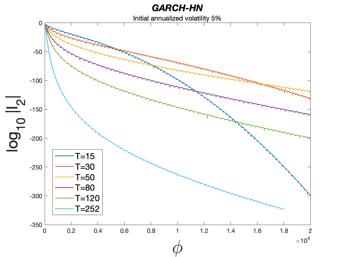
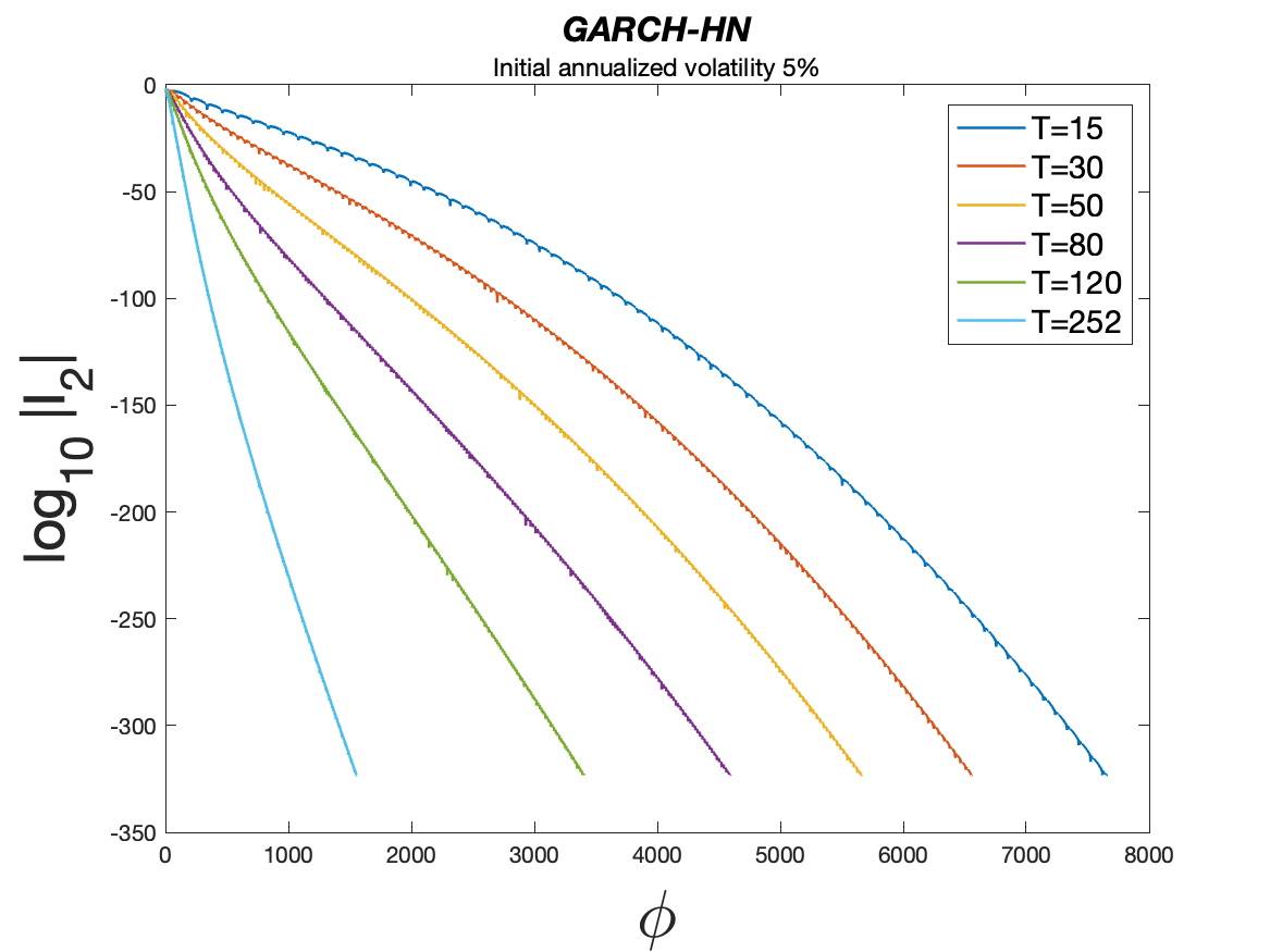
Figure 2: Behavior of $I_{1}$ (left) and $I_{2}$ (right), as functions of $\phi$ for different values of $T$ for the GARCH-HN model. We set $S_{0}=K=100$, $r=10^{-5}$ and $\sqrt{252h_{0}}=10\%$. We use the CJOW08 parameters (top panels) and the CCLT23 parameters as in Table 1 (bottom panels).

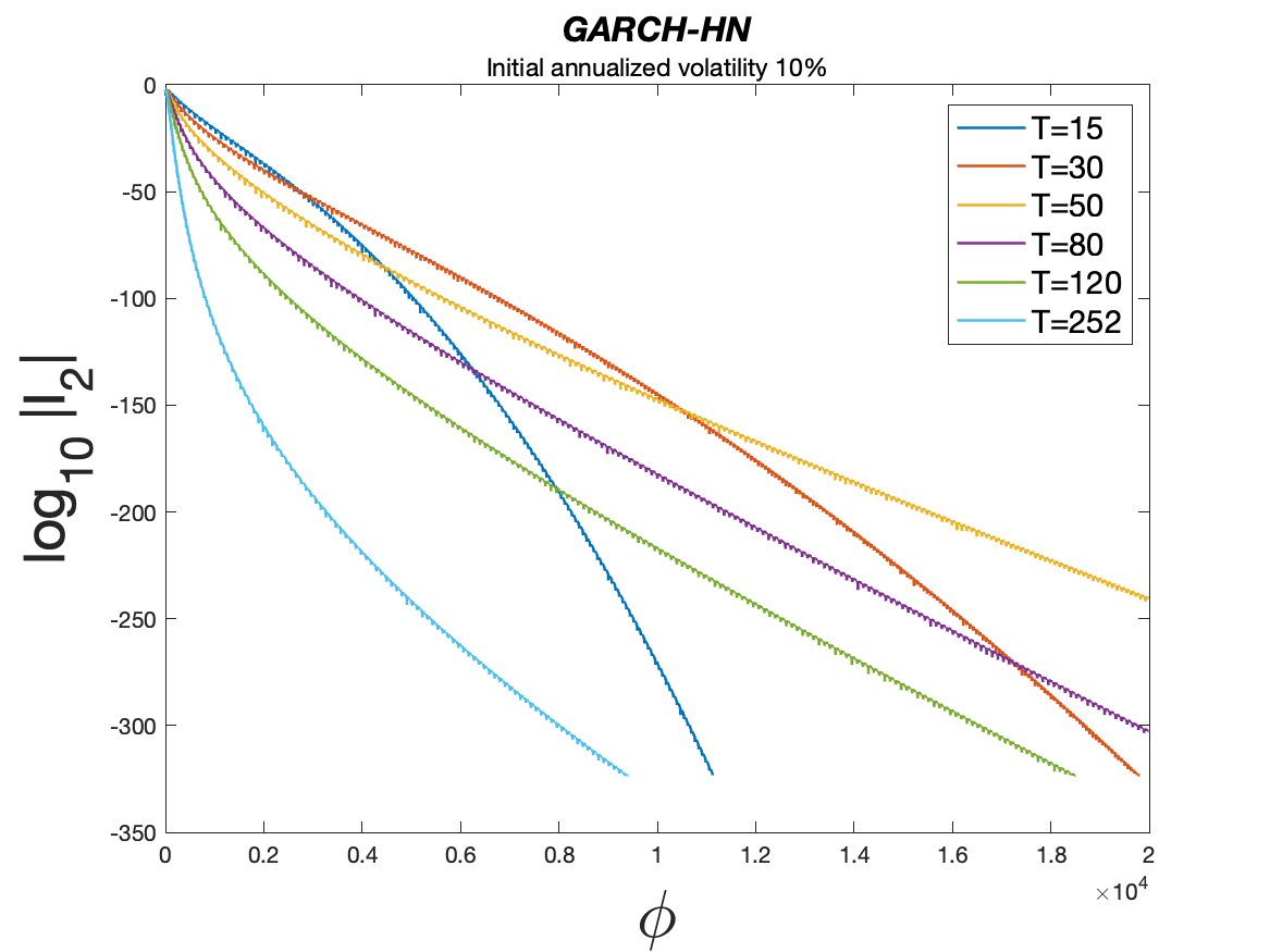
Figure 3: Behavior of $I_{1}$ (left) and $I_{2}$ (right), as functions of $\phi$ for different values of $T$ for the GARCH-CJOW model. We used $S_{0}=K=100$, $r=10^{-5}$ and the initial volatility states $\sqrt{252h_{0}}=5\%$ and $\sqrt{252q_{0}}=5\%$. We use the CJOW08 parameters (top panels) and the CCLT23 parameters as in Table 1 (bottom panels).

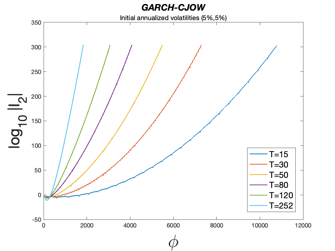
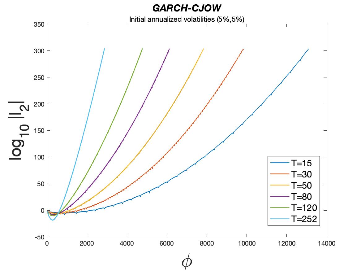
Figure 4: Behavior of $I_{1}$ (left) and $I_{2}$ (right), as functions of $\phi$ for different values of $T$ for the GARCH-CJOW model. We used $S_{0}=K=100$, $r=10^{-5}$ and the initial volatility states $\sqrt{252h_{0}}=10\%$ and $\sqrt{252q_{0}}=10\%$. We use the CJOW08 parameters (top panels) and the CCLT23 parameters as in Table 1 (bottom panels).

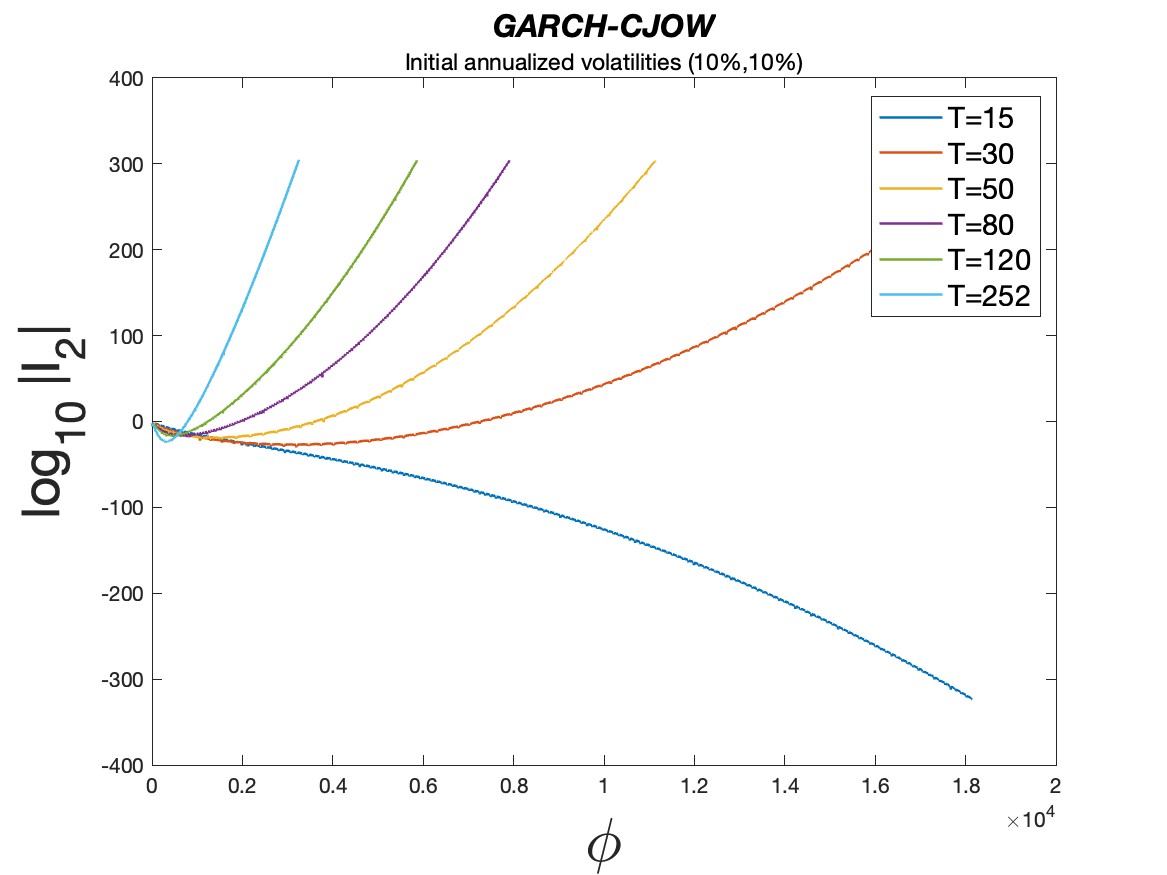
Figure 5: Behavior of $I_{1}$ (left) and $I_{2}$ (right), as functions of $\phi$ for different values of $T$ for the GARCH-OP model with the parameters OP23 of Table 1. We set $S_{0}=K=100$, $r=10^{-5}$. We use $\sqrt{252h_{0}}=\sqrt{252q_{0}}=5\%$ (top panels) and $\sqrt{252h_{0}}=\sqrt{252q_{0}}=10\%$ (bottom panels).

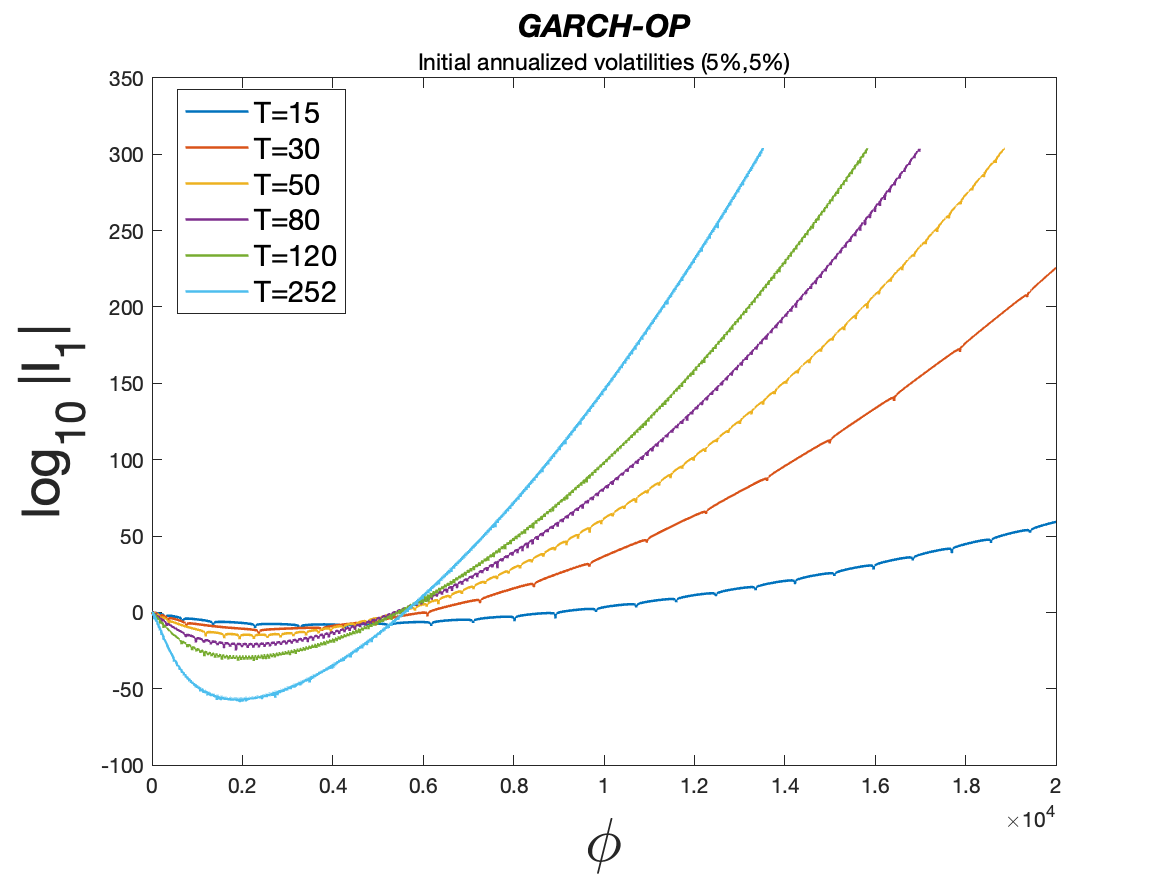
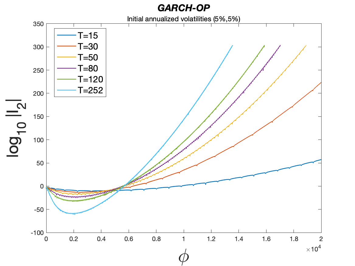
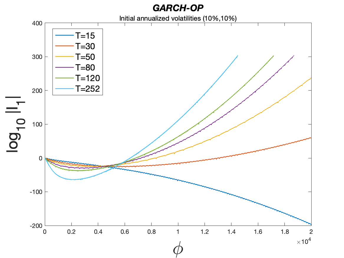
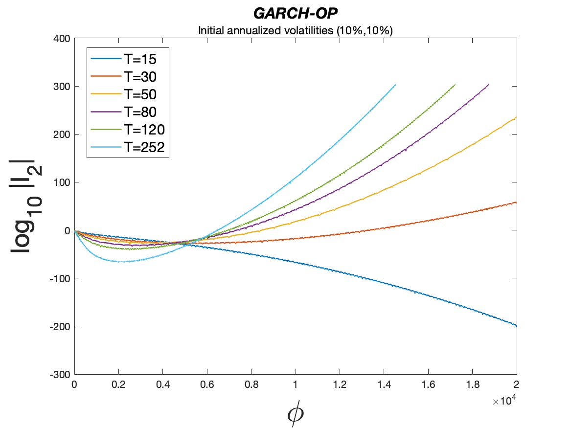
3 An improved two-component GARCH model for option valuation

In this section, we propose a component volatility model that enhances the one developed by CJOW by ensuring that the volatility remains positive. We name this model GARCH-CPC, which stands for Corrected Positive Component GARCH. The model consists of the following equations:

$$R_{t+1} =r+\lambda h_{t+1}+\sqrt{h_{t+1}}Z_{t+1},$$ (12)

$$h_{t+1} =q_{t+1}+\tilde{\beta}(h_{t}-q_{t})+\alpha\left\{\left(Z_{t}-\gamma_{1}\sqrt{h_{t}}\right)^{2}-\gamma^{2}_{1}q_{t}\right\},$$ (13)

$$q_{t+1} =\omega+\rho q_{t}+\varphi\left(Z_{t}-\gamma_{2}\sqrt{h_{t}}\right)^{2},$$ (14)

where $Z_{t}\overset{iid}{\sim}N(0,1)$ and $q_{t}$ represents a process related to the long-run volatility component as in the GARCH-CJOW model. To ensure the positivity of $h_{t}$, we assume the following conditions for the parameters: $\omega\geq 0$, $\alpha>0$, $\varphi>0$ and $\tilde{\beta}+\alpha\gamma^{2}_{1}<\rho<1$. Substituting equation (14) into (13) immediately shows that these parameter conditions are sufficient to guarantee the positivity of $h_{t}$ for all $t$. The long-run means are given by $\begin{pmatrix}\mathbb{E}[h_{t}]&\mathbb{E}[q_{t}]\end{pmatrix}^{\top}=(I_{2}-P)^{-1}R$, where $I_{2}$ denote a $2\times 2$ identity matrix, $R=\begin{pmatrix}\omega+\alpha+\varphi\\ \omega+\varphi\end{pmatrix}$ and $P=\begin{pmatrix}\tilde{\beta}+\alpha\gamma^{2}_{1}+\varphi\gamma^{2}_{2}&\rho-\tilde{\beta}-\alpha\gamma^{2}_{1}\\ \varphi\gamma^{2}_{2}&\rho\end{pmatrix}$.

We note that, for the model in equations (2)-(3), $\mathbb{E}[h_{t}-q_{t}]=0$. In contrast, for equations (5)-(6) it holds that $\mathbb{E}[h_{t}-q_{t}]={\alpha}/(1-\tilde{\beta})$ and for equations (13)-(14) we have $\mathbb{E}[h_{t}-q_{t}]={\alpha}/(1-\tilde{\beta}-\alpha\gamma^{2}_{1})$. Therefore, unlike in the GARCH-CJOW model, the long-run volatility component in the GARCH-OP and GARCH-CPC models is represented not by $q_{t}$, but rather by $q_{t}+\bar{h}$, where $\bar{h}=\frac{\alpha}{1-\tilde{\beta}}$ for the GARCH-OP model, and $\bar{h}=\frac{\alpha}{1-\tilde{\beta}-\alpha\gamma^{2}_{1}}$ for the GARCH-CPC model.

3.1 The risk-neutral GARCH-CPC dynamics

Following Christoffersen et al. (2008), we risk-neutralize the dynamics for the GARCH-CPC model as follows:

$$R_{t+1} =r-\frac{1}{2}h_{t+1}+\sqrt{h_{t+1}}Z^{*}_{t+1},$$ (15)

$$h_{t+1} =q_{t+1}+\tilde{\beta}(h_{t}-q_{t})+\alpha\left(Z^{*}_{t}-\gamma^{*}_{1}\sqrt{h_{t}}\right)^{2}-\alpha(\gamma^{*}_{1})^{2}q_{t},$$ (16)

$$q_{t+1} =\omega+\rho q_{t}+\varphi\left(Z^{*}_{t}-\gamma^{*}_{2}\sqrt{h_{t}}\right)^{2},$$ (17)

with $\gamma^{*}_{i}=\gamma_{i}+\frac{1}{2}+\lambda$ for $i=1,2$ and $Z^{*}_{t}\sim N(0,1)$.

3.2 Moment generating function

To perform option valuation, we derive the moment generating function associated to the terminal log-spot price of equation (15).

Proposition 1

The conditional moment generating function for the logarithm of the terminal log-price $\ln S_{T}$, denoted by $f(t,T;\phi)$, can be computed as

$$f(t,T;\phi)=e^{\phi\log S_{t}+A_{t}(\phi)+B_{1,t}(\phi)(h_{t+1}-q_{t+1})+B_{2,t}(\phi)q_{t+1}},\quad t<T,$$ (18)

where the expressions for $A_{t}(\phi)$, $B_{1,t}(\phi)$ and $B_{2,t}(\phi)$ are derived in equation (24) in the Appendix.

4 Empirical results for returns and options

In this section, we examine the goodness-of-fit of the GARCH-CJOW, GARCH-OP and the GARCH-CPC models on both returns and options data.

The data for the daily levels of Adjusted Close Price for the S&P500 returns series is retrieved from Refinitiv Datastream. As a proxy of the risk-free interest rate, we utilize the 3-month Treasury Bill rate and we gathered its time series data from the Federal Funds Effective Rate (FRED) dataset. For the returns, we considered two different periods: one covering the same period considered by CJOW, from July 2, 1962, to December 31, 2001 (labeled as “Period 1") resulting in 9943 days, and another covering more recent data from January 2, 2002, to December 29, 2023 (labeled as “Period 2") for a total of 5537 days.

We consider both Put and Call European options written on the S&P500 index, with data retrieved from Thomson Reuters Eikon Datastream. The options we examined have maturities ranging from 2020 to 2023 and we consider the option daily prices from February 10, 2020, to December 29, 2023. As a common practice, following Christoffersen et al. (2012), Ballestra et al. (2023), and Ballestra et al. (2024), we apply several exclusion filters retaining a total of 14,247 options prices. In particular, we keep only the options with time-to-maturity between 14 and 365 days and we select only out-of-the-money Put and Call options (we compute the moneyness as $K/S_{t}$, where $K$ is the strike price and $S_{t}$ is the underlying index level), and we filter out illiquid quotes by selecting only the six most liquid strikes at each maturity, and we consider option quotes only on Wednesday. Finally, we remove price quotes lower than $3.8\$$.

Following CJOW, the estimation we conducted relies on maximum likelihood estimation using only the log-returns. The results for Period 1 and Period 2 are shown in Table 4. For Period 1, since we considered the same time frame as CJOW, we included the parameters they estimated in their article. To evaluate the goodness-of-fit on the returns data, we also include log-likelihood values alongside standard information criteria such as AIC and BIC. Finally, the fit to the option data is assessed using a standard metric, the implied volatility root mean square error:

$$\text{IVRMSE(\%)}=100\times\sqrt{\frac{1}{N}\sum_{i=1}^{N}\left(\textit{IV}^{MKT}_{i}-\textit{IV}^{MOD}_{i}\right)^{2}},$$ (19)

where $\textit{IV}^{MKT}_{i}$ and $\textit{IV}^{MOD}_{i}$ denote the market and the model implied volatilities of the $i$-th option price, respectively.

Generally speaking, for both periods, the GARCH-CPC and GARCH-OP models exhibit slightly worse fit on the returns data compared to the GARCH-CJOW, as indicated by AIC and BIC values. However, for the GARCH-CJOW model it was not possible to calculate all the option prices due to the issues of negative variance outlined previously in Section 2.1.2.

Thus, the fit to option data was assessable only for the GARCH-CPC and GARCH-OP models. In particular, the GARCH-CPC displayed IVRMSE values of 5.7% and 4.9% for Period 1 and Period 2, respectively. For the GARCH-CJOW model the “NaN" values, reported at the bottom of Table 4, indicate that it was not possible to compute prices for all the $N$ options based on the numerical integration of (7). Whereas, for the parameters estimated in Table 4, the GARCH-OP did not encounter any issues in pricing the options we considered but returned higher pricing errors compared to the GARCH-CPC model.

Table 4: Maximum likelihood estimation results

	Period 1			Period 2
	GARCH-CPC	GARCH-OP	GARCH-CJOW	GARCH-CPC	GARCH-OP	GARCH-CJOW
$\omega$	1.546e-16	8.678e-12	8.208e-07***	6.177e-14	6.689e-09	7.735e-07***
	(7.420e-09)	(1.911e-08)	(7.620e-08)	(3.860e-09)	(5.651e-09)	(1.957e-07)
$\alpha$	2.923e-06***	1.337e-06***	1.580e-06***	1.003e-06**	3.004e-06***	3.520e-06***
	(1.392e-06)	(1.339e-07)	(2.430e-07)	(5.463e-07)	(6.094e-07)	(1.234e-06)
$\gamma_{1}$	140.269***	438.588***	4.151e+02**	343.652***	337.450***	227.209***
	(29.868)	(73.865)	(6.341e+01)	(123.759)	(59.820)	(82.479)
$\tilde{\beta}$	0.374***	0.776***	6.437e-01***	0.626***	0.887***	0.704***
	(0.151)	(0.180)	(2.759e-02)	(0.232)	(0.033)	(0.082)
$\varphi$	2.205e-06***	2.152e-06***	2.480e-06***	5.146e-06***	1.684e-06**	1.510e-06***
	(4.226e-07)	(1.035e-07)	(1.160e-07)	(1.016e-06)	(8.926e-07)	(3.910e-07)
$\gamma_{2}$	134.469***	58.924***	6.324e+01***	148.223***	120.697***	188.654***
	(16.244)	(15.322)	(5.300)	(21.761)	(40.545)	(65.588)
$\rho$	0.925***	0.960***	9.896e-01***	0.836***	0.949***	0.993***
	(0.009)	(0.033)	(9.630e-01)	(0.033)	(0.016)	(0.002)
$\lambda$	0.472	0.843	2.092***	-2.957	-3.957***	-3.412***
	(0.813)	(0.852)	(7.729e-01)	(1.415)	(1.405)	(1.264)
Log-lik.	33,978	33,979	34,102	17,993	17,997	18,065
AIC	-67,940	-67,942	-68,188	-35,970	-35,978	-36,114
BIC	-67,882	-67,884	-68,130	-35,917	-35,925	-36,061
IVRMSE(%)	5.787	6.237	NaN	4.965	5.163	NaN

• Note: The standard errors, reported in parenthesis, are computed by inverting the negative Hessian matrix evaluated at the optimum parameter values. Statistical significance: ^* at 0.1, ^** at 0.05, and ^*** at 0.01 levels.

In Figure 6, we display the S&P500 daily log-return data for both Period 1 and Period 2 along with the filtered variance $h_{t}$ and the long-run component $q_{t}+\bar{h}$ of the GARCH-CPC model. Overall, the filtered long-run component is centered around the return variance $h_{t}$ and the model seems to correctly capture the spikes corresponding to higher volatility periods.

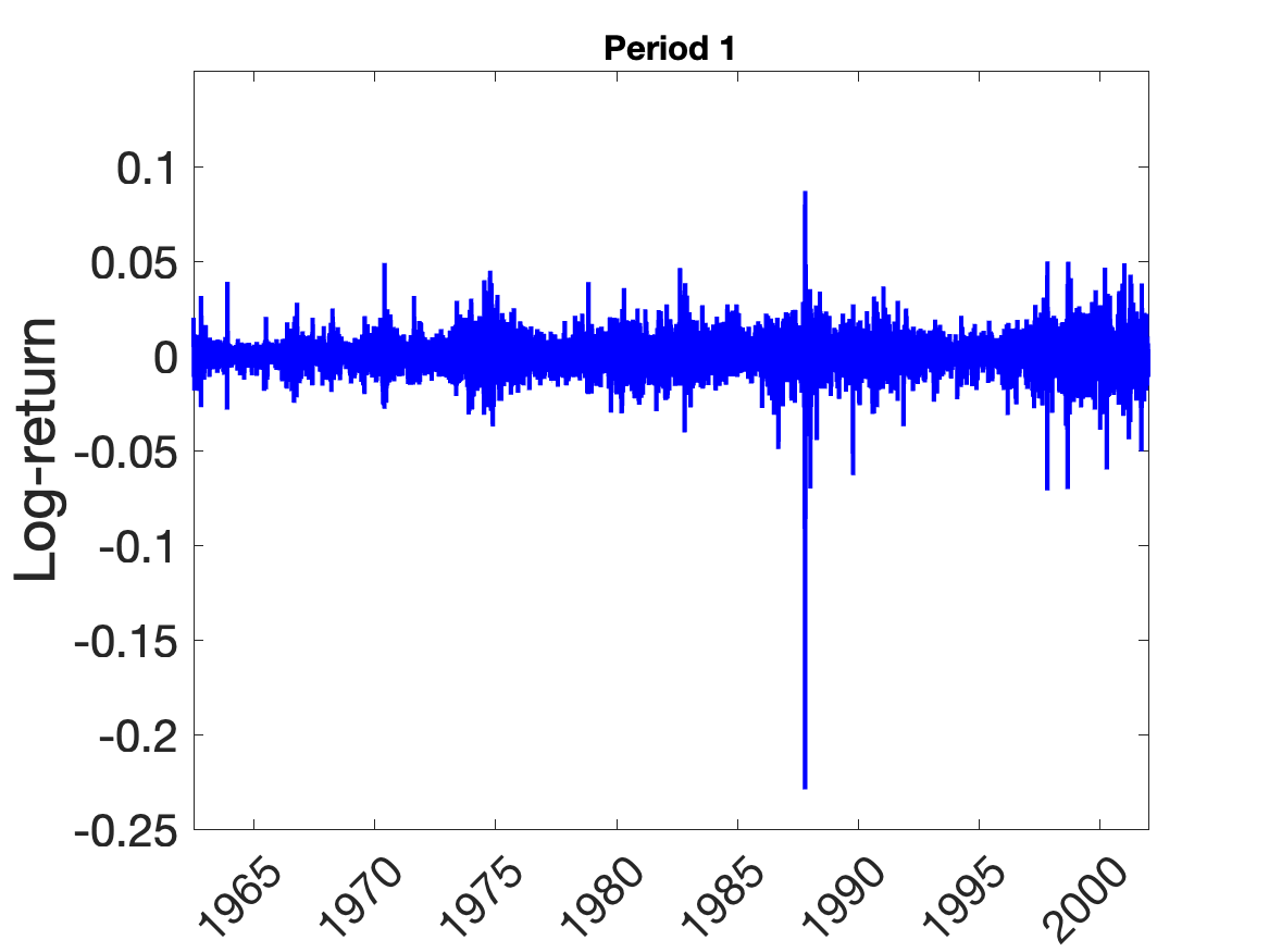
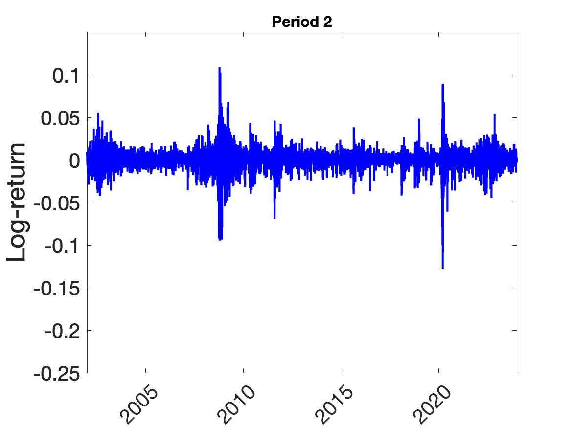
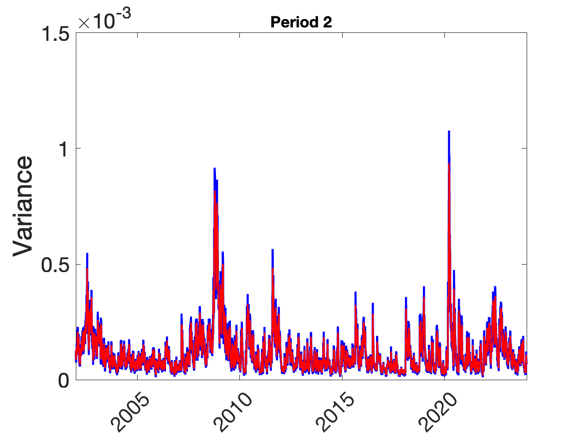
Figure 6: Log-returns S&P 500 series (top panels) and GARCH-CPC model (conditional) variance (bottom panels): $h_{t}$ (blue) and $q_{t}+\bar{h}$ (red) where $\bar{h}={\alpha}/(1-\tilde{\beta}-\alpha\gamma^{2}_{1})$.

As a further comparison, in Figure 7, we display the filtered conditional variance $h_{t}$, the long-term component $q_{t}$, and the short-term component $h_{t}-q_{t}$, as considered by CJOW, for the GARCH-CJOW, GARCH-OP, and GARCH-CPC models. The filtered variances are computed using the parameters from Table 4 for both Period 1 and Period 2. Overall, the filtered variance components of the three models exhibit similar patterns. Moreover, the short-term component $h_{t}-q_{t}$ for the GARCH-OP and GARCH-CPC models is not mean-zero, as explained in Section 3.

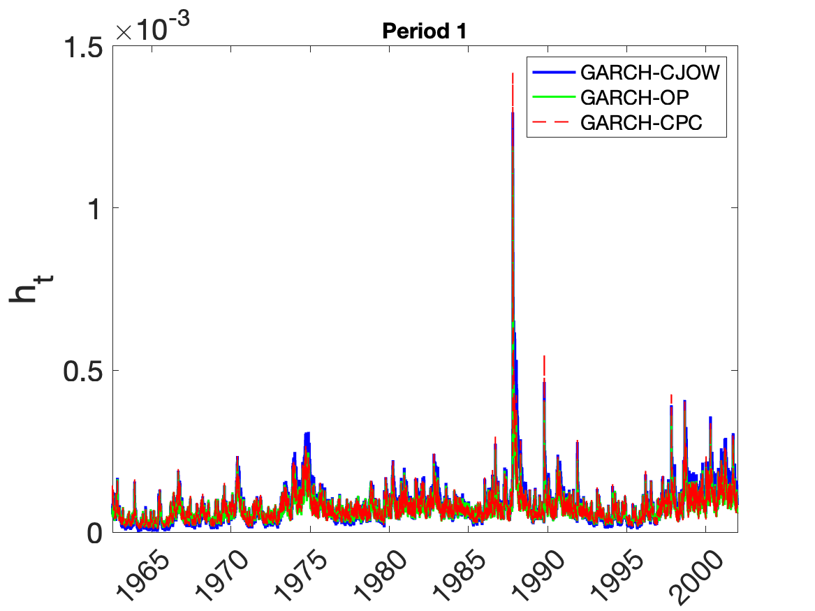
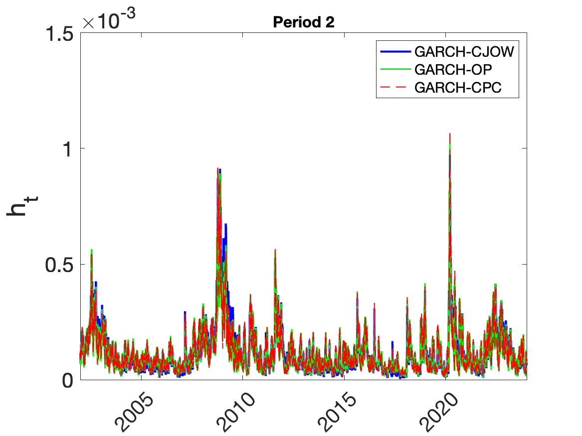
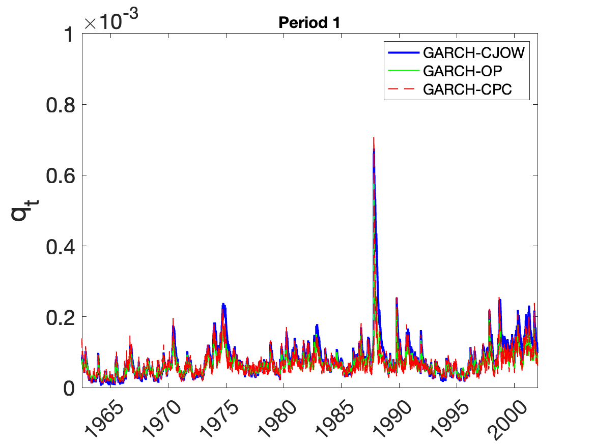
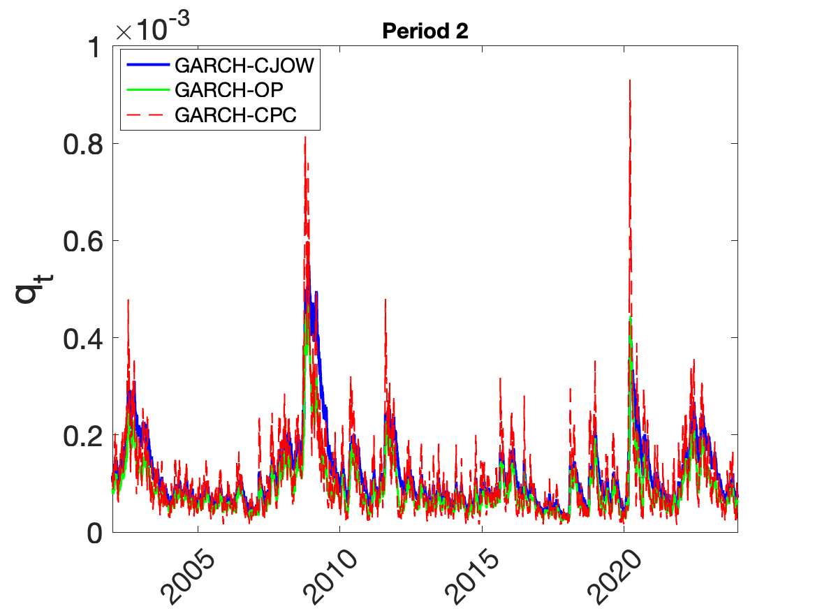
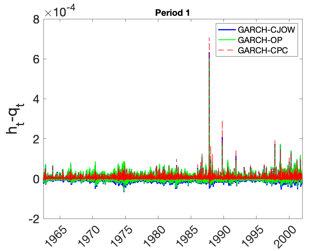
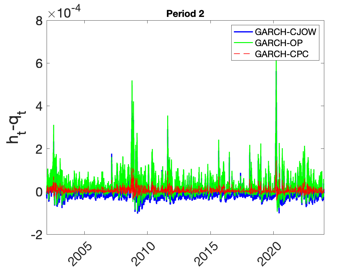
Figure 7: Filtered (conditional) variance.

5 Conclusions

In the influential article by Christoffersen et al. (2008), it is demonstrated that the GARCH-CJOW component model significantly outperforms single component models in capturing stock return volatility. Moreover, the GARCH-CJOW model also shows excellent performance in explaining option prices.

However, a key limitation of the GARCH-CJOW model is its failure to not guarantee positive volatilities, leading to substantial practical challenges. Specifically, even with realistic parameter sets, it is unfeasible to compute option prices for several maturities using the popular semi-closed formula, thereby vanishing one of the main advantages of affine models.

These challenges were partially addressed by the model proposed in Oh and Park (2023). However, as we demonstrate in this paper, it still experiences negative volatilities. Therefore, we propose an enhancement of the GARCH-CJOW and GARCH-OP models, termed GARCH-CPC model, which guarantees the positivity of the variance both theoretically and empirically. Our novel approach demonstrates comparable performance on returns data and superior performance in pricing options compared to both the GARCH-CJOW and GARCH-OP models.

Appendix

Proof of Proposition 1. To obtain the recursive equations for for $A_{t}(\phi)$, $B_{1,t}(\phi)$ and $B_{2,t}(\phi)$ for $t<T$, we use the tower property of the conditional expectation

$$f(t,T;\phi)=\mathbb{E}\left[f(t+1,T;\phi)\middle|\mathcal{F}_{t}\right],$$ (20)

so that by using equation (18) we can express (20) as

$$f(t,T;\phi)=\mathbb{E}\left[e^{\phi\log S_{t+1}+A_{t+1}(\phi)+B_{1,t+1}(\phi)\left(h_{t+2}-q_{t+2}\right)+B_{2,t+1}(\phi)q_{t+2}}\middle|\mathcal{F}_{t}\right].$$ (21)

If we substitute equations (15)-(17) into (21) we obtain

$$f(t,T;\phi)=\mathbb{E}\biggl{[} e^{\phi\left(\log S_{t}+r+\lambda h_{t+1}+\sqrt{h_{t+1}}Z_{t+1}\right)+A_{t+1}(\phi)}$$

$$\times e^{B_{1,t+1}(\phi)\left(\tilde{\beta}(h_{t+1}-q_{t+1})+\alpha\left(Z^{2}_{t+1}+\gamma^{2}_{1}h_{t+1}-2\gamma_{1}\sqrt{h_{t+1}}Z_{t+1}\right)-\alpha\gamma^{2}_{1}q_{t+1}\right)}$$

$$\times e^{B_{2,t+1}(\phi)\left(\omega+\rho q_{t+1}+\varphi\left(Z^{2}_{t+1}+\gamma^{2}_{2}h_{t+1}-2\gamma_{2}\sqrt{h_{t+1}}Z_{t+1}\right)\right)}\biggl{|}\mathcal{F}_{t}\biggr{]}.$$

After re-arranging terms and performing some algebra, we obtain

$$f(t,T;\phi)=\mathbb{E}\biggl{[} e^{\phi(\log S_{t}+r)+\omega B_{2,t+1}(\phi)+A_{t+1}(\phi)}$$ (22)

$$\times e^{\left(\phi\lambda+(\tilde{\beta}+\alpha\gamma^{2}_{1})B_{1,t+1}(\phi)+\varphi\gamma^{2}_{2}B_{2,t+1}(\phi)\right)(h_{t+1}-q_{t+1})+(\phi\lambda+(\rho+\varphi\gamma^{2}_{2})B_{2,t+1}(\phi))q_{t+1}}$$

$$\times e^{\left(\alpha B_{1,t+1}(\phi)+\varphi B_{2,t+1}(\phi)\right)Z^{2}_{t+1}-2\sqrt{h_{t+1}}Z_{t+1}\left(\alpha\gamma_{1}B_{1,t+1}(\phi)+\varphi\gamma_{2}B_{2,t+1}(\phi)-\frac{\phi}{2}\right)}\biggl{|}\mathcal{F}_{t}\biggr{]},$$

so that we can make use of the following result for a standard Normal random variable $Z$:

$$\mathbb{E}\left[e^{aZ^{2}+bZ}\right]=e^{\frac{b^{2}}{2(1-2a)}-\frac{1}{2}\log(1-2a)},\quad a<\frac{1}{2}.$$ (23)

Using (23) and by equating both sides of (22) we obtain:

$$A_{t}(\phi) =A_{t+1}(\phi)+r\phi+B_{2,t+1}(\phi)\omega-\frac{1}{2}\log{(1-2(\alpha B_{1,t+1}(\phi)+\varphi B_{2,t+1}(\phi)))},$$ (24)

$$B_{1,t}(\phi) =B_{1,t+1}(\phi)(\tilde{\beta}+\alpha\gamma^{2}_{1})+\lambda\phi+B_{2,t+1}(\phi)\varphi\gamma^{2}_{2}+2\frac{(\alpha\gamma_{1}B_{1,t+1}(\phi)+\varphi\gamma_{2}B_{2,t+1}(\phi)-\frac{\phi}{2})^{2}}{1-2(\alpha B_{1,t+1}(\phi)+\varphi B_{2,t+1}(\phi))},$$

$$B_{2,t}(\phi) =B_{2,t+1}(\phi)(\rho+\varphi\gamma^{2}_{2})+\lambda\phi+2\frac{(\alpha\gamma_{1}B_{1,t+1}(\phi)+\varphi\gamma_{2}B_{2,t+1}(\phi)-\frac{\phi}{2})^{2}}{1-2(\alpha B_{1,t+1}(\phi)+\varphi B_{2,t+1}(\phi))}.$$

We can use equations (24) to recursively calculate the coefficients starting from $A_{T}(\phi)=0$, $B_{1,T}(\phi)=0$ and $B_{2,T}(\phi)=0$. $\hfill\square$

References

- Christoffersen et al. [2008] P. Christoffersen, K. Jacobs, C. Ornthanalai, and Y. Wang. Option valuation with long-run and short-run volatility components. Journal of Financial Economics, 90(3):272–297, 2008.
- Oh and Park [2023] D.H. Oh and Y.-H. Park. GARCH option pricing with volatility derivatives. Journal of Banking and Finance, 146(2):106718, 2023.
- Engle and Lee [1999] R.F. Engle and G. Lee. A long-run and short-run component model of stock return volatility. In: Engle, R.F. and White, H., Eds., Cointegration, Causality, and Forecasting: A Festschrift in Honor of Clive W.J. Granger. Oxford University Press, pages 475–497, 1999.
- Heston and Nandi [2000] S.L. Heston and S. Nandi. A closed-form GARCH option valuation model. The Review of Financial Studies, 13(3):585–625, 2000.
- Corsi et al. [2013] F. Corsi, N. Fusari, and D. La Vecchia. Realizing smiles: Options pricing with realized volatility. Journal of Financial Economics, 107(2):284–304, 2013.
- Cheng et al. [2023] H-W Cheng, L-H Chang, C-L Lo, and J.T. Tsai. Empirical performance of component GARCH models in pricing VIX term structure and VIX futures. Journal of Empirical Finance, 72:122–142, 2023.
- Bormetti et al. [2015] G. Bormetti, F. Corsi, and A. Majewski. Smile from the past: A general option pricing framework with multiple volatility and leverage components. Journal of Econometrics, 187(2):521–531, 2015.
- Gil-Pelaez [1951] J. Gil-Pelaez. Note on the inversion theorem. Biometrika, 38(3-4):481–482, 1951.
- Christoffersen et al. [2012] P. Christoffersen, K. Jacobs, and C. Ornthanalai. Dynamic jump intensities and risk premiums: Evidence from S&P500 returns and options. Journal of Financial Economics, 106(3):447–472, 2012.
- Ballestra et al. [2023] L.V. Ballestra, E. D’Innocenzo, and A. Guizzardi. Score-driven modeling with jumps: An application to S&P500 returns and options. Journal of Financial Econometrics, 22(2):375–406, 2023.
- Ballestra et al. [2024] L.V. Ballestra, E. D’Innocenzo, and A. Guizzardi. A new bivariate approach for modeling the interaction between stock volatility and interest rate: An application to S&P500 returns and options. European Journal of Operational Research, 314(3):1185–1194, 2024.