Interplay of Tilt and Axion Fields in Topological Superconductors:
Anisotropy in the Meissner Effect

Abstract

The surface states of topological superconductors significantly influence electromagnetic fields within these materials. The interaction between gapless boundary states and electromagnetic fields induces a Berry phase, coupling electric and magnetic fields and introducing the axion term into the effective Lagrangian. In this paper, we utilize a model of a topological superconductor, represented as a “Weyl superconductor-topological insulator-Weyl superconductor” structure with a $\pi$ phase difference between superconductors. By incorporating tilting of Weyl cones, we study the Meissner effect, demonstrating that the interplay between tilt and the axion field enhances surface state contributions. Furthermore, we show that an anisotropy in the Meissner effect arises from the anisotropic nature of the tilt vector. This anisotropy manifests as directional dependence in the magnetic response of the material. We derive a universal equation for magnetic penetration in topological superconductors and explore the impact of tilt on the planar Hall current at the surface.

I Introduction

Topological superconductors are a class of materials that exhibit superconductivity while also possessing unique topological properties Qi and Zhang (2011); Sato and Ando (2017); Sharma et al. (2022); Mandal et al. (2023). These materials are characterized by their ability to host bulk non zero topological numbers alongside featuring gapless boundary states at their edges or surfaces. This makes them promising candidates for fault-tolerant quantum computing Suzuura and Ando (2002); Vijay et al. (2015); Plugge et al. (2016); Chao et al. (2020). A key feature of superconductors, including topological ones, is the Meissner effect. This effect involves the expulsion of magnetic fields from a superconductor’s interior below its critical temperature, highlighting their unique electromagnetic properties Bardeen (1955); Hirsch (2012). In topological superconductors, the Meissner effect not only confirms the superconducting state but also sheds light on the interaction between superconductivity and topologically protected surface statesNogueira et al. (2015); Qi et al. (2013); Stålhammar et al. (2021); Chrispim et al. (2021).

The topological coupling between the electromagnetic field and phase fluctuations of a three-dimensional topological superconductor (3D TSc) bears resemblance to the coupling observed in quantum field theory between an Abelian gauge and axionsNenno et al. (2020). As a result, the electromagnetic response of such a topological superconductor incorporates an axion term, $\sum_{i}C_{1i}\leavevmode\nobreak\ \theta_{i}\leavevmode\nobreak\ \epsilon^{\mu\nu\tau\sigma}F_{\mu\nu}F_{\tau\sigma}$ in which $i$ labels all Fermi surfaces with a Chern number ($C_{1i}$) and $\theta_{i}$ represents the superconducting phase associated with each Fermi surface Qi et al. (2013). The inclusion of the axion term results in an alteration in the equation of motion that dictates the behavior of the magnetic field. Notably, in the vicinity of the surface, the magnetic field behavior converts from a straightforward exponential decay to that of a hypergeometric function - a transformation driven by variations in the axionic field Nogueira et al. (2015).

A theoretical approach to defining a three-dimensional topological superconductor involves considering the proximity of a four-dimensional topological insulator (4D TI) to two trivial s-wave Weyl superconductors (WSc). On the surface of the 4D TI, two thin films of trivial s-wave superconductors become coupled to the TI through the proximity effect and to each other via Josephson coupling. When the two s-wave superconducting films exhibit a $\pi$ phase difference, the resulting Josephson junction serves as a definition for the three-dimensional topological superconductor (3D TSc)Qi et al. (2013).

The well-known TI-Sc heterostructure model, originally proposed by Meng and Balentes in 2012 Meng and Balents (2012), provides an analogous description of the 4D TI model. In this artificially engineered topological superconductivity, the periodicity of the TI-Sc structure replaces the fourth dimension. Specifically, a Sc-TI-Sc structure with a four-dimensional TI is equivalent to an “alternating” Sc-TI-Sc structure with a three-dimensional TI. In both scenarios, achieving a topological superconductor requires that the phase difference between the up and down or left and right superconductors of the TI layer be precisely $\pi$.

We aim to incorporate the tilting of Weyl cones into the theoretical framework of a 3D TSc to observe variations in the electromagnetic responses of the surface states. To achieve this, we assume that the two WScs on opposite sides of the 4D TI model exhibit moderate tilts. We will then investigate how this tilt affects the electromagnetic responses of the entire system.

In the realm of Weyl materials, a particular interest is directed towards those in which the Weyl cones exhibit a preferential tilt within the Brillouin zone, as documented in several studies Tchoumakov et al. (2016); Soluyanov et al. (2015); Koepernik et al. (2016); Belopolski et al. (2016); Wang et al. (2016). The generation of this tilt is often linked to the atomic structure Goerbig et al. (2008); Varykhalov et al. (2017); Ghimire et al. (2019) and also the application of strain or pressure in Weyl semimetalsArjona and Vozmediano (2018); Ferreiros et al. (2019); Liang and Ojanen (2019). We will show that the tilt of Weyl cone plays a significant role in dictating the profile of the axion field near the surface, which in turn affects the magnetic field penetration within topological superconductors. Tilted Weyl semimetals have been predicted to exist in a variety of materials, and was predicted to show a spectrum of properties in the normal phase(non superconducting phase) of the Weyl semimetals, including but not limited to, anisotropy in the planar Hall effect, electrical conductivity, Magnetotransport, Thermal and optical properties, and the Nernst effect Ma et al. (2019); Ahmad and Sharma (2021); Trescher et al. (2015a); Rodionov et al. (2015); Kundu et al. (2020); Ahmad and Sharma (2021); Yadav et al. (2023); Trescher et al. (2015b); Ferreiros et al. (2017); Detassis et al. (2017); Chan et al. (2017); Könye et al. (2023); Jianmei Shao and Yan (2022). However, The focal point of our inquiry is the influence of Weyl cone’s tilt in the superconducting phase. We delve into the tilt impact on the electromagnetic response of a topological superconductor—a phenomenon that remains undetected in trivial superconductivity but becomes apparent through the intermediary of the axion field (evidenced by gapless boundary states on the surface). Thus, we propose that this anisotropy is an axion-mediated phenomena. To confirm our proposition, we have incorporated the Weyl cone tilt as a metric alteration within the Lagrangian framework of the Weyl superconductor Westström and Ojanen (2017); Jalali-Mola and Jafari (2019). We have further concentrated in the consequences of tilting for the magnetic field penetration and the planner Hall effect on the surface of the topological superconductor. The scope of our analysis is confined to moderate tilts, which are characterized by the preservation of a point-like Fermi surface.

We have demonstrated a universal scale-free behavior in the penetration of the magnetic field, applicable across all magnitudes of the tilt vector. This scale invariance feature reveals the limiting behaviour of the magnetic response in topological superconductors.

The paper is organized as follows. Sec. II provides an overview of the axion field in topological superconductors, detailing its computation for systems with a tilted Weyl structure. Sec. III presents the axion field’s profile, incorporating the tilt vector, and also outlines the resulting magnetic field penetration pattern. In Sec. IV, we explore the scale invariance behaviour of the magnetic field with the tilt vector. Sec. V focuses on the anisotropic planner Hall current and we conclude by summarizing our findings in Sec. VI.

II Model and Formulas

In the vicinity of a Weyl point, the Hamiltonian characterizing a tilted Weyl semimetal is given by

$$H_{\chi}=\chi\boldsymbol{\sigma}\cdot\boldsymbol{p}+\sigma_{0}\leavevmode\nobreak\ {\boldsymbol{\zeta}}_{\chi}\cdot\boldsymbol{p},$$ (1)

with $(\sigma_{0},\boldsymbol{\sigma})$ the $2\times 2$ Pauli matrices operating within the spin space. The chirality is denoted by $\chi=\pm$, and ${\boldsymbol{\zeta}}_{\chi}=(\zeta_{x},\zeta_{y})_{\chi}$ is the tilt vector, indexed by $\chi$ to account for the scenarios where the tilts are “towards each other” and “away from each other”

The spontaneously symmetry breaking in quantum field theory can be demonstrated through the theory of a complex scalar field $\phi$ with the Lagrangian,

$$\mathcal{L}=(\partial_{\mu}\phi)^{\dagger}(\partial^{\mu}\phi)-m^{2}\phi^{\dagger}\phi-(\frac{\lambda}{2})(\phi^{\dagger}\phi)^{2}.$$ (2)

In this context, both $m^{2}$ and $\lambda$ in the condensation part, are positive and the stable minima are located at $\phi^{\dagger}\phi=m^{2}/\lambda$. The kinetic term, $(\partial_{\mu}\phi)^{\dagger}(\partial^{\mu}\phi)$ is defined with $\partial^{\mu}\phi:=g^{\mu\nu}\partial_{\nu}\phi$ where $g^{\mu\nu}$ is the inverse of the $4\times 4$ metric tensor of the space-time coordinates. The tilting of Weyl cones introduces a tilt-dependent metric represented by the matrixJalali-Mola and Jafari (2019),

$$g_{\mu\nu}=\begin{pmatrix}1-\zeta^{2}&\zeta_{x}&\zeta_{y}&\zeta_{z}\\ \zeta_{x}&-1&0&0\\ \zeta_{y}&0&-1&0\\ \zeta_{z}&0&0&-1\end{pmatrix},$$ (3)

which in $\boldsymbol{\zeta}=0$ becomes the Minkovski metric $\eta_{\mu\nu}$. Type-I Weyl semimetals are characterized by moderate tilts, $|\zeta|<1$, while type-II ones exhibit over-tilt values, $|\zeta|>1$. The components $\zeta_{x}$, $\zeta_{y}$, and $\zeta_{z}$ represent the tilt projects in the $x$, $y$ and $z$ directions, respectively, with the overall tilt magnitude given by $\zeta=\sqrt{\zeta_{x}^{2}+\zeta_{y}^{2}+\zeta_{z}^{2}}$.

To illustrate topological superconductors in the 4D TI model, the theory involves two order parameters, $\Delta e^{i\theta_{+}}$ and $\Delta e^{i\theta_{-}}$, corresponding to the right and left WScs, respectively. The effective Lagrangian incorporating the axion term that originates from surface states, takes the formQi et al. (2013); Nogueira et al. (2015)

$$\mathcal{L} = \Delta^{2}\sum_{j=\pm}\bigg{[}\partial_{\mu}\theta_{j}(\partial^{\mu}\theta_{j}-qA^{\mu})\bigg{]}+q^{2}\Delta^{2}A_{\mu}A^{\mu}$$

$$+ J\Delta^{2}\cos{(\theta_{+}-\theta_{-})}-m^{2}\Delta^{2}-\frac{\lambda}{2}\Delta^{4}$$

$$- \frac{1}{4}F_{\mu\nu}F^{\mu\nu}-\frac{e^{2}(\theta_{+}-\theta_{-})}{64\pi^{2}}\leavevmode\nobreak\ \epsilon^{\mu\nu\alpha\sigma}F_{\mu\nu}F_{\alpha\sigma},$$

in which the tilt effect is hidden within the contravariant form of electromagnetic field tensor, $F^{\mu\nu}=g^{\mu\alpha}g^{\nu\sigma}F_{\alpha\sigma}$, the contravariant gradient four-vector $\partial^{\mu}=g^{\mu\nu}\partial_{\nu}$, and the vector potential $A^{\mu}=g^{\mu\nu}A_{\nu}$, all defined using the metric (18). The coupling with the electromagnetic sector is achieved through minimal coupling with $q=2e$. We assume $\hbar=c=1$ and reintroduce them as needed. The Josephson term, characterized with coupling strength $J$, arises from the presence of two order parameters with distinct phases, $\theta_{+}$ and $\theta_{-}$. The last term in the Lagrangian, the axion term, plays a significant role in shaping the electromagnetic response of topological superconductors.

By performing a gauge transformation $A_{\mu}\rightarrow A_{\mu}+(1/2q)\partial_{\mu}(\theta_{+}+\theta_{-})$, and changing variables from $(\theta_{+},\theta_{-})$ to $(\theta,\phi)$ where $\theta=(\theta_{+}-\theta_{-})/2$ and $\phi=(\theta_{+}+\theta_{-})/2$, we arrive at a more convenient form for the Lagrangian:

$$\mathcal{L} = \frac{\Delta^{2}}{4}(\partial_{\mu}\theta\partial^{\mu}\theta+4\leavevmode\nobreak\ q^{2}A_{\mu}A^{\mu})$$

$$+ J\Delta^{2}\cos{\theta}-m^{2}\Delta^{2}-\frac{\lambda}{2}\Delta^{4}$$

$$- \frac{1}{4}F_{\mu\nu}F^{\mu\nu}-\frac{e^{2}\theta}{64\pi^{2}}\leavevmode\nobreak\ \epsilon^{\mu\nu\alpha\sigma}F_{\mu\nu}F_{\alpha\sigma}.$$

This transformation clearly shows that while one of the degrees of freedom is gauged away with the electromagnetic field, the other remains within the theory.

We derive the equation of motion for this remaining degree of freedom, termed the ’axion field’, due to its coupling with the electromagnetic field. This coupling mirrors the interaction between the axion field and an Abelian gauge field in quantum field theory Wilczek (1987). Notably, we consider static phase fields, meaning $\partial_{t}\theta_{\pm}=0$ and $\partial^{j}=(-1+\zeta_{j}^{2})\partial_{j}+\sum_{\ell\neq j}\zeta_{j}\zeta_{\ell}\partial_{\ell}$ with $j,\ell=1,2,3$. Consequently, the opposite sign of the $\boldsymbol{\zeta}$ vector for different chiralities is irrelevant.

The Euler-Lagrange equations for the field $\theta$ and the gauge field are given by:

$$\nabla^{2}\theta+\frac{1}{\lambda_{\theta}^{2}}\sin{\theta}=\frac{e^{2}}{4\pi\Delta^{2}}\boldsymbol{E}\cdot\boldsymbol{B}$$ (6a)

$$\partial_{\mu}F^{\mu\nu}+\frac{1}{4\pi^{2}}\epsilon^{\mu\nu\alpha\sigma}F_{\alpha\sigma}\partial_{\mu}\theta=j^{\nu},$$ (6b)

Where $\lambda_{\theta}=1/\sqrt{4J}$ is the penetration depth of the axion field and $j^{\nu}=q\Delta(\partial^{\nu}\phi-2qA^{\nu})$ which under our gauge transformation reduces to $j^{\nu}=-2q\Delta^{2}A^{\nu}$. Importantly, the tilt influences the behaviour of the $\theta$ term and thus the electromagnetic field through the $\nabla^{2}$ operator, a phenomenon observed in topological superconductors but not in trivial (non-topological) ones. Additionally, the tilt parameter affects the electromagnetic field through the upper indices in (6b).

For clarity, we rewrite (6b) for the magnetic field, explicitly showing the role of tilt parameter:

$$(1-\zeta^{2})\boldsymbol{\nabla}\times\boldsymbol{B} = \boldsymbol{\zeta}\times[(\boldsymbol{\zeta}\cdot\boldsymbol{\nabla})\boldsymbol{B}]+(\boldsymbol{\zeta}\cdot\boldsymbol{\nabla})\boldsymbol{E}$$ (7)

$$- q^{2}\Delta^{2}[\boldsymbol{A}-\boldsymbol{\zeta}(\boldsymbol{\zeta}\cdot\boldsymbol{A})]$$

$$+ \frac{e^{2}}{\pi}(\boldsymbol{\nabla}\theta\times\boldsymbol{E}).$$

To provide further intuition, we solve these equations within a simple geometry to highlight the anisotropic behavior of the electromagnetic response. We consider a half-infinite topological superconductor in the region $z>0$, with parallel magnetic ($\boldsymbol{B}_{0}=B_{0}\hat{\boldsymbol{x}}$) and electric ($\boldsymbol{E}_{0}=E_{0}\hat{\boldsymbol{x}}$) fields on the surface and a tilt vector $\boldsymbol{\zeta}=(\zeta_{x},\zeta_{y})$. In this geometry, the Euler-Lagrange equations become:

$$\frac{d^{2}}{dz^{2}}\theta(z)+\frac{1}{\lambda_{\theta}^{2}}\sin\theta(z)=\frac{8e^{2}}{\Delta^{2}}E_{x}B_{x},$$ (8a)

$$-\frac{d^{2}}{dz^{2}}B_{x}+\frac{1}{\lambda_{B}^{2}}B_{x}=-\frac{8e^{2}}{(1-\zeta_{y}^{2})}\frac{d}{dz}(E_{x}\frac{d\theta}{dz}).$$ (8b)

As indicated by equation (8b), the profile of the axion term near the surface significantly influences the magnetic field profile. Consequently, the tilt vector $\boldsymbol{\zeta}$ plays a crucial role in shaping the magnetic field profile and the Meissner effect in topological superconductors. In the absence of the axion term, as in trivial superconductors, Eq. (8b) reduces to a homogeneous differential equation with the trivial solution $\boldsymbol{B}_{0}e^{-z/\lambda_{B}}$, where $\boldsymbol{B}_{0}$ is the magnetic field at the surface. This suggests that $\boldsymbol{\zeta}$ does not affect the electromagnetic response in trivial superconductors lacking the axion term. However, it is noticeable that in our model, the tilt vector has only $x$ and $y$ components. If $\zeta_{z}\neq 0$, the tilt would also affect the magnetic field inside the trivial superconductor as detailed in B: Non-zero $\zeta_{z}$. This effect is present in both trivial and topological superconductors. However, since our focus is on differences caused by surface states, we set $\zeta_{z}=0$.

III Axion and corresponding magnetic fields profiles

The differential equation (8a) approximates the equation of motion for a particle in a tilted washboard potential, represented as $-\zeta_{\theta}\theta+(1/\lambda_{\theta}^{2})\cos\theta$, where $\zeta_{\theta}=8e^{2}E_{x}\ B_{x}/\Delta^{2}$ denotes the potential tilt. Thus, the tilt vector $\boldsymbol{\zeta}$ determines the potential tilt experienced by $\theta$. However, while the tilt of the Weyl cone remains constant, the washboard potential’s tilt for $\theta$ in our model varies with $z$, the distance from the surface.

In this analogy, the solution of (8a) is influenced by the parameter $\zeta_{\theta}$. For small values of $\zeta_{\theta}\leavevmode\nobreak\ (i.e.,|\zeta_{\theta}|<1/\lambda_{\theta}^{2})$, the axion particle is trapped in a local minimum, resulting in $\theta$ taking a constant value of $n\pi$, where $n$ is an integer. The axion field may oscillate around this local minimum (The initial value of $\theta=\pi$ on the surface adds $\pi$ to all subsequent values of $\theta$).

For larger values of $\zeta_{\theta}\leavevmode\nobreak\ (i.e.,|\zeta_{\theta}|>1/\lambda_{\theta}^{2})$, the axion particle escapes these minima, moving freely down the potential slope. Deep within the superconductor, where $z\rightarrow\infty$, and the tilt of the washboard potential approaches zero, $\theta$ assumes a constant value of $2\pi n$ where $n$ is being an integer (considering the initial conditions). This behavior aligns with our understanding of the axion field, which originates from the gapless boundary states and approaches zero (or equivalently $2\pi n$) deep within the topological superconductor.

To streamline the analysis, as suggested in Nogueira et al. (2015), we omit the small non-homogeneous part of the differential equation for $\theta$ and consider the solution of the homogeneous equation adequate: $\theta=\pi+2\arcsin[\tanh(z/\lambda_{\theta})]$. Fig 1 illustrates the variation of $\theta$ with the distance from the surface inside the topological superconductor for different tilt magnitudes. Larger tilts narrow the region of influence of the surface states, resulting in a steeper $\theta$ curve. This steep gradient significantly impacts the magnetic field behavior in this region.

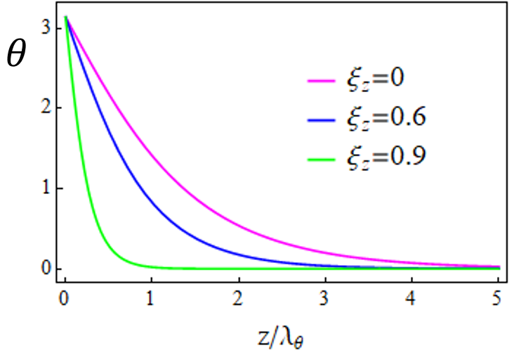
Figure 1: Penetration of the surface states inside the superconductor for different tilt magnitude. For the axion field $\theta$, the values $\theta=0$ and $\theta=2\pi$ are equivalent, both defining trivial (non-topological) superconductivity.

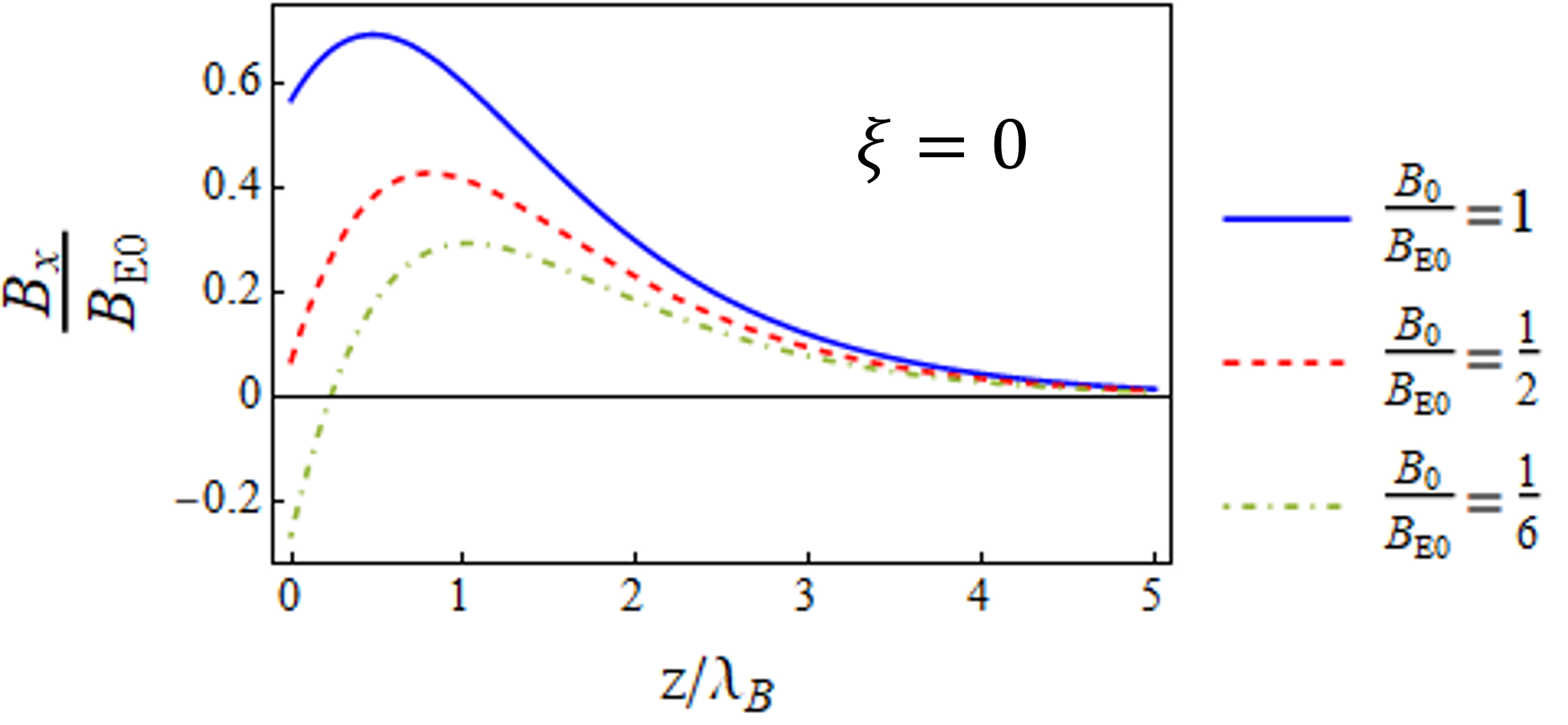
Figure 2: Magnetic field profile in the $x$ direction as a function of $z$, the distance from the surface inside the superconductor, for varying initial values of $B_{x}$ at the surface. Here, $z$ is scaled with $\lambda_{B}$, the penetration depth of the magnetic field, and $B_{x}$ is scaled with $B_{E_{0}}=e^{2}E_{0}/\pi$, where $E_{0}$ is the applied electric field at the surface. The contribution of the axion-mediated electrically induced magnetic field increases with rising $E_{0}$. This enhancement transforms the magnetic field profile from an exponential decay function to a hypergeometric function with a broad peak near the surface.

With the axion field profile established, we can now examine the magnetic field behavior near the surface. In the previously considered geometry, the magnetic field equation is given by:

$$-\frac{d^{2}B_{x}}{dz^{2}}+\frac{1}{\lambda_{B}^{2}}B_{x}=-\frac{e^{2}}{\pi(1-\zeta_{y}^{2})}\frac{d}{dz}(E_{x}\frac{d\theta}{dz}).$$ (9)

This indicates that the tilt affects the magnetic profile via the axion term. For further details on the derivation of (9), refer to A: contravariant vectors in curved space-time.

The analytical solution of this equation is given by:

$$B_{x} = B_{0}e^{-z/\lambda_{B}}$$

$$+ \frac{e^{2}E_{0}\leavevmode\nobreak\ e^{-z/\lambda_{B}}}{\pi(1-\zeta_{y}^{2})}\bigg{\{}\arcsin[\tanh(z/\lambda_{\theta})]$$

$$- \frac{2a}{a+2}e^{-z/\lambda_{\theta}}\leavevmode\nobreak\ _{2}F_{1}(1,\frac{a+2}{2a},\frac{3a+2}{2a},-e^{-2z/\lambda_{\theta}})\bigg{\}}$$

with $a=\frac{\lambda_{\theta}}{\lambda_{B}}$ representing the ratio of the penetration depth of the axion field to the normal penetration depth of the magnetic field. This derivation reveals the existence of two distinct magnetic fields with different origins. The first term denotes the conventional Meissner effect, which occurs in all superconductors. The second term is the axion-mediated magnetic field induced by the electric field, which vanishes in the absence of the applied electric field. It is important to note that the coupling of the axion field with the gauge field is represented by $\theta(\boldsymbol{E}\cdot\boldsymbol{B})$.

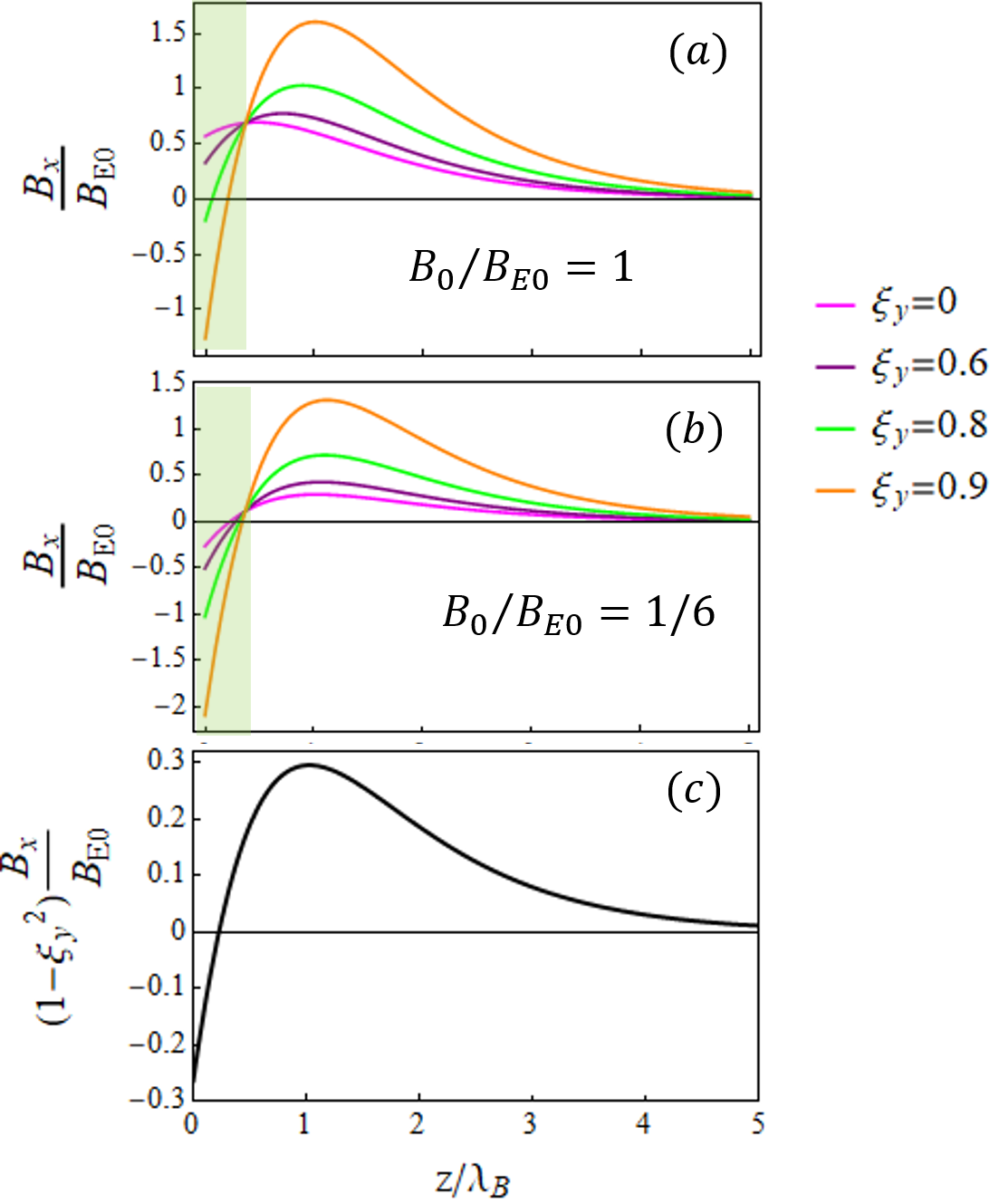
Figure 3: Magnetic field profile in the $x$ direction as a function of $z$ for varying tilt magnitudes. In (a) the initial surface value of $B_{x}$ is $B_{0}=B_{E0}$, while in (b) $B_{0}=(1/6)B_{E0}$. The shaded region highlights the significant differences between the two plots. (c) All data from the panel (b), and additional data for a system with $B_{0}/B_{E_{0}}=1/6$, fall into a universal curve for $(1-\zeta_{y}^{2})B_{x}/B_{E_{0}}$ upon the scaling $z\rightarrow\sqrt{1-\zeta_{y}^{2}}\leavevmode\nobreak\ z$ and $\lambda_{B(\theta)}\rightarrow\sqrt{1-\zeta_{y}^{2}}\leavevmode\nobreak\ \lambda_{B(\theta)}$.

Distinct from the influence of tilting, even if the tilt is zero, in a topological superconductor, the induced magnetic field can disrupt the normal exponential behavior of the Meissner effect if $e^{2}E_{0}/\pi$ is comparable to $B_{0}$. By reintroducing the omitted constants, the ratio becomes $(24\pi^{2}\hbar c\leavevmode\nobreak\ \epsilon_{0}\leavevmode\nobreak\ \mu_{0}/e^{2}(4-\pi))B_{0}/E_{0}$, which is crucial for observing the influence of the induced magnetic field. If this ratio is comparable to or less than unity (see Fig. 2), the alteration in the magnetic field behavior in a topological superconductor is evident. For instance, with electromagnetic radiation, a magnetic field of the order of mT and an electric field of the order of $10^{5}V/m$ results in a ratio of $1/10$, sufficient to observe the axion-mediated magnetic field penetration in the topological superconductor. Notably, a single polarized photon beam with orthogonal magnetic and electric fields is ineffective. At least two orthogonal beams are required to generate parallel electric and magnetic fields.

This explanation provides an intuitive understanding of axion-induced photon interactions, as discussed in Nogueira et al. (2015), which are absent in non-topological superconductors. The Anderson-Higgs mechanism is usually interpreted as the creation of massive photons through the absorption of fluctuations in the phase of the order parameter. However, in topological superconductors, an additional phenomenon occurs. With two phases present, photons absorb the fluctuations of one phase, thereby acquiring mass, while the fluctuations of the other phase induce photon-photon interactions.

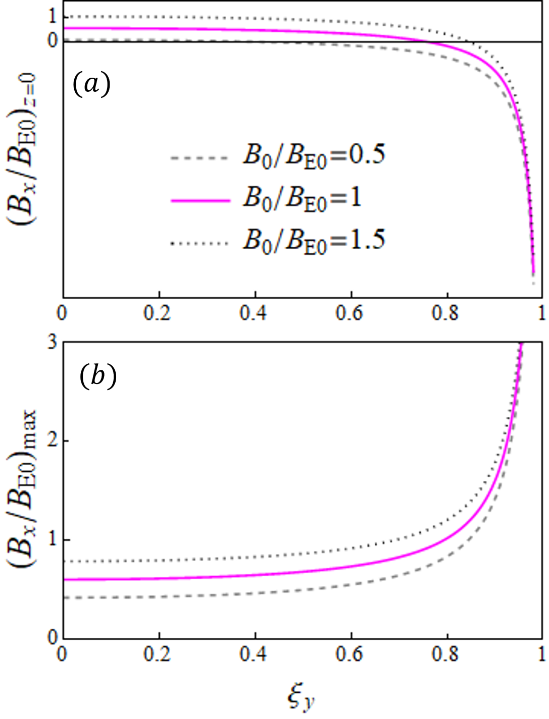
Figure 4: Magnetic field inside the superconductor as a function of $\zeta_{y}$ at $z=0$ and $z=\lambda_{B}$, where $B_{x}$ reaches its maximum value. Various magnitudes of the applied magnetic field are considered. Increasing the applied magnetic field reduces the contribution of the surface states, while tilting enhances this contribution.

Fig. 2 depicts the magnetic field profile near the surface for $\zeta=0$ but varying $B_{0}/E_{0}$ ratios. The dominance of the induced magnetic field, indicative of the axion field’s effectiveness, is contingent upon this ratio. The presence of tilt amplifies the electrically induced magnetic field, enabling it to prevail at lower magnitudes of external electric fields. Fig. 3 (a) and (b), further illustrate the magnetic field penetration profile for a constant $B_{0}/E_{0}$ ratio but varying tilt values. For clarity in comparison, we maintain $\zeta_{x}=0$ and vary $\zeta_{y}$ from $0$ to approximately $1$. As shown, the tilt parameter significantly enhances the effect of the axion field. Another point evident in Fig. 2 (a) and (b) is the increase in the penetration depth of the magnetic field with increasing tilt magnitude. As the tilt grows, the field penetrates deeper into the superconductor, tending to zero at greater distances from the surface.

The ratio $B_{0}/E_{0}$ significantly influences the behavior of the magnetic field in a topological superconductor. However, at a certain threshold, it is the magnitude of the tilt that determines where the exponential behavior is dominated by the induced magnetic field from the external electric field. As the tilt increases, the exponential behavior diminishes progressively. It appears that a larger tilt enhances the influence of surface states, allowing the electromagnetic field to surpass the external magnetic field in dominance. Consequently, in addition to the $B_{0}/E_{0}$ ratio, the magnitude of the tilt emerges as a critical parameter that accentuates the presence of surface states, making them more pronounced.

To illustrate this issue more clearly, in Fig 4, we compare the magnetic field inside the superconductor relative to the tilt magnitude at two critical points for different $B_{0}/E_{0}$ values. The significance of $z=0$ lies in the fact that the external electric field induces a magnetic field in the opposite direction of the external magnetic field due to the presence of surface states at the superconductor’s boundary. If the external electric field is sufficiently large, the resultant of the axion-mediated induced magnetic field and the Meissnerian magnetic field at $z=0$ will oppose the external magnetic field. Fig.4(a) shows that at small tilts, the induced magnetic field is unable to overcome the external magnetic field and alter the magnetic field penetration behavior inside the superconductor. However, as the tilt increases, even with a constant $B_{0}/E_{0}$ value, the intensity of the induced magnetic field increases, causing the trivial Meissner effect behavior to shift to the behavior of a hypergeometric function. The tilt magnitude at which this transition occurs depends on the $B_{0}/E_{0}$ ratio.

In the second part of Figure 4, we plot the value of the magnetic field at the peak of the $B_{x}$ diagram with respect to $z$ as a function of the tilt magnitude. The size of this peak also indicates the magnitude of the induction field. Notably, at point $z=0$, the induced field and the external magnetic field are in opposite directions, whereas at this point, they align. As illustrated in the figure, increasing the tilt at a fixed $B_{0}/E_{0}$ ratio enhances the effect of surface states and the intensity of the induced magnetic field.

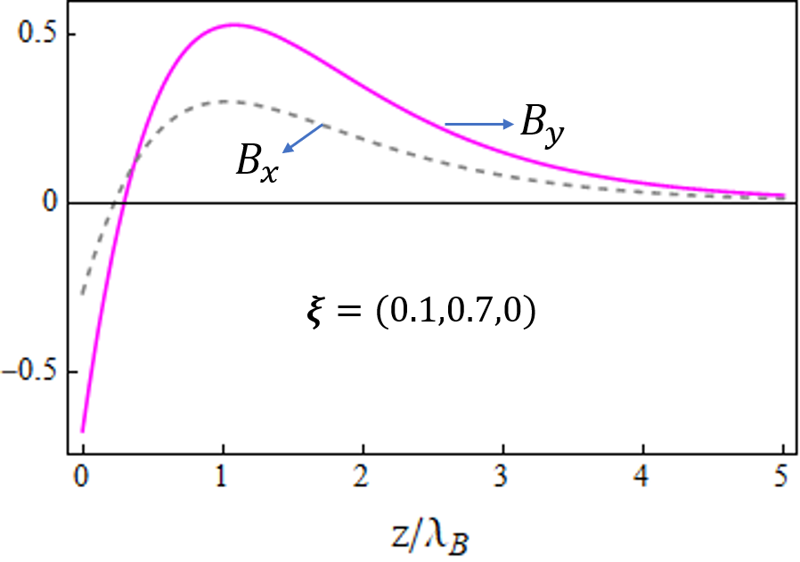
Figure 5: Magnetic field behavior near the surface at $z=0$ in the $x$ and $y$ directions. The tilt vector is $\boldsymbol{\zeta}=(0.1,0.7,0)$. The anisotropic nature of magnetic field penetration is evident.

When the applied magnetic and electric fields are aligned in the $y$-direction, the behavior of $B_{y}$ replicates the previously described phenomena, with $\zeta_{x}$ playing the primary role. This results in anisotropic magnetic field penetration, driven by the directional dependence of the tilt vector. Fig. 5 visualizes this anisotropic penetration profile. As mentioned earlier, such anisotropy is exclusive to topological superconductors. In contrast, ordinary trivial superconductors, even those with tilted Weyl cones, do not display these tilt signatures in the Meissner effect. Consequently, observing this anisotropy serves as evidence of topological superconductivity, with the degree of anisotropy reflecting the ratio of tilt components.

IV Universal Behaviour

As illustrated in Fig. 2 (a) and (b), all the plots for the same $B_{0}/E_{0}$ but different $\zeta_{y}$ share a fixed point that is invariant under the following scaling procedure. Rescaling $z\rightarrow\Lambda z$, $\lambda_{B(\theta)}\rightarrow\Lambda\lambda_{B(\theta)}$, and $B_{x}/E_{0}\rightarrow\Lambda^{2}(B_{x}/E_{o})$ with $\Lambda=\sqrt{1-\xi_{y}^{2}}$ , the differential equation for $B_{x}$ remains invariant under $\zeta_{y}$ variation:

$$-\frac{d^{2}B_{x}}{dz^{2}}+\frac{1}{\lambda_{B}^{2}}B_{x}=-\frac{d}{dz}(e^{-z/\lambda_{B}}\frac{d\theta}{dz}),$$ (11)

thus, the universal magnetic field inside the superconductor now reads:

$$B_{x} = e^{-z/\lambda_{B}}\tilde{B}_{0},$$ (12)

with

$$\tilde{B}_{0} = \bigg{\{}B_{0}+\arcsin[\tanh(z/\lambda_{\theta})]$$

$$- \frac{2a}{a+2}e^{-z/\lambda_{\theta}}\leavevmode\nobreak\ _{2}F_{1}(1,\frac{a+2}{2a},\frac{3a+2}{2a},-e^{-2z/\lambda_{\theta}})\bigg{\}}.$$

These observations lead us to speculate that the universal scaling function (12) applies universally to all curved spaces, demonstrating scale invariance with the tilt vector $\boldsymbol{\zeta}$ (Fig. 3.c).

At the critical value $\zeta_{y}=1$, the relevant lengths $\lambda_{\theta}$ and $\lambda_{B}$ approach zero. Consequently, the influence of surface states on the magnetic field penetration becomes negligible, and the Meissner effect ceases to occur. In this scenario, the topological superconductor with completely expels the applied magnetic field.

V Anomalous PHE and Anisotropic surface current

Building on the derivation of magnetic field behavior from the previous section, we now address the PHE at the boundaries of a topological superconductor. The presence of a non-zero axial term in topological superconductors induces an anomalous Hall effect, characterized by a surface current perpendicular to the applied electric field Nogueira et al. (2015). In our tilted structure, this PHE exhibits pronounced anisotropy attributable to the anisotropic nature of the tilt vector.

The governing equation for the current density $\boldsymbol{j}$ can be derived by obtaining an invariant curl from $j^{\nu}=q\Delta(\partial^{\nu}\phi-2aA^{\nu})$. The use of an invariant curl ensures the correct form, as detailed in A: contravariant vectors in curved space-time. In our simplified model, the expression for $j_{y}$ is obtained as follows:

$$\frac{dj_{y}}{dz}=\frac{1-\zeta_{y}^{2}}{\lambda_{B}^{2}}B_{x}.$$ (14)

which, in universal form, becomes:

$$\frac{dj_{y}}{dz}=\frac{B_{x}}{\lambda_{B}^{2}},$$ (15)

applicable for all tilt values following the convention mentioned earlier.

Revisiting Eq. (14) and following its solution, it is derived that:

$$j_{y} = -\bigg{(}\frac{1-\zeta_{y}^{2}}{\lambda_{B}}\bigg{)}B_{0}e^{-z/\lambda_{B}}$$

$$- \frac{e^{2}E_{0}\leavevmode\nobreak\ e^{-z/\lambda_{B}}}{\pi\lambda_{B}}\bigg{\{}\arcsin[\tanh(z/\lambda_{\theta})]$$

$$+ \frac{2a}{a+2}e^{-z/\lambda_{\theta}}\leavevmode\nobreak\ _{2}F_{1}(1,\frac{a+2}{2a},\frac{3a+2}{2a},-e^{-2z/\lambda_{\theta}})\bigg{\}}.$$

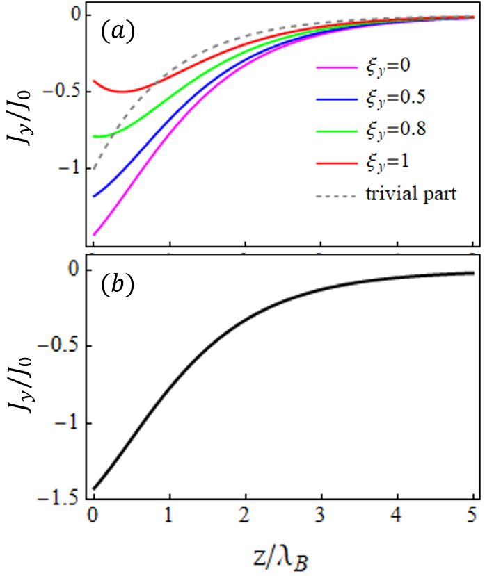
Figure 6: (a) Surface current for $B_{0}=B_{E0}$ with $J_{0}=e^{2}\leavevmode\nobreak\ E_{0}/(\pi\lambda_{B})$. The dashed plot represents the surface current, $-(B_{0}/\lambda_{B})e^{-z/\lambda_{B}}$, in the absence of tilt in a trivial superconductor. The colored plots, each corresponding to different tilt values, depict the total surface current, which includes both the trivial component and the electrically-induced planar Hall current in a topological superconductor.(b) Proper scaling of parameters demonstrates that all curves in panel (a) fall into a universal trend for the surface current upon the scaling $z\rightarrow\Lambda\leavevmode\nobreak\ z$ and $\lambda_{B(\theta)}\rightarrow\Lambda\leavevmode\nobreak\ \lambda_{B(\theta)}$, where $\Lambda=\sqrt{1-\zeta_{y}^{2}}$.

The surface current comprises two components. The first is a conventional term resulting from the exponential decay of the applied magnetic field within the superconductor (indicated by the gray dashed line in Fig. 6, referred to as the trivial current). The second component is the PHE, originating from an electrical source and oriented perpendicular to the applied electric field. This PHE is a consequence of the presence of surface states and is not observed in non-topological superconductors.

The intriguing result is that the tilt parameter now influences the trivial component of the surface current, rather than the axion-mediated component. This leads to a distinct behavior compared to the magnetic field, a phenomenon observable in both trivial and topological superconductors. Notably, the term $1-\zeta_{y}^{2}$ enhances the contribution of the axion-induced planar Hall current. As $\zeta_{y}$ increases from zero to one, the contribution of the first term in (V) diminishes, allowing the axion-mediated part to become more prominent. Fig. 6 (a) illustrates the effect of tilting on the surface current as $\zeta_{y}$ varies from zero to one. At $\zeta_{y}=1$, the current is entirely due to the surface states of the topological superconductor.

In its universal form, the equation for $j_{y}$ becomes:

$$j_{y} = -\bigg{(}\frac{B_{0}}{\lambda_{B}}\bigg{)}e^{-z/\lambda_{B}}$$

$$- \frac{e^{2}E_{0}\leavevmode\nobreak\ e^{-z/\lambda_{B}}}{\pi\lambda_{B}}\bigg{\{}\arcsin[\tanh(z/\lambda_{\theta})]$$

$$+ \frac{2a}{a+2}e^{-z/\lambda_{\theta}}\leavevmode\nobreak\ _{2}F_{1}(1,\frac{a+2}{2a},\frac{3a+2}{2a},-e^{-2z/\lambda_{\theta}})\bigg{\}},$$

which incorporates the tilt effect in $B_{0}$, $\lambda_{B}$, and $z$. Furthermore, $j_{y}\rightarrow j_{y}\sqrt{1-\zeta_{y}^{2}}$. Fig. 6 (b) depicts the universal trend for the surface current upon the scaling $z\rightarrow\Lambda\leavevmode\nobreak\ z$ and $\lambda_{B(\theta)}\rightarrow\Lambda\leavevmode\nobreak\ \lambda_{B(\theta)}$ with $\Lambda=\sqrt{1-\zeta_{y}^{2}}$. Taking the limit $\zeta_{y}=0$ leads to $j_{y}=0$ which is consistent with $B_{x}=0$, resulting in no planar current.

VI Conclusion

In this study, we investigated the axion field-mediated magnetic field and Hall current in topological superconductors. Our primary focus was on the influence of the tilt parameter of the Weyl cone on the features induced in the Meissner effect of surface states, or equivalently, the axion field. As illustrated in Nogueira et al. (2015), the surface states of a topological superconductor couple with the electromagnetic field in a manner similar to the axion field with gauge fields.

We demonstrated that in 4D TI model, the tilt of Weyl cones modifies the penetration depth of surface states inside the 3D topological superconductor and, more importantly, alters the contribution of the electromagnetic-induced field, which is an effect of the surface states. Tilting increases the contribution of surface states in both the magnetic field and planner Hall current.

An intriguing aspect of tilting Weyl cones is the emergence of anisotropy in the Meissner effect, which is absent in non-topological superconductors, even if they are tilted. Additionally, we observed anisotropy in the Hall current on the surface of the tilted topological superconductor, which can be used as a method to determine the ratio of tilt components.

This study underscores the critical role of the tilt parameter in shaping the electromagnetic responses in topological superconductors when model them with 4D TI model. The insights gained from this research enhance our understanding of topological superconductors and open avenues for future investigations into the manipulation of electromagnetic properties for advanced technological applications.

A: contravariant vectors in curved space-time

When the metric tensor is $g_{\mu\nu}$ as illustrated in Eq. (18), the inverse of metric tensor is given by Westström and Ojanen (2017):

$$g^{\mu\nu}=\begin{pmatrix}1&\zeta_{x}&\zeta_{y}&\zeta_{z}\\ \zeta_{x}&-1+\zeta_{x}^{2}&0&0\\ \zeta_{y}&0&-1+\zeta_{y}^{2}&0\\ \zeta_{z}&0&0&-1+\zeta_{z}^{2}\end{pmatrix}.$$ (18)

For example:

$$\partial^{0}=g^{0\nu}\partial_{\nu}=\partial_{t}+\zeta_{x}\partial_{x}+\zeta_{y}\partial_{y}+\zeta_{z}\partial_{z}$$ (19)

and,

$$\partial^{x} = g^{1\nu}\partial_{\nu}$$

$$= \zeta_{x}\partial_{t}+(-1+\zeta_{x}^{2})\partial_{x}+\zeta_{x}\zeta_{y}\partial_{y}+\zeta_{x}\zeta_{z}\partial_{z}.$$

In general, if we denote the gradient in the tilted space as $\overline{\boldsymbol{\nabla}}$ and the gradient in the space with zero tilt as $\boldsymbol{\nabla}$, then:

$$\overline{\boldsymbol{\nabla}}=\boldsymbol{\zeta}\partial_{t}-\boldsymbol{\nabla}-\boldsymbol{\zeta}(\boldsymbol{\zeta}\cdot\boldsymbol{\nabla}),$$ (21)

and similarly for the electromagnetic potential as:

$$\overline{\boldsymbol{A}}=\boldsymbol{\zeta}A_{0}+\boldsymbol{A}-\boldsymbol{\zeta}(\boldsymbol{\zeta}\cdot\boldsymbol{A}).$$ (22)

n the low-frequency regime and in the absence of an electrostatic potential, we set $A_{0}=0$ and $\partial_{t}=0$. By incorporating $\overline{\boldsymbol{A}}$ and $\overline{\boldsymbol{\nabla}}$ into $j^{\nu}$ we obtain:

$$\overline{\boldsymbol{j}}=-2q\Delta^{2}\overline{\boldsymbol{A}}.$$ (23)

Taking the curl and focusing on the $x$-component, we derive:

$$\partial_{y}\overline{\boldsymbol{j}}_{z}-\partial_{z}\overline{\boldsymbol{j}}_{y} = -2q\Delta^{2}(\partial_{y}\overline{\boldsymbol{A}}_{z}-\partial_{z}\overline{\boldsymbol{A}}_{y})$$

$$= -2q\Delta^{2}\bigg{\{}\partial_{y}\big{[}(1-\zeta_{z}^{2})A_{z}-\zeta_{z}\zeta_{x}A_{x}-\zeta_{z}\zeta_{y}A_{y}\big{]}$$

$$- \partial_{z}\big{[}(1-\zeta_{y}^{2})A_{y}-\zeta_{y}\zeta_{x}A_{x}-\zeta_{y}\zeta_{z}A_{z})\big{]}\bigg{\}}.$$

Considering an applied magnetic field in the $x$-direction, we can choose the applied electromagnetic potential as $\boldsymbol{A}=B_{0}z{\hat{j}}$. It is important to note that the derivations are gauge invariant; however, for this step, we adopt this specific form of $\boldsymbol{A}$ to proceed with the equations. With this choice, we have $A_{z}=A_{x}=0$ and $\partial_{y}A_{j}=0$, then:

$$\partial_{y}\overline{\boldsymbol{j}}_{z}-\partial_{z}\overline{\boldsymbol{j}}_{y} = 2q^{2}\Delta^{2}(1-\zeta_{y}^{2})\partial_{z}A_{y}$$

$$= 2q^{2}\Delta^{2}(1-\zeta_{y}^{2})B_{x},$$

where in the last line we use the relation $\boldsymbol{\nabla}\times\boldsymbol{A}=\boldsymbol{B}$. Eq.(A: contravariant vectors in curved space-time) represents the normal curl of the second line of Eq.(7). Next, we aim to obtain the curl of the other terms in this equation:

$$[\boldsymbol{\nabla}\times(\boldsymbol{\zeta}\cdot\boldsymbol{\nabla})\boldsymbol{E}]_{k}=\epsilon_{ijk}\zeta_{\ell}\partial_{j}\partial_{\ell}E_{k},$$ (26)

which is zero because $\boldsymbol{E}$ has derivatives only in the $z$-direction.

For the term $\boldsymbol{\zeta}\times[(\boldsymbol{\zeta}\cdot\boldsymbol{\nabla})\boldsymbol{B}]$, we observe that in our simplified model, $(\boldsymbol{\zeta}\cdot\boldsymbol{\nabla})\boldsymbol{B}=\zeta_{z}\partial_{z}B_{x}\hat{i}$. Consequently, $\boldsymbol{\zeta}\times[(\boldsymbol{\zeta}\cdot\boldsymbol{\nabla})\boldsymbol{B}]=(\zeta_{z}^{2}\hat{j}-\zeta_{y}\zeta_{z}\hat{k})\partial_{z}B_{x}\hat{j}$. The normal curl,$\boldsymbol{\nabla}\times=(\hat{k}\partial_{z})\times$, of this term is$-\zeta_{z}^{2}\partial_{z}^{2}B_{x}\hat{i}$. This term can be combined with $(1-\zeta^{2})\boldsymbol{\nabla}\times\boldsymbol{\nabla}\times\boldsymbol{B}=-(1-\zeta^{2})\partial_{z}^{2}B_{x}\hat{i}$ on the left side of Eq. (6b).

In summary, Eq. (7) simplifies to Eq. (9).

B: Non-zero $\zeta_{z}$

Up to here, we considered the tilt vector as $\boldsymbol{\zeta}=(\zeta_{x},\zeta_{y},0)$ to focus on the aspects of the tilt vector that is crucial in comparing topological and trivial superconductors. However, the presence of $\zeta_{z}$ leads to interesting results worth studying.

If we consider a tilt vector $\boldsymbol{\zeta}=(0,0,\zeta_{z})$ then the term $(\boldsymbol{\zeta}\cdot\boldsymbol{\nabla})\boldsymbol{E}$ in Eq. (7) becomes significant and, independent of the axion field, induces a magnetic field in the transverse direction. Using the same model as mentioned in the main text, Eq. (7) converts to:

$$(1-\zeta^{2})(\boldsymbol{\nabla}\times\boldsymbol{B})_{x} = -\zeta_{z}^{2}\partial B_{y}+\zeta_{z}\partial_{z}E_{x}$$ (27)

$$(1-\zeta^{2})(\boldsymbol{\nabla}\times\boldsymbol{B})_{y} = \zeta_{z}^{2}\partial_{z}B_{x}-q^{2}\Delta^{2}\boldsymbol{A}+\frac{e^{2}}{\pi}E_{x}\partial_{z}\theta.$$

The second line is the same as Eq.(8b) and leads to an axion-mediated induction of the magnetic field, but the first line shows an electromagnetic-induced field that stems directly from tilting and is not due to the surface states:

$$B_{y}=-\leavevmode\nobreak\ \frac{\zeta_{z}E_{0}}{(1-2\zeta_{z}^{2})\lambda_{B}^{2}}e^{-z/\lambda_{B}}.$$ (28)

Contrary to the axion-mediated induced field, this field is in the perpendicular direction to the applied magnetic and electric fields. It is clear that this effect is common between topological and trivial superconductors.

References

- Qi and Zhang (2011) X.-L. Qi and S.-C. Zhang, Rev. Mod. Phys. 83, 1057 (2011).
- Sato and Ando (2017) M. Sato and Y. Ando, Rep. Prog. Phys. 80, 076501 (2017).
- Sharma et al. (2022) M. M. Sharma, P. Sharma, N. K. Karn, and V. P. S. Awana, Supercond. Sci. Technol. 35, 083003 (2022).
- Mandal et al. (2023) M. Mandal, N. C. Drucker, P. Siriviboon, T. Nguyen, A. Boonkird, T. N. Lamichhane, R. Okabe, A. Chotrattanapituk, and M. Li, Chem. Mater. 35, 6184 (2023).
- Suzuura and Ando (2002) H. Suzuura and T. Ando, Phys. Rev. Lett. 89, 266603 (2002).
- Vijay et al. (2015) S. Vijay, T. H. Hsieh, and L. Fu, Phys. Rev. X 5, 041038 (2015).
- Plugge et al. (2016) S. Plugge, L. A. Landau, E. Sela, A. Altland, K. Flensberg, and R. Egger, Phys. Rev. B 94, 174514 (2016).
- Chao et al. (2020) R. Chao, M. E. Beverland, N. Delfosse, and J. Haah, Quantum 4, 352 (2020).
- Bardeen (1955) J. Bardeen, Phys. Rev. 97, 1724 (1955).
- Hirsch (2012) J. E. Hirsch, Phys. Scr 85, 035704 (2012).
- Nogueira et al. (2015) F. S. Nogueira, A. Sudbø, and I. Eremin, Phys. Rev. B 92, 224507 (2015).
- Qi et al. (2013) X.-L. Qi, E. Witten, and S.-C. Zhang, Phys. Rev. B 87, 134519 (2013).
- Stålhammar et al. (2021) M. Stålhammar, M. Stone, M. Sato, and T. H. Hansson, Phys. Rev. B 103, 235427 (2021).
- Chrispim et al. (2021) B. A. S. D. Chrispim, R. C. L. Bruni, and M. S. Guimaraes, Phys. Rev. B 103, 165120 (2021).
- Nenno et al. (2020) C. Nenno, D.M.and Garcia, J. Gooth, C. Felser, and P. Narang, Nat. Rev. Phys. 2, 682 (2020).
- Meng and Balents (2012) T. Meng and L. Balents, Phys. Rev. B 86, 054504 (2012).
- Tchoumakov et al. (2016) S. Tchoumakov, M. Civelli, and M. O. Goerbig, Phys. Rev. Lett. 117, 086402 (2016).
- Soluyanov et al. (2015) D. Soluyanov, A.and Gresch, Z. Wang, Q. Wu, M. Troyer, X. Dai, and B. A. Bernevig, Nature 527, 495 (2015).
- Koepernik et al. (2016) K. Koepernik, D. Kasinathan, D. V. Efremov, S. Khim, S. Borisenko, B. Büchner, and J. van den Brink, Phys. Rev. B 93, 201101 (2016).
- Belopolski et al. (2016) I. Belopolski, S.-Y. Xu, Y. Ishida, X. Pan, P. Yu, D. S. Sanchez, H. Zheng, M. Neupane, N. Alidoust, G. Chang, T.-R. Chang, Y. Wu, G. Bian, S.-M. Huang, C.-C. Lee, D. Mou, L. Huang, Y. Song, B. Wang, G. Wang, Y.-W. Yeh, N. Yao, J. E. Rault, P. Le Fèvre, F. m. c. Bertran, H.-T. Jeng, T. Kondo, A. Kaminski, H. Lin, Z. Liu, F. Song, S. Shin, and M. Z. Hasan, Phys. Rev. B 94, 085127 (2016).
- Wang et al. (2016) C. Wang, Y. Zhang, J. Huang, S. Nie, G. Liu, A. Liang, Y. Zhang, B. Shen, J. Liu, C. Hu, Y. Ding, D. Liu, Y. Hu, S. He, L. Zhao, L. Yu, J. Hu, J. Wei, Z. Mao, Y. Shi, X. Jia, F. Zhang, S. Zhang, F. Yang, Z. Wang, Q. Peng, H. Weng, X. Dai, Z. Fang, Z. Xu, C. Chen, and X. J. Zhou, Phys. Rev. B 94, 241119 (2016).
- Goerbig et al. (2008) M. O. Goerbig, J.-N. Fuchs, G. Montambaux, and F. Piéchon, Phys. Rev. B 78, 045415 (2008).
- Varykhalov et al. (2017) A. Varykhalov, D. Marchenko, J. Sánchez-Barriga, E. Golias, O. Rader, and G. Bihlmayer, Phys. Rev. B 95, 245421 (2017).
- Ghimire et al. (2019) M. P. Ghimire, J. I. Facio, J.-S. You, L. Ye, J. G. Checkelsky, S. Fang, E. Kaxiras, M. Richter, and J. van den Brink, Phys. Rev. Res. 1, 032044 (2019).
- Arjona and Vozmediano (2018) V. Arjona and M. A. H. Vozmediano, Phys. Rev. B 97, 201404 (2018).
- Ferreiros et al. (2019) Y. Ferreiros, Y. Kedem, E. J. Bergholtz, and J. H. Bardarson, Phys. Rev. Lett. 122, 056601 (2019).
- Liang and Ojanen (2019) L. Liang and T. Ojanen, Phys. Rev. Res. 1, 032006 (2019).
- Ma et al. (2019) D. Ma, H. Jiang, H. Liu, and X. C. Xie, Phys. Rev. B 99, 115121 (2019).
- Ahmad and Sharma (2021) A. Ahmad and G. Sharma, Phys. Rev. B 103, 115146 (2021).
- Trescher et al. (2015a) M. Trescher, B. Sbierski, P. W. Brouwer, and E. J. Bergholtz, Phys. Rev. B 91, 115135 (2015a).
- Rodionov et al. (2015) Y. I. Rodionov, K. I. Kugel, and F. Nori, Phys. Rev. B 92, 195117 (2015).
- Kundu et al. (2020) A. Kundu, Z. Bin Siu, Y. H., and M. B. A. Jalil, New J. Phys. 22, 083081 (2020).
- Yadav et al. (2023) S. Yadav, S. Sekh, and I. Mandal, Physica B: Cond. Matt. 656, 414765 (2023).
- Trescher et al. (2015b) M. Trescher, B. Sbierski, P. W. Brouwer, and E. J. Bergholtz, Phys. Rev. B 91, 115135 (2015b).
- Ferreiros et al. (2017) Y. Ferreiros, A. A. Zyuzin, and J. H. Bardarson, Phys. Rev. B 96, 115202 (2017).
- Detassis et al. (2017) F. Detassis, L. Fritz, and S. Grubinskas, Phys. Rev. B 96, 195157 (2017).
- Chan et al. (2017) C.-K. Chan, N. H. Lindner, G. Refael, and P. A. Lee, Phys. Rev. B 95, 041104 (2017).
- Könye et al. (2023) V. Könye, L. Mertens, C. Morice, D. Chernyavsky, A. G. Moghaddam, J. van Wezel, and J. van den Brink, Phys. Rev. B 107, L201406 (2023).
- Jianmei Shao and Yan (2022) J. Jianmei Shao and L. Yan, Journal of Physics: Cond. Matt. 35, 025401 (2022).
- Westström and Ojanen (2017) A. Westström and T. Ojanen, Phys. Rev. X 7, 041026 (2017).
- Jalali-Mola and Jafari (2019) Z. Jalali-Mola and S. A. Jafari, Phys. Rev. B 100, 205413 (2019).
- Wilczek (1987) F. Wilczek, Phys. Rev. Lett. 58, 1799 (1987).