Mimetic Metrics for the DGSEM
Abstract
Free-stream preservation is an essential property for numerical solvers on curvilinear grids. Key to this property is that the metric terms of the curvilinear mapping satisfy discrete metric identities, i.e., have zero divergence. Divergence-free metric terms are furthermore essential for entropy stability on curvilinear grids. We present a new way to compute the metric terms for discontinuous Galerkin spectral element methods (DGSEMs) that guarantees they are divergence-free. Our proposed mimetic approach uses projections that fit within the de Rham Cohomology.
Keywords:
Free-Stream Preservation, Mimetic Methods, Discontinuous Galerkin, Divergence Free Methods, Curved MeshesMSC:
65Mxx1 Introduction
We focus on discontinuous Galerkin spectral element methods (DGSEMs) for conservation laws of the form
| (1) |
on a domain , where the conserved variable is , are the flux functions and denotes the divergence operator in physical space. To solve the conservation law numerically we partition with a conforming quadrilateral or hexahedral mesh. We require the global mapping to be inside each cell and both mapping and normal vectors to be continuous across cell interfaces. Let be the mapping from the reference element to an element in the physical domain.
After the conservation law is transformed to the reference element, it reads
| (2) |
where is the mapping Jacobian and are the metric terms,
| (3) |
with the canonical space unit vectors .
If we consider a constant state and its corresponding constant flux , with constant or periodic boundary conditions, we get from equation (2) the time derivative
| (4) |
where we used the fact that for the analytical global mapping with the conditions specified the divergence of the metric terms is zero - the constant state stays constant in time.
For the DGSEM (see, e.g., Kopriva (2006)), we use a tensor product ansatz and interpolate and the flux functions with polynomials of degree in each direction. Let be the tensor product interpolation operator and the tensor product Lagrange polynomials. We use integration-by-parts, replace the boundary flux with the numerical flux, use the summation-by-parts property and collocate interpolation and quadrature using Legendre-Gauss-Lobatto (LGL) nodes to arrive at the strong form of the DGSEM,
| (5) |
for all multi-indices . Here the subscript i denotes the value of the function at the corresponding grid point, is the reference element, is the product of the LGL quadrature weights at the corresponding grid point and denotes the numerical LGL-quadrature of the boundary integral (see Kopriva (2006)).
Substituting the constant state into the DGSEM, the boundary term cancels due to the consistency of the numerical flux and we get
| (6) |
which is zero when the divergence of the discrete metric terms is zero
| (7) |
Even if the mapping x is polynomial, the metric terms are of a higher polynomial order. For the interpolation operator to still act as the identity operator in (7), we would have to restrict the mapping order to . A different approach is used in Kopriva (2006) where the metric terms are computed as
| (8) |
Since we now take the analytical curl of the interpolation and the divergence of a curl is zero, the curl form approximation of the metric terms guarantees free-stream preservation.
2 Mimetic Approach
An alternative the curl form of Kopriva (2006) is the use of mimetic projections coming from finite element exterior calculus Arnold DN (2006). We first look at the dual de Rham chain complex in 3D, and choose for each space a finite dimensional subspace and projections . We use the dual complex since in 2D the divergence operator is not part of the de Rham cochain complex, which has the following commuting diagram:
Since we work with quadrilateral or hexahedral elements and use a tensor product ansatz, we follow the work of Gerritsma Gerritsma (2011) and define the spaces as
| (9) | ||||
| (10) | ||||
| (11) | ||||
| (12) |
in the reference element, where and stand for the spaces of one-dimensional polynomials of up to degree or , respectively. We further require continuity across element boundaries in the direction that has polynomial degree . We note that these continuity requirements couple the nodal degrees of freedom similar to a continuous finite element approach. Gerritsma Gerritsma (2011) also presents specific basis functions based on Lagrange polynomials with LGL nodes and their corresponding histopolation bases for an implementation.
For the projection operators we give the first component of as an example,
| (13) |
where the are the 1D Lagrange polynomials and is defined by
| (14) |
Here, we take line integrals between the LGL points in the direction that is discontinuous and interpolate in the other directions.
The other projections are defined analogously.
With the conditions on the mesh and mapping, the metric terms, are in , while the potential lives in .
As the diagram commutes, we are allowed to follow different paths. Hence, we have two options with which to construct the discrete metric terms that result in the same approximation (up to machine precision).
Option red: We project directly via to get
| (15) |
Option blue: We project via to get . We compute the metric terms by applying the curl, i.e.
| (16) |
It then holds that
| (17) |
by construction, which gives free-stream preservation.
Remark 1
To compute (15) or (16), we require exact integration of the mapping terms to compute the projections onto the histopolation bases, which can be achieved by using a quadrature rule with enough points to achieve errors on the order of machine precision, if calculation by hand is impractical or impossible. We also require exact derivatives of the mappings in (15) or (16), and exact derivatives of the potential in (15), which can be found using automatic differentiation. We note, in case no analytic global mapping is available or is inconvenient, the common pre-processing step of approximating the geometry with a piece-wise polynomial ansatz can be used instead.
Remark 2
In 2D, the approach in Kopriva (2006) is to interpolate the mapping components and then take the analytic 2D curl to achieve free-stream preservation. This approach is equivalent to the mimetic approach because the metric terms in 2D depend linearly on the mapping components, i.e., (3) reduces to
| (18) |
and with the conditions on the mapping, . In other words, for 2D we have the smaller commuting diagram
where . The approach for 2D in Kopriva (2006) is equivalent to taking the blue path.
3 Numerical Example
As an example, we discretize the linear advection equation
| (19) |
and use the mapping
| (20) | ||||
| (21) | ||||
| (22) |
from the reference domain with
| (23) |
and end time . We use a conforming mesh with two elements in each direction and periodic boundary conditions.
Simulations are done with a slightly modified version of the DGSEM code of the Julia package Trixi.jl (see Ranocha et al. (2022) and Schlottke-Lakemper et al. (2021)) performed on a Macbook Pro M2, single thread, with MacOS 14.5. A reproducibility repository can be accessed under https://github.com/amrueda/paper_2024_mimetic_metrics.
We examine both free-stream preservation and the approximation of the analytic metric terms by varying the polynomial degree up to for both the curl form by Kopriva in Kopriva (2006) and the mimetic variant. Both errors are measured in the and the norm. The norms are computed numerically using integration with 51 points in each direction in every element for the norm, and by the minimum of the point value errors on the same points as the discrete evaluation of the norm.
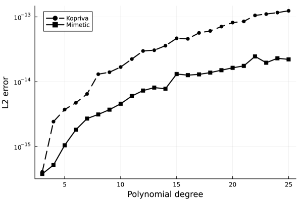
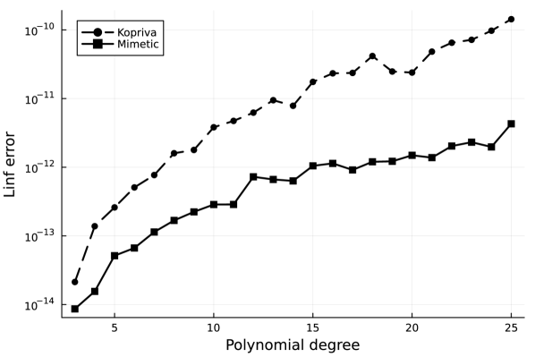
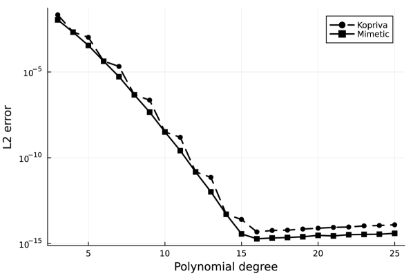
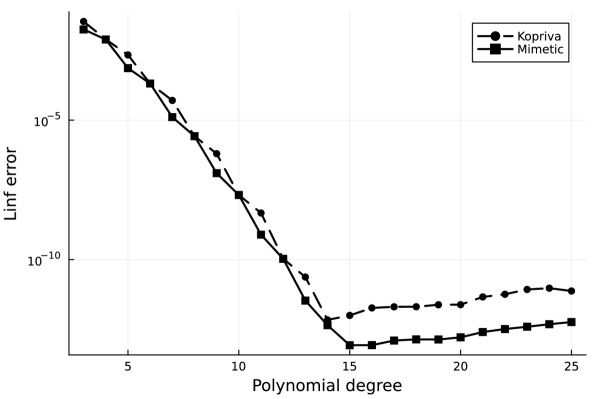
In Fig. 1(a) and 1(b) we can see that free-stream preservation is achieved with both the curl and the mimetic approach, and that the machine precision errors grow with increasing polynomial degree for both. We also observe that the mimetic approach has lower machine precision error than Kopriva’s curl form by over an order of magnitude in the norm. In Figure 2(a) and 2(b) we see convergence of the contravariant vectors to machine precision, though the machine errors are again higher for Kopriva’s approximation.
4 Conclusion
We have constructed an alternative way to compute the metric terms for the DGSEM scheme in a divergence-free way via a mimetic approach using de Rham dual complexes for both two and three space dimensions. In two space dimensions the method of Kopriva (2006) and the mimetic approach are analytically the same, but they differ in three dimensions. Both approaches do obtain free-stream preservation for conforming meshes and exhibit a similar convergence behavior for the contravariant vectors. However, in all cases the mimetic approach has better rounding error properties. We remark that the finite element exterior calculus projections do not only exist for quadrilateral or hexahedral meshes but also, for example, for triangular or tetrahedral meshes Arnold DN (2006).
5 Acknowledgements
This work was supported by a grant from the Simons Foundation (#426393, #961988, David Kopriva). Gregor Gassner and Andrés M. Rueda-Ramírez acknowledge funding through the Klaus-Tschira Stiftung via the project “HiFiLab” (00.014.2021) and through the German Federal Ministry for Education and Research (BMBF) project “ICON-DG” (01LK2315B) of the “WarmWorld Smarter” program. Gregor Gassner and Daniel Bach acknowledge funding from the German Science Foundation DFG through the research unit “SNuBIC” (DFG-FOR5409).
References
- Arnold DN (2006) Arnold DN, Falk RS, W.R., 2006. Finite element exterior calculus, homological techniques, and applications. Acta Numerica 15, 1–155. doi:https://doi.org/10.1017/S0962492906210018.
- Gerritsma (2011) Gerritsma, M., 2011. Edge Functions for Spectral Element Methods, in: Hesthaven, J.S., Rønquist, E.M. (Eds.), Spectral and High Order Methods for Partial Differential Equations, Springer Berlin Heidelberg, Berlin, Heidelberg. pp. 199–207. doi:https://doi.org/10.1007/978-3-642-15337-2_17.
- Kopriva (2006) Kopriva, D., 2006. Metric Identities and the Discontinuous Spectral Element Method on Curvilinear Meshes. Journal of Scientific Computing 26, 301–327. doi:https://doi.org/10.1007/s10915-005-9070-8.
- Ranocha et al. (2022) Ranocha, H., Schlottke-Lakemper, M., Winters, A.R., Faulhaber, E., Chan, J., Gassner, G., 2022. Adaptive numerical simulations with Trixi.jl: A case study of Julia for scientific computing. Proceedings of the JuliaCon Conferences 1, 77. doi:https://doi.org/10.21105/jcon.00077, arXiv:2108.06476.
- Schlottke-Lakemper et al. (2021) Schlottke-Lakemper, M., Gassner, G.J., Ranocha, H., Winters, A.R., Chan, J., 2021. Trixi.jl: Adaptive high-order numerical simulations of hyperbolic PDEs in Julia. https://github.com/trixi-framework/Trixi.jl. doi:https://doi.org/10.5281/zenodo.3996439.