Air Resistance From the Acceleration of a Falling Smartphone

Abstract

This study investigates the motion of a falling smartphone under the influence of air drag using acceleration data collected by its built-in accelerometer. By analyzing the proper acceleration profiles, we could distinguish between laminar and turbulent drag regimes, a distinction readily apparent even through visual inspection of the data. The turbulent drag model proves to be a suitable representation for the observed motion, accurately capturing the dynamics of both the upward and downward phases of the smartphone’s flight. This approach provides an effective and simple method to explore fluid dynamics concepts in an educational context.

1 Introduction

The study of falling objects under the influence of air resistance is a common topic in introductory experimental physics courses [1, 2, 3], providing valuable insights into the interplay between gravitational forces and fluid dynamics. However, accurately modeling air drag presents challenges due to the numerous variables involved, such as the object’s shape, size, orientation, velocity, and the properties of the surrounding fluid [4]. These factors make air resistance a nuanced subject with both theoretical and practical relevance.

The intricate nature of air-object interactions gave rise to the specialized field of aerodynamics [5]. This area often relies on advanced tools such as wind tunnels and supercomputers to tackle its demanding problems. Nevertheless, in basic physics courses, air drag is addressed through simplifications. Such simplifications are useful in educational contexts, as they provide manageable models that still capture the essence of practical scenarios. Following this strategy, two models are typically introduced: laminar and turbulent flows [6].

A straightforward way to explore these models experimentally is by filming falling objects and analyzing their position-time data using video analysis software [7]. Although this method is both intuitive and accessible, it has limitations in distinguishing between drag regimes, since laminar and turbulent flows produce similar position-time profiles.

To overcome these limitations, we propose using smartphones’ built-in accelerometers to measure proper acceleration during their fall. This method provides a key advantage: differences between laminar and turbulent drag become evident in the acceleration profiles, even through simple visual inspection. As a result, it allows for a more precise identification of the drag regime acting on the object.

This method also offers valuable educational opportunities by providing a simple experimental setup—dropping the smartphone—which facilitates the exploration of real data and fundamental physical concepts. The inherent variability in experimental conditions, such as initial velocities, tilt, or potential rotations of the phone, emphasizes the role of experimental uncertainties and the importance of repeated measurements. These features offer a comprehensive view of the experimental process, emphasizing hands-on experimentation, data selection and analysis, and the integration of modern technology.

Our results demonstrate that acceleration data collected via smartphones can effectively distinguish between laminar and turbulent drag regimes. While the laminar flow model does not adequately describe the observed data, the turbulent flow model provides a much better fit. Despite the inherent complexities of air drag, these simple smartphone-based acceleration measurements, combined with turbulent flow modeling, provide valuable insights, even with the variability introduced by manual drops.

The remainder of this paper is organized as follows: Section 2 presents the theoretical model for the smartphone’s motion under air resistance, covering laminar and turbulent regimes. Section 3 describes the experimental setup and data collection using the smartphone’s accelerometer. In Section 4, we outline the methodology and present the results. Section 5 discusses the findings and the effectiveness of the experimental approach. Section 6 explores potential future research directions, and the appendix A provides the estimation of the drag coefficient.

The analysis code (written in Python using NumPy, Matplotlib, and SciPy) and experimental data from this study are available on GitHub at this repository.

2 Drag Model

As the smartphone moves through the air, it experiences a drag force given by:

$$\vec{F}_{D}=k|\vec{v}_{p}|^{n}\vec{v}_{p},$$ (1)

where $k$ is a constant that depends on the object’s shape, size, orientation, and the fluid’s properties, and $n$ is an exponent characterizing the flow regime: $n=0$ for laminar flow and $n=1$ for turbulent flow. The term $\vec{v}_{p}$ denotes the velocity of the air in the smartphone’s reference frame. This formulation differs from the conventional drag force, which considers the object’s velocity relative to the medium and includes a negative sign.

To model the air velocity in the smartphone’s frame, $\vec{v}_{p}$, we apply Newton’s second law in an inertial reference frame fixed to the Earth’s surface. This is necessary because the accelerating smartphone constitutes a non-inertial frame. We make the following assumptions:

• The $z$-axis points upward in the Earth frame.

• The smartphone’s motion is purely vertical in this frame, i.e., $\vec{v}=v\hat{z}$.

• The air is stationary with respect to the Earth.

• The smartphone’s screen faces upward, so $\hat{z}\cdot\hat{z}_{p}=1$, where $\hat{z}_{p}$ denotes the unit vector perpendicular to the smartphone’s screen [8].

Under these conditions, $\vec{v}_{p}=-\vec{v}$.

With this setup, Newton’s second law, in the Earth’s reference frame, provides the following smartphone’s acceleration:

$$a=-g-\frac{k}{m}|v|^{n}v,$$ (2)

where $g$ is the acceleration due to gravity, and $m$ is the mass of the smartphone. This equation can be expressed in terms of the smartphone’s proper acceleration, $a_{p}$, which is the acceleration measured by the accelerometer:

$$a=-g+a_{p},$$ (3)

where

$$a_{p}=\frac{F_{D}}{m}=-\frac{k}{m}|v|^{n}v.$$ (4)

This proper acceleration, $a_{p}$, serves as our model for the accelerometer readings.

From Eq. (2), we can derive an important consequence of air resistance during fall: the existence of a finite terminal velocity. As an object falls, the drag force increases with velocity. Eventually, the drag force equals the gravitational force, resulting in zero net acceleration and constant velocity. This equilibrium velocity is known as the terminal velocity and is defined as:

$$|v_{t}|^{n}v_{t}=-\frac{mg}{k}.$$ (5)

The negative sign indicates downward motion at terminal velocity. For simplicity, we define $v_{t}$ to be positive. This allows us to express the terminal speed as:

$$v_{t}=\left(\frac{mg}{k}\right)^{\frac{1}{n+1}}.$$ (6)

In this work, we choose to use the terminal velocity $v_{t}$ as a free parameter instead of the drag coefficient $k$. This choice is advantageous because $v_{t}$ is more directly measurable and intuitive than $k$. By substituting the expression for $v_{t}$ into the previous equations, we can rewrite the acceleration terms as:

$$a =-g\left(1+\frac{|v|^{n}v}{v_{t}^{n+1}}\right),$$ (7)

$$a_{p} =-g\frac{|v|^{n}v}{v_{t}^{n+1}}.$$ (8)

These expressions clearly show the relationship between the velocity $v$ and the terminal velocity $v_{t}$, highlighting that as the velocity approaches $-v_{t}$, the total acceleration $a$ approaches zero. The proper acceleration $a_{p}$ reflects only the effects of air drag. As $v$ approaches $-v_{t}$, $a_{p}$ approaches $g$, creating an accelerated frame that, from the perspective of the accelerometer, is equivalent to being at rest in Earth’s gravitational field.

Our theoretical framework for analyzing the smartphone’s fall is encapsulated in these two equations: Eq. (7) describes the acceleration in the Earth-based inertial frame, providing its velocity $v$, while Eq. (8) represents the proper acceleration as measured in the smartphone’s own reference frame. Together, these two equations form the foundation for interpreting the accelerometer data collected during our experiments.

2.1 Laminar Flow

For laminar flow, which typically occurs at low velocities and with small objects [4], the drag force is proportional to velocity. This proportionality can be represented by setting $n=0$ in our general drag force, given by Eq.(1). By integrating the acceleration in the Earth-based reference frame, Eq.(7), we find the velocity under these conditions:

$$v(t)=-v_{t}\left(1-\text{e}^{-\frac{g}{v_{t}}t}\right)+v_{0}\,\text{e}^{-\frac{g}{v_{t}}t}.$$ (9)

Here, $v_{0}$ is the initial velocity. Note that the terminal velocity is $v(t\rightarrow\infty)=-v_{t}$, regardless of $v_{0}$, indicating that the object eventually reaches the same terminal velocity irrespective of its initial speed.

In cases where the initial velocity is upward $(v_{0}>0)$, it is useful to determine the time at which the object reaches its maximum height, denoted as $t_{\text{apex}}$. The apex occurs when the vertical velocity momentarily becomes zero, $v(t_{\text{apex}})=0$. Using our derived expression for $v(t)$, we have:

$$t_{\text{apex}}=\frac{v_{t}}{g}\ln\left(1+\frac{v_{0}}{v_{t}}\right)$$ (10)

This relation also reveals an interesting limit: when $v_{0}\leq-v_{t}$, the logarithm is undefined, showing that the object motion does not exhibit an apex in this scenario.

2.2 Turbulent Flow

For turbulent flow, typically occurring at higher velocities and with larger objects, the drag force is proportional to the square of velocity. This quadratic dependence is represented by setting $n=1$ in our general drag force equation. Due to the non-linear behavior of the drag force in turbulent flow, the solution must be divided into two phases: one for the upward motion and another for the downward motion. This differs from the laminar regime, where a single solution is valid for both stages.

If the object is initially in upward motion $(v_{0}>0)$, its velocity is given by:

$$v(t)=v_{t}\tan\left(\arctan\left(\frac{v_{0}}{v_{t}}\right)-\frac{gt}{v_{t}}\right)$$ (11)

This equation describes the velocity during the upward phase, with the object decelerating due to both gravity and air resistance. The object reaches its apex at:

$$t_{\text{apex}}=\frac{v_{t}}{g}\arctan\left(\frac{v_{0}}{v_{t}}\right).$$ (12)

Similar to the laminar flow, this relation shows that when $v_{0}\leq-v_{t}$, the arctangent is undefined, showing that the object motion does not exhibit an apex in this scenario.

The apex time exhibits a noteworthy characteristic as $v_{0}$ increases indefinitely, approaching the following limit:

$$t_{\text{apex}}(v_{0}\rightarrow\infty)=\frac{\pi}{2}\frac{v_{t}}{g}.$$ (13)

This behavior arises because the arctangent function approaches its asymptote of $\pi/2$ as its argument grows large. Consequently, the influence of turbulent drag becomes dominant establishing an upper bound on the ascent time.

The downward solution after reaching the apex is given by:

$$v(t)=-v_{t}\tanh\left[g\left(\frac{t-t_{\text{apex}}}{v_{t}}\right)\right].$$ (14)

Unlike the laminar flow, however, turbulent flow requires a specific solution when $v_{0}<-v_{t}$ (i.e., when the initial downward speed exceeds the terminal velocity). This solution involves the inverse hyperbolic cotangent function and introduces additional mathematical complexity. As it represents an extreme case unlikely in our smartphone drop experiments, it is beyond the scope of our current analysis and will not be addressed in detail here.

2.3 Characteristics of Proper Acceleration

The bottom plot of Fig. 1 illustrates the proper acceleration $a_{p}$—the acceleration measured by the smartphone’s accelerometer—for both laminar and turbulent flows. The plot uses an initial velocity of $v_{0}=10\,\text{m}\,\text{s}^{-1}$ and a terminal velocity of $v_{t}=15\,\text{m}\,\text{s}^{-1}$. A comparison between the two regimes highlights qualitative differences in how the proper acceleration evolves over time, such as distinct patterns of concavity and rate of change.

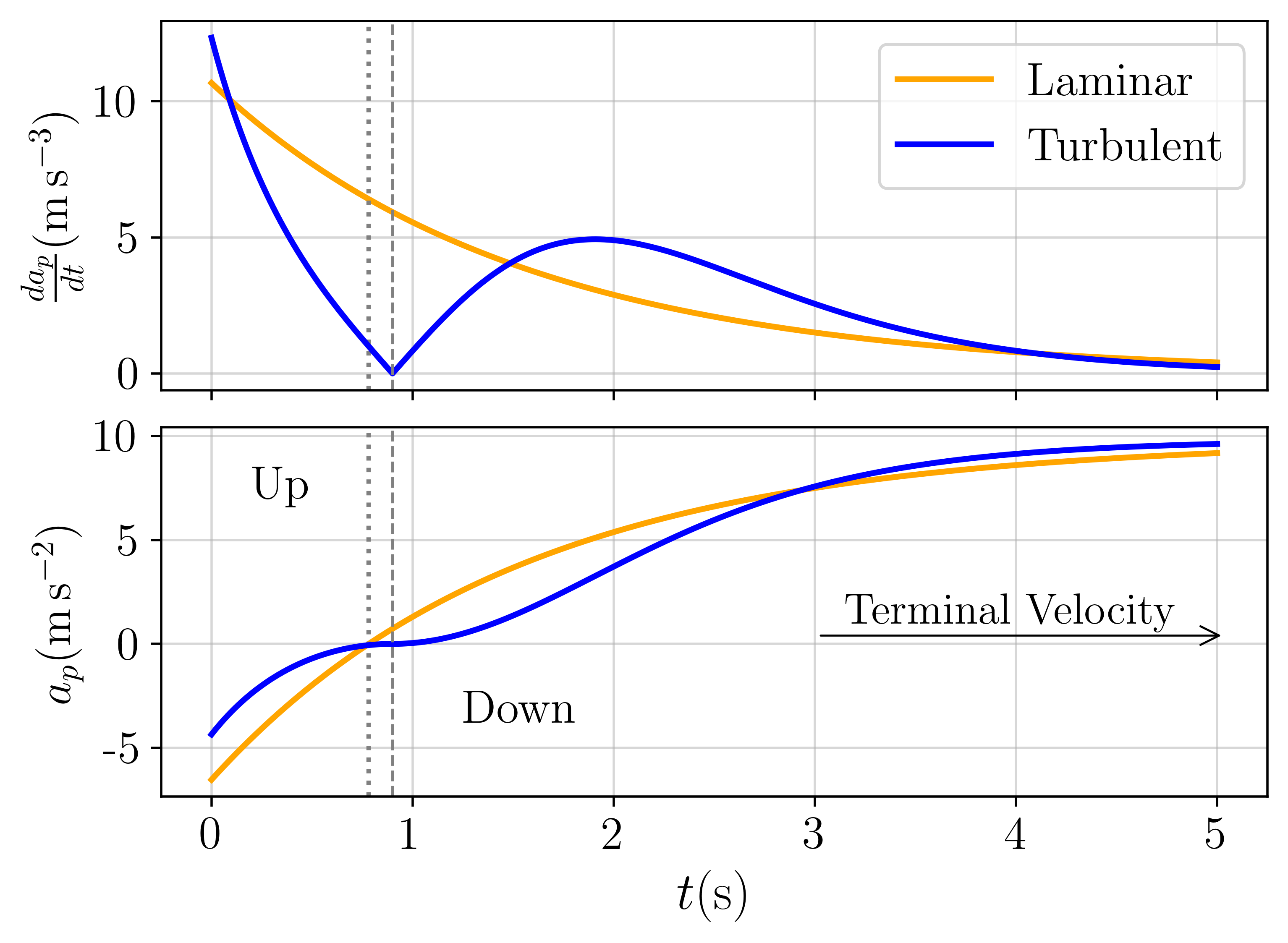
Figure 1: Proper acceleration $a_{p}(t)$ (bottom panel) and its derivative $\frac{da_{p}}{dt}$ (top panel) for laminar (orange line) and turbulent (blue line) flows. Gray vertical lines indicate the apex time for laminar flow ($t_{\text{apex}}=0.78\,\text{s}$, dotted line) and for turbulent flow ($t_{\text{apex}}=0.90\,\text{s}$, dashed line).

A key distinguishing feature between the two flow regimes is the behavior of the proper acceleration curve at the apex. In laminar flow, the curve maintains a consistent concavity throughout the motion, exhibiting simpler behavior. In contrast, turbulent flow introduces more pronounced changes, including an inversion of concavity at the apex. This inversion corresponds to a temporary plateau in the proper acceleration curve near the apex, a consequence of the velocity-squared dependence of drag in turbulent flow. As a result, the object spends more time with near-zero proper acceleration, reflecting a smoother transition between the upward and downward phases of motion.

The proper acceleration curve in the turbulent regime exhibits three distinct regions of concavity throughout the object’s motion. During the upward motion, the concavity is negative. At the apex, it inverts to positive, marking the transition to the downward phase. As the object approaches terminal velocity (approximately two seconds into the fall, as indicated in Fig. 1), the concavity becomes negative again, signaling the final stage of motion.

The top plot of Fig. 1 shows the derivative of the proper acceleration, a quantity known as jerk [9], given by:

$$\frac{da_{p}}{dt}=-(n+1)g\frac{|v|^{n}}{v_{t}^{n+1}}a,$$ (15)

where $a$ is the total acceleration of the object in the Earth’s frame, accounting for both gravity and drag effects, as described by Eq. (7). The negative sign in front of the right-hand side, combined with the fact that the total acceleration $a$ is negative in our reference frame (directed downward), ensures that the derivative of the proper acceleration is always positive. As the object approaches terminal velocity, its proper acceleration converges to $g$. Consequently, its derivative approaches zero, indicating that the system is reaching a steady state, where the drag force approaches a constant value.

In the laminar regime, the derivative of the proper acceleration remains non-zero at the apex. This occurs because the term involving the velocity in the derivative equation is constant, as $|v|^{n}=1$ for $n=0$. To further understand the behavior around the apex, we can examine the second derivative of the proper acceleration, a quantity known as snap [9], evaluated at this point:

$$\left.\frac{d^{2}a_{p}}{dt^{2}}\right|_{t_{\text{apex}}}=-\frac{g^{3}}{v_{t}^{2}}.$$ (16)

This constant, negative value for the second derivative indicates a smooth and continuous decrease in the proper acceleration derivative around the apex in the laminar regime.

In contrast, in the turbulent regime, the derivative of the proper acceleration at the apex is zero because it depends directly on the velocity, which also vanishes at that point. However, due to the dependence on the absolute value of the velocity, the second derivative of the proper acceleration becomes discontinuous at the apex. Specifically, we have:

$$\left.\frac{d^{2}a_{p}}{dt^{2}}\right|_{t_{\text{apex}}}=-2\,\frac{g^{3}}{v_{t}^{2}}\,\text{sign}(v),$$ (17)

where $\text{sign}(v)$ indicates the direction of the velocity. This result shows that the second derivative is negative when approaching from the upward motion (where $v>0$) and positive when coming from the downward motion (where $v<0$), thus defining an inflection point at the apex. Additionally, the magnitude of the second derivative in the turbulent regime is twice that of the laminar regime, highlighting the sharper transition in turbulent flow. Note that this sharper transition in the second derivative contrasts with the smoother overall behavior of the proper acceleration near the apex, as illustrated in Fig. 1.

To emphasize their significance, we reiterate the distinct characteristics of proper acceleration at the apex within the turbulent regime:

1. Proper acceleration reaches zero at the apex, $a_{p}(t_{\text{apex}})=0$.

2. The first derivative of proper acceleration, $\frac{da_{p}}{dt}$, is also zero.

3. The second derivative of proper acceleration, $\frac{d^{2}a_{p}}{dt^{2}}$, is discontinuous and changes sign, indicating an inflection point between the upward and downward phases.

These features highlight the apex as a pivotal point in the analysis of turbulent motion, providing robust criteria for unambiguously identifying the flow regime from acceleration data.

The top plot of Fig. 2 demonstrates the impact of different initial conditions on the proper acceleration in the turbulent drag model. It presents proper acceleration curves for varying initial velocities ($v_{0}=0\,\text{m}\,\text{s}^{-1}$, orange line; $v_{0}=4\,\text{m}\,\text{s}^{-1}$, blue line; and $v_{0}=8\,\text{m}\,\text{s}^{-1}$) while keeping the terminal velocity fixed at $v_{t}=15\,\text{m}\,\text{s}^{-1}$.

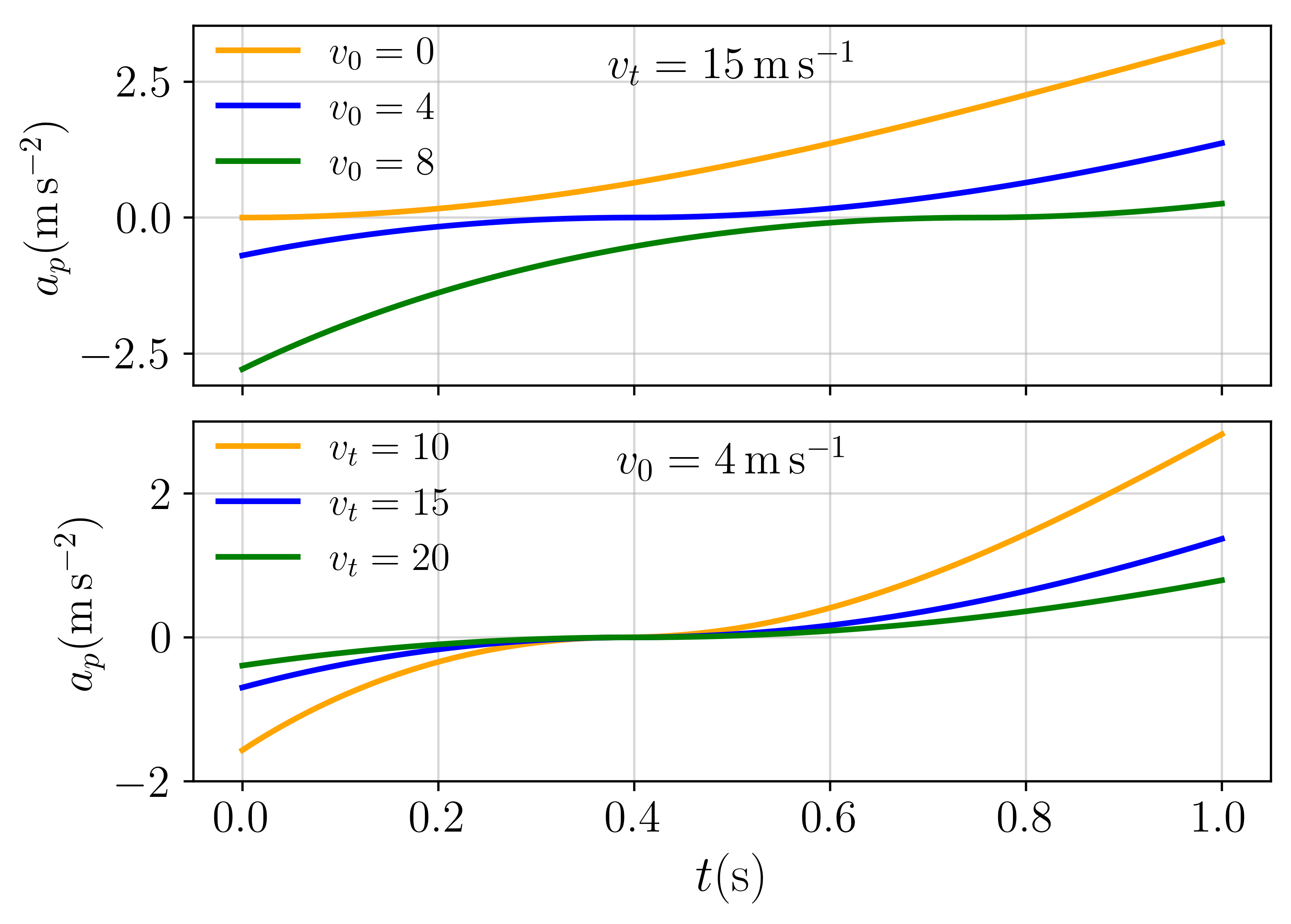
Figure 2: Proper acceleration $a_{p}(t)$ in the turbulent flow regime for varying initial velocities $v_{0}$ (top plot) and terminal velocities $v_{t}$ (bottom plot). In the top plot, the terminal velocity is fixed at $v_{t}=15\,\text{m}\,\text{s}^{-1}$, with initial velocities $v_{0}=0\,\text{m}\,\text{s}^{-1}$ (orange line), $v_{0}=4\,\text{m}\,\text{s}^{-1}$ (blue line), and $v_{0}=8\,\text{m}\,\text{s}^{-1}$ (green line). In the bottom plot, the initial velocity is fixed at $v_{0}=4\,\text{m}/\text{s}$, with terminal velocities $v_{t}=10\,\text{m}/\text{s}$ (orange line), $v_{t}=15\,\text{m}\,\text{s}^{-1}$ (blue line), and $v_{t}=20\,\text{m}\,\text{s}^{-1}$ (green line).

Varying $v_{0}$ results in a horizontal shift of the $a_{p}(t)$ curve without changing its overall shape. This horizontal translation corresponds to a temporal shift in the acceleration profile, affecting the timing of key events, such as reaching the apex or approaching terminal velocity. However, the magnitude of the acceleration remains consistent across different initial velocity values.

The bottom plot of Fig. 2 demonstrates the effect of varying terminal velocities ($v_{t}=10\,\text{m}\,\text{s}^{-1}$, orange line; $v_{t}=15\,\text{m}\,\text{s}^{-1}$, blue line; and $v_{t}=20\,\text{m}\,\text{s}^{-1}$) while keeping the initial velocity fixed at $v_{0}=4\,\text{m}\,\text{s}^{-1}$. As $v_{t}$ increases, both the amplitude and the curvature of the $a_{p}$ curve change, highlighting how terminal velocity influences the object’s deceleration and eventual stabilization.

Notably, while the curve’s shape varies, the time to reach the apex is only marginally affected, with a small shift of just 0.015 seconds across the different $v_{t}$ values considered. This behavior can be understood by analyzing the Taylor series expansion of $t_{\text{apex}}$ given by Eq. (12):

$$t_{\text{apex}}=\frac{v_{0}}{g}\left[1-\frac{1}{3}\left(\frac{v_{0}}{v_{t}}\right)^{2}+\mathcal{O}\left(\frac{v_{0}}{v_{t}}\right)^{4}\right].$$ (18)

The leading-order approximation shows no dependency on $v_{t}$. The next term, proportional to $(v_{0}/v_{t})^{2}$, quantifies the small effect of terminal velocity on the apex time when $v_{0}<v_{t}$.

When analyzing only the descent in the turbulent flow, it is still possible to achieve a reasonable fit for the proper acceleration curve. However, both the initial velocity $v_{0}$ and the terminal velocity $v_{t}$ influence the curve in similar ways, introducing a non-negligible correlation between them. This similarity in their effects means that the constraints on these parameters are relatively loose when considering only the downward motion.

However, the inclusion of the upward motion, together with the apex, introduces strong constraints that significantly reduce this correlation. The apex acts as a critical point in the trajectory, where both $v_{0}$ and $v_{t}$ exert complementary but distinguishable influences. This added information effectively “anchors” the model, ensuring that the parameters are better constrained, leading to a more precise and stable determination of both $v_{0}$ and $v_{t}$.

3 Data Acquisition

In this study, we used an Asus ZenFone Max Pro (M2) [10] smartphone to collect acceleration data during its fall. The accelerometer data were accessed and recorded using the phyphox application [11], a free and open-source tool that provides real-time access to various sensor readings. This app allows for the simple export of collected data in multiple formats, making it suitable for detailed analysis.

3.1 Experimental Setup

The experiments were designed with simplicity and replicability in mind, making them accessible with minimal equipment. The smartphone was either dropped or launched from a height of approximately 1 meter, with care taken to keep the screen parallel to the Earth’s surface and to avoid any unintended rotations, aiming to align the phone’s $z_{p}$-axis with the Earth’s $z$-axis.

Two types of experiments were conducted:

• Fall: In this experiment, the smartphone was released with no significant initial velocity. A total of 22 trials were performed under these conditions.

• Up$-$Down: For this experiment, the smartphone was launched upward with an initial positive velocity. Data were collected throughout both the upward and downward motion phases. A total of 16 trials were conducted for this type of experiment.

Although the Up$-$Down experiment inherently includes a Fall phase, the two experiments were conducted separately to account for additional variability in the Up$-$Down setup. This setup is more prone to differences in initial velocity, as well as unintended inclinations and rotations during the launch. In contrast, the Fall setup, with negligible initial velocity and a more controlled release, potentially reduces these sources of variability.

3.2 Accelerometer Precision and Variability

The Asus ZenFone Max Pro (M2) smartphone used in this experiment is equipped with a Bosch BMI160 accelerometer [12], a 6-axis motion sensor. For this experiment, only the linear acceleration data was used to analyze the smartphone’s motion. The acquisition rate was set to 200 Hz, the default setting in the phyphox application, which proved sufficient for capturing the relevant data.

To evaluate the precision of the Bosch BMI160 accelerometer, two types of data collection were performed: Static and Free-Fall. In the Static method, the smartphone was placed stationary on a flat surface. In the Free-Fall method, the smartphone was dropped with its screen oriented perpendicular to the Earth’s surface, $\hat{z}_{p}\cdot\hat{z}=0$, to minimize drag. Note that this orientation differs from that used in the Fall and Up$-$Down experiments, where $\hat{z}_{p}\cdot\hat{z}=1$. In both methods, the focus was on collecting acceleration data along the $z_{p}$-axis.

For the Static test, 1736 data points were collected over 8.75 seconds. The acceleration along the $z_{p}$-axis was measured as $a_{p}=(9.715\pm 0.022)\,\text{m}\,\text{s}^{-2}$, aligning closely with the expected gravitational acceleration, though indicating a slight tilt relative to the vertical direction. The low variability in the measurements demonstrates the consistency of the accelerometer when stationary. These results align with previous studies, which reported standard deviations ranging from $0.018$ to $0.020\,\text{m}\,\text{s}^{-2}$ using smartphone accelerometers in similar setups [13].

For the Free-Fall tests, three trials were conducted, with the collected data summarized as follows:

• Trial 1: 79 data points collected over 0.39 seconds, with an acceleration of $a_{p}=(-0.250\pm 0.022)\,\text{m}\,\text{s}^{-2}$.

• Trial 2: 95 data points recorded over 0.47 seconds, yielding an acceleration of $a_{p}=(-0.238\pm 0.021)\,\text{m}\,\text{s}^{-2}$.

• Trial 3: 104 data points obtained over 0.52 seconds, with an acceleration of $a_{p}=(-0.244\pm 0.023)\,\text{m}\,\text{s}^{-2}$.

Two important observations emerge from these results. The first is that the standard deviation is similar across all three trials and aligns with the value obtained in the Static test. This indicates that the accelerometer behaves similarly under both stationary and dynamic conditions. The second observation is that the acceleration values show close agreement across the trials, suggesting an intrinsic bias in the measurements, around $-0.240\,\text{m}\,\text{s}^{-2}$. This bias aligns with the zero-g offsets commonly observed in smartphone accelerometers, which can vary significantly between devices [14].

Fig. 3 shows the variability in the accelerometer readings from both the Static and Free-Fall experiments. For both setups, the mean acceleration was subtracted to focus only on the fluctuations. In the Free-Fall setup, the results from three trials were combined into a single dataset. Both distributions—Static (blue) and Free-Fall (orange)—show similar variabilities. A standard deviation of $\sigma_{a_{p}}=0.022\,\text{m}\,\text{s}^{-2}$ was determined for the accelerometer, as indicated by the Gaussian curve (dashed green). This value will be used as the error in the accelerometer measurements for the following data analysis.

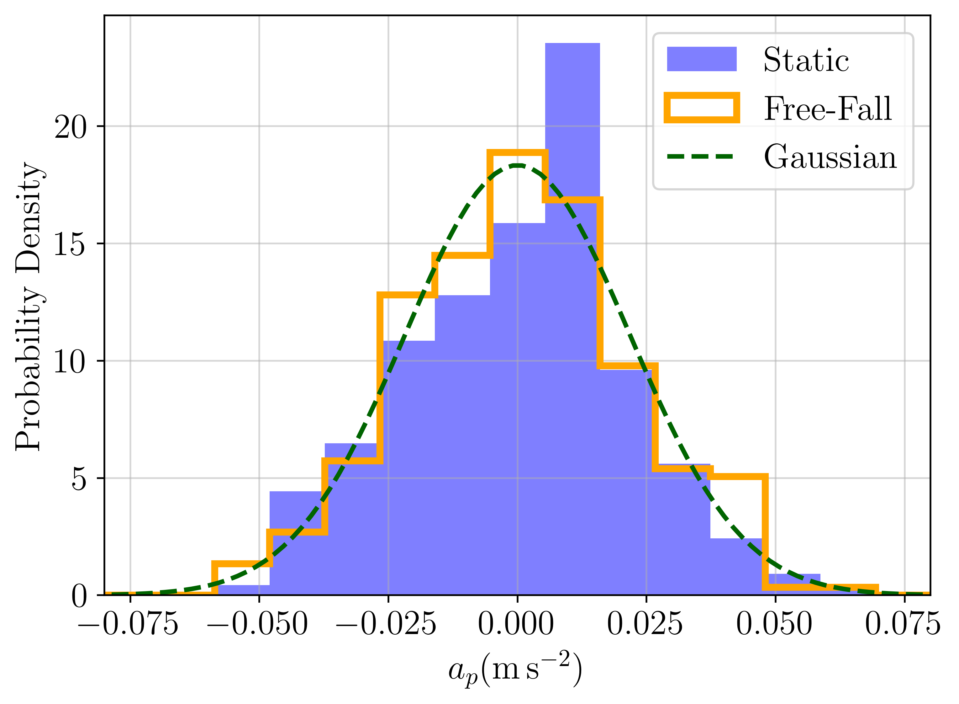
Figure 3: Probability density of proper acceleration $a_{p}$ for both the Static (blue) and Free-Fall (orange) experiments, with their means subtracted. A Gaussian distribution with a standard deviation of $0.022\,\text{m}\,\text{s}^{-2}$ (dashed green) is also shown, reflecting the variability of the accelerometer across both experimental conditions.

3.3 Overview of Collected Data

Before analyzing all 38 datasets from the Fall (22 trials) and Up$-$Down (16 trials) experiments, we begin by focusing on a single Up$-$Down experiment. This initial analysis provides insight into both the upward and downward phases, since the Up$-$Down experiment inherently includes a Fall phase at its end.

Fig. 4 shows the acceleration data recorded by the smartphone’s accelerometer during a typical Up$-$Down experiment. The upper plot presents the raw, unfiltered data along the $z_{p}$-axis, starting just before the smartphone is released and continuing until it impacts the surface. The upward launch is not instantaneous: it begins at 0.8 seconds, when the phone is released, and lasts until around 0.9 seconds, when the accelerometer readings stabilize. The impact is registered by a sharp peak in acceleration just after 1.8 seconds.

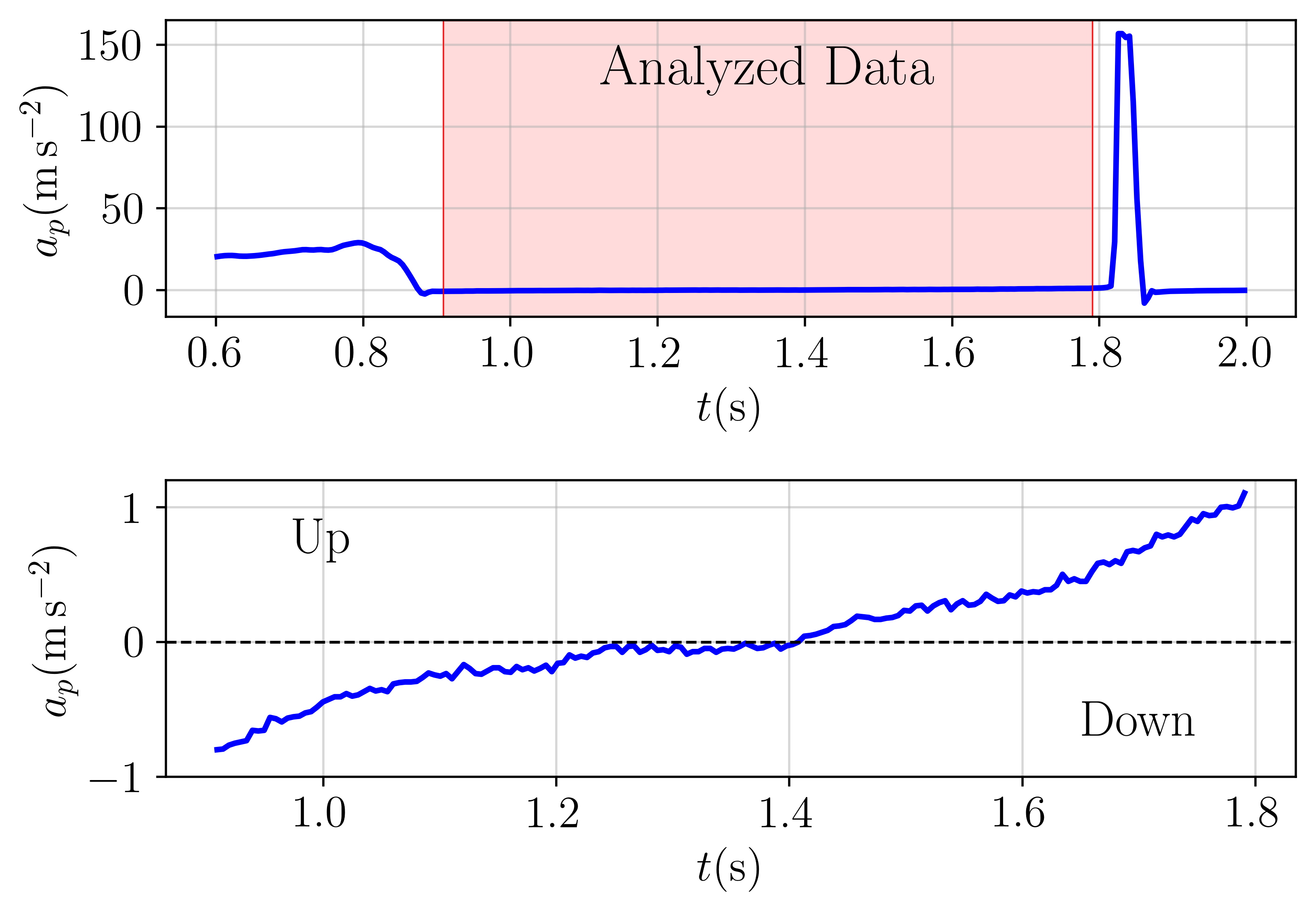
Figure 4: Raw acceleration data recorded by the smartphone’s accelerometer ($z_{p}$ component) during a trial of the Up$-$Down experiment. The upper plot shows the unfiltered data from just before the smartphone’s release until its impact with the surface, with the shaded red region marking the interval selected for detailed analysis. The lower plot provides a zoomed-in view of this interval, with “Up” and “Down” annotations indicating the upward and downward phases as the smartphone transitions between them.

The red-highlighted section in the upper plot of Fig. 4 marks the period during which the smartphone is influenced only by gravity and air resistance, from release to impact. This data was selected through visual inspection, carefully excluding any residual effects from the release and the impact. As the smartphone approaches the surface, changes in the accelerometer data may occur due to additional forces. One possible source is the ground effect (or air cushion effect), where the compressed air beneath the smartphone creates a lift force that can become significant compared to the drag force [15]. To maintain focus on the drag force during the fall, we excluded data points near impact to minimize these effects.

A closer look at the analyzed data region, shown in the bottom plot of Fig. 4, offers a more detailed view. Visual inspection reveals that the laminar flow model fails to capture the observed behavior. Specifically, the data shows a transition at the apex, marked by a change in the concavity of the acceleration curve—an effect not captured by this model (see Fig. 1). In the downward phase, corresponding to a Fall experiment, the concavity of the curve is also inverted compared to what the laminar model would suggest. These discrepancies confirm that this model is inadequate for describing the smartphone’s accelerometer readings. Therefore, our subsequent analysis will focus exclusively on the turbulent model, which provides a better fit to the data.

To corroborate our focus on the turbulent model, we estimate the Reynolds number (Re) [4] for the falling smartphone:

$$\text{Re}=\frac{\rho vL}{\mu}.$$ (19)

where $\rho=1.184\,\text{kg}\,\text{m}^{-3}$ is the air density and $\mu=1.849\times 10^{-5}\,\text{kg}\,\text{m}^{-1}\,\text{s}^{-1}$ is the air dynamic viscosity, both at $25\,^{\circ}\text{C}$ and 1 atm [16]. For a typical smartphone and drop, we have $L=0.1\,\text{m}$ and $v=10\,\text{m}\,\text{s}^{-1}$. Substituting these values yields $\text{Re}\approx 6.4\times 10^{4}$. This result is well above the critical Reynolds number for flow transition, around $\text{Re}\approx 3000$ [4], indicating that the flow around the falling smartphone is likely turbulent, supporting our choice of the turbulent model for analysis.

We now expand our analysis to the full set of acceleration measurements from both experiments. By analyzing the 22 Fall and 16 Up$-$Down trials, we aim to capture the variability across them and gain a more comprehensive understanding of the smartphone’s motion under varying experimental conditions.

In Fig. 5, the measured proper acceleration ($a_{p}$) is displayed for all experiments, with the Fall data in the left plot and the Up$-$Down data in the right plot. In both plots, thin red lines represent individual measurements, while the blue line shows the mean acceleration across the dataset. The shaded blue region around the blue line corresponds to the standard deviation, providing insight into the variability between measurements. For the Fall experiment, the average duration was 0.53 seconds (ranging from 0.44 to 0.60), while for the Up$-$Down experiment, it was longer, averaging 0.84 seconds (ranging from 0.76 to 0.89).

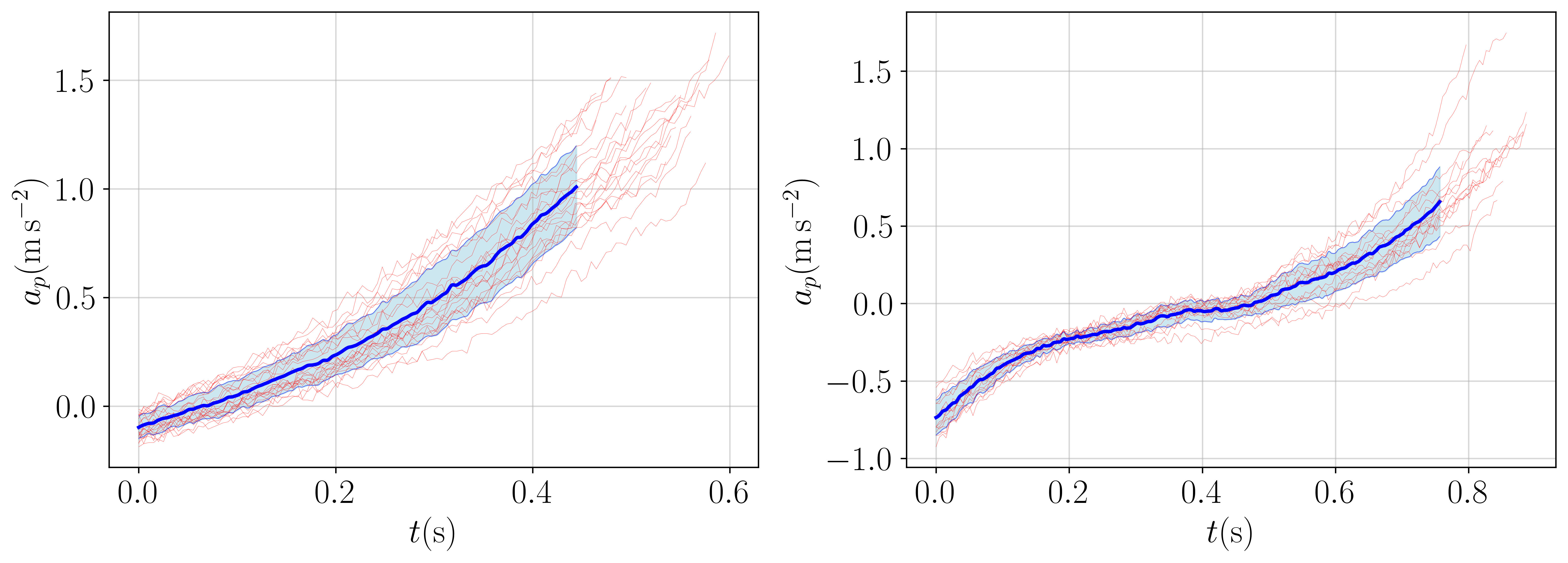
Figure 5: Proper acceleration ($a_{p}$) measured during the Fall (left) and Up$-$Down (right) experiments. Thin red lines represent individual measurements, while the blue line indicates the mean across the dataset. The shaded blue region corresponds to the standard deviation, offering a measure of variability between experiments.

To compute the mean acceleration and its standard deviation (represented by the blue line and the shaded blue region in Fig. 5), we applied interpolation to the data from each trial using an Akima spline [17]. This method was selected for its ability to minimize overshoot, ensuring smooth interpolation while preserving the integrity of the original data. Interpolation was necessary due to slight variations in both the motion duration and the specific time points of recorded measurements. By aligning the data points consistently across trials, we obtained a more reliable mean and standard deviation. The analysis was restricted to the minimum motion duration observed (0.44 seconds for the Fall experiments and 0.76 seconds for the Up$-$Down), ensuring that only data within the shared time window were included.

The interpolated data sets, from which the mean and standard deviation were obtained, are referred to as the Grouped Data in the subsequent analysis, with separate sets created for both the Fall and Up$-$Down experiments. These data sets were constructed using an acquisition rate of 200 Hz, consistent with the rate used in the experiments. The use of Grouped Data provides a standardized framework for comparing trials, offering insights into the variability of factors such as initial velocity, tilt, and rotation of the smartphone. In complementing the 38 individual experimental trials, the Grouped Data helps explore how variations in the experimental setup influence the results. While not intended for rigorous scientific analysis, this approach serves as a valuable pedagogical tool.

The variability observed in the Grouped Data can now be compared with the intrinsic variability of the accelerometer, determined as $\sigma_{a_{p}}=0.022\,\text{m}\,\text{s}^{-2}$ (as defined in Section 3.2). For the Fall experiment, the standard deviation of the Grouped Data ranged from $0.046\,\text{m}\,\text{s}^{-2}$ to $0.195\,\text{m}\,\text{s}^{-2}$. Similarly, for the Up$-$Down experiment, the standard deviation showed values between $0.031\,\text{m}\,\text{s}^{-2}$ and $0.225\,\text{m}\,\text{s}^{-2}$. These values are notably larger than the intrinsic variability of the accelerometer, reflecting additional sources of variation inherent to the experimental setup, such as differences in initial velocity, tilt, and rotation across trials.

A noteworthy pattern in the data is the reduction in variability when the smartphone’s velocity is near zero. In the Fall experiment, this occurs at the start of the motion, while in the Up$-$Down experiment, it takes place around the apex of the trajectory. Fig. 5 clearly shows this behavior, with the shaded region representing the standard deviation narrowing significantly during these phases. For the Fall experiment, the reduced variability at the start is expected, given our efforts to initiate the motion with zero initial velocity. In the Up$-$Down experiment, the consistency near the apex suggests regularity in the motion during this phase, despite differences in the initial launch conditions, as anticipated in Section 2.3.

Interestingly, the variability observed between trials in both experiments is comparable, despite the Fall experiment being designed to minimize it. This suggests that factors such as initial conditions, tilt, or rotation still introduced significant fluctuations, limiting the intended goal in reducing trial-to-trial variability in the Fall set up.

Additionally, a consistent bias of approximately $-0.1\,\text{m}\,\text{s}^{-2}$ was observed in both experiments. In the Fall experiment, this bias is most noticeable at the beginning of the motion, whereas in the Up$-$Down experiment, it becomes more evident near the apex of the trajectory. Although this value is slightly smaller than the bias reported in Section 3.2, it remains consistent with the overall trend identified in the accelerometer measurements.

In the subsequent analysis, the intrinsic error of the accelerometer will be used for individual trial fits, while the Grouped Data will employ the standard deviation across datasets to account for the variability observed between experiments.

4 Data Analysis

In this section, we present the analysis of the acceleration data collected from the smartphone during both the Fall and Up$-$Down experiments (see Section 3.1). The smartphone’s embedded accelerometer recorded proper acceleration (the acceleration measured in the phone’s reference frame) as a function of time. The analysis focuses on both individual trials and their Grouped Data (see Section 3.3), applying the turbulent drag model discussed in Section 2.2.

4.1 Methodology for Model Fitting

To fit the turbulent drag model to the experimental data, we employed the Weighted Least Squares (WLS) method, where the weights are given by the inverse square of the corresponding uncertainties [18]. In this approach, the goal is to minimize the weighted sum of the squared residuals, denoted by $\varepsilon_{i}$. The residuals are defined as the difference between the observed data points, $a_{p}(t_{i})$, and the corresponding values predicted by the model at each measured time, $\hat{a}_{p}(t_{i};\vec{\theta})$:

$$\varepsilon_{i}=a_{p}(t_{i})-\hat{a}_{p}(t_{i};\vec{\theta}).$$ (20)

The free parameters of the model are encapsulated in $\vec{\theta}$.

Our model, developed in Section 2, requires an additional free parameter to fully describe the data: the bias inherent in the accelerometer readings. This bias is evident in Figs. 4 and 5, and was also observed when assessing its variability in Section 3.2. To account for this effect, we introduce an offset, $\Delta a$, to our proper acceleration model (see Eq. 8):

$$\hat{a}_{p}=a_{p}+\Delta a.$$ (21)

The model $\hat{a}_{p}$, now fully defined, includes the gravitational acceleration $g$, the initial velocity $v_{0}$, the terminal velocity $v_{t}$, and the offset $\Delta a$ to account for the accelerometer bias.

The proper acceleration given by Eqs. 8, 11, 12, and 14 shows that the gravitational acceleration $g$ and the terminal velocity $v_{t}$ always appear as ratios: $g/v_{t}$ or $g/v_{t}^{2}$. This reveals a degeneracy in the model, as changes in $g$ can be compensated by corresponding changes in $v_{t}$, making it difficult to independently determine both parameters from the data. In practical terms, this means that the fitting process may yield multiple combinations of $g$ and $v_{t}$ that produce similar results, leading to ambiguity in the interpretation of the model parameters.

To address this issue, we fixed the value of $g$ at $9.8\,\text{m}\,\text{s}^{-2}$, consistent with the gravitational acceleration near the Earth’s surface. This choice eliminates the degeneracy, allowing us to focus on accurately estimating $v_{t}$, the parameter directly related to air resistance affecting the smartphone’s motion. As a result, our model now includes three free parameters:

$$\vec{\theta}=(v_{0},v_{t},\Delta a).$$ (22)

These three parameters will be estimated in the subsequent analysis for both the Fall and Up$-$Down experiments.

4.2 Fall Results

We begin by presenting the fitting results for the 22 individual trials from the Fall experiment. Each trial provided three fitted parameters: the initial velocity $v_{0}$, the terminal velocity $v_{t}$, and the offset $\Delta a$. In total, 66 parameters were obtained across all trials.

The fit of the turbulent drag model to a single dataset from the Fall experiment is shown in Fig. 6. This particular trial was selected because its reduced chi-square value, $\chi^{2}/\text{dof}=1.77$, is close to the average value across all 22 trials, making it representative of the overall dataset. Although the terminal velocity, $v_{t}=(17.29\pm 0.27)\,\text{m}\,\text{s}^{-1}$, is the highest among all experiments, the model fits the data well, achieving a coefficient of determination $R^{2}=0.9938$. The fitted initial velocity was $v_{0}=(-1.29\pm 0.13)\,\text{m}\,\text{s}^{-1}$, indicating that the smartphone was already moving downward when data collection began. The offset was $\Delta a=(-0.16\pm 0.02)\,\text{m}\,\text{s}^{-2}$, reflecting the expected negative bias in the accelerometer readings.

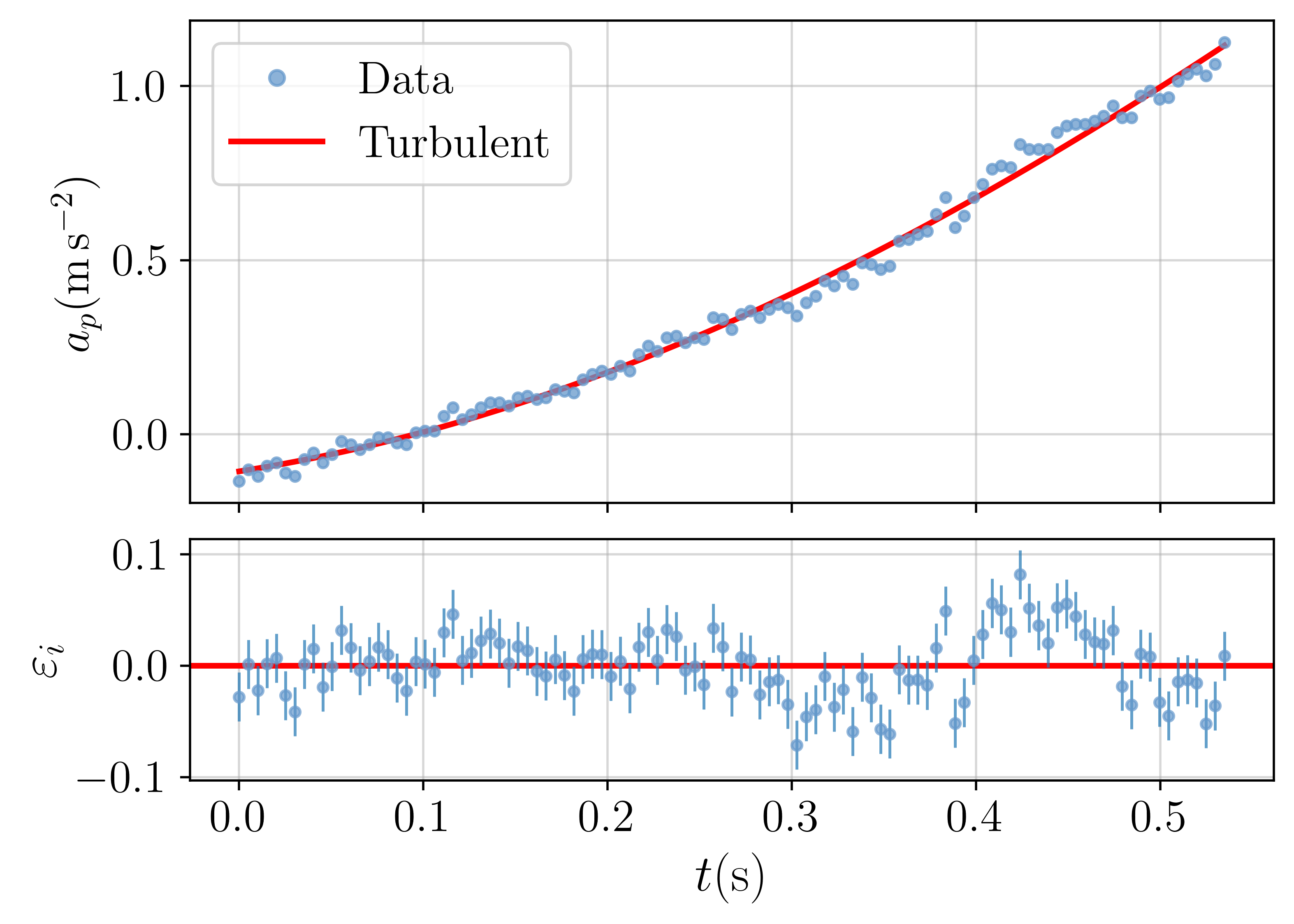
Figure 6: Fit of the turbulent drag model to a single dataset from the Fall experiment. The top plot displays the proper acceleration $a_{p}$ as a function of time, showing experimental data (blue points) and the model fit (red line). The bottom plot illustrates the residuals $\varepsilon_{i}$. Error bars indicate the uncertainty in the accelerometer measurements, $\sigma_{a_{p}}=0.022\,\text{m}\,\text{s}^{-2}$. Further details of this fit are provided in the main text.

The uncertainties in the fitted parameters, derived from the WLS method, exhibited significant variation across all 22 trials. For the initial velocity $v_{0}$, the uncertainties ranged from $0.044\,\text{m}\,\text{s}^{-1}$ to $0.193\,\text{m}\,\text{s}^{-1}$, and for the terminal velocity $v_{t}$, from $0.096\,\text{m}\,\text{s}^{-1}$ to $0.348\,\text{m}\,\text{s}^{-1}$. The offset in the proper acceleration, $\Delta a$, which accounts for the accelerometer bias, had uncertainties between $0.006\,\text{m}\,\text{s}^{-2}$ and $0.027\,\text{m}\,\text{s}^{-2}$. These relatively large ranges of uncertainty result from the correlation between the initial and terminal velocities in the Fall experiment. Since no data are available from the upward motion (and thus no information from the apex), the ability to constrain the model is limited, as discussed in Section 2.3. Notably, the three trials with positive initial velocities, although small (with the highest being just $0.14\,\text{m}\,\text{s}^{-1}$), yielded significantly smaller parameter errors. This suggests that even slight upward motion provides additional information, improving the model’s constraints.

The results of the 22 trials, when considered collectively, are summarized in Table 1. The values presented correspond to the mean and standard deviation across all experiments, rather than the uncertainties derived from the WLS method. The coefficient of determination, $R^{2}$, shows consistently high values, with $0.9951\pm 0.0020$, indicating good agreement between the experimental data and the turbulent drag model. The reduced chi-square, $\chi^{2}/\text{dof}=1.76\pm 0.49$, reflects an overall good fit, further supporting the robustness of the model despite some variability between trials.

Parameter	Individual Trials	Grouped Data
$R^{2}$	$0.9951\pm 0.0020$	$0.9984$
$\chi^{2}/\text{dof}$	$1.76\pm 0.49$	$0.011$
$v_{0}\,(\text{m}\,\text{s}^{-1})$	$-0.78\pm 0.64$	$-1.24\pm 0.63$
$v_{t}\,(\text{m}\,\text{s}^{-1})$	$14.74\pm 1.37$	$15.91\pm 1.62$
$\Delta a\,(\text{m}\,\text{s}^{-2})$	$-0.11\pm 0.06$	$-0.14\pm 0.07$

Table 1: Summary of the results from the Fall Experiment. The parameters include the coefficient of determination ($R^{2}$), the reduced chi-square ($\chi^{2}/\text{dof}$), initial velocity ($v_{0}$), terminal velocity ($v_{t}$), and the offset ($\Delta a$). The Individual Trials column displays the mean and standard deviation between the individual experiments, while the Grouped Data column shows the results obtained by analyzing the entire dataset collectively. The uncertainties in the Grouped Data were derived using the Weighted Least Squares (WLS) method.

Regarding the fitted parameters, the initial velocity $v_{0}=(-0.78\pm 0.64)\,\text{m}\,\text{s}^{-1}$ shows considerable variability. This spread may be partly attributed to the experimental setup but is more likely due to the process of selecting the starting point for data collection, which could introduce variability in the determination of the initial velocity. Notably, in all but three trials, the initial velocity was negative, indicating that the smartphone had already started moving downward when data collection began. The terminal velocity $v_{t}=(14.74\pm 1.37)\,\text{m}\,\text{s}^{-1}$ also exhibited a notable spread, with approximately 10% variation between trials.

The offset in the proper acceleration, $\Delta a=(-0.11\pm 0.06)\,\text{m}\,\text{s}^{-2}$, exhibited a consistent trend, with only two trials yielding slightly positive values close to zero. This pattern confirms that the accelerometer’s bias was generally shifted toward negative values. Such small, stable offsets align with the expected behavior of the sensor, as discussed in Section 3.2.

We also analyzed the Grouped Data, with the results shown in the third column of Table 1 and illustrated in Fig. 7. The high $R^{2}$ value $(0.9984)$ indicates good agreement with the model, while the low $\chi^{2}/\text{dof}=0.011$ reflects the larger error bars used to capture the variability across trials. Additionally, the Grouped Data shows a slightly lower initial velocity $(-1.24\pm 0.63)\,\text{m}\,\text{s}^{-1}$ and a higher terminal velocity $(15.91\pm 1.62)\,\text{m}\,\text{s}^{-1}$ compared to the individual trials, suggesting a tendency toward faster falls in the aggregated data. These results align closely with those obtained from individual trials, offering a unified perspective of the experiment.

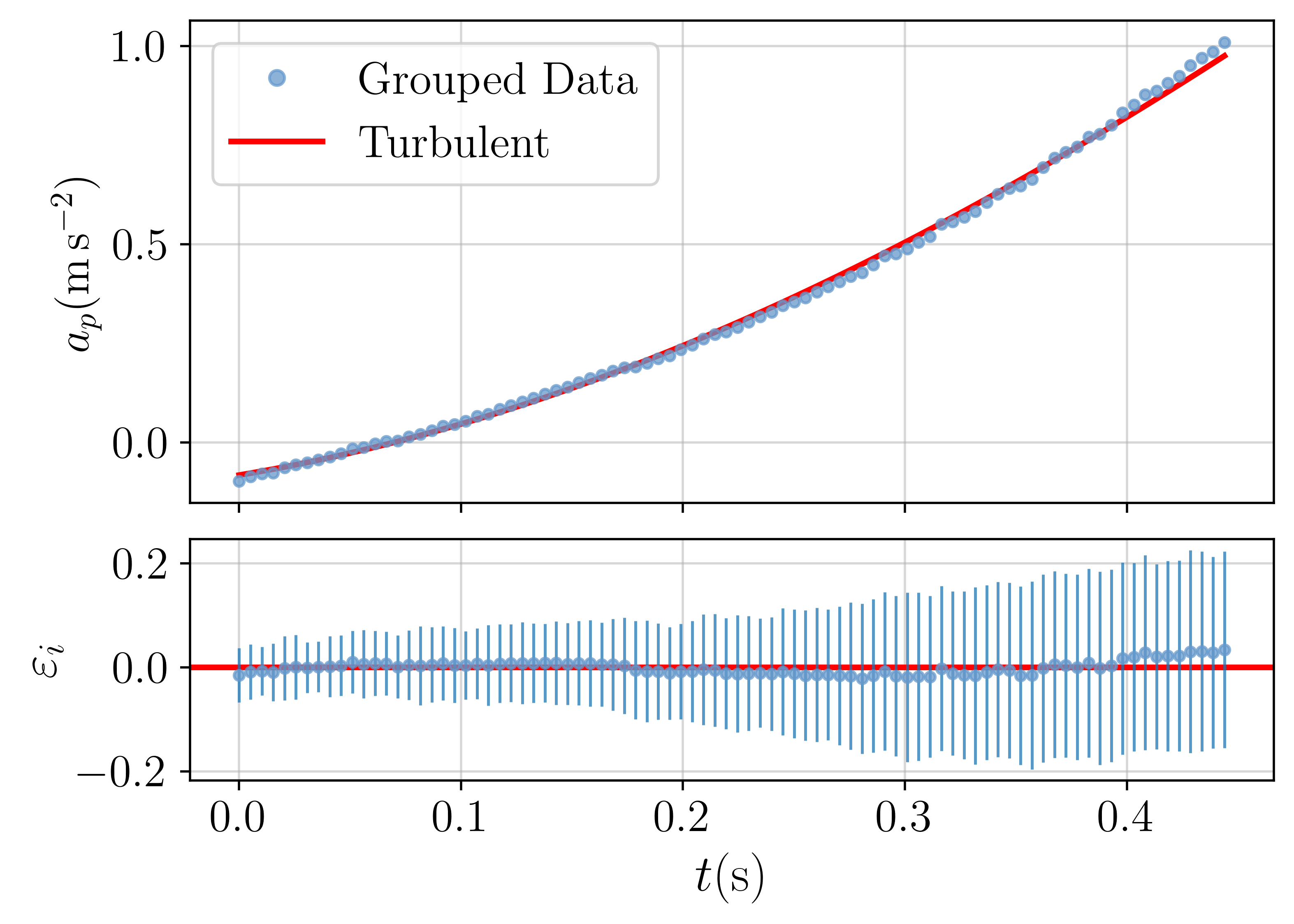
Figure 7: Fit of the turbulent drag model to the Grouped Data from the Fall experiment. The top plot shows the proper acceleration $a_{p}$ as a function of time, with experimental data (blue points) and the model fit (red line). The bottom plot presents the residuals $\varepsilon_{i}$, with error bars capturing the variability across the 22 trials, as described in Section 3.3. The detailed results of this fit are provided in the main text.

These results demonstrate that the turbulent drag model provides a reasonable description of the smartphone’s motion, despite the variability introduced by the experimental setup. While uncertainties in individual trials are present, the model offers a consistent framework for analyzing the dynamics of the fall.

4.3 Up-Down Results

The fitting results of the turbulent drag model for a single dataset from the Up$-$Down experiment are shown in Fig. 8. This trial was selected because its chi-square value, $\chi^{2}/\text{dof}=5.08$, is close to the average across all trials. The relatively high chi-square value may result from tilt and rotations during the Up$-$Down experiment, which are not accounted for in the model. Nonetheless, the model aligns well with the experimental data, achieving a coefficient of determination $R^{2}=0.9874$. The fitted initial velocity was $v_{0}=(3.21\pm 0.02)\,\text{m}\,\text{s}^{-1}$, indicating upward motion at release. The terminal velocity was $v_{t}=(13.34\pm 0.03)\,\text{m}\,\text{s}^{-1}$, and the offset in the proper acceleration was $\Delta a=(-0.07\pm 0.004)\,\text{m}\,\text{s}^{-2}$.

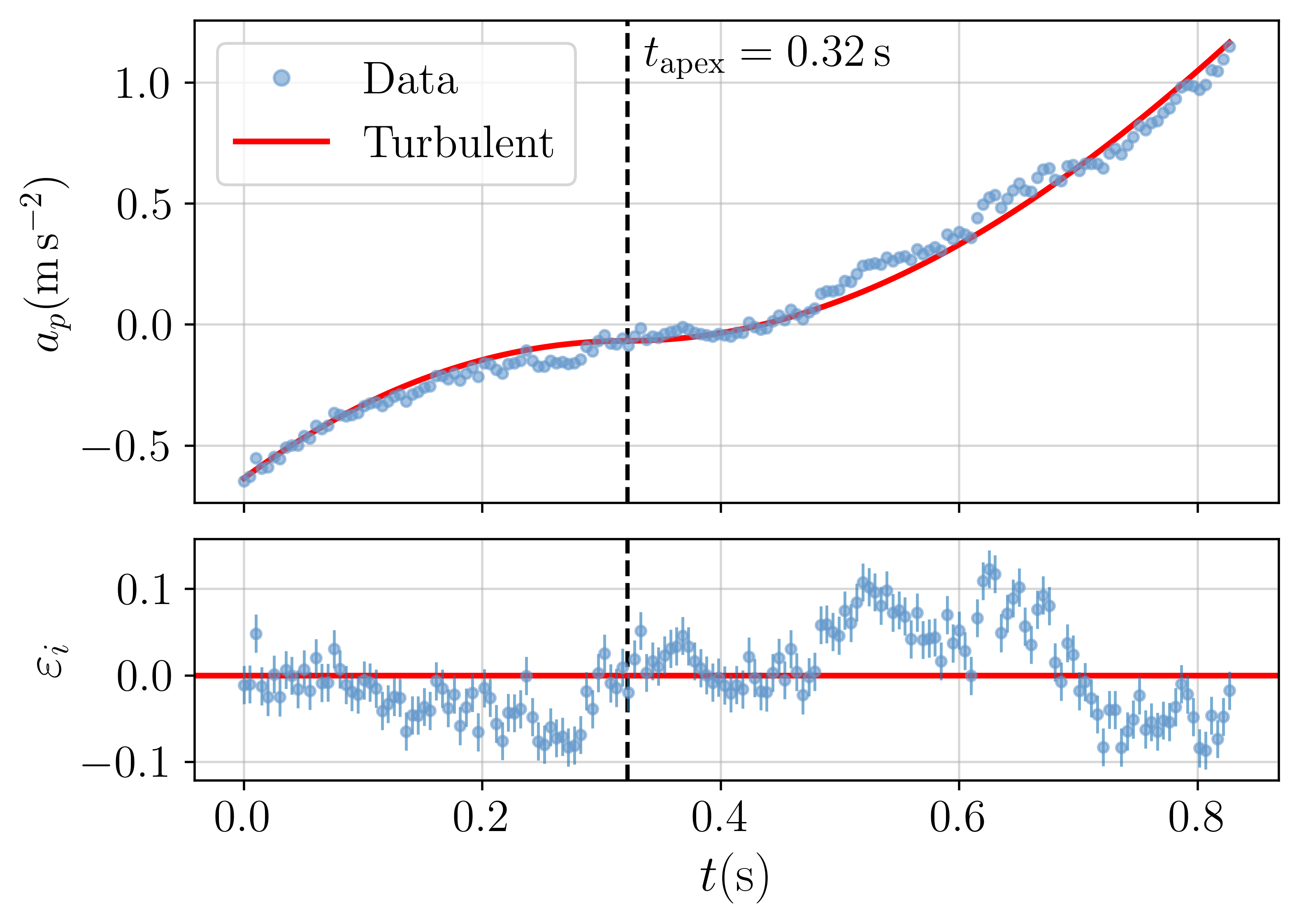
Figure 8: Fit of the turbulent drag model to a single dataset from the Up$-$Down experiment. The top plot shows the proper acceleration $a_{p}$ as a function of time, with experimental data (blue points) and the model fit (red line). The dashed vertical line indicates the time $t_{\text{apex}}$, marking the transition from upward to downward motion. The bottom plot presents the residuals $\varepsilon_{i}$. The error bars represent the uncertainty in the accelerometer measurements, $\sigma_{a_{p}}=0.022\,\text{m}\,\text{s}^{-2}$. The detailed results of this fit are discussed in the main text.

The uncertainties in the fitted parameters, derived from the WLS method, exhibited both minimal variation and small absolute values across the 16 individual trials. For the initial velocity $v_{0}$, they ranged from $0.014\,\text{m}\,\text{s}^{-1}$ to $0.021\,\text{m}\,\text{s}^{-1}$, while for the terminal velocity $v_{t}$, the range was $0.025\,\text{m}\,\text{s}^{-1}$ to $0.051\,\text{m}\,\text{s}^{-1}$. The offset in the proper acceleration $\Delta a$ had variations between $0.0034\,\text{m}\,\text{s}^{-2}$ and $0.0037\,\text{m}\,\text{s}^{-2}$, indicating that the model was well constrained.

These small variations and low magnitudes reflect a more precise parameter estimation compared to the Fall experiment, where uncertainties were notably larger. As discussed in Section 2.3, this improved precision in best-fit parameteres for the Up$-$Down trials was expected. The inclusion of data from both the upward and downward motion, particularly the apex, provided additional information, tightening the model constraints.

The results of the 16 individual trials from the Up$-$Down experiment are summarized in the second column of Table 2. The coefficient of determination was $R^{2}=0.9855\pm 0.0049$, which, although slightly lower than that observed in the Fall experiment, still indicates a reasonably good model fit. The reduced chi-square, $\chi^{2}/\text{dof}=5.08\pm 2.79$, was considerably higher, likely due to the strong constraints imposed by the apex, which limit the model’s flexibility.

Parameter	Individual Trials	Grouped Data
$R^{2}$	$0.9855\pm 0.0049$	$0.9934$
$\chi^{2}/\text{dof}$	$5.08\pm 2.79$	$0.152$
$v_{0}\,(\text{m}\,\text{s}^{-1})$	$3.60\pm 0.36$	$3.52\pm 0.07$
$v_{t}\,(\text{m}\,\text{s}^{-1})$	$14.06\pm 1.13$	$13.77\pm 0.22$
$\Delta a\,(\text{m}\,\text{s}^{-2})$	$-0.08\pm 0.06$	$-0.10\pm 0.01$

Table 2: Summary of the results from the Up$-$Down Experiment. The parameters include the coefficient of determination ($R^{2}$), the reduced chi-square ($\chi^{2}/\text{dof}$), initial velocity ($v_{0}$), terminal velocity ($v_{t}$), and the offset ($\Delta a$). The Individual Trials column displays the mean and standard deviation between the individual experiments, while the Grouped Data column shows the results obtained by analyzing the entire dataset collectively. The uncertainties in the Grouped Data were derived using the Weighted Least Squares (WLS) method.

Regarding the fitted parameters, the initial velocity averaged $v_{0}=(3.60\pm 0.36)\,\text{m}\,\text{s}^{-1}$, reflecting the upward motion of the smartphone at release. The small variability in $v_{0}$ across trials suggests a consistent launch between experiments. In contrast, the terminal velocity, $v_{t}=(14.06\pm 1.13)\,\text{m}\,\text{s}^{-1}$, showed greater variability, reflecting its sensitivity to minor changes in experimental conditions. The offset in proper acceleration, $\Delta a=(-0.08\pm 0.06)\,\text{m}\,\text{s}^{-2}$, remained consistently negative across most trials, indicating a slight bias in the accelerometer readings.

The fitting result for the Grouped Data from the Up$-$Down experiment is shown in Fig. 9 and summarized in the third column of Table 2. The coefficient of determination, $R^{2}=0.9934$, indicates a strong agreement between the model and the experimental data. However, the reduced chi-square value, $\chi^{2}/\text{dof}=0.152$, is notably low, likely due to the larger error bars accounting for variability across trials, which result in a smoother fit. The best-fit initial velocity for the Grouped Data was $v_{0}=(3.52\pm 0.07)\,\text{m}\,\text{s}^{-1}$, closely aligning with the results from the individual trials. Similarly, the terminal velocity was $v_{t}=(13.77\pm 0.22)\,\text{m}\,\text{s}^{-1}$, and the offset in the proper acceleration was $\Delta a=(-0.10\pm 0.01)\,\text{m}\,\text{s}^{-2}$. These results provide a comprehensive overview of the average behavior of the smartphone’s motion across all trials, confirming the consistency between individual and Grouped Data.

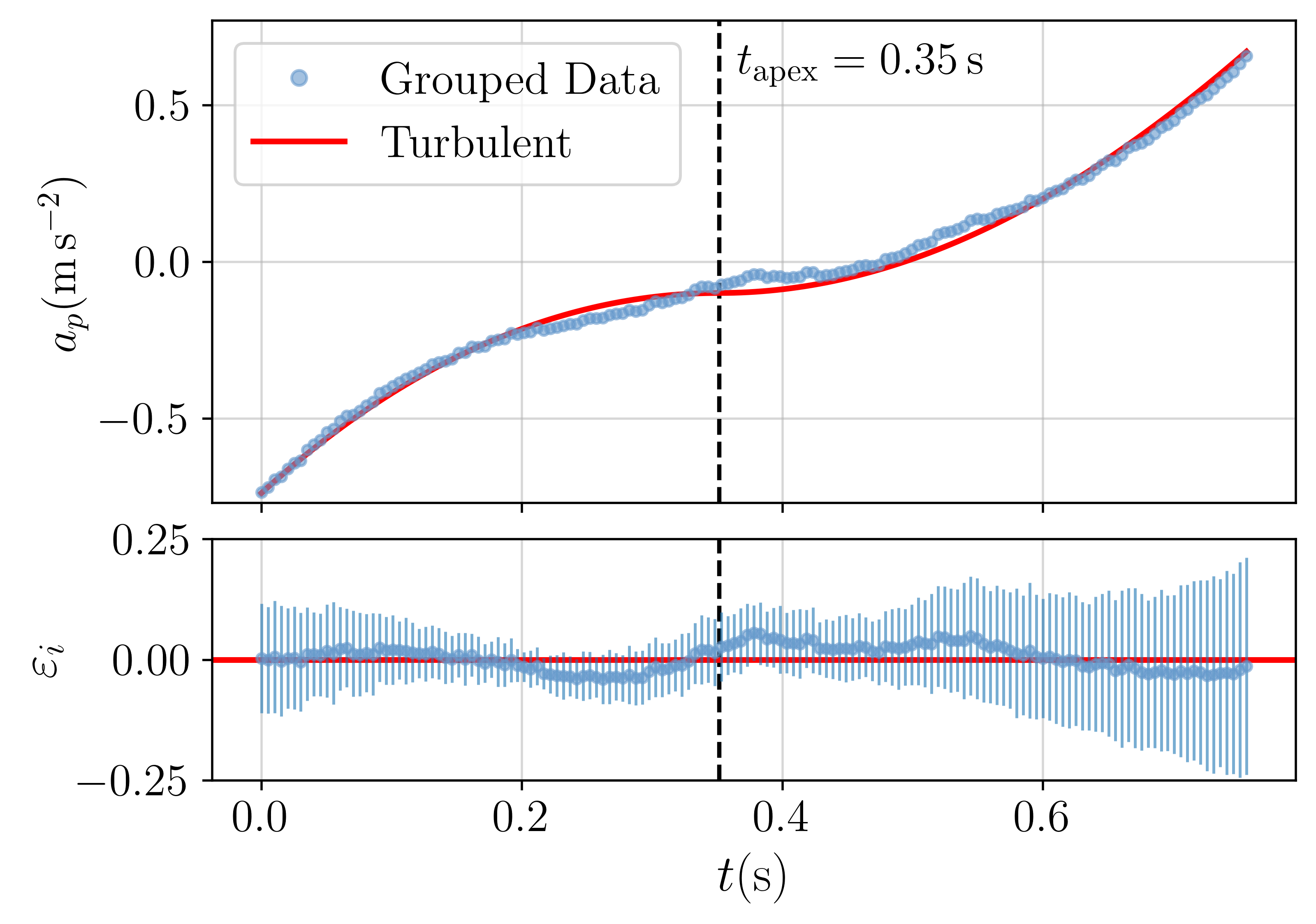
Figure 9: Fit of the turbulent drag model to the Grouped Data from the Up$-$Down experiment. The top plot shows the proper acceleration $a_{p}$ as a function of time, with experimental data (blue points) and the model fit (red line). The bottom plot presents the residuals $\varepsilon_{i}$, with error bars capturing the variability across the 16 trials, as described in Section 3.3. The detailed results of this fit are provided in the main text.

Interestingly, although the best-fit parameters for the individual trials and the Grouped Data are quite similar, the variability across the 16 individual experiments is notably larger than the uncertainties obtained from the WLS method for the Grouped Data. While the Grouped Data exhibits relatively large error bars in $a_{p}$ due to trial-to-trial variability, the strong constraint provided by the apex ensures the model remains well-defined. Additionally, the error near the apex is smaller, further enhancing the model’s constraints in this experiment. This contrasts with the Fall experiment, where both the best-fit parameters and uncertainties between individual trials and Grouped Data were closely aligned, with no significant deviation observed.

These results illustrate the impact of incorporating the upward motion into the analysis, providing tighter constraints on the turbulent drag model. This emphasizes the effectiveness of the Up$-$Down experiment in yielding more precise insights into the dynamics of air resistance. By accounting for both phases of motion and leveraging the constraining power of the apex, the experiment enhances the accuracy of the model’s predictions.

5 Discussions and Conclusions

One notable aspect of this study is the accessibility and simplicity of its experimental setup. By leveraging the smartphone’s built-in accelerometer, this experiment enables the exploration of air drag through a straightforward procedure. The process involves dropping or launching the smartphone vertically, ensuring simple and repeatable data collection. No specialized equipment is required, making the setup practical for various contexts, including classroom environments or independent testing. Additionally, the simplicity of the procedure shifts the focus towards data analysis, offering valuable experience in experimental methods and insights into important aspects of data interpretation.

While the simplicity of the setup is advantageous, it also introduces challenges, particularly in controlling the smartphone’s launch with precision. However, this inherent variability, along with the uncertainties in each trial, provides an opportunity to explore how differences in experimental conditions influence the results. Factors such as variations in initial velocity, tilt, or unintended rotations of the smartphone can affect the acceleration profiles (see Fig. 5). Conducting multiple trials helps identify these effects, emphasizing the importance of repeated measurements and careful consideration of uncertainties during data interpretation.

Despite the inherent variability, the experiment effectively distinguishes between laminar and turbulent drag regimes through the analysis of the proper acceleration data. Laminar flow exhibits a smooth, gradual behavior in the acceleration profile, whereas turbulent flow presents more pronounced characteristics (see Fig. 1). In the turbulent regime, the motion begins with negative concavity during the upward phase, followed by an inflection point at the apex where the concavity becomes positive. As the object approaches terminal velocity in the downward phase, the concavity shifts back to negative. These distinct patterns in the data enable a straightforward differentiation between the two flow regimes.

The experimental data shown in Fig. 5, along with the theoretical models in Fig. 1, indicate that laminar flow does not adequately capture the observed acceleration profiles. Consequently, the analysis focused exclusively on the turbulent model, which more accurately represents the acceleration behavior observed in the experiments.

A total of 22 Fall and 16 Up$-$Down experiments were conducted (see Section 3.1 for details), with the results summarized in Tables 1 and 2, respectively (refer to Sections 4.2 and 4.3). Both tables present the outcomes of individual trials and Grouped Data (as defined in Section 3.3).

The offset results remained consistent across all trials, confirming the negative bias previously identified in the accelerometer measurements (see Section 3.2). As expected, the initial velocity varied according to the different launching conditions: negative to near-zero values in the Fall experiments, $(-0.78\pm 0.64)\,\text{m}\,\text{s}^{-1}$, and positive in the Up$-$Down experiments, $(3.60\pm 0.36)\,\text{m}\,\text{s}^{-1}$. Similar results were also observed in the Grouped Data.

The analysis of the terminal velocity provided the following results between trials and the Grouped Data, respectively:

• Fall: $(14.74\pm 1.37)\,\text{m}\,\text{s}^{-1}$ and $(15.91\pm 1.62)\,\text{m}\,\text{s}^{-1}$.

• Up$-$Down: $(14.06\pm 1.13)\,\text{m}\,\text{s}^{-1}$ and $(13.77\pm 0.22)\,\text{m}\,\text{s}^{-1}$.

These results reflect the variability across individual trials, as well as the consistency observed in the Grouped Data. For the individual trials, we present their arithmetic mean and standard deviation, while for the Grouped Data, we report its best-fit value along with standard deviation errors provided by the WLS method.

The mean terminal velocity values from individual trials exhibit a small difference of 5% between the Fall and Up$-$Down experiments. Despite this slight difference, the results remain consistent across both experimental setups. The Grouped Data amplifies this difference to 15%; however, this variation is still within reasonable limits, especially given the uncontrolled nature of the experiments.

In terms of variability, the results from the Fall experiment indicate that the individual trials and the Grouped Data yield consistent outcomes, both in the mean compared to the best-fit value and in the similarity between the two standard deviations. Although the Fall experiment is more controlled due to its simpler release mechanism, the variability between the individual trials is comparable in both the Fall and Up$-$Down experiments. However, in the Up$-$Down experiment, while the mean and best-fit values remain consistent, the variability among individual trials is five times greater than the WLS error for the Grouped Data. The significant reduction in variability observed in the Up$-$Down Grouped Data can be attributed to the inclusion of upward motion in the analysis, which substantially constrains the model’s flexibility, leading to a more precise fit (see Section 2.3).

In order to provide a concise visual summary of the results, we present the box plot comparing the terminal velocity for both Fall and Up$-$Down experiments (see Fig. 10). This box plot highlights the distribution of values for the individual trials, showing the interquartile ranges and median values, while also capturing the variability across experiments. The dashed horizontal lines and shaded areas represent the best-fit results and the standard deviation from the Grouped Data, providing a direct comparison between them. While the results exhibit considerable variability across both experimental setups, they remain consistent overall, with a terminal velocity of approximately $14\,\text{m}\,\text{s}^{-1}$ $(50\,\text{km}\,\text{h}^{-1})$.

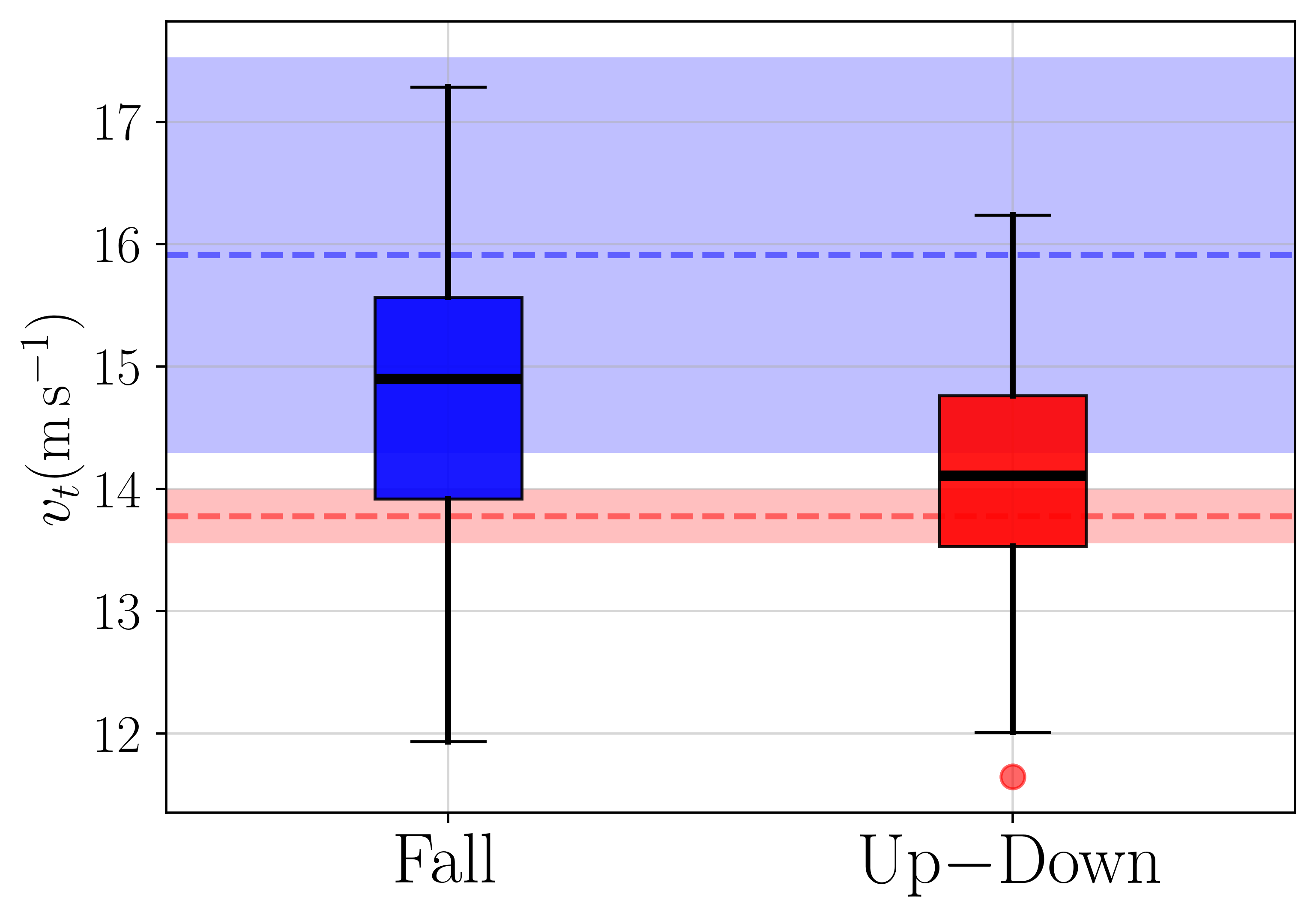
Figure 10: Comparison of terminal velocities $v_{t}$ from the Fall (blue) and Up$-$Down (red) experiments. The boxes represent the interquartile range (IQR) of the individual trials, with the black horizontal line indicating the median value. The whiskers extend to the minimum and maximum observed values, and individual points denote outliers. The shaded areas and dashed horizontal lines correspond to the best-fit results from the Grouped Data, illustrating the terminal velocity along with uncertainties derived from the WLS method.

Although simple, the theoretical model and experimental setup provided valuable insights into the dynamics of turbulent drag. The combination of a straightforward experimental procedure—relying solely on a smartphone’s built-in accelerometer—and basic data analysis methods allowed for the investigation of a nuanced and intricate subject in an accessible way. Despite the variability introduced by manual drops and the uncontrolled nature of the experiments, the results align well with expectations for turbulent flow. This study demonstrates how a simple, hands-on experiment using a smartphone accelerometer can effectively explore complex topics, integrating theoretical understanding with practical data collection and analysis.

6 Future Work

This study provides an initial exploration of the dynamics of a falling smartphone under air drag, integrating theoretical modeling and experimental data. However, several avenues remain open for further investigation. In this section, we propose potential extensions, including the integration of video analysis with accelerometer data, analysis of the terminal phase of motion, generalization of the drag force model, and considerations of tilt. These developments offer valuable pedagogical opportunities, deepening the understanding of experimental physics and data analysis.

6.1 Video Analysis and Combined Analysis

A natural extension of this work involves integrating video analysis with the accelerometer data [19]. Video analysis provides a complementary data source, capturing the smartphone’s motion in real-time and offering position-time data during the fall. Two methods can be applied to these data sets.

The first method involves analyzing the accelerometer and video data separately to obtain independent estimates of the terminal velocity. This enables a consistency check between the two approaches, validating the results and identifying discrepancies that may arise from experimental uncertainties or data processing differences.

The second method consists of a single model fit that integrates both data sets into a unified likelihood function, with the terminal velocity treated as a shared parameter. This combined analysis provides a more consistent estimation and highlights the added value of integrating multiple sources beyond what separate analyses can offer.

Combined data analysis introduces valuable techniques that are not only fundamental in experimental physics but also increasingly relevant across a wide range of fields, where integrating multiple sources of information plays a crucial role in modern decision-making and problem-solving.

6.2 In Search of the Terminal Phase

An important feature of the turbulent drag model is its potential to identify the final stage of motion through the last change in the concavity of the proper acceleration curve (see Fig. 1). Although this phenomenon was not detected in the current dataset, future experiments can be designed to capture and analyze this transition.

Two simple methods could increase the likelihood of capturing this change in concavity: increasing the height of the drop and using materials with higher drag coefficients. While a greater drop height would provide more time to capture this final phase, it also increases the risk of the smartphone’s orientation shifting during the fall. Similarly, adding surfaces that increase drag, such as cardboard, could further slow the object and reduce its terminal velocity, but at the cost of a trade-off between surface area and mass.

Furthermore, future studies may explore varying the shape and orientation of the object to gain deeper insights into how these factors influence drag during the final phase of motion. Refining the experimental setup to enhance sensitivity to subtle changes in acceleration could provide valuable insights into the behavior of objects as they approach terminal velocity under turbulent flow conditions, contributing to a more comprehensive understanding of drag dynamics.

6.3 Generalized Drag Force

We propose generalizing the drag force model by allowing the exponent $n$ in Eq. (8) to be a free parameter. In our current analysis, we fixed $n=1$, corresponding to the turbulent drag model.

While this approach lacks physical motivation, it serves as a valuable pedagogical tool for exploring the limits of our model and the nature of air resistance. Notably, the turbulent model $(n=1)$ itself has some limitations, such as the discontinuity in the snap, the second derivative of proper acceleration, at the apex, as discussed in Section 2.3.

This generalized model has four free parameters: initial velocity $(v_{0})$, terminal velocity $(v_{t})$, offset $(\Delta a)$, and the drag exponent $(n)$, which is the new free parameter. The added complexity of the model requires careful handling of potential correlations between parameters, especially between $n$ and $v_{t}$. To improve the stability of the numerical analysis, one useful strategy is to fit the combination $v_{t}^{n}$ instead of $v_{t}$ directly. This reparameterization helps decouple the effects of $n$ and $v_{t}$, reducing correlations and enhancing the robustness of the fitting process.

Comparing the generalized model with the fixed turbulent model provides an opportunity to introduce the concept of model selection. To perform this comparison, we propose using model selection criteria such as the Akaike Information Criterion (AIC) and the Bayesian Information Criterion (BIC) [20]. These criteria offer a quantitative framework for comparing models with different numbers of parameters, balancing goodness of fit against model complexity. By analyzing the AIC and BIC values of the generalized and turbulent models, we can determine whether the additional complexity introduced by freeing the exponent $n$ is justified by an improved fit.

It’s important to note that this generalization is only feasible for the Up$-$Down experimental setup. The Fall experiments lack the constraining power necessary to reliably fit an additional free parameter. In contrast, the Up$-$Down configuration, with its inclusion of both upward and downward motion and the critical information provided by the apex, offers sufficient constraints to allow for a meaningful determination of $n$.

6.4 Effects of Tilt

In the original model for the smartphone’s fall developed in Section 2, we assumed that the device’s screen remained perfectly aligned with the direction of motion, strictly along the vertical axis, such that $\hat{z}_{p}\cdot\hat{z}=1$. However, in practice, the smartphone may exhibit a tilt (i.e., the screen is not perfectly aligned with the direction of motion) due to its manual release, which introduces additional complexities into the analysis. Here, we continue to assume that the smartphone’s motion is purely vertical, $\vec{v}=v\hat{z}$, but with the presence of a constant tilt.

The tilt angle $\theta$ is defined as the angle between the smartphone’s screen and the vertical direction, such that $\hat{z}_{p}\cdot\hat{z}=\cos\theta$. The drag force $\vec{F}_{D}$ opposes the smartphone’s motion relative to the air, and in the Earth-fixed reference frame, is given by:

$$\vec{F}_{D}=-k|v|^{n}v\cos\theta\,\hat{z},$$ (23)

where the term $\cos\theta$ accounts for the reduced effective area exposed to the airflow due to the tilt. The drag constant $k$ remains unchanged compared to the case without tilt.

Applying Newton’s second law, the total acceleration along the vertical axis becomes:

$$a=-g-\frac{k}{m}|v|^{n}v\cos\theta.$$ (24)

At terminal velocity, where $a=0$, the drag force balances the gravitational force. From this condition, the terminal velocity with tilt is given by:

$$v_{t_{\theta}}=\frac{v_{t}}{(\cos\theta)^{1/(n+1)}},$$ (25)

where $v_{t}$ is the terminal velocity when the smartphone is perfectly aligned with the direction of motion ($\theta=0$), following the same notation as in the original model (see Eq. (6)). As the tilt angle increases, the terminal velocity $v_{t_{\theta}}$ increases, approaching infinity (free fall) when $\theta=90^{\circ}$.

The equation for the total acceleration in the Earth’s reference frame can be rewritten as:

$$a=-g\left(1+\frac{|v|^{n}v}{v_{t}^{n+1}}\cos\theta\right).$$ (26)

The smartphone’s accelerometer measures acceleration along its own $z_{p}$-axis, which is perpendicular to the screen. Since the drag force acts along the vertical $z$-axis, the force must be projected onto the $z_{p}$-axis. The proper acceleration measured by the accelerometer is thus given by:

$$a_{p}=-g\frac{|v|^{n}v}{v_{t}^{n+1}}\cos^{2}\theta.$$ (27)

The additional $\cos\theta$ factor arises from projecting the drag force onto the smartphone’s axis, making the effect of tilt on the accelerometer reading proportional to $\cos^{2}\theta$.

The difference in how $\cos\theta$ appears in the equations for total acceleration $a$ and proper acceleration $a_{p}$ introduces challenges in the fitting process. While $a_{p}$ depends on $\cos^{2}\theta$, the total acceleration $a$ is only linearly dependent on $\cos\theta$. In both cases, $\cos\theta$ is tied to the terminal velocity, creating a degeneracy between these parameters. This degeneracy, combined with the differing functional forms of $\cos\theta$ in the equations, makes it difficult to treat the tilt as an independent adjustable parameter. As a result, incorporating the tilt into the analysis introduces significant complexity, requiring more sophisticated fitting techniques and potentially leading to less robust parameter estimations.

Appendix A Drag Coefficient

The drag coefficient $(C_{D})$ is a dimensionless quantity that measures the resistance an object experiences when moving through a fluid, such as air. At terminal velocity, the drag force balances the object’s weight, allowing us to calculate the drag coefficient for turbulent flow using the following relation [21]:

$$C_{D}=\frac{2mg}{\rho Av_{t}^{2}},$$ (28)

where $m=0.170\,\text{kg}$ is the mass of the smartphone, $g=9.8\,\text{m}\,\text{s}^{-2}$ is the gravitational acceleration, $\rho=1.184\,\text{kg}\,\text{m}^{-3}$ is the air density, and $A=LH$ is the cross-sectional area of the smartphone, with $L=7.55\,\text{cm}$ and $H=15.79\,\text{cm}$ [10]. The parameter $v_{t}$ represents the terminal velocity obtained in Section 4.

The drag coefficient was calculated for both the Fall and Up$-$Down experiments using the terminal velocity values from individual trials and the Grouped Data. The results are summarized as follows:

• Fall: $1.12\pm 0.21$ (individual trials) and $0.93\pm 0.19$ (Grouped Data).

• Up$-$Down: $1.22\pm 0.21$ (individual trials) and $1.24\pm 0.04$ (Grouped Data).

The drag coefficient values from individual trials show a small difference of approximately 8% between the Fall and Up$-$Down experiments, indicating reasonable consistency across both setups. However, the Grouped Data amplifies this difference to 25%.

Fig. 11 provides a visual comparison of the drag coefficient values. The plot displays the interquartile range (IQR) and median for the individual trials, along with the best-fit results from the Grouped Data, including uncertainties (represented by the shaded areas and dashed horizontal lines).

The drag coefficients obtained in this study range between 0.8 and 1.7, aligning with reported values for similar objects, typically around $C_{D}=1.14$ [22]. These results suggest that, despite the variability between trials, our simple experimental setup provides reliable estimates comparable to more complex fluid dynamics studies.

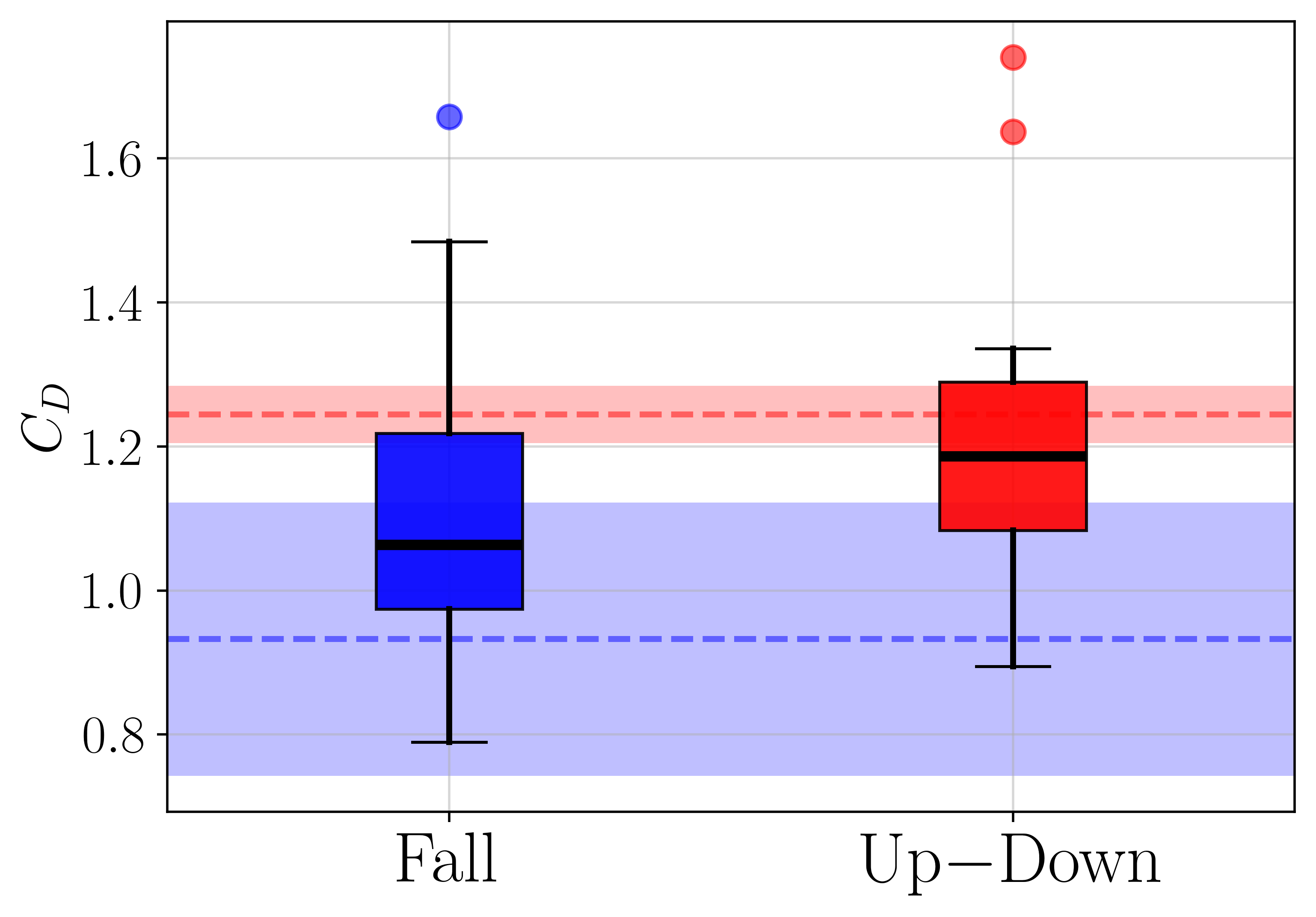
Figure 11: Comparison of drag coefficient $C_{D}$ for the Fall (blue) and Up$-$Down (red) experiments. The boxes represent the interquartile range (IQR) of the individual trials, with the black horizontal line marking the median value. The whiskers extend to the minimum and maximum observed values, and outliers are indicated by individual points. The shaded areas and dashed horizontal lines represent the best-fit results from the Grouped Data, showing the drag coefficient with uncertainties derived from the WLS method.

References

- [1] V. Pagonis, D. Guerra, S. Chauduri, B. Hornbecker, and N. Smiths, The Physics Teacher 35, 364-368 (1997).
- [2] P. Mohazzabi, The Physics Teacher 49, 89-90 (2011).
- [3] P. Mohazzabi, The Physics Teacher 56, 168-169 (2018).
- [4] P.K. Kundu and I.M. Cohen, Fluid Mechanics (Academic Press, California, 2010), 2 ed.
- [5] J.D. Anderson, Fundamentals of Aerodynamics (McGraw-Hill Education, New York, 2010), 6 ed.
- [6] G. W. Parker, American Journal of Physics 45, 606-610 (1977).
- [7] P. A. Wijaya, U. Fauzi, and F. D. E. Latief, Physics Education, 54, 055009 (2019).
- [8] P. Vogt and J. Kuhn, The Physics Teacher 50, 182-183 (2012).
- [9] D. Eager, A. Pendrill, and N. Reistad, European Journal of Physics 37, 065008 (2016).
- [10] GSMArena, Asus ZenFone Max Pro (M2) ZB631KL Specifications, accessed: 2024-10-02.
- [11] S. Staacks, S. Hutz, H. Heinke, and C. Stampfer, Physics Education 53, 045009 (2018).
- [12] Bosch Sensortec, BMI160 - Low power inertial measurement unit, accessed: 2024-10-02.
- [13] M. Monteiro, C. Stari, C. Cabeza, and A. C. Marti, American Journal of Physics 89, 477-481 (2021).
- [14] S. F. Odenwald and C. M. Bailey, IEEE Access 7, 148131-148141 (2019).
- [15] E. Cui and X. Zhang, Encyclopedia of Aerospace Engineering (R. Blockley and W. Shyy, 2010).
- [16] Engineers Edge, Viscosity of Air, Dynamic and Kinematic, accessed: 2024-10-02.
- [17] H. Akima, Journal of the ACM 17, 589–602 (1970).
- [18] G. Cowan, Statistical Data Analysis (Oxford University Press, New York, 1998), 1 ed.
- [19] M. Monteiro, C. Cabeza, and A. C. Marti, Revista Brasileira de Ensino de Física 37, 1303 (2015).
- [20] A. R. Liddle, Monthly Notices of the Royal Astronomical Society: Letters 377, L74-L78 (2007).
- [21] K. W. Ragland, M. A. Mason, and W. W. Simmons, Journal of Fluids Engineering 105, 174-178 (1983).
- [22] R. Fail, J. A. Lawford, and R. C. W. Eyre, UK Ministry of Aviation Technical report (1957).