Heavy-Tailed Diffusion Models
Abstract
Diffusion models achieve state-of-the-art generation quality across many applications, but their ability to capture rare or extreme events in heavy-tailed distributions remains unclear. In this work, we show that traditional diffusion and flow-matching models with standard Gaussian priors fail to capture heavy-tailed behavior. We address this by repurposing the diffusion framework for heavy-tail estimation using multivariate Student-t distributions. We develop a tailored perturbation kernel and derive the denoising posterior based on the conditional Student-t distribution for the backward process. Inspired by -divergence for heavy-tailed distributions, we derive a training objective for heavy-tailed denoisers. The resulting framework introduces controllable tail generation using only a single scalar hyperparameter, making it easily tunable for diverse real-world distributions. As specific instantiations of our framework, we introduce t-EDM and t-Flow, extensions of existing diffusion and flow models that employ a Student-t prior. Remarkably, our approach is readily compatible with standard Gaussian diffusion models and requires only minimal code changes. Empirically, we show that our t-EDM and t-Flow outperform standard diffusion models in heavy-tail estimation on high-resolution weather datasets in which generating rare and extreme events is crucial.
1 Introduction
In many real-world applications, such as weather forecasting, rare or extreme events—like hurricanes or heatwaves—can have disproportionately larger impacts than more common occurrences. Therefore, building generative models capable of accurately capturing these extreme events is critically important (Gründemann et al., 2022). However, learning the distribution of such data from finite samples is particularly challenging, as the number of empirically observed tail events is typically small, making accurate estimation difficult.
One promising approach is to use heavy-tailed distributions, which allocate more density to the tails than light-tailed alternatives. In popular generative models like Normalizing Flows (Rezende & Mohamed, 2016) and Variational Autoencoders (VAEs) (Kingma & Welling, 2022), recent works address heavy-tail estimation by learning a mapping from a heavy-tailed prior to the target distribution (Jaini et al., 2020; Kim et al., 2024b).
While these works advocate for heavy-tailed base distributions, their application to real-world, high-dimensional datasets remains limited, with empirical results focused on small-scale or toy datasets. In contrast, diffusion models (Ho et al., 2020; Song et al., 2020; Lipman et al., 2023) have demonstrated excellent synthesis quality in large-scale applications. However, it is unclear whether diffusion models with Gaussian priors can effectively model heavy-tailed distributions without significant modifications.
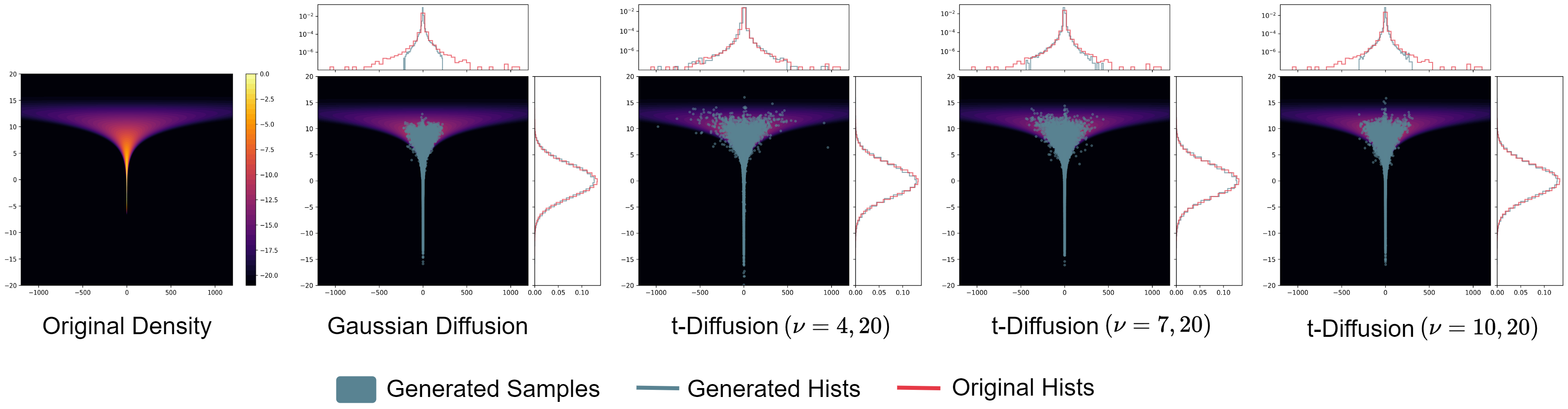
In this work, we first demonstrate through extensive experiments that traditional diffusion models—even with proper normalization, preconditioning, and noise schedule design (see Section 4)—fail to accurately capture the heavy-tailed behavior in target distributions (see Fig. 1 for a toy example). We hypothesize that, in high-dimensional spaces, the Gaussian distribution in standard diffusion models tends to concentrate on a spherical narrow shell, thereby neglecting the tails. To address this, we adopt the multivariate Student-t distribution as the base noise distribution, with its degrees of freedom providing controllability over tail estimation. Consequently, we reformulate the denoising diffusion framework using multivariate Student-t distributions by designing a tailored perturbation kernel and deriving the corresponding denoiser. Moreover, we draw inspiration from the -power Divergences (Eguchi, 2021; Kim et al., 2024a) for heavy-tailed distributions to formulate the learning problem for our heavy-tailed denoiser.
We extend widely adopted diffusion models, such as EDM (Karras et al., 2022) and straight-line flows (Lipman et al., 2023; Liu et al., 2022), by introducing their Student-t counterparts: t-EDM and t-Flow. We derive the corresponding SDEs and ODEs for modeling heavy-tailed distributions. Through extensive experiments on the HRRR dataset (Dowell et al., 2022), we train both unconditional and conditional versions of these models. The results show that standard EDM struggles to capture tails and extreme events, whereas t-EDM performs significantly better in modeling such phenomena. To summarize, we present,
-
•
Heavy-tailed Diffusion Models. We repurpose the diffusion model framework for heavy-tail estimation by formulating both the forward and reverse processes using multivariate Student-t distributions. The denoiser is learned by minimizing the -power divergence (Kim et al., 2024a) between the forward and reverse posteriors.
-
•
Continuous Counterparts. We derive continuous formulations for heavy-tailed diffusion models and provide a principled approach to constructing ODE and SDE samplers. This enables the instantiation of t-EDM and t-Flow as heavy-tailed analogues to standard diffusion and flow models.
-
•
Empirical Results. Experiments on the HRRR dataset (Dowell et al., 2022), a high-resolution dataset for weather modeling, show that t-EDM significantly outperforms EDM in capturing tail distributions for both unconditional and conditional tasks.
-
•
Theoretical Connections. To theoretically justify the effectiveness of our approach, we present several theoretical connections between our framework and existing work in diffusion models and robust statistical estimators (Futami et al., 2018).
2 Background
As prerequisites underlying our method, we briefly summarize Gaussian diffusion models (as introduced in (Ho et al., 2020; Sohl-Dickstein et al., 2015)) and multivariate Student-t distributions.
2.1 Diffusion Models
Diffusion models define a forward process (usually with an affine drift and no learnable parameters) to convert data to noise. A learnable reverse process is then trained to generate data from noise. In the discrete-time setting, the training objective for diffusion models can be specified as,
| (1) |
where denotes the trajectory length while denotes the time increment between two consecutive time points. denotes the Kullback-Leibler (KL) divergence defined as, . In the objective in Eq. 1, the trajectory length is chosen to match the generative prior and the forward marginal . The second term in Eqn. 1 proposes to minimize the KL divergence between the forward posterior and the learnable posterior which corresponds to learning the denoiser (i.e. predicting a less noisy state from noise). The forward marginals, posterior, and reverse posterior are modeled using Gaussian distributions, which exhibit an analytical form of the KL divergence. The discrete-time diffusion framework can also be extended to the continuous time setting (Song et al., 2020; 2021; Karras et al., 2022). Recently, Lipman et al. (2023); Albergo et al. (2023a) proposed stochastic interpolants (or flows), which allow flexible transport between two arbitrary distributions.
2.2 Student-t Distributions
The multivariate Student-t distribution with dimensionality d, location , scale matrix and degrees of freedom is defined as,
| (2) |
where is the normalizing factor. Since the multivariate Student-t distribution has polynomially decaying density, it can model heavy-tailed distributions. Interestingly, for , the Student-t distribution is analogous to the Cauchy distribution. As , the Student-t distribution converges to the Gaussian distribution. A Student-t distributed random variable can be reparameterized as (Andrews & Mallows, 1974), , with where denotes the Chi-squared distribution.
3 Heavy-Tailed Diffusion Models
We now repurpose standard diffusion models using multivariate Student-t distributions. The main idea behind our design is the use of heavy-tailed generative priors (Jaini et al., 2020; Kim et al., 2024a) for learning a transport map towards a potentially heavy-tailed target distribution. From Eqn. 1 we note three key requirements for training diffusion models: choice of the perturbation kernel , form of the target denoising posterior and the parameterization of the learnable reverse posterior . Therefore, we begin our discussion in the context of discrete-time diffusion models and later extend to the continuous regime. This has several advantages in terms of highlighting these three key design choices, which might be obscured by the continuous-time framework of defining a forward and a reverse SDE (Karras et al., 2022) while at the same time leading to a simpler construction.
3.1 Noising Process Design with Student-t Distributions.
Our construction of the noising process involves three key steps.
-
1.
Firstly, given two consecutive noisy states and , we specify a joint distribution .
-
2.
Secondly, given , we construct the perturbation kernel which can be used as a noising process during training.
-
3.
Lastly, from Steps 1 and 2, we construct the forward denoising posterior . We will later utilize the form of to parameterize the reverse posterior.
It is worth noting that our construction of the noising process bypasses the specification of the forward transition kernel . This has the advantage that we can directly specify the form of the perturbation kernel parameters and as in Karras et al. (2022) unlike Song et al. (2020); Ho et al. (2020). We next highlight the noising process construction in more detail.
Specifiying the joint distribution . We parameterize the joint distribution as a multivariate Student-t distribution with the following form,
where are time-dependent scalar design parameters. While the choice of the parameters and determines the perturbation kernel used during training, the choice of and can affect the ODE/SDE formulation for the denoising process and will be clarified when discussing sampling.
Constructing the perturbation kernel : Given the joint distribution specified as a multivariate Student-t distribution, it follows that the perturbation kernel distribution is also a Student-t distribution (Ding, 2016) parameterized as, (proof in App. A.1). We choose the scalar coefficients and such that the perturbation kernel at time converges to a standard Student-t generative prior . We discuss practical choices of and in Section 3.5.
Estimating the reference denoising posterior. Given the joint distribution and the perturbation kernel , the denoising posterior can be specified as (see Ding (2016)),
| (3) |
| (4) |
where . Next, we formulate the training objective for heavy-tailed diffusions.
3.2 Parameterization of the Reverse Posterior
Following Eqn. 3, we parameterize the reverse (or the denoising) posterior distribution as:
| (5) |
where the denoiser mean is further parameterized as follows:
| (6) |
While we adopt the "-prediction" parameterization (Karras et al., 2022), it is also possible to parameterize the posterior mean as an -prediction objective instead (Ho et al., 2020) (See App. A.2). Lastly, when parameterizing the reverse posterior scale, we drop the data-dependent coefficient This aligns with prior works in diffusion models (Ho et al., 2020; Song et al., 2020; Karras et al., 2022) where it is common to only parameterize the denoiser mean. However, heteroskedastic modeling of the denoiser is possible in our framework and could be an interesting direction for future work. Next, we reformulate the training objective in Eqn. 1 for heavy-tailed diffusions.
3.3 Training with Power Divergences
The optimization objective in Eqn. 1 primarily minimizes the KL-Divergence between a given pair of distributions. However, since we parameterize the distributions in Eqn. 1 using multivariate Student-t distributions, using the KL-Divergence might not be a suitable choice of divergence. This is because computing the KL divergence for Student-t distributions does not exhibit a closed-form expression. An alternative is the -Power Divergence (Eguchi, 2021; Kim et al., 2024a) defined as,
where, like Kim et al. (2024a), we set for the remainder of our discussion. Moreover, and represent the -power entropy and cross-entropy, respectively. Interestingly, the -Power divergence between two multivariate Student-t distributions, and , can be tractably computed in closed form and is defined as (see Kim et al. (2024a) for a proof),
| (7) | ||||
Therefore, analogous to Eqn. 1, we minimize the following optimization objective,
| (8) |
Here, we note a couple of caveats. Firstly, while replacing the KL-Divergence with the -Power Divergence in the objective in Eqn. 1 might appear to be due to computational convenience, the -power divergence has several connections with robust estimators (Futami et al., 2018) in statistics and provides a tunable parameter which can be used to control the model density assigned at the tail (see Section 5). Secondly, while the objective in Eqn. 1 is a valid ELBO, the objective in Eq. 8 is not. However, the following result provides a connection between the two objectives (see proof in App. A.3),
Proposition 1.
Therefore, under the limit , the standard diffusion model framework becomes a special case of our proposed framework. Moreover, for , this also explains the tail estimation moving towards Gaussian diffusion for an increasing (See Fig. 1 for an illustration.)
Simplifying the Training Objective. Plugging the form of the forward posterior in Eqn. 3, the reverse posterior in the optimization objective in Eqn. 8, we obtain the following simplified training loss (proof in App. A.4),
| (9) |
Intuitively, the form of our training objective is similar to existing diffusion models (Ho et al., 2020; Karras et al., 2022). However, the only difference lies in sampling the noisy state from a Student-t distribution based perturbation kernel instead of a Gaussian distribution. Next, we discuss sampling from our proposed framework under discrete and continuous-time settings.
| Component | Gaussian Diffusion | (Ours) t-Diffusion |
|---|---|---|
| Perturbation Kernel () | ||
| Forward Posterior () | ||
| Reverse Posterior () | ||
| Divergence Measure |
3.4 Sampling
Discrete-time Sampling. For discrete-time settings, we can simply perform ancestral sampling from the learned reverse posterior distribution . Therefore, following simple re-parameterization, an ancestral sampling update can be specified as,
Continuous-time Sampling. Due to recent advances in accelerating sampling in continuous-time diffusion processes (Pandey et al., 2024a; Zhang & Chen, 2023; Lu et al., 2022; Song et al., 2022a; Xu et al., 2023a), we reformulate discrete-time dynamics in heavy-tailed diffusions to the continuous time regime. More specifically, we present a family of continuous-time processes in the following result (Proof in App. A.5).
Proposition 2.
The posterior parameterization in Eqn. 5 induces the following continuous-time dynamics,
where and are scalar-valued functions, is a scaling coefficient such that the following condition holds,
where denote the first-order time-derivatives of the perturbation kernel parameters and respectively and the differential .
Based on the result in Proposition 2, it is possible to construct deterministic/stochastic samplers for heavy-tailed diffusions. It is worth noting that the SDE in Eqn. 10 implies adding heavy-tailed stochastic noise during inference (Bollerslev, 1987). Next, we provide specific instantiations of the generic sampler in Eq. 10.
Sampler Instantiations. We instantiate the continuous-time SDE in Eqn. 10 by setting and . Consequently, . In this case, the SDE in Eqn. 10 reduces to an ODE, which can be represented as,
| (11) |
Summary. To summarize our theoretical framework, we present an overview of the comparison between Gaussian diffusion models and our proposed heavy-tailed diffusion models in Table 1.
3.5 Specific Instantiations: t-EDM
Karras et al. (2022) highlight several design choices during training and sampling which significantly improve sample quality while reducing sampling budget for image datasets like CIFAR-10 (Krizhevsky, 2009) and ImageNet (Deng et al., 2009). With a similar motivation, we reformulate the perturbation kernel as and denote the resulting diffusion model as t-EDM.
Training. During training, we set the perturbation kernel, , parameters , . Moreover, we parameterize the denoiser as
Our denoiser parameterization is similar to Karras et al. (2022) with the difference that coefficients like additionally depend on . We include full derivations in Appendix A.6. Consequently, our denoising loss can be specified as follows:
| (12) |
where is a weighting function set to .
Sampling. Interestingly, it can be shown that the ODE in Eqn. 11 is equivalent to the deterministic dynamics presented in Karras et al. (2022) (See Appendix A.7 for proof). Consequently, we choose and during sampling, further simplifying the dynamics in Eqn. 11 to
We adopt the timestep discretization schedule and the choice of the numerical ODE solver (Heun’s method (Ascher & Petzold, 1998)) directly from EDM.
Figure 2 illustrates the ease of transitioning from a Gaussian diffusion framework (EDM) to t-EDM. Under standard settings, transitioning to t-EDM requires as few as two lines of code change, making our method readily compatible with existing implementations of Gaussian diffusion models.
4 Experiments
To assess the effectiveness of the proposed heavy-tailed diffusion and flow models, we demonstrate experiments using real-world weather data for both unconditional and conditional generation tasks. We include full experimental details in App. C.
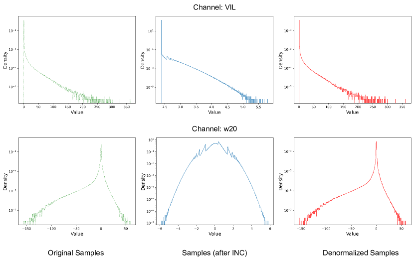
Datasets. We adopt the High-Resolution Rapid Refresh (HRRR) (Dowell et al., 2022) dataset, which is an operational archive of the US km-scale forecasting model. Among multiple dynamical variables in the dataset that exhibit heavy-tailed behavior, based on their dynamic range, we only consider the Vertically Integrated Liquid (VIL) and Vertical Wind Velocity at level 20 (denoted as w20) channels (see App. C.1 for more details). It is worth noting that the VIL and w20 channels have heavier right and left tails, respectively (See Fig. 6)
Tasks and Metrics. We consider both unconditional and conditional generative tasks relevant to weather and climate science. For unconditional modeling, we aim to generate the VIL and w20 physical variables in the HRRR dataset. For conditional modeling, we aim to generatively predict the hourly evolution of the target variable for the next lead-time () hour-ahead evolution of VIL and w20 based on information only at the current state time ; see more details in the appendix and see Pathak et al. (2024) for discussion of why hour-ahead, km-scale atmospheric prediction is a stochastic physical task appropriate for conditional generative models. To quantify the empirical performance of unconditional modeling, we rely on comparing 1-d statistics of generated and train/test set samples. More specifically, for quantitative analysis, we report the Kurtosis Ratio (KR), the Skewness Ratio (SR), and the Kolmogorov-Smirnov (KS)-2 sample statistic (at the tails) between the generated and train/test set samples. For qualitative analysis, we compare 1-d histograms between generated and train/test set samples. For the conditional task, we adopt standard probabilistic prediction score metrics such as the Continuous Ranked Probability Score (CRPS), the Root-Mean Squared Error (RMSE), and the skill-spread ratio (SSR); see, e.g., Mardani et al. (2023a); Srivastava et al. (2023). A more detailed explanation of our evaluation protocol is provided in App. C.
Methods and Baselines. In addition to standard diffusion (EDM (Karras et al., 2022)) and flow models (Albergo et al., 2023a) based on Gaussian priors, we introduce two additional baselines that are variants of EDM. To account for the high dynamic-range often exhibited by heavy-tailed distributions, we include Inverse CDF Normalization (INC) as an alternative data preprocessing step to z-score normalization. Using the former reduces dynamic range significantly and can make the data distribution closer to Gaussian. We denote this preprocessing scheme combined with standard EDM training as EDM + INC. Alternatively, we could instead modulate the noise levels used during EDM training as a function of the dynamic range of the input channel while keeping the data preprocessing unchanged. The main intuition is to use more heavy-tailed noise for large values. We denote this modulating scheme as Per-Channel Preconditioning (PCP) and denote the resulting baseline as EDM + PCP. We elaborate on these baselines in more detail in App. C.1.2
| VIL (Train) | VIL (Test) | w20 (Train) | w20 (Test) | ||||||||||||
|---|---|---|---|---|---|---|---|---|---|---|---|---|---|---|---|
| Method | KR | SR | KS | KR | SR | KS | KR | SR | KS | KR | SR | KS | |||
| Baselines | EDM | 210.11 | 10.79 | 0.997 | 45.35 | 5.23 | 0.991 | 12.59 | 0.89 | 0.991 | 5.01 | 0.38 | 0.978 | ||
| +INC | 11.33 | 2.29 | 0.987 | 1.70 | 0.74 | 0.95 | 1.80 | 0.18 | 0.909 | 0.23 | 0.13 | 0.763 | |||
| +PCP | 2.12 | 0.72 | 0.800 | 0.31 | 0.09 | 0.522 | 2.17 | 0.70 | 0.838 | 0.40 | 0.24 | 0.648 | |||
| Ours | t-EDM | 3 | 1.06 | 0.43 | 0.431 | 0.54 | 0.23 | 0.114 | 3 | 2.44 | 0.65 | 0.683 | 0.52 | 0.21 | 0.286 |
| t-EDM | 5 | 29.66 | 4.07 | 0.955 | 5.73 | 1.68 | 0.888 | 5 | 8.55 | 1.77 | 0.895 | 3.22 | 1.03 | 0.774 | |
| t-EDM | 7 | 24.35 | 4.14 | 0.959 | 4.57 | 1.72 | 0.908 | 7 | 7.03 | 1.58 | 0.82 | 2.55 | 0.89 | 0.622 | |
4.1 Unconditional Generation
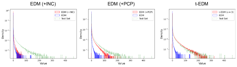
We assess the effectiveness of different methods on unconditional modeling for the VIL and w20 channels in the HRRR dataset. Fig. 3 qualitatively compares 1-d histograms of sample intensities between different methods for the VIL channel. We make the following key observations. Firstly, though EDM (with additional tricks like noise conditioning) can improve tail coverage, t-EDM covers a broader range of extreme values in the test set. Secondly, in addition to better dynamic range coverage, t-EDM qualitatively performs much better in capturing the density assigned to intermediate intensity levels under the model. We note similar observations from our quantitative results in Table 2, where t-EDM outperforms other baselines on the KS metric, implying our model exhibits better tail estimation over competing baselines for both the VIL and w20 channels. More importantly, unlike traditional Gaussian diffusion models like EDM, t-EDM enables controllable tail estimation by varying , which could be useful when modeling a combination of channels with diverse statistical properties. On the contrary, standard diffusion models like EDM do not have such controllability. Lastly, we present similar quantitative results for t-Flow in Table 3. We present additional results for unconditional modeling in App. C.1
| VIL (Train) | VIL (Test) | w20 (Train) | w20 (Test) | ||||||||||||||
| Method | KR | SR | KS | KR | SR | KS | KR | SR | KS | KR | SR | KS | |||||
| Baselines |
|
0.46 | 0.09 | 0.897 | 0.67 | 0.52 | 0.704 | 2.03 | 0.36 | 0.294 | 0.34 | 0.01 | 0.384 | ||||
| Ours | t-Flow | 3 | 1.39 | 0.37 | 0.711 | 0.47 | 0.27 | 0.275 | 5 | 1.08 | 0.21 | 0.333 | 0.07 | 0.42 | 0.512 | ||
| t-Flow | 5 | 3.30 | 0.75 | 0.857 | 0.05 | 0.07 | 0.633 | 7 | 3.24 | 0.36 | 0.259 | 0.87 | 0.01 | 0.300 | |||
| t-Flow | 7 | 3.36 | 0.84 | 0.844 | 0.04 | 0.02 | 0.603 | 9 | 5.47 | 0.41 | 0.478 | 1.86 | 0.034 | 0.289 | |||
4.2 Conditional Generation
Next, we consider the task of conditional modeling, where we aim to predict the hourly evolution of a target variable for the next lead time () based on the current state at time . Table 4 illustrates the performance of EDM and t-EDM on this task for the VIL and w20 channels. We make the following key observations. Firstly, for both channels, t-EDM exhibits better CRPS and SSR scores, implying better probabilistic forecast skills and ensemble than EDM. Moreover, while t-EDM exhibits under-dispersion for VIL, while it is well-calibrated for w20, with its SSR close to an ideal score of 1. On the contrary, the baseline EDM model exhibits under-dispersion for both channels, thus implying overconfident predictions. Secondly, in addition to better calibration, t-EDM is better at tail estimation (as measured by the KS statistic) for the underlying conditional distribution. Lastly, we notice that different values of the parameter are optimal for different channels, which suggests a more data-driven approach to learning the optimal directly. We present additional results for conditional modeling in App. C.2.
| VIL (Test) | w20 (Test) | ||||||||||
| Method | CRPS | RMSE | SSR () | KS | CRPS | RMSE | SSR () | KS | |||
| Baselines | EDM | 1.696 | 4.473 | 0.203 | 0.715 | 0.304 | 0.664 | 0.865 | 0.345 | ||
| Ours | t-EDM | 3 | 1.649 | 4.526 | 0.255 | 0.419 | 3 | 0.295 | 0.734 | 1.045 | 0.111 |
| t-EDM | 5 | 1.609 | 4.361 | 0.305 | 0.665 | 5 | 0.301 | 0.674 | 0.901 | 0.323 | |
5 Discussion and Theoretical Insights
To conclude, we propose a framework for constructing heavy-tailed diffusion models and demonstrate their effectiveness over traditional diffusion models on unconditional and conditional generation tasks for a high-resolution weather dataset. Here, we highlight some theoretical connections that help gain insights into the effectiveness of our proposed framework while establishing connections with prior work.
Exploring distribution tails during sampling. The ODE in Eq. 11 can re-formulated as,
| (13) |
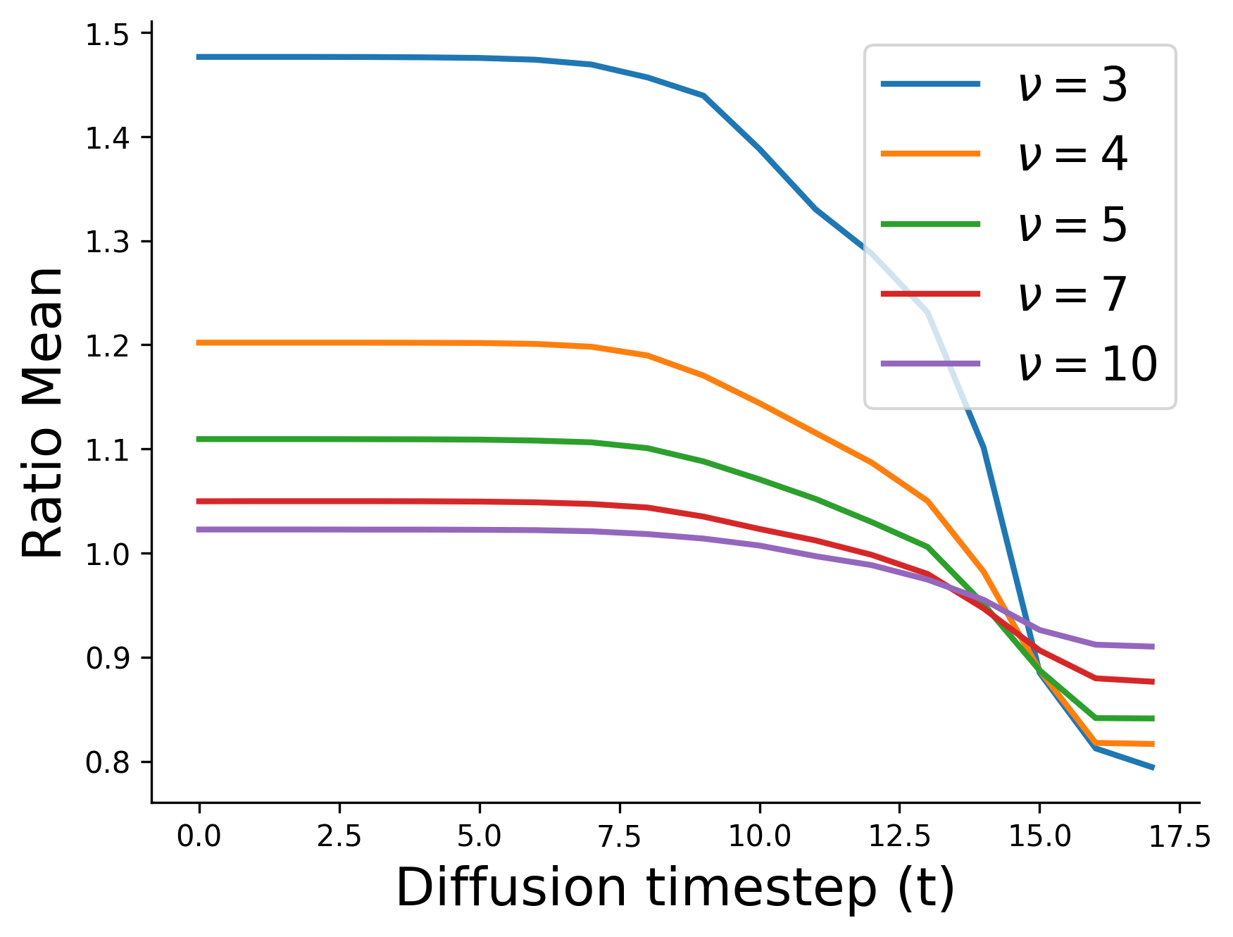
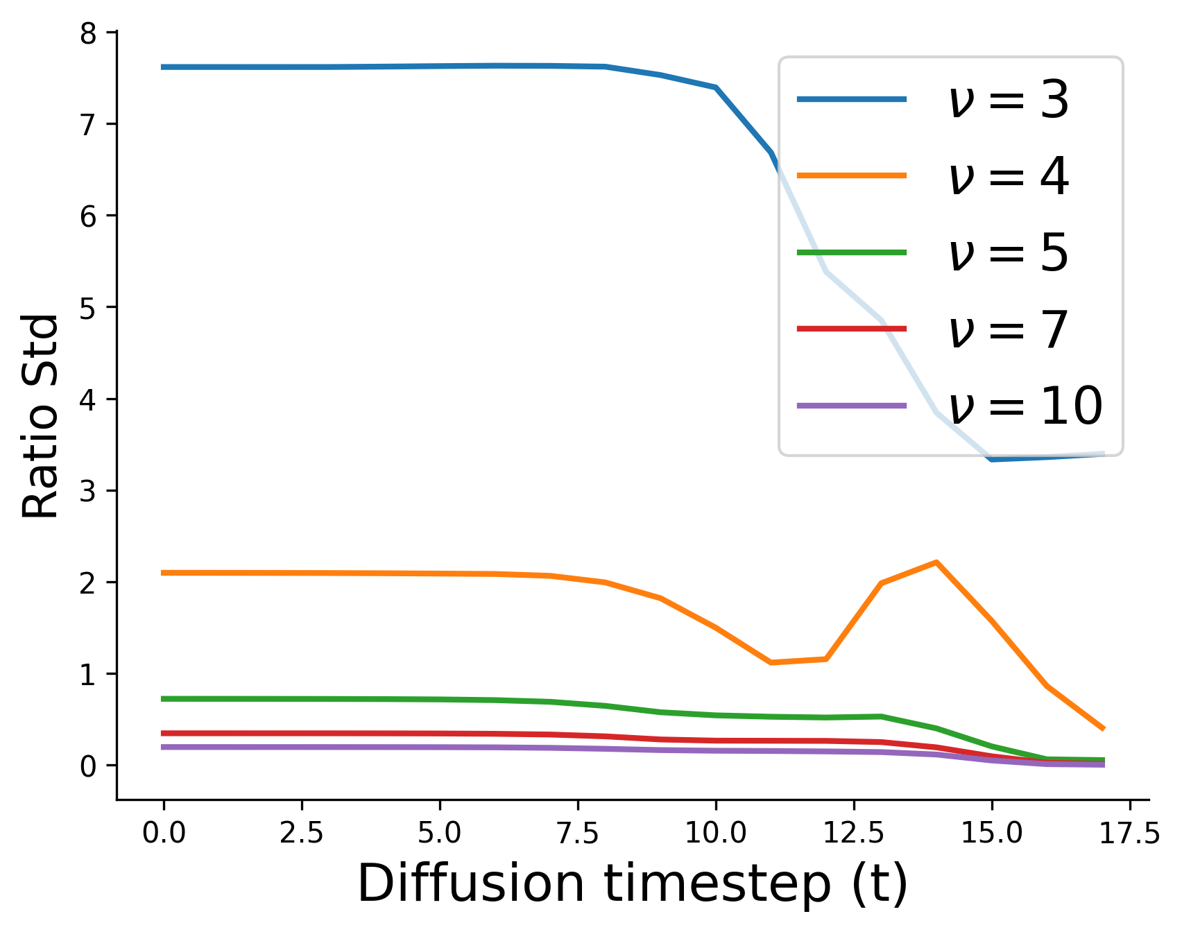
where . By formulating the ODE in terms of the score function, we can gain some intuition into the effectiveness of our model in modeling heavy-tailed distributions. Figure 4 illustrates the variation of the mean and variance of the multiplier along the diffusion trajectory across 1M samples generated from our toy models. Interestingly, as the value of decreases, the mean and variance of this multiplier increase significantly, which leads to large score multiplier weights. We hypothesize that this behavior allows our proposed model to explore more diverse regions during sampling (more details in App. A.10).
Enabling efficient tail coverage during training. The optimization objective in Eq. 8 has several connections with robust statistical estimators. More specifically, it can be shown that (proof in App. A.11),
where and denote the forward () and reverse diffusion posteriors (), respectively. Intuitively, the coefficient weighs the likelihood gradient, , and can be set accordingly to ignore or consider outliers when modeling the data distribution. Specifically, when , the model would learn to ignore outliers (Futami et al., 2018; Fujisawa & Eguchi, 2008; Basu et al., 1998) since data points on the tails would be assigned low likelihood. On the contrary, a negative value of (as is the case in this work since we set ), the model can assign more weights to capture these extreme values.
Reproducibility Statement
Ethics Statement
We develop a generative framework for modeling heavy-tailed distributions and demonstrate its effectiveness for scientific applications. In this context, we do not think our model poses a risk of misinformation or other ethical biases associated with large-scale image synthesis models. However, we would like to point out that similar to other generative models, our model can sometimes hallucinate predictions for certain channels, which could impact downstream applications like weather forecasting.
References
- Albergo et al. (2023a) Michael S Albergo, Nicholas M Boffi, and Eric Vanden-Eijnden. Stochastic interpolants: A unifying framework for flows and diffusions. arXiv preprint arXiv:2303.08797, 2023a.
- Albergo et al. (2023b) Michael S. Albergo, Nicholas M. Boffi, and Eric Vanden-Eijnden. Stochastic interpolants: A unifying framework for flows and diffusions, 2023b. URL https://arxiv.org/abs/2303.08797.
- Andrews & Mallows (1974) D. F. Andrews and C. L. Mallows. Scale mixtures of normal distributions. Journal of the Royal Statistical Society. Series B (Methodological), 36(1):99–102, 1974. ISSN 00359246. URL http://www.jstor.org/stable/2984774.
- Ascher & Petzold (1998) Uri M. Ascher and Linda R. Petzold. Computer Methods for Ordinary Differential Equations and Differential-Algebraic Equations. Society for Industrial and Applied Mathematics, Philadelphia, PA, 1998. doi: 10.1137/1.9781611971392. URL https://epubs.siam.org/doi/abs/10.1137/1.9781611971392.
- Basu et al. (1998) Ayanendranath Basu, Ian R Harris, Nils L Hjort, and MC Jones. Robust and efficient estimation by minimising a density power divergence. Biometrika, 85(3):549–559, 1998.
- Bollerslev (1987) Tim Bollerslev. A conditionally heteroskedastic time series model for speculative prices and rates of return. The Review of Economics and Statistics, 69(3):542–547, 1987. ISSN 00346535, 15309142. URL http://www.jstor.org/stable/1925546.
- Brooks et al. (2011) Steve Brooks, Andrew Gelman, Galin Jones, and Xiao-Li Meng. Handbook of Markov Chain Monte Carlo. Chapman and Hall/CRC, May 2011. ISBN 9780429138508. doi: 10.1201/b10905. URL http://dx.doi.org/10.1201/b10905.
- Chai & Draxler (2014) Tianfeng Chai and Roland R Draxler. Root mean square error (rmse) or mean absolute error (mae)?–arguments against avoiding rmse in the literature. Geoscientific Model Development, 7(3):1247–1250, 2014.
- Chung et al. (2022) Hyungjin Chung, Jeongsol Kim, Michael Thompson Mccann, Marc Louis Klasky, and Jong Chul Ye. Diffusion posterior sampling for general noisy inverse problems. In The Eleventh International Conference on Learning Representations, 2022.
- Deng et al. (2009) Jia Deng, Wei Dong, Richard Socher, Li-Jia Li, Kai Li, and Li Fei-Fei. Imagenet: A large-scale hierarchical image database. In 2009 IEEE Conference on Computer Vision and Pattern Recognition, pp. 248–255, 2009. doi: 10.1109/CVPR.2009.5206848.
- Ding (2016) Peng Ding. On the conditional distribution of the multivariate distribution, 2016. URL https://arxiv.org/abs/1604.00561.
- Dockhorn et al. (2022) Tim Dockhorn, Arash Vahdat, and Karsten Kreis. Score-based generative modeling with critically-damped langevin diffusion, 2022. URL https://arxiv.org/abs/2112.07068.
- Dosovitskiy & Brox (2016) Alexey Dosovitskiy and Thomas Brox. Generating images with perceptual similarity metrics based on deep networks, 2016. URL https://arxiv.org/abs/1602.02644.
- Dowell et al. (2022) David C. Dowell, Curtis R. Alexander, Eric P. James, Stephen S. Weygandt, Stanley G. Benjamin, Geoffrey S. Manikin, Benjamin T. Blake, John M. Brown, Joseph B. Olson, Ming Hu, Tatiana G. Smirnova, Terra Ladwig, Jaymes S. Kenyon, Ravan Ahmadov, David D. Turner, Jeffrey D. Duda, and Trevor I. Alcott. The high-resolution rapid refresh (hrrr): An hourly updating convection-allowing forecast model. part i: Motivation and system description. Weather and Forecasting, 37(8):1371 – 1395, 2022. doi: 10.1175/WAF-D-21-0151.1. URL https://journals.ametsoc.org/view/journals/wefo/37/8/WAF-D-21-0151.1.xml.
- Eguchi (2021) Shinto Eguchi. Chapter 2 - pythagoras theorem in information geometry and applications to generalized linear models. In Angelo Plastino, Arni S.R. Srinivasa Rao, and C.R. Rao (eds.), Information Geometry, volume 45 of Handbook of Statistics, pp. 15–42. Elsevier, 2021. doi: https://doi.org/10.1016/bs.host.2021.06.001. URL https://www.sciencedirect.com/science/article/pii/S0169716121000225.
- Esser et al. (2024) Patrick Esser, Sumith Kulal, Andreas Blattmann, Rahim Entezari, Jonas Müller, Harry Saini, Yam Levi, Dominik Lorenz, Axel Sauer, Frederic Boesel, Dustin Podell, Tim Dockhorn, Zion English, Kyle Lacey, Alex Goodwin, Yannik Marek, and Robin Rombach. Scaling rectified flow transformers for high-resolution image synthesis, 2024. URL https://arxiv.org/abs/2403.03206.
- Fujisawa & Eguchi (2008) Hironori Fujisawa and Shinto Eguchi. Robust parameter estimation with a small bias against heavy contamination. Journal of Multivariate Analysis, 99(9):2053–2081, 2008. ISSN 0047-259X. doi: https://doi.org/10.1016/j.jmva.2008.02.004. URL https://www.sciencedirect.com/science/article/pii/S0047259X08000456.
- Futami et al. (2018) Futoshi Futami, Issei Sato, and Masashi Sugiyama. Variational inference based on robust divergences, 2018. URL https://arxiv.org/abs/1710.06595.
- Gründemann et al. (2022) Gaby Joanne Gründemann, Nick van de Giesen, Lukas Brunner, and Ruud van der Ent. Rarest rainfall events will see the greatest relative increase in magnitude under future climate change. Communications Earth &; Environment, 3(1), October 2022. ISSN 2662-4435. doi: 10.1038/s43247-022-00558-8. URL http://dx.doi.org/10.1038/s43247-022-00558-8.
- Guo et al. (2015) H. Guo, J.-C. Golaz, L. J. Donner, B. Wyman, M. Zhao, and P. Ginoux. Clubb as a unified cloud parameterization: Opportunities and challenges. Geophysical Research Letters, 42(11):4540–4547, 2015. doi: https://doi.org/10.1002/2015GL063672. URL https://agupubs.onlinelibrary.wiley.com/doi/abs/10.1002/2015GL063672.
- Heusel et al. (2018) Martin Heusel, Hubert Ramsauer, Thomas Unterthiner, Bernhard Nessler, and Sepp Hochreiter. Gans trained by a two time-scale update rule converge to a local nash equilibrium, 2018. URL https://arxiv.org/abs/1706.08500.
- Ho et al. (2020) Jonathan Ho, Ajay Jain, and Pieter Abbeel. Denoising diffusion probabilistic models. Advances in Neural Information Processing Systems, 33:6840–6851, 2020.
- Hutchinson (1990) M.F. Hutchinson. A stochastic estimator of the trace of the influence matrix for laplacian smoothing splines. Communications in Statistics - Simulation and Computation, 19(2):433–450, 1990. doi: 10.1080/03610919008812866. URL https://doi.org/10.1080/03610919008812866.
- Jaini et al. (2020) Priyank Jaini, Ivan Kobyzev, Yaoliang Yu, and Marcus Brubaker. Tails of lipschitz triangular flows, 2020. URL https://arxiv.org/abs/1907.04481.
- Karras et al. (2022) Tero Karras, Miika Aittala, Timo Aila, and Samuli Laine. Elucidating the design space of diffusion-based generative models, 2022. URL https://arxiv.org/abs/2206.00364.
- Kim et al. (2024a) Juno Kim, Jaehyuk Kwon, Mincheol Cho, Hyunjong Lee, and Joong-Ho Won. -variational autoencoder: Learning heavy-tailed data with student’s t and power divergence, 2024a. URL https://arxiv.org/abs/2312.01133.
- Kim et al. (2024b) Juno Kim, Jaehyuk Kwon, Mincheol Cho, Hyunjong Lee, and Joong-Ho Won. $t^3$-variational autoencoder: Learning heavy-tailed data with student’s t and power divergence. In The Twelfth International Conference on Learning Representations, 2024b. URL https://openreview.net/forum?id=RzNlECeoOB.
- Kingma & Welling (2022) Diederik P Kingma and Max Welling. Auto-encoding variational bayes, 2022. URL https://arxiv.org/abs/1312.6114.
- Krizhevsky (2009) Alex Krizhevsky. Learning multiple layers of features from tiny images. pp. 32–33, 2009. URL https://www.cs.toronto.edu/~kriz/learning-features-2009-TR.pdf.
- Laszkiewicz et al. (2022) Mike Laszkiewicz, Johannes Lederer, and Asja Fischer. Marginal tail-adaptive normalizing flows, 2022. URL https://arxiv.org/abs/2206.10311.
- Lipman et al. (2023) Yaron Lipman, Ricky T. Q. Chen, Heli Ben-Hamu, Maximilian Nickel, and Matthew Le. Flow matching for generative modeling. In International Conference on Learning Representations, 2023. URL https://openreview.net/forum?id=PqvMRDCJT9t.
- Liu et al. (2022) Xingchao Liu, Chengyue Gong, and Qiang Liu. Flow straight and fast: Learning to generate and transfer data with rectified flow, 2022. URL https://arxiv.org/abs/2209.03003.
- Lu et al. (2022) Cheng Lu, Yuhao Zhou, Fan Bao, Jianfei Chen, Chongxuan Li, and Jun Zhu. Dpm-solver: A fast ode solver for diffusion probabilistic model sampling in around 10 steps, 2022. URL https://arxiv.org/abs/2206.00927.
- Mardani et al. (2023a) Morteza Mardani, Noah Brenowitz, Yair Cohen, Jaideep Pathak, Chieh-Yu Chen, Cheng-Chin Liu, Arash Vahdat, Karthik Kashinath, Jan Kautz, and Mike Pritchard. Residual corrective diffusion modeling for km-scale atmospheric downscaling. arXiv preprint arXiv:2309.15214, 2023a.
- Mardani et al. (2023b) Morteza Mardani, Jiaming Song, Jan Kautz, and Arash Vahdat. A variational perspective on solving inverse problems with diffusion models. In The Twelfth International Conference on Learning Representations, 2023b.
- Mardani et al. (2024) Morteza Mardani, Noah Brenowitz, Yair Cohen, Jaideep Pathak, Chieh-Yu Chen, Cheng-Chin Liu, Arash Vahdat, Mohammad Amin Nabian, Tao Ge, Akshay Subramaniam, Karthik Kashinath, Jan Kautz, and Mike Pritchard. Residual corrective diffusion modeling for km-scale atmospheric downscaling, 2024. URL https://arxiv.org/abs/2309.15214.
- Massey (1951) Frank J. Massey. The kolmogorov-smirnov test for goodness of fit. Journal of the American Statistical Association, 46(253):68–78, 1951. ISSN 01621459, 1537274X. URL http://www.jstor.org/stable/2280095.
- Neal (2003) Radford M. Neal. Slice sampling. The Annals of Statistics, 31(3):705 – 767, 2003. doi: 10.1214/aos/1056562461. URL https://doi.org/10.1214/aos/1056562461.
- Pandey & Mandt (2023) Kushagra Pandey and Stephan Mandt. A complete recipe for diffusion generative models, 2023. URL https://arxiv.org/abs/2303.01748.
- Pandey et al. (2022) Kushagra Pandey, Avideep Mukherjee, Piyush Rai, and Abhishek Kumar. Diffusevae: Efficient, controllable and high-fidelity generation from low-dimensional latents, 2022. URL https://arxiv.org/abs/2201.00308.
- Pandey et al. (2024a) Kushagra Pandey, Maja Rudolph, and Stephan Mandt. Efficient integrators for diffusion generative models. In The Twelfth International Conference on Learning Representations, 2024a. URL https://openreview.net/forum?id=qA4foxO5Gf.
- Pandey et al. (2024b) Kushagra Pandey, Ruihan Yang, and Stephan Mandt. Fast samplers for inverse problems in iterative refinement models, 2024b. URL https://arxiv.org/abs/2405.17673.
- Pathak et al. (2024) Jaideep Pathak, Yair Cohen, Piyush Garg, Peter Harrington, Noah Brenowitz, Dale Durran, Morteza Mardani, Arash Vahdat, Shaoming Xu, Karthik Kashinath, and Michael Pritchard. Kilometer-scale convection allowing model emulation using generative diffusion modeling, 2024. URL https://arxiv.org/abs/2408.10958.
- Podell et al. (2023) Dustin Podell, Zion English, Kyle Lacey, Andreas Blattmann, Tim Dockhorn, Jonas Müller, Joe Penna, and Robin Rombach. Sdxl: Improving latent diffusion models for high-resolution image synthesis, 2023. URL https://arxiv.org/abs/2307.01952.
- Rezende & Mohamed (2016) Danilo Jimenez Rezende and Shakir Mohamed. Variational inference with normalizing flows, 2016. URL https://arxiv.org/abs/1505.05770.
- Rombach et al. (2022) Robin Rombach, Andreas Blattmann, Dominik Lorenz, Patrick Esser, and Björn Ommer. High-resolution image synthesis with latent diffusion models, 2022. URL https://arxiv.org/abs/2112.10752.
- Shariatian et al. (2024) Dario Shariatian, Umut Simsekli, and Alain Durmus. Denoising lévy probabilistic models, 2024. URL https://arxiv.org/abs/2407.18609.
- Singhal et al. (2023) Raghav Singhal, Mark Goldstein, and Rajesh Ranganath. Where to diffuse, how to diffuse, and how to get back: Automated learning for multivariate diffusions, 2023. URL https://arxiv.org/abs/2302.07261.
- Skilling (1989) John Skilling. The Eigenvalues of Mega-dimensional Matrices, pp. 455–466. Springer Netherlands, Dordrecht, 1989. ISBN 978-94-015-7860-8. doi: 10.1007/978-94-015-7860-8_48. URL https://doi.org/10.1007/978-94-015-7860-8_48.
- Sohl-Dickstein et al. (2015) Jascha Sohl-Dickstein, Eric Weiss, Niru Maheswaranathan, and Surya Ganguli. Deep unsupervised learning using nonequilibrium thermodynamics. In International Conference on Machine Learning, pp. 2256–2265. PMLR, 2015.
- Song et al. (2022a) Jiaming Song, Chenlin Meng, and Stefano Ermon. Denoising diffusion implicit models, 2022a. URL https://arxiv.org/abs/2010.02502.
- Song et al. (2022b) Jiaming Song, Arash Vahdat, Morteza Mardani, and Jan Kautz. Pseudoinverse-guided diffusion models for inverse problems. In International Conference on Learning Representations, 2022b.
- Song et al. (2020) Yang Song, Jascha Sohl-Dickstein, Diederik P Kingma, Abhishek Kumar, Stefano Ermon, and Ben Poole. Score-based generative modeling through stochastic differential equations. In International Conference on Learning Representations, 2020.
- Song et al. (2021) Yang Song, Conor Durkan, Iain Murray, and Stefano Ermon. Maximum likelihood training of score-based diffusion models, 2021. URL https://arxiv.org/abs/2101.09258.
- Srivastava et al. (2023) Prakhar Srivastava, Ruihan Yang, Gavin Kerrigan, Gideon Dresdner, Jeremy McGibbon, Christopher Bretherton, and Stephan Mandt. Precipitation downscaling with spatiotemporal video diffusion. arXiv preprint arXiv:2312.06071, 2023.
- Vincent (2011) Pascal Vincent. A connection between score matching and denoising autoencoders. Neural Computation, 23(7):1661–1674, 2011. doi: 10.1162/NECO_a_00142.
- Wilks (2011) Daniel S Wilks. Statistical methods in the atmospheric sciences, volume 100. Academic press, 2011.
- Xu et al. (2023a) Yilun Xu, Mingyang Deng, Xiang Cheng, Yonglong Tian, Ziming Liu, and Tommi S. Jaakkola. Restart sampling for improving generative processes. In Thirty-seventh Conference on Neural Information Processing Systems, 2023a. URL https://openreview.net/forum?id=wFuemocyHZ.
- Xu et al. (2023b) Yilun Xu, Ziming Liu, Yonglong Tian, Shangyuan Tong, Max Tegmark, and Tommi Jaakkola. Pfgm++: Unlocking the potential of physics-inspired generative models. In International Conference on Machine Learning, pp. 38566–38591. PMLR, 2023b.
- Yoon et al. (2023) Eunbi Yoon, Keehun Park, Sungwoong Kim, and Sungbin Lim. Score-based generative models with lévy processes. In Thirty-seventh Conference on Neural Information Processing Systems, 2023. URL https://openreview.net/forum?id=0Wp3VHX0Gm.
- Zhang & Chen (2023) Qinsheng Zhang and Yongxin Chen. Fast sampling of diffusion models with exponential integrator, 2023. URL https://arxiv.org/abs/2204.13902.
Appendix A Proofs
A.1 Derivation of the Perturbation Kernel
Proof.
By re-parameterization of the distribution , we have,
| (14) |
This implies that the conditional distribution . Therefore, following properties of gaussian distributions, . Therefore, from reparameterization,
| (15) |
which implies that . This completes the proof. ∎
A.2 On the Posterior Parameterization
The perturbation kernel for Student-t diffusions is parameterized as,
| (16) |
Using re-parameterization,
| (17) |
During inference, given a noisy state , we have the following estimation problem,
| (18) |
Therefore, the task of denoising can be posed as either estimating or . With this motivation, the posterior can be parameterized appropriately. Recall the form of the forward posterior
| (19) |
| (20) |
where . Further simplifying the mean ,
| (21) | ||||
| (22) | ||||
| (23) |
Therefore, the mean of the reverse posterior can be parameterized as,
| (24) | ||||
| (25) |
where is learned using a parametric estimator . This corresponds to the -prediction parameterization presented in Eq. 6 in the main text. Alternatively, From Eqn. 18,
| (26) | ||||
| (27) | ||||
| (28) | ||||
| (29) |
where is learned using a parametric estimator . This corresponds to the -prediction parameterization (Ho et al., 2020).
A.3 Proof of Proposition 1
We restate the proposition here for convenience,
Proposition 1.
Proof.
We present our proof in two parts:
-
1.
Firstly, we establish the following relation between the -Power Divergence and the KL-Divergence between two distributions and .
(30) - 2.
Relation between and . The -Power Divergence as stated in (Kim et al., 2024a) assumes the following form:
| (31) |
where , and,
| (32) |
For subsequent analysis, we assume . Under this assumption, we simplify as follows. By definition,
| (33) | ||||
| (34) | ||||
| (35) | ||||
| (36) | ||||
| (37) | ||||
| (38) |
Using the approximation for a small in the above equation, we have,
| (39) | ||||
| (40) |
where we have used the approximation in the above equation. This is justified since is assumed to be small enough. Therefore, we have,
| (41) |
Similarly, we now obtain an approximation for the power-cross entropy as follows. By definition,
| (42) | ||||
| (43) | ||||
| (44) | ||||
| (45) |
From Eqn. 41, it follows that,
| (46) |
Therefore,
| (47) | ||||
| (48) |
where the above result follows from the logarithmic series and ignores the terms of order or higher. Plugging the approximation in Eqn. 48 in Eqn. 45, we have,
| (49) | ||||
| (50) |
Therefore,
| (51) | ||||
| (52) | ||||
| (53) | ||||
| (54) |
This establishes the relationship between the KL and -Power divergence between two distributions. Therefore, for two distributions and , the difference in the magnitude of and is of the order of . In the limit of , the . This concludes the first part of our proof.
Equivalence between the objectives under . For and a finite-dimensional dataset with , it follows that implies . Moreover, in the limit of , the multivariate Student-t distribution converges to a Gaussian distribution. As already shown in the previous part, under this limit, converges to . Therefore, under this limit, the optimization objective in Eqn. 8 converges to the standard DDPM objective in Eqn. 1. This completes the proof. ∎
A.4 Derivation of the simplified denoising loss
Here, we derive the simplified denoising loss presented in Eq. 9 in the main text. We specifically consider the term in Eq. 8. The -power divergence between two Student-t distributions is given by,
| (55) | ||||
where . Recall, the definitions of the forward denoising posterior,
| (56) |
| (57) |
and the reverse denoising posterior,
| (58) |
where the denoiser mean is further parameterized as follows:
| (59) |
Since we only parameterize the mean of the reverse posterior, the majority of the terms in the -power divergence are independent of and can be ignored (or treated as scalar coefficients). Therefore,
| (60) | ||||
| (61) | ||||
| (62) |
For better sample quality, it is common to ignore the scalar multiple in prior works (Ho et al., 2020; Song et al., 2020). Therefore, ignoring the time-dependent scalar multiple,
| (63) |
Therefore, the final loss function can be stated as,
| (64) |
A.5 Proof of Proposition 2
We restate the proposition here for convenience,
Proposition 2.
The posterior parameterization in Eqn. 5 induces the following continuous-time dynamics,
| (65) |
where and are scalar-valued functions, is a scaling coefficient such that the following condition holds,
| (66) |
where denote the first-order time-derivatives of the perturbation kernel parameters and respectively and the differential .
Proof.
We start by writing a single sampling step from our learned posterior distribution. Recall
| (67) |
where (using the -prediction parameterization in App. A.2),
| (68) |
From re-parameterization, we have,
| (69) | ||||
| (70) |
Moreover, we choose the posterior scale to be the same as the forward posterior i.e.
| (71) |
This implies,
| (72) |
Substituting this form of into Eqn. 70, we have,
| (73) | ||||
| (74) | ||||
| (75) | ||||
| (76) |
where in the above equation we use the first-order approximation . Next, we make the following design choices:
-
1.
Firstly, we assume the following form of the reverse posterior variance :
(77) where and represents a time-varying scaling factor chosen empirically which can be used to vary the noise injected at each sampling step. It is worth noting that a positive (as indicated in the definition of g) is a consequence of a monotonically increasing noise schedule in diffusion model design.
-
2.
Secondly, we make the following design choice:
(78) where
With these two design choices, Eqn. 76 simplifies as:
| (79) | ||||
| (80) | ||||
| (81) | ||||
| (82) | ||||
| (83) |
In the limit of :
| (84) |
which gives the required SDE formulation for the diffusion posterior sampling. Next, we discuss specific choices of and .
On the choice of and : Recall our design choices:
| (85) |
| (86) |
Substituting the value of from the first design choice to the second yields the following condition:
| (87) |
This concludes the proof. It is worth noting that the above equation provides two degrees of freedom, i.e., we can choose two variables among and automatically determine the third. However, it is more convenient to choose and , since both these quantities should be positive. Different choices of these quantities yield different instantiations of the SDE in Eqn. 84 as illustrated in the main text. ∎
A.6 Deriving the Denoiser Preconditioner for t-EDM
Recall our denoiser parameterization,
| (88) |
Karras et al. (2022) highlight the following design choices, which we adopt directly.
-
1.
Derive based on constraining the input variance to 1
-
2.
Derive and to constrain output variance to 1 and additionally minimizing to bound scaling errors in .
The coefficient can be derived by setting the network inputs to have unit variance. Therefore,
| (89) | |||||
| (90) | |||||
| (91) | |||||
| (92) |
The coefficients and can be derived by setting the training target to have unit variance. Similar to Karras et al. (2022) our training target can be specified as:
| (93) |
| (94) | |||||
| (95) | |||||
| (96) | |||||
| (97) | |||||
| (98) | |||||
| (99) |
Lastly, setting to minimize , we obtain,
| (100) |
Consequently can be specified as:
| (101) |
A.7 Equivalence with the EDM ODE
Similar to Karras et al. (2022), we start by deriving the optimal denoiser for the denoising loss function. Moreover, we reformulate the form of the perturbation kernel as by setting and . The denoiser loss can then be specified as follows,
| (102) | ||||
| (103) | ||||
| (104) | ||||
| (105) |
where the last result follows from assuming as the empirical data distribution. Thus, the optimal denoiser can be specified by setting . Therefore,
| (106) |
Consequently,
| (107) | ||||
| (108) | ||||
| (109) |
The optimal denoiser , can be obtained from Eq. 109 as,
| (110) |
We can further simplify the optimal denoiser as,
| (111) | ||||
| (112) | ||||
| (113) |
Next, recall the ODE dynamics (Eqn. 11) in our formulation,
| (114) |
Reparameterizing the above ODE by setting and ,
| (115) | ||||
| (116) | ||||
| (117) | ||||
| (118) |
Lastly, since Karras et al. (2022) propose to train the denoiser using unscaled noisy state, from Eqn. 113, we can re-write the above ODE as,
| (119) |
The form of the ODE in Eqn. 119 is equivalent to the ODE presented in Karras et al. (2022) (Algorithm 1 line 4 in their paper). This concludes the proof.
A.8 Conditional Vector Field for t-Flow
Here, we derive the conditional vector field for the t-Flow interpolant. Recall, the interpolant in t-Flow is derived as follows,
| (120) |
It follows that,
| (121) |
Moreover, following Eq. 2.10 in Albergo et al. (2023b), the conditional vector field can be defined as,
| (122) |
From Eqns. 121 and 122, the conditional vector field can be simplified as,
| (123) |
This concludes the proof.
A.9 Connection to Denoising Score Matching
We start by defining the score for the perturbation kernel . The pdf for the perturbation kernel can be expressed as (ignoring the normalization constant):
| (124) |
Therefore,
| (125) | ||||
| (126) |
Denoting for convenience, we have,
| (127) |
In Denoising Score Matching (DSM) (Vincent, 2011), the following objective is minimized,
| (128) |
for some loss weighting function . Parameterizing the score estimator as:
| (129) |
With this parameterization of and some choice of , the DSM objective can be further simplified as follows,
| (130) | ||||
| (131) |
where , which is equivalent to a scaled version of the simplified denoising loss Eq. 9. This concludes the proof. As an additional caveat, the score parameterization in Eq. 129 depends on , which can be approximated during inference as,
A.10 ODE Reformulation and Connections to Inverse Problems.
Recall the ODE dynamics in terms of the denoiser can be specified as,
| (132) |
From Eq. 129, we have,
| (133) |
where . Substituting the above result in the ODE dynamics, we obtain the reformulated ODE in Eq. 13.
| (134) |
Since the term is data-dependent, we can estimate it during inference as . Thus, the above ODE can be reformulated as,
| (135) |
Tweedie’s Estimate and Inverse Problems. Given the perturbation kernel , we have,
| (136) |
It follows that,
| (137) | ||||
| (138) | ||||
| (139) |
which gives us an estimate of the predicted at any time . Moreover, the framework can also be extended for solving inverse problems using diffusion models. More specifically, given a conditional signal , the goal is to simulate the ODE,
| (140) | ||||
| (141) |
where the above decomposition follows from and the weight represents the guidance weight of the distribution . The term can now be approximated using existing posterior approximation methods in inverse problems (Chung et al., 2022; Song et al., 2022b; Mardani et al., 2023b; Pandey et al., 2024b)
A.11 Connections to Robust Statistical Estimators
Here, we derive the expression for the gradient of the -power divergence between the forward and the reverse posteriors (denoted by and , respectively for notational convenience) i.e., . By the definition of the -power divergence,
| (142) |
| (143) |
Therefore,
| (144) |
Consequently, we next derive an expression for .
| (145) | ||||
| (146) | ||||
| (147) |
From the definition of ,
| (148) | ||||
| (149) | ||||
| (150) | ||||
| (151) | ||||
| (152) | ||||
| (153) | ||||
| (154) | ||||
| (155) | ||||
| (156) |
where we denote for notational convenience. Substituting the above result in Eq. 147, we have the following simplification,
| (157) | ||||
| (158) | ||||
| (159) | ||||
| (160) |
| (162) |
Plugging this result in Eq. 144, we have the following result,
| (163) |
This completes the proof. Intuitively, the second term inside the integral in Eq. 163 ensures unbiasedness of the gradients. Therefore, the scalar coefficient controls the weighting on the likelihood gradient and can be set accordingly to ignore or model outliers when modeling the data distribution.
Appendix B Extension to Flows
Here, we discuss an extension of our framework to flow matching models (Albergo et al., 2023a; Lipman et al., 2023) with a Student-t base distribution. More specifically, we define a straight-line flow of the form,
| (164) |
where . Intuitively, at a given time , the flow defined in Eqn. 164 linearly interpolates between data and Student-t noise. Following Albergo et al. (2023a), the conditional vector field which induces this interpolant can be specified as (proof in App. A.8)
| (165) |
We estimate by minimizing the objective
| (166) |
We refer to this flow setup as t-Flow. To generate samples from our model, we simulate the ODE in Eq. 165 using Heun’s solver. Figure 5 illustrates the ease of transitioning from a Gaussian flow to t-Flow. Similar to Gaussian diffusion, transitioning to t-Flow requires very few lines of code change, making our method readily compatible with existing implementations of flow models.
Appendix C Experimental Setup
C.1 Unconditional Modeling
C.1.1 HRRR Dataset
We adopt the High-Resolution Rapid Refresh (HRRR) (Dowell et al., 2022) dataset, which is an operational archive of the US km-scale forecasting model. Among multiple dynamical variables in the dataset that exhibit heavy-tailed behavior, based on their dynamic range, we only consider the Vertically Integrated Liquid (VIL) and Vertical Wind Velocity at level 20 (denoted as w20) channels. How to cope with the especially non-Gaussian nature of such physical variables on km-scales, represents an entire subfield of climate model subgrid-scale parameterization (e.g., Guo et al. (2015)). We only use data for the years for training (17.4k samples) and the data for 2021 (8.7k samples) for testing; data before 2019 are avoided owing to non-stationaries associated with periodic version changes of the HRRR. Lastly, while the HRRR dataset spans the entire US, for simplicity, we work with regional crops of size (corresponding to km over the Central US). Unless specified otherwise, we perform z-score normalization using precomputed statistics as a preprocessing step. We do not perform any additional data augmentation.
C.1.2 Baselines
Baseline 1: EDM. For standard Gaussian diffusion models, we use the recently proposed EDM (Karras et al., 2022) model, which shows strong empirical performance on various image synthesis benchmarks and has also been employed in recent work in weather forecasting and downscaling (Pathak et al., 2024; Mardani et al., 2024). To summarize, EDM employs the following denoising loss during training,
| (167) |
where the noise levels are usually sampled from a LogNormal distribution,
Baseline 2: EDM + Inverse CDF Normalization (INC). It is commonplace to perform z-score normalization as a data pre-processing step during training. However, since heavy-tailed channels usually exhibit a high dynamic range, using z-score normalization for such channels cannot fully compensate for this range, especially when working with diverse channels in downstream tasks in weather modeling. An alternative could be to use a more stronger normalization scheme like Inverse CDF normalization, which essentially involves the following key steps:
-
1.
Compute channel-wise 1-d histograms of the training data.
-
2.
Compute channel-wise empirical CDFs from the 1-d histograms computed in Step 1.
-
3.
Use the empirical CDFs from Step 2 to compute the CDF at each spatial location.
-
4.
For each spatial location with a CDF value , replace its value by the value obtained by applying the Inverse CDF operation under the standard Normal distribution.
Fig. 6 illustrates the effect of performing normalization under this scheme. As can be observed, using such a normalization scheme can greatly reduce the dynamic range of a given channel while offering reliable denormalization. Moreover, since our normalization scheme only affects data preprocessing, we leave the standard EDM model parameters unchanged for this baseline.
Baseline 3: EDM + Per Channel-Preconditioning (PCP). Another alternative to account for extreme values in the data (or high dynamic range) could be to instead add more heavy-tailed noise during training. This can be controlled by modulating the and parameters based on the dynamic range of the channel under consideration. Recall that these parameters control the domain of noise levels used during EDM model training. In this work, we use a simple heuristic to modulate these parameters based on the normalized channel dynamic range (denoted as ). More specifically, we set,
| (168) |
where RBF denotes the Radial Basis Function kernel with radius=1.0, parameter and a magnitude scaling factor . We keep fixed for all channels. Intuitively, this implies that a higher normalized dynamic range (near 1.0) corresponds to sampling the noise levels from a more heavy-tailed distribution during training. This is natural since a signal with a larger magnitude would need more amount of noise to convert it to noise during the forward diffusion process. In this work, we set , , which yields and for the VIL and w20 channels, respectively. It is worth noting that, unlike the previous baseline, we use z-score normalization as a preprocessing step for this baseline. Lastly, we keep other EDM parameters during training and sampling fixed.
Baseline 4. Gaussian Flow. Since we also extend our framework to flow matching models (Albergo et al., 2023a; Lipman et al., 2023), we also compare with a linear one-sided interpolant with a Gaussian base distribution. More specifically,
| (169) |
Similar to t-Flow (Section B), we train the Gaussian flow with the following objective,
| (170) |
C.1.3 Evaluation
Kurtosis Ratio (KR). Intuitively, sample kurtosis characterizes the heavy-tailed behavior of a distribution and represents the fourth-order moment. Higher kurtosis represents greater deviations from the central tendency, such as from outliers in the data. In this work, given samples from the underlying train/test set, we generate 20k samples from our model. We then flatten all the samples and compute empirical kurtosis for both the underlying samples from the train/test set (denoted as ) and our model (denoted as ). The Kurtosis ratio is then computed as,
| (171) |
Lower values of this ratio imply a better estimation of the underlying sample kurtosis.
Skewness Ratio (SR). Intuitively, sample skewness represents the asymmetry of a tailed distribution and represents the third-order moment. In this work, given samples from the underlying train/test set, we generate 20k samples from our model. We then flatten all the samples and compute empirical skewness for both the underlying samples from the train/test set (denoted as ) and our model (denoted as ). The Skewness ratio is then computed as,
| (172) |
Lower values of this ratio imply a better estimation of the underlying sample skewness.
Kolmogorov-Smirnov 2-Sample Test (KS). The KS (Massey, 1951) statistic measures the maximum difference between the CDFs of two distributions. For heavy-tailed distributions, evaluating the KS statistic at the tails could provide a useful measure of the efficacy of our model in estimating tails reliably. To evaluate the KS statistic at the tails, similar to prior metrics, we generate 20k samples from our model. We then flatten all samples in the generated and train/test sets, followed by retaining samples lying above the 99.9th percentile (quantifying right tails/extreme region) or below the 0.1th percentile (quantifying the left tail/extreme region). Lastly, we compute the KS statistic between the retained samples from the generated and the train/test sets individually for each tail and average the KS statistic values for both tails to obtain an average KS score. The final score estimates how well the model might capture both tails. As an exception,. for the VIL channel, we report KS scores only for the right tail due to the absence of a left tail in the underlying samples for this channel (see Fig. 6 (first column) for 1-d intensity histograms for this channel). Lower values of the KS statistic imply better density assignment at the tails by the model.
Histogram Comparisons. As a qualitative metric, comparing 1-d intensity histograms between the generated and the original samples from the train/test set can serve as a reliable proxy to assess the tail estimation capabilities of all models.
| Parameters | EDM (+INC, +PCP) | t-EDM | Flow/t-Flow | ||||||
| Preconditioner | 0 | ||||||||
| 1 | |||||||||
| 1 | |||||||||
| Training | , | ||||||||
| 1 | 1 | t | |||||||
| 1 | |||||||||
| Loss | Eq. 167 | Eq. 12 |
|
||||||
| Sampling | Solver | Heun’s (2nd order) | Heun’s (2nd order) | Heun’s (2nd order) | |||||
| ODE | Eq. 11, | Eq. 11, |
|
||||||
| Discretization | |||||||||
| Scaling: | 1 | 1 | t | ||||||
| Schedule: | t | t | 1-t | ||||||
| Hyperparameters | 1.0 | 1.0 | N/A | ||||||
|
|
||||||||
| , |
|
-1.2, 1.2 | N/A | ||||||
| , | 80, 0.002 | 80, 0.002 | 1.0, 0.01 | ||||||
| NFE | 18 | 18 | 25 | ||||||
| 7 | 7 | 7 |
C.1.4 Denoiser Architecture
We use the DDPM++ architecture from (Karras et al., 2022; Song et al., 2020). We set the base channel multiplier to 32 and the per-resolution channel multiplier to [1,2,2,4,4] with self-attention at resolution 16. The rest of the hyperparameters remain unchanged from Karras et al. (2022), which results in a model size of around 12M parameters.
C.1.5 Training
We adopt the same training hyperparameters from Karras et al. (2022) for training all models. Model training is distributed across 4 DGX nodes, each with 8 A100 GPUs, with a total batch size of 512. We train all models for a maximum budget of 60Mimg and select the best-performing model in terms of qualitative 1-D histogram comparisons.
C.1.6 Sampling
For the EDM and related baselines (INC, PCP), we use the ODE solver presented in Karras et al. (2022). For the t-EDM models, as presented in Section 3.5, our sampler is the same as EDM with the only difference in the sampling of initial latents from a Student-t distribution instead (See Fig. 2 (Right)). For Flow and t-Flow, we numerically simulate the ODE in Eq. 165 using the 2nd order Heun’s solver with the timestep discretization proposed in Karras et al. (2022). For evaluation, we generate 20k samples from each model.
We summarize our experimental setup in more detail for unconditional modeling in Table 5.
C.1.7 Extended Results on Unconditional Modeling
C.2 Conditional Modeling
| Parameter | Model Levels | Height Levels (m) |
|---|---|---|
| Zonal Wind (u) | 1,2,3,4,5,6,7,8,9,10,11,13,15,20 | 10 |
| Meridonal Wind (v) | 1,2,3,4,5,6,7,8,9,10,11,13,15,20 | 10 |
| Geopotential Height (z) | 1,2,3,4,5,6,7,8,9,10,11,13,15,20 | None |
| Humidity (q) | 1,2,3,4,5,6,7,8,9,10,11,13,15,20 | None |
| Pressure (p) | 1,2,3,4,5,6,7,8,9,10,11,13,15,20 | None |
| Temperature (t) | 1,2,3,4,5,6,7,8,9,10,11,13,15,20 | 2 |
| Radar Reflectivity (refc) | N/A | Integrated |
C.2.1 HRRR Dataset for Conditional Modeling
Similar to unconditional modeling (See App. C.1.1), we use the HRRR dataset for conditional modeling at the 128 x 128 resolution. More specifically, for a lead time of 1hr, we sample (input, output) pairs at time and , respectively. For the input, at time , we use a state vector consisting of a combination of 86 atmospheric channels (including the channel to be predicted at time ), which are summarized in Table 6. For the output, at time , we use either the Vertically Integrated Liquid (VIL) or Vertical Wind Velocity at level 20 (w20) channels, depending on the prediction task. Unless specified otherwise, we perform z-score normalization using precomputed statistics as a preprocessing step without any additional data augmentation.
C.2.2 Baselines
We adopt the standard EDM (Karras et al., 2022) for conditional modeling as our baseline.
C.2.3 Denoiser Architecture
We use the DDPM++ architecture from (Karras et al., 2022; Song et al., 2020). We set the base channel multiplier to 32 and the per-resolution channel multiplier to [1,2,2,4,4] with self-attention at resolution 16. Additionally, our noisy state is channel-wise concatenated with an 86-channel conditioning signal, increasing the total number of input channels in the denoiser to 87. The number of output channels remains 1 since we are predicting only a single VIL/w20 channel. However, the increase in the number of parameters is minimal since only the first convolutional layer in the denoiser is affected. Therefore, our denoiser is around 12M parameters. The rest of the hyperparameters remain unchanged from Karras et al. (2022).
C.2.4 Training
We adopt the same training hyperparameters from Karras et al. (2022) for training all conditional models. Model training is distributed across 4 DGX nodes, each with 8 A100 GPUs, with a total batch size of 512. We train all models for a maximum budget of 60Mimg.
C.2.5 Sampling
For both EDM and t-EDM models, we use the ODE solver presented in Karras et al. (2022). For the t-EDM models, as presented in Section 3.5, our sampler is the same as EDM with the only difference in the sampling of initial latents from a Student-t distribution instead (See Fig. 2 (Right)). For a given input conditioning state, we generate an ensemble of predictions of size 16 by randomly initializing our ODE solver with different random seeds. All other sampling parameters remain unchanged from our unconditional modeling setup (see App. C.1.6).
C.2.6 Evaluation
Root Mean Square Error (RMSE). is a standard evaluation metric used to measure the difference between the predicted values and the true values Chai & Draxler (2014). In the context of our problem, let be the true target and be the predicted value. The RMSE is defined as:
This metric captures the average magnitude of the residuals, i.e., the difference between the predicted and true values. A lower RMSE indicates better model performance, as it suggests the predicted values are closer to the true values on average. RMSE is sensitive to large errors, making it an ideal choice for evaluating models where minimizing large deviations is critical.
Continuous Ranked Probability Score (CRPS). is a measure used to evaluate probabilistic predictions Wilks (2011). It compares the entire predicted distribution with the observed data point . For a probabilistic forecast with cumulative distribution function (CDF) , and the true value , the CRPS can be formulated as follows:
where is the indicator function. Unlike RMSE, CRPS provides a more comprehensive evaluation of both the location and spread of the predicted distribution. A lower CRPS indicates a better match between the forecast distribution and the observed data. It is especially useful for probabilistic models that output a distribution rather than a single-point prediction.
Spread-Skill Ratio (SSR). is used to assess over/under-dispersion in probabilistic forecasts. Spread measures the uncertainty in the ensemble forecasts and can be represented by computing the standard deviation of the ensemble members. Skill represents the accuracy of the mean of the ensemble forecasts and can be represented by computing the RMSE between the ensemble mean and the observations.
Scoring Criterion. Since CRPS and SSR metrics are based on predicting ensemble forecasts for a given input state, we predict an ensemble of size 16 for 4000 samples from the VIL/w20 test set. We then enumerate window sizes of 16 x 16 across the spatial resolution of the generated sample (128 x 128). Since the VIL channel is quite sparse, we filter out windows with a maximum value of less than a threshold (1.0 for VIL) and compute the CRPS, SSR, and RMSE metrics for all remaining windows. As an additional caveat, we note that while it is common to roll out trajectories for weather forecasting, in this work, we only predict the target at the immediate next time step.
C.2.7 Extended Results on Conditional Modeling
C.3 Toy Experiments
| Parameters | EDM | t-EDM | |
|---|---|---|---|
| Preconditioner | |||
| Training | |||
| 1 | 1 | ||
| Loss | Eq. 2 in Karras et al. (2022) | Eq. 12 | |
| Sampling | Solver | Heun’s (2nd order) | Heun’s (2nd order) |
| ODE | Eq. 11, | Eq. 11, | |
| Discretization | |||
| Scaling: | 1 | 1 | |
| Schedule: | t | t | |
| Hyperparameters | 1.0 | 1.0 | |
| , | |||
| , | -1.2, 1.2 | -1.2, 1.2 | |
| , | 80, 0.002 | 80, 0.002 | |
| NFE | 18 | 18 | |
| 7 | 7 |
Dataset. For the toy illustration in Fig. 1, we work with the Neals Funnel dataset (Neal, 2003), which is commonly used in the MCMC literature (Brooks et al., 2011) due to its challenging geometry. The underlying generative process for Neal’s funnel can be specified as follows:
| (173) |
For training, we randomly generate 1M samples from the generative process in Eq. 173 and perform z-score normalization as a pre-processing step.
Baselines and Models. For the standard Gaussian diffusion model baseline (2nd column in Fig. 1), we use EDM with standard hyperparameters as presented in Karras et al. (2022). Consequently, for heavy-tailed diffusion models (columns 3-5 in Fig. 1), we use the t-EDM instantiation of our framework as presented in Section 3.5. Since the hyperparameter is key in our framework, we tune for each individual dimension in our toy experiments. We fix to 20 for the dimension and vary it between to illustrate controllable tail estimation along the dimension.
Denoiser Architecture. For modeling the underlying denoiser , we use a simple MLP for all toy models. At the input, we concatenate the 2-dimensional noisy state vector with the noise level . We use two hidden layers of size 64, followed by a linear output layer. This results in around 8.5k parameters for the denoiser. We share the same denoiser architecture across all toy models.
Training. We optimize the training objective in Eq. 12 for both t-EDM and EDM (See Fig. 2 (Left)). Our training hyperparameters are the same as proposed in Karras et al. (2022). We train all toy models for a fixed duration of 30M samples and choose the last checkpoint for evaluation.
Sampling. For the EDM baseline, we use the ODE solver presented in Karras et al. (2022). For the t-EDM models, as presented in Section 3.5, our sampler is the same as EDM with the only difference in the sampling of initial latents from a Student-t distribution instead (See Fig. 2 (Right)). For visualization of the generated samples in Fig. 1, we generate 1M samples for each model.
Appendix D Optimal Noise Schedule Design
In this section we discuss a strategy for choosing the parameter (denoted by in this section for notational brevity) in a more principled manner as compared to EDM (Karras et al., 2022). More specifically, our approach involves directly estimating from the empirically observed samples which circumvents the need to rely on ad-hoc choices of this parameter which can affect downstream sampler performance.
The main idea behind our approach is minimizing the statistical mutual information between datapoints from the underlying data distribution, , and their noisy counterparts . While a trivial (and non-practical) way to achieve this objective could be to set a large enough i.e. , we instead minimize the mutual information while ensuring the magnitude of to be as small as possible. Formally, our objective can be defined as,
| (174) |
As we will discuss later, minimizing this constrained objective provides a more principled way to obtain from the underlying data statistics for a specific level of mutual information desired by the user. Next, we first simplify the form of , followed by a discussion on the estimation of in the context of EDM and t-EDM. We also extend to the case of non-i.i.d noise.
Simplification of . The mutual information can be stated and simplified as follows,
| (175) | ||||
| (176) | ||||
| (177) | ||||
| (178) |
| (179) | |||
| (180) |
D.1 Design for EDM
Given the simplification in Eqn. 180, the optimization problem in Eqn. 174 reduces to the following,
| (181) |
Since at we expect the marginal distribution to converge to the generative prior (i.e. completely destory the structure of the data), we approximate . With this simplification, the Lagrangian for the optimization problem in Eqn. 174 can be specified as,
| (182) |
Setting the gradient w.r.t = 0,
| (183) |
which implies,
| (184) |
For an empirical dataset,
| (185) |
This allows us to choose a from the underlying data statistics during training or sampling. It is worth noting that the choice of the multiplier impacts the magnitude of . However, this parameter can be chosen in a principled manner. At , the estimate of the mutual information is given by:
| (186) |
which implies,
| (187) |
The above result provides a way to choose . Given the dataset stastistics, , the user can specify an acceptable level of mutual information to compute the correponding , which can then be used to find the corresponding minimum required to achieve that level of mutual information. Next, we extend this analysis to t-EDM.
D.2 Extension to t-EDM
In the case of t-EDM, we pose the optimization problem as follows,
| (188) |
where is the Gamma-power Divergence between two distributions q and p. From the definition of the -Power Divergence in Eqn. 7, we have,
| (189) |
where and Solving the optimization problem yields the following optimal ,
| (190) |
For an empirical dataset, we have the following simplification,
| (191) |
D.3 Extension to Correlated Gaussian Noise
We now extend our formulation for optimal noise schedule design to the case of correlated noise in the diffusion perturbation kernel. This is useful, especially for scientific applications where the data energy is distributed quite non-uniformly across the (data) spectrum. Let denote the data correlation matrix. Let also consider the perturbation kernel for the postitve-defintie covaraince matrix . Following the steps in equation 182, the Lagrangian for noise covariance estimation can be formulated as follows:
| (192) | ||||
| (193) | ||||
| (194) | ||||
| (195) | ||||
| (196) |
It can be shown that the optimal solution to this minimization problem is given by, , where denotes the matrix square root of . This implies that the noise energy must be distributed along the singular vectors of the correlaiton matrix, where the energy is proportional to the noise singular values. We include the proof below.
Proof. We define the objective:
| (197) |
We compute the gradient of with respect to :
| (198) |
The gradient of the first term is straightforward:
| (199) |
For the second term, using the matrix calculus identity, the gradient is:
| (200) |
Combining these results, the total gradient is:
| (201) |
Setting the gradient to zero to find the critical point:
| (202) |
| (203) |
which implies,
| (204) |
| (205) |
which completes the proof.
Appendix E Log-Likelihood for t-EDM
Here, we present a method to estimate the log-likelihood for the generated samples using the ODE solver for t-EDM (see Section 3.5). Our analysis is based on the likelihood computation in continuous-time diffusion models as discussed in Song et al. (2020) (Appendix D.2). More specifically, given a probability-flow ODE,
| (206) |
with a vector field , Song et al. (2020) propose to estimate the log-likelihood of the model as follows,
| (207) |
The divergence of the vector field is further estimated using the Skilling-Hutchinson trace estimator (Skilling, 1989; Hutchinson, 1990) as follows,
| (208) |
where usually, . For t-EDM ODE, this estimate can be further simplified as follows,
| (209) | ||||
| (210) | ||||
| (211) | ||||
| (212) | ||||
| (213) | ||||
| (214) |
where is the data dimensionality. Thus, the log-likelihood can be specified as,
| (215) |
When , the above result can be re-formulated as,
| (216) |
Moreover, using the first-order taylor series expansion
| (217) |
For a sufficiently small , higher-order terms in can be ignored since . Therefore,
| (218) | ||||
| (219) | ||||
| (220) | ||||
| (221) |
Therefore, the log-likelihood expression can be further simplified as,
| (222) | ||||
| (223) |
The advantage of this simplification is that we don’t need to rely on expensive jacobian-vector products in Eq. 215. However, since the denoiser now depends on , monte-carlo approximation of the expectation in the above equation could be computationally expensive for many samples
Appendix F Discussion and Limitations
F.1 Related Work
Connections with Denoising Score Matching. For the perturbation kernel , the denoising score matching (Vincent, 2011; Song et al., 2020) loss, , can be formulated as,
| (224) |
with the scaling factor where (proof in App. A.9). Therefore, the denoising score matching loss in our framework is equivalent to the simplified training objective in Eq. 9 scaled by a data-dependent coefficient. However, in this work, we do not explore this loss formulation and leave further exploration to future work.
Prior work in Heavy-Tailed Generative Modeling. The idea of exploring heavy-tailed priors for modeling heavy-tailed distributions has been explored in several works in the past. More specifically, Jaini et al. (2020) argue that a Lipschitz flow map cannot change the tails of the base distribution significantly. Consequently, they use a heavy-tailed prior (modeled using a Student-t distribution) as the base distribution to learn Tail Adaptive flows (TAFs), which can model the tails more accurately. In this work, we make similar observations where standard diffusion models fail to accurately model the tails of real-world distributions. Consequently, Laszkiewicz et al. (2022) assess the tailedness of each marginal dimension and set the prior accordingly. On a similar note, we note that learning the tail parameter spatially and across channels can provide greater modeling flexibility for downstream tasks and will be an important direction for future work on this problem. More recently, Kim et al. (2024b) introduce heavy-tailed VAEs (Kingma & Welling, 2022; Rezende & Mohamed, 2016) based on minimizing -power divergences (Eguchi, 2021). This is perhaps the closest connection of our method with prior work since we rely on -power divergences to minimize the divergence between heavy-tailed forward and reverse diffusion posteriors. However, VAEs often have scalability issues and tend to produce blurry artifacts (Dosovitskiy & Brox, 2016; Pandey et al., 2022). On the other hand, we work with diffusion models, which are known to scale well to large-scale modeling applications (Pathak et al., 2024; Mardani et al., 2024; Esser et al., 2024; Podell et al., 2023). In another line of work, Yoon et al. (2023) presents a framework for modeling heavy-tailed distributions using -stable Levy processes while Shariatian et al. (2024) simplify the framework proposed in Yoon et al. (2023) and instantiate it for more practical diffusion models like DDPM. In contrast, our work deals with Student-t noise, which in general (with the exceptions of Cauchy and the Gaussian distribution) is not -stable and, therefore, a distinct category of diffusion models for modeling heavy-tailed distributions. Moreover, prior works like Yoon et al. (2023); Shariatian et al. (2024) rely on empirical evidence from light-tailed variants of small-scale datasets like CIFAR-10 (Krizhevsky, 2009) and their efficacy on actual large-scale scientific datasets like weather datasets remains to be seen.
Prior work in Diffusion Models. Our work is a direct extension of standard diffusion models in the literature (Karras et al., 2022; Ho et al., 2020; Song et al., 2020). Moreover, since it only requires a few lines of code change to transition from standard diffusion models to our framework, our work is directly compatible with popular families of latent diffusion models (Pandey et al., 2022; Rombach et al., 2022) and augmented diffusion models (Dockhorn et al., 2022; Pandey & Mandt, 2023; Singhal et al., 2023). Our work is also related to prior work in diffusion models on a more theoretical level. More specifically, PFGM++ (Xu et al., 2023b) is a unique type of generative flow model inspired by electrostatic theory. It treats d-dimensional data as electrical charges in a -dimensional space, where the electric field lines define a bijection between a heavy-tailed prior and the data distribution. is a hyperparameter controlling the shape of the electric fields that define the generative mapping. In essence, their method can be seen as utilizing a perturbation kernel:
When setting , the perturbation kernel becomes equivalent to that of t-EDM, indicating the Student-t perturbation kernel can be interpreted from another physical perspective — that of electrostatic fields and charges. The authors demonstrated that using an intermediate value for (or ) leads to improved robustness compared to diffusion models (where ), due to the heavy-tailed perturbation kernel.
F.2 Limitations
While our proposed framework works well for modeling heavy-tailed data, it is not without its limitations. Firstly, while the parameter offers controllability for tail estimation using diffusion models, it also increases the tuning budget by introducing an extra hyperparameter. Moreover, for diverse data channels, tuning per channel could be key to good estimation at the tails. This could result in a combinatorial explosion with manual tuning. Therefore, learning directly from the data could be an important direction for the practical deployment of heavy-tailed diffusion models. Secondly, our evaluation protocol relies primarily on comparing the statistical properties of samples obtained by flattening the generated or train/test set samples. One disadvantage of this approach is that our current evaluation metrics ignore the structure of the generated samples. In general, developing metrics like FID (Heusel et al., 2018) to assess the perceptual quality of synthetic data for scientific domains like weather analysis remains an important future direction.
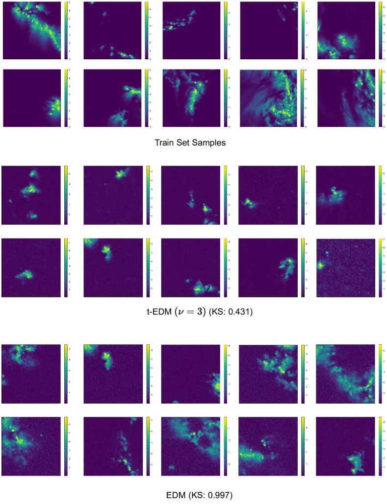
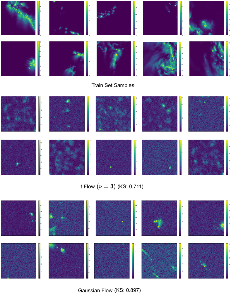
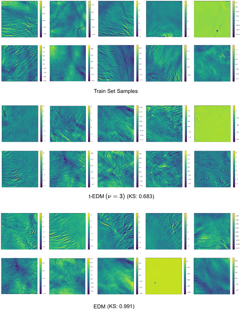
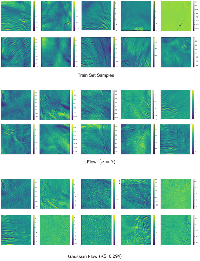
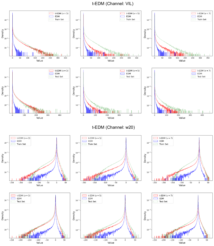
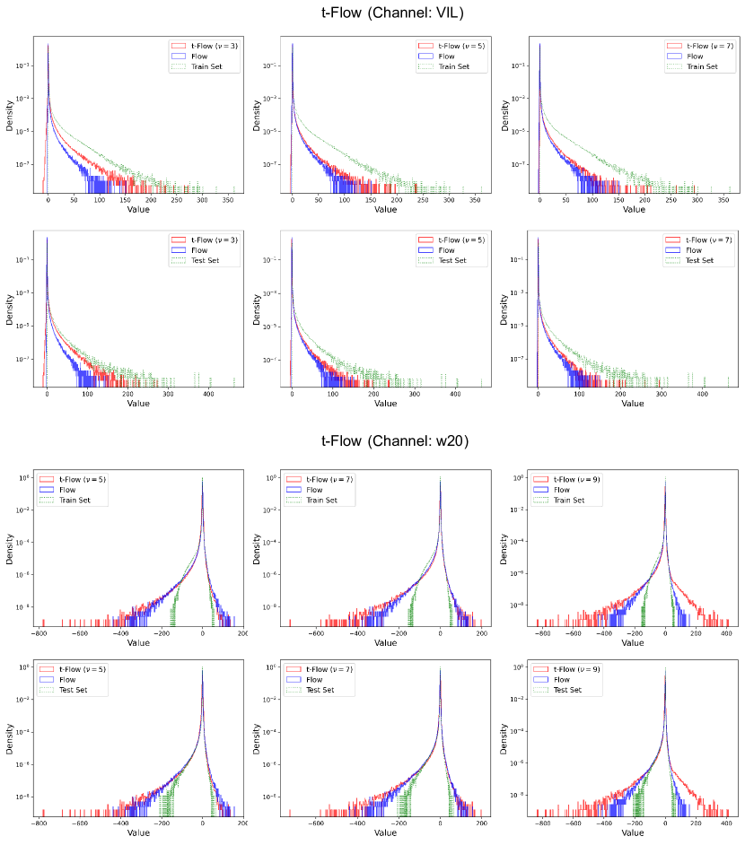
![[Uncaptioned image]](/html/2410.14171/assets/figures/nfp_vil/vil_gt_sample_0.png) Ground Truth
Ground Truth
|
|
|
|
|
||||||||
|---|---|---|---|---|---|---|---|---|---|---|---|---|
![[Uncaptioned image]](/html/2410.14171/assets/figures/nfp_vil/tedm_nu=3/sample_0/vil_pred_mean_0.png) |
![[Uncaptioned image]](/html/2410.14171/assets/figures/nfp_vil/tedm_nu=3/sample_0/ensemble/vil_pred_0_0.png) |
![[Uncaptioned image]](/html/2410.14171/assets/figures/nfp_vil/tedm_nu=3/sample_0/ensemble/vil_pred_0_1.png) |
\animategraphics[loop, autoplay, width=0.2]1figures/nfp_vil/tedm_nu=3/sample_0/ensemble/vil_pred_0_015 | |||||||||
![[Uncaptioned image]](/html/2410.14171/assets/figures/nfp_vil/tedm_nu=5/sample_0/vil_pred_mean_0.png) |
![[Uncaptioned image]](/html/2410.14171/assets/figures/nfp_vil/tedm_nu=5/sample_0/ensemble/vil_pred_0_0.png) |
![[Uncaptioned image]](/html/2410.14171/assets/figures/nfp_vil/tedm_nu=5/sample_0/ensemble/vil_pred_0_1.png) |
\animategraphics[loop, autoplay, width=0.2]1figures/nfp_vil/tedm_nu=5/sample_0/ensemble/vil_pred_0_015 | |||||||||
![[Uncaptioned image]](/html/2410.14171/assets/figures/nfp_vil/vil_gt_sample_1.png) Ground Truth
Ground Truth
|
|
|
|
|
||||||||
![[Uncaptioned image]](/html/2410.14171/assets/figures/nfp_vil/tedm_nu=3/sample_1/vil_pred_mean_1.png) |
![[Uncaptioned image]](/html/2410.14171/assets/figures/nfp_vil/tedm_nu=3/sample_1/ensemble/vil_pred_1_0.png) |
![[Uncaptioned image]](/html/2410.14171/assets/figures/nfp_vil/tedm_nu=3/sample_1/ensemble/vil_pred_1_1.png) |
\animategraphics[loop, autoplay, width=0.2]1figures/nfp_vil/tedm_nu=3/sample_1/ensemble/vil_pred_1_015 | |||||||||
![[Uncaptioned image]](/html/2410.14171/assets/figures/nfp_vil/tedm_nu=5/sample_1/vil_pred_mean_1.png) |
![[Uncaptioned image]](/html/2410.14171/assets/figures/nfp_vil/tedm_nu=5/sample_1/ensemble/vil_pred_1_0.png) |
![[Uncaptioned image]](/html/2410.14171/assets/figures/nfp_vil/tedm_nu=5/sample_1/ensemble/vil_pred_1_1.png) |
\animategraphics[loop, autoplay, width=0.2]1figures/nfp_vil/tedm_nu=5/sample_1/ensemble/vil_pred_1_015 |
![[Uncaptioned image]](/html/2410.14171/assets/figures/nfp_vil/edm/sample_0/vil_pred_mean_0.png)
![[Uncaptioned image]](/html/2410.14171/assets/figures/nfp_vil/edm/sample_0/ensemble/vil_pred_0_0.png)
![[Uncaptioned image]](/html/2410.14171/assets/figures/nfp_vil/edm/sample_0/ensemble/vil_pred_0_1.png)
![[Uncaptioned image]](/html/2410.14171/assets/figures/nfp_vil/edm/sample_1/vil_pred_mean_1.png)
![[Uncaptioned image]](/html/2410.14171/assets/figures/nfp_vil/edm/sample_1/ensemble/vil_pred_1_0.png)
![[Uncaptioned image]](/html/2410.14171/assets/figures/nfp_vil/edm/sample_1/ensemble/vil_pred_1_1.png)
![[Uncaptioned image]](/html/2410.14171/assets/figures/nfp_w20/w20_gt_sample_0.png) Ground Truth
Ground Truth
|
|
|
|
|
||||||||
|---|---|---|---|---|---|---|---|---|---|---|---|---|
![[Uncaptioned image]](/html/2410.14171/assets/figures/nfp_w20/tedm_nu=3/sample_0/w20_pred_mean_0.png) |
![[Uncaptioned image]](/html/2410.14171/assets/figures/nfp_w20/tedm_nu=3/sample_0/ensemble/w20_pred_0_0.png) |
![[Uncaptioned image]](/html/2410.14171/assets/figures/nfp_w20/tedm_nu=3/sample_0/ensemble/w20_pred_0_1.png) |
\animategraphics[loop, autoplay, width=0.2]1figures/nfp_w20/tedm_nu=3/sample_0/ensemble/w20_pred_0_015 | |||||||||
![[Uncaptioned image]](/html/2410.14171/assets/figures/nfp_w20/tedm_nu=5/sample_0/w20_pred_mean_0.png) |
![[Uncaptioned image]](/html/2410.14171/assets/figures/nfp_w20/tedm_nu=5/sample_0/ensemble/w20_pred_0_0.png) |
![[Uncaptioned image]](/html/2410.14171/assets/figures/nfp_w20/tedm_nu=5/sample_0/ensemble/w20_pred_0_1.png) |
\animategraphics[loop, autoplay, width=0.2]1figures/nfp_w20/tedm_nu=5/sample_0/ensemble/w20_pred_0_015 | |||||||||
![[Uncaptioned image]](/html/2410.14171/assets/figures/nfp_w20/w20_gt_sample_1.png) Ground Truth
Ground Truth
|
|
|
|
|
||||||||
![[Uncaptioned image]](/html/2410.14171/assets/figures/nfp_w20/tedm_nu=3/sample_1/w20_pred_mean_1.png) |
![[Uncaptioned image]](/html/2410.14171/assets/figures/nfp_w20/tedm_nu=3/sample_1/ensemble/w20_pred_1_0.png) |
![[Uncaptioned image]](/html/2410.14171/assets/figures/nfp_w20/tedm_nu=3/sample_1/ensemble/w20_pred_1_1.png) |
\animategraphics[loop, autoplay, width=0.2]1figures/nfp_w20/tedm_nu=3/sample_1/ensemble/w20_pred_1_015 | |||||||||
![[Uncaptioned image]](/html/2410.14171/assets/figures/nfp_w20/tedm_nu=5/sample_1/w20_pred_mean_1.png) |
![[Uncaptioned image]](/html/2410.14171/assets/figures/nfp_w20/tedm_nu=5/sample_1/ensemble/w20_pred_1_0.png) |
![[Uncaptioned image]](/html/2410.14171/assets/figures/nfp_w20/tedm_nu=5/sample_1/ensemble/w20_pred_1_1.png) |
\animategraphics[loop, autoplay, width=0.2]1figures/nfp_w20/tedm_nu=5/sample_1/ensemble/w20_pred_1_015 |
![[Uncaptioned image]](/html/2410.14171/assets/figures/nfp_w20/edm/sample_0/w20_pred_mean_0.png)
![[Uncaptioned image]](/html/2410.14171/assets/figures/nfp_w20/edm/sample_0/ensemble/w20_pred_0_0.png)
![[Uncaptioned image]](/html/2410.14171/assets/figures/nfp_w20/edm/sample_0/ensemble/w20_pred_0_1.png)
![[Uncaptioned image]](/html/2410.14171/assets/figures/nfp_w20/edm/sample_1/w20_pred_mean_1.png)
![[Uncaptioned image]](/html/2410.14171/assets/figures/nfp_w20/edm/sample_1/ensemble/w20_pred_1_0.png)
![[Uncaptioned image]](/html/2410.14171/assets/figures/nfp_w20/edm/sample_1/ensemble/w20_pred_1_1.png)