On Diffusion Models for Multi-Agent Partial Observability: Shared Attractors, Error Bounds, and Composite Flow

Abstract.

Multiagent systems grapple with partial observability (PO), and the decentralized POMDP (Dec-POMDP) model highlights the fundamental nature of this challenge. Whereas recent approaches to address PO have appealed to deep learning models, providing a rigorous understanding of how these models and their approximation errors affect agents’ handling of PO and their interactions remain a challenge. In addressing this challenge, we investigate reconstructing global states from local action-observation histories in Dec-POMDPs using diffusion models. We first find that diffusion models conditioned on local history represent possible states as stable fixed points. In collectively observable (CO) Dec-POMDPs, individual diffusion models conditioned on agents’ local histories share a unique fixed point corresponding to the global state, while in non-CO settings, the shared fixed points yield a distribution of possible states given joint history. We further find that, with deep learning approximation errors, fixed points can deviate from true states and the deviation is negatively correlated to the Jacobian rank. Inspired by this low-rank property, we bound the deviation by constructing a surrogate linear regression model that approximates the local behavior of diffusion models. With this bound, we propose a composite diffusion process iterating over agents with theoretical convergence guarantees to the true state.

1. Introduction

Given that the ability of individual agents to perceive complete information about the global state is limited (Omidshafiei et al., 2017; Srinivasan et al., 2018; Saldi et al., 2019; Amato et al., 2013), partial observability (PO) fundamentally characterizes the dynamics and interactions in multi-agent systems. Decentralized POMDPs (Dec-POMDPs) Oliehoek et al. (2016) highlight this information limitation, where many complex challenges are rooted in this issue, such as communication (Foerster et al., 2016; Wang et al., 2019), decentralized control (De Gennaro and Jadbabaie, 2006; Yang et al., 2008), cooperation(Wang et al., 2020a; Wen et al., 2022), and coordination (Xu et al., 2020; Zhang et al., 2020) under incomplete information.

Decades of research addressing PO in the context of these challenges (Kaelbling et al., 1998; Loch and Singh, 1998; Goldman and Zilberstein, 2003; Spaan and Vlassis, 2005) have fostered the development of specialized sub-fields (Hausknecht and Stone, 2015; Wang et al., 2020b; Foerster et al., 2016; Han et al., 2019; Peng et al., 2017; Zhang et al., 2021a; Kao and Subramanian, 2022) within the multi-agent system, thereby shaping its current landscape. As a general way of handling the uncertainty due to PO, the concept of belief states is introduced to represent an agent’s probabilistic state estimation based on local informationVarakantham et al. (2006); Muglich et al. (2022); MacDermed and Isbell (2013). While these methods effectively encapsulate uncertainty in some environments, traditionally, they may suffer from scalability issues due to the exponential growth in complexity of belief updates. Recent works use powerful deep learning models to address scalability, e.g., by directly predicting unseen state features Muglich et al. (2022); Xu et al. (2021); Jiang et al. (2018); Xu et al. (2024). However, a rigorous understanding of how deep learning models and their approximation errors can impact agents’ handling of PO and their interactions remains elusive – a gap we address in this paper using diffusion models.

Diffusion models (Ho et al., 2020; Kadkhodaie et al., 2023; Liu et al., 2023) offer a novel promising avenue towards addressing uncertainty in Dec-POMDPs due to PO, specifically by learning the mapping from local histories to global states. The primary challenge in learning such mappings lies in its inherent stochasticity and problem scale. A single history may correspond to multiple possible states, resulting in a one-to-many, stochastic mapping. Diffusion models, with their ability to model stochastic processes through the iterative denoising inductive bias, offer new opportunities to address such stochasticity. Additionally, the spaces of histories and states are often continuous and high-dimensional, also making diffusion models well-suited due to their proven powerful representational capacity in such expansive spaces Lou et al. (2024); Esser et al. (2024); Wu et al. (2024); Guo et al. (2024); Ho et al. (2022b); Ceylan et al. (2023); Rombach et al. (2022); Ho et al. (2022a).

In this paper, we conduct an in-depth investigation into the use of diffusion models to manage PO in Dec-POMDPs, offering theoretical understandings supported by empirical evidences to solve the new challenges in this effort. To meet the requirements of decentralized control, our study comprises two steps. First, each agent infers states using a diffusion model conditioned on its local history. In this phase, we address critical problems, including how diffusion models represent multiple possible states given local history, how accurate this representation is when the diffusion network is over- and under-parameterized, and methods to quantify an agent’s uncertainty regarding the state. For the second step, should uncertainty persist, we study how to resolve it and optimally determine the true state by merging the diffusion processes of all agents.

Specifically, our contributions are as follows. The first contribution is about how the diffusion models represent states. In scenarios with minimal deep learning approximation errors, for each state $s$ consistent with local history $\tau$, the diffusion model conditioned on $\tau$ learns to create a stable fixed point at the location $s$. Then, the repeated application of the diffusion model induces a discrete-time flow that transports noisy inputs to these attractors.

When agent $i$’s diffusion model conditioned on $\tau_{i}$ has a single fixed point, it can confidently infer the global state as this unique fixed point. Our second contribution relates to complex scenarios with multiple fixed points. We establish that in collectively observable Dec-POMDPs, there exists a unique fixed point shared by all agents, corresponding precisely to the true global state. Moreover, in non-collectively observable Dec-POMDPs, where aggregating local information cannot fully reveal the true state, shared fixed points represent all possible states given the joint history, and the diffusion model can reproduce their true posterior probabilities.

We then consider the influence of deep learning approximation errors typical in learning with large Dec-POMDPs. We find that the major impact is that agents’ fixed points might deviate from the true state. Our third contribution is to investigate the underlying causes of these deviations and propose a method to bound their norm. Our theoretical analyses and empirical evidence suggest that deviations are inversely correlated with the rank of Jacobian of the diffusion model at fixed points. This low-rank behavior enables us to approximate local behavior of diffusion models by a surrogate linear regression model, whose solution gives an upper bound to deviations. Empirical evidence supports the tightness of this bound.

The deviation of fixed points from states implies that it becomes impractical to determine the global state by simply intersecting the fixed points, as deviations vary among agents. To solve this problem, our fourth contribution is to propose the concept of composite diffusion which denoises the input iteratively using diffusion models conditioned on each agent’s history. Theoretically, we prove that composite diffusion, regardless of the agents’ order, converges to the true state with an error no larger than the deviation upper bound up to a constant factor. We support the analyses by showing that composite diffusion leads to accurate global state estimation in the complex SMACv2 (Ellis et al., 2023) benchmark across a variety of highly stochastic testing cases.

By providing a rigorous understanding of impacts of diffusion models on PO in Dec-POMDPs, this paper opens the door to newer algorithms for various multi-agent problems such as policy learning, coordination, and communication in complex environments.

Related Works.  Diffusion models (Ho et al., 2020) have been extensively explored in single-agent settings, significantly advancing areas such as planning that require approximators of MDP dynamics (Brehmer et al., 2024; Janner et al., 2022; Liang et al., 2023), data synthesis for reinforcement learning (Chen et al., 2023; Lu et al., 2024), and policy training on offline datasets (Ada et al., 2024; Chi et al., 2023; Hansen-Estruch et al., 2023). In contrast, how to synergize diffusion models with multi-agent systems remains largely underexplored. Xu et al. (2024) investigate diffusion models within Dec-POMDPs but do not focus on the inherent stochasticity in mapping local histories to states, nor do they resolve how to address the disagreements among agents regarding the true state. Similarly, these critical problems remain untouched in other deep learning approaches that attempt to learn low-dimensional representations (Xu et al., 2021; Jiang et al., 2018) using variational autoencoder (Doersch, 2016) or contrastive learning (Chen et al., 2020).

Orthogonal to our focus on studying the explicit reconstruction of states from local history, many sub-fields in multi-agent systems have developed innovative approaches to mitigate the effects of PO, such as modeling other agents (Raileanu et al., 2018; Zhang et al., 2021b), intention inference Kim et al. (2020); Han and Gmytrasiewicz (2018); Qu et al. (2020), and communication (Sukhbaatar et al., 2016; Jiang and Lu, 2018; Kang et al., 2022) for better decision-making. In multi-agent reinforcement learning, it is popular to employ RNNs (Hausknecht and Stone, 2015; Wang et al., 2020b; Rashid et al., 2018) or Transformers Wen et al. (2022); Dong et al. (2022) to process sequential history data, while incorporating global information during centralized training by techniques like value function decomposition (Rashid et al., 2018; Sunehag et al., 2018; Wang et al., 2020c) and global gradient approximation Yu et al. (2022); Wang et al. (2020d).

2. Diffusion Models for Dec-POMDPs

A Dec-POMDP Oliehoek et al. (2016) is a tuple $G\textup{{=}}\langle\mathcal{C},\mathcal{S},\mathcal{A},P,R,\Omega,O,n,\gamma\rangle$, where $\mathcal{A}$ is the finite action set, $\mathcal{C}$ is the finite set of $n$ agents, $\gamma\in[0,1)$ is the discount factor, and $s\in\mathcal{S}\subset\mathbb{R}^{|s|}$ is the true state. $|s|$ is the dimension of $s$. We consider partially observable settings and agent $i$ only has access to an observation $o_{i}\in\Omega$ drawn according to the observation function $O(s,i)$. Each agent has a history $\tau_{i}\in\mathcal{T}\equiv(\Omega\times\mathcal{A})^{*}\times\Omega$. At each timestep, each agent $i$ selects an action $a_{i}\in\mathcal{A}$, forming a joint action ${\bm{a}}$ $\in\mathcal{A}^{n}$, leading to the next state $s^{\prime}$ according to the transition function $P(s^{\prime}|s,{\bm{a}})$ and a shared reward $R(s,{\bm{a}})$ for each agent. The joint history of all agents is denoted by $\tau_{1:n}$, or $\bm{\tau}$ when the agent order is irrelevant.

When referring to local history without specifying that it pertains to a particular agent, we employ the notation $\tau$. The mapping from $\tau$ to the corresponding global state $s$ is a one-to-many mapping due to partial observability. We formalize this mapping as follows.

Definition 0 (History-State Mapping).

$S_{G}:\mathcal{T}\rightarrow 2^{\mathcal{S}}$ maps $\tau_{i}$ to the set of all possible states when agent $i$ observes $\tau_{i}$: $S_{G}(\tau_{i})=\{s\mid p(s|\tau_{i})>0\}$, where $p(s|\tau_{i})$ is the posterior state distribution. We say that the states in $S_{G}(\tau_{i})$ are consistent with $\tau_{i}$.

We expect the diffusion model to learn the mapping $S_{G}$ and reproduce the posterior $p(s|\tau_{i})$, and to provide insights into how deep learning models and errors interact with the inherent stochasticity.

Diffusion models and scores.   Given a training dataset $\mathcal{D}=\{(\tau_{i}^{(k)},s^{(k)})\}_{k=1}^{K}$, where $s^{(k)}\in S_{G}(\tau_{i}^{(k)})$ is a state consistent with local history $\tau_{i}^{(k)}$, the diffusion model $f_{\theta}$ is trained to minimize

$$MSE(f_{\theta},\sigma)=\mathbb{E}_{\tau_{i},s,y\sim s+z}\left[\|s-f_{\theta}\IfBlankTF{\tau_{i}}{}{({\tau_{i}}},\IfBlankTF{y}{}{{y}})\|^{2}\right]$$

Here $y=s+z$, where $z\sim\mathcal{N}(0,\sigma^{2}I)$. We refer to $s$ as clean states and $y$ as noisy states. During training, noisy states are generated by injecting a randomly sampled noise with a noise level $\sigma>0$ to $s$. The training involves the histories of all agents and the corresponding states. $f_{\theta}$ is the diffusion model conditioned on $\tau_{i}$. Our analyses in this paper are applicable to most neural network architectures, while in our experiments, we employ a simple fully-connected network with $\tau_{i}$ and $y$ as inputs and denoised state as output (details in Appendix B). This network is shared among all the agents.

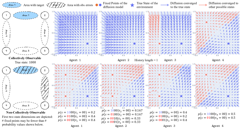
Figure 1. With minimal deep learning approximation errors, diffusion processes represent states consistent with local history $\tau_{i}$ (length=1 in this figure) as their attractors, provably equivalent to stable fixed points of the diffusion model $f_{\theta}\IfBlankTF{\tau_{i}}{}{({\tau_{i}}},\IfBlankTF{\cdot}{}{{\cdot}})$. Arrows point to diffusion model outputs $y^{\prime}=f_{\theta}\IfBlankTF{\tau_{i}}{}{({\tau_{i}}},\IfBlankTF{y}{}{{y}})$ from input noisy states $y$. The first two dimensions of $y^{\prime}$ and $y$ are shown. Top row: In collectively observable (CO) Dec-POMDPs, a unique fixed point is shared by all agents, which is also the true state. Bottom row: In non-CO Dec-POMDPs, shared fixed points are all states consistent with joint history $\bm{\tau}$, and diffusion models reproduce the posterior state distribution $p(s|\tau_{i})$ under appropriate distributions of input noisy states.

As shown in Sec. A.1, adapting the derivation from Robbins (1992); Miyasawa et al. (1961); Kadkhodaie et al. (2023), the optimal diffusion model yields the expected state given the noisy input $y$:

$$f^{\star}\IfBlankTF{\tau_{i}}{}{({\tau_{i}}},\IfBlankTF{y}{}{{y}})=\mathbb{E}_{s}\left[s\big{|}y,\tau_{i}\right],$$ (1)

which is related to the conditional scores by

$$\nabla\log p_{\sigma}(y|\tau_{i})=\frac{1}{\sigma^{2}}\left(\mathbb{E}_{s}\left[s\big{|}y,\tau_{i}\right]-y\right).$$ (2)

The approximation of this density family $\{p_{\sigma}(y|\tau_{i})\ |\ \sigma>0\}$ defines a model $p_{\theta}\IfBlankTF{s}{}{({s}}|\IfBlankTF{\tau_{i}}{}{{\tau_{i}}})$ of the posterior distribution of clean states (Kadkhodaie et al. (2023), Eq. 5), analogous to the temporal evolution of a diffusion process.

Posterior state distribution and discrete-time flow.  We are concerned with the estimated states and their distribution after applying the diffusion model repeatedly. We first define the flow induced by the diffusion model.

Definition 0 (Flow induced by the diffusion model).

A discrete-time flow $\phi\IfBlankTF{\ell}{}{{}_{\ell}}\IfBlankTF{}{}{}\IfBlankTF{\tau_{i}}{}{(\tau_{i}}\IfBlankTF{\theta}{}{,\theta}\IfBlankTF{\tau_{i}}{}{)}:\mathbb{N}\times\mathbb{R}^{|s|}\rightarrow\mathbb{R}^{|s|}$ conditioned on local history $\tau_{i}$ and diffusion model parameters $\theta$ is defined by

$$\phi\IfBlankTF{\ell}{}{{}_{\ell}}\IfBlankTF{}{}{}\IfBlankTF{\tau_{i}}{}{(\tau_{i}}\IfBlankTF{\theta}{}{,\theta}\IfBlankTF{\tau_{i}}{}{)}(y)=f\left(\tau_{i},\phi\IfBlankTF{\ell-1}{}{{}_{\ell-1}}\IfBlankTF{}{}{}\IfBlankTF{\tau_{i}}{}{(\tau_{i}}\IfBlankTF{\theta}{}{,\theta}\IfBlankTF{\tau_{i}}{}{)}(y)\right)$$ (3)

with the initial condition $\phi\IfBlankTF{0}{}{{}_{0}}\IfBlankTF{}{}{}\IfBlankTF{\tau_{i}}{}{(\tau_{i}}\IfBlankTF{\theta}{}{,\theta}\IfBlankTF{\tau_{i}}{}{)}(y)=y$.

Intuitively, a flow provides a denoised state after applying the diffusion model $\ell$ times, transporting the noisy state $y$ to an estimated state $y^{(\ell)}=\phi\IfBlankTF{\ell}{}{{}_{\ell}}\IfBlankTF{}{}{}\IfBlankTF{\tau_{i}}{}{(\tau_{i}}\IfBlankTF{\theta}{}{,\theta}\IfBlankTF{\tau_{i}}{}{)}(y)$. The distribution of these denoised states is given by the push-forward equation defined as follows.

Definition 0 (Push-forward equation).

The distribution of estimated states after applying the diffusion model for $\ell$ times is

$$p_{\ell}=[\phi\IfBlankTF{\ell}{}{{}_{\ell}}\IfBlankTF{}{}{}\IfBlankTF{\tau_{i}}{}{(\tau_{i}}\IfBlankTF{\theta}{}{,\theta}\IfBlankTF{\tau_{i}}{}{)}]_{*}p_{0},$$ (4)

where $p_{0}$ is the prior distribution of states, and the push-forward operator $*$ is defined by $[\phi\IfBlankTF{\ell}{}{{}_{\ell}}\IfBlankTF{}{}{}\IfBlankTF{\tau_{i}}{}{(\tau_{i}}\IfBlankTF{\theta}{}{,\theta}\IfBlankTF{\tau_{i}}{}{)}]_{*}p_{0}(y)=p_{0}(\phi_{\ell}^{-1}(y))\det\left[\partial\phi_{\ell}^{-1}/\partial y\right].$

In this way, the estimated posterior state distribution given by the diffusion model is

$$p_{\theta}\IfBlankTF{s}{}{({s}}|\IfBlankTF{\tau_{i}}{}{{\tau_{i}}})=[\phi\IfBlankTF{\ell\rightarrow\infty}{}{{}_{\ell\rightarrow\infty}}\IfBlankTF{}{}{}\IfBlankTF{\tau_{i}}{}{(\tau_{i}}\IfBlankTF{\theta}{}{,\theta}\IfBlankTF{\tau_{i}}{}{)}]_{*}p_{0}(s).$$ (5)

According to Definition 3, this distribution depends on the Jacobian $\partial\phi_{\ell}^{-1}/\partial y=(\partial\phi_{\ell}/\partial y)^{-1}$ Lipman et al. (2022). As $\phi_{\ell}$ is dependent on $f_{\theta}\IfBlankTF{\tau_{i}}{}{({\tau_{i}}},\IfBlankTF{y}{}{{y}})$, our analysis would heavily utilize the diffusion network Jacobian

$$J\IfBlankTF{f}{}{{}_{f}}\IfBlankTF{}{}{}\IfBlankTF{y}{}{(y}\IfBlankTF{\tau_{i}}{}{|\tau_{i}}\IfBlankTF{y}{}{)}=\nabla_{y}f_{\theta}\IfBlankTF{\tau_{i}}{}{({\tau_{i}}},\IfBlankTF{y}{}{{y}})=\left.\partial f/\partial y\right|_{(\tau_{i},y)}.$$ (6)

For simplicity, we assume the Jacobian is symmetric and non-negative, which is approximately true for the network Jacobian Mohan et al. (2020) and can be proved to hold for the optimal diffusion model Kadkhodaie et al. (2023). $J\IfBlankTF{f}{}{{}_{f}}\IfBlankTF{}{}{}\IfBlankTF{y}{}{(y}\IfBlankTF{\tau_{i}}{}{|\tau_{i}}\IfBlankTF{y}{}{)}$ has eigenvalues $\lambda\IfBlankTF{k}{}{{}_{k}}\IfBlankTF{}{}{}\IfBlankTF{y}{}{(y}\IfBlankTF{\tau_{i}}{}{|\tau_{i}}\IfBlankTF{y}{}{)}$ and eigenvectors $e\IfBlankTF{k}{}{{}_{k}}\IfBlankTF{}{}{}\IfBlankTF{y}{}{(y}\IfBlankTF{\tau_{i}}{}{|\tau_{i}}\IfBlankTF{y}{}{)},k\in[|s|]$. Dependencies on $y$ and $\tau_{i}$ will be omitted in these notations when they are unambiguous within the given context. An important property we use in this paper is the Jacobian rank, defined as the rank of the matrix $J\IfBlankTF{}{}{}\IfBlankTF{+}{}{{}^{+}}\IfBlankTF{y}{}{(y}\IfBlankTF{\tau}{}{|\tau}\IfBlankTF{y}{}{)}=\left(I-\frac{\partial f}{\partial y}(\tau,y)\right)^{-1}\frac{\partial f}{\partial\tau}(\tau,y).$

3. States As Shared Fixed Points

We now present our findings on how diffusion models represent the one-to-many mapping from histories to states. We first consider the case with minimal influence of deep learning approximation errors in this section, and study more complex scenarios in Sec. 4.

3.1. Example

We start with a didactic example. Sensor networks are a classic problem in the multi-agent literature Modi et al. (2001); Nair et al. (2005); Zhang and Lesser (2011) inspired by real-world challenges Lesser et al. (2003). The environment consists of multiple sensor agents and moving targets. Each sensor agent can scan at most one nearby area per timestep, and two agents must scan an area simultaneously to track targets. Since we are studying the case with minimal influence of deep learning approximation errors in this section, we use a small sensor network with 2$\times$2 sensor agents (1^st column of Fig. 1, with each sensor represented by a circle) and 1 target. There are four possible states, with each state $s\in\mathbb{R}^{4}$ being a one-hot vector indicating the target’s true location.

Collectively observable Dec-POMDPs. The first row of Fig. 1 illustrates a collectively observable Dec-POMDP Pynadath and Tambe (2002). Each agent’s observation $o\in\mathbb{R}^{2}$ includes a separate dimension for each nearby area, with a value 1 if the target is present and 0 otherwise. In this example, the target is in $\mathtt{Area\ 1}$. The right side plots changes in the first two state dimensions during diffusion. Each arrow starts from a possible noisy state, which, together with local history, is the input to the diffusion network. The network outputs a denoised state, marking the endpoint of the arrow. $\mathtt{Agent\ 3}$ and $\mathtt{4}$ have uncertainty because they cannot observe the target in their nearby areas. This uncertainty is reflected in the diffusion vector fields. Conditioned on their histories (length=1), the diffusion model has two fixed points, each representing a possible state. For example, $\mathtt{Agent\ 3}$ cannot distinguish whether the target is in $\mathtt{Area\ 1}$ or $\mathtt{Area\ 4}$; correspondingly, the diffusion model has two attractors $y=(1,0,0,0)$ and $(0,0,0,1)$. Moreover, we observe that the diffusion model has an equal probability of converging to these two fixed points, matching the true posterior state distribution given the history. $\mathtt{Agent\ 1}$ and $\mathtt{2}$ know the true state because they observe the target. Correspondingly, there is only one fixed point $(1,0,0,0)$ given their history. More importantly, we note that the only common fixed point shared by all agents is the true state $(1,0,0,0)$.

Non-collectively observable Dec-POMDPs.  The second row of Fig. 1 illustrates a non-collectively observable Dec-POMDPs. The agent observation is the same as before, but when the target appears in $\mathtt{Area\ 1}$ or $\mathtt{Area\ 2}$, nearby sensors have a 50% chance of failing to observe it. For example, when the true state is $(1,0,0,0)$, the observation of $\mathtt{Agent\ 1}$ can be either $(1,0)$ or $(0,0)$ with equal probability. This environment is non-collectively observable because it is possible for all agents to receive an observation $(0,0)$, in which case even aggregating all local information does not reveal the target’s location, as shown in Fig. 1. We observe a significant difference from the first row: now there are multiple shared fixed points: $(1,0,0,0)$ and $(0,1,0,0)$. This reflects the best inference the agents can achieve: from $\mathtt{Agent\ 3}$ and $\mathtt{Agent\ 4}$’s observation, they know for sure that the target is not in $\mathtt{Area\ 3}$ or $\mathtt{Area\ 4}$. However, the aggregated local information cannot distinguish whether the target is in $\mathtt{Area\ 1}$ or $\mathtt{Area\ 2}$.

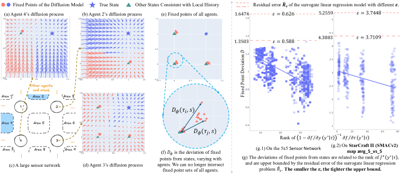
Figure 2. Deep learning approximation errors cause fixed points to deviate from true states. Deviation norms are related to the Jacobian rank and can be upper bounded by a surrogate linear model. (a,b,d) In the 5$\times$5 sensor network (with a zoomed-in view in (c)), we show changes in state dimensions corresponding to $\mathtt{Area2}$ and $\mathtt{4}$ during diffusion. (e,f) The impact of these deviations becomes evident when fixed points of all agents are displayed together in a single panel: the true state can no longer be determined by intersecting fixed point sets of all agents, as it is possible that $\cap_{i}\mathcal{F}\IfBlankTF{\phi}{}{{}_{\phi}}\IfBlankTF{}{}{}\IfBlankTF{\tau_{i}}{}{(\tau_{i}}\IfBlankTF{\tau_{i}}{}{)}=\varnothing$. (g) Empirical evidence from SMACv2 and the 5$\times$5 sensor network shows that deviation norms negatively correlate to Jacobian ranks and are tightly upper bounded by optimal residual errors of the surrogate linear model.

3.2. Infer State Locally: Stable Fixed Points

Although simple, the sensor network example encapsulates our findings which will be discussed in this section. Our first finding pertains to how diffusion models represent states, i.e., how each agent infers states based on its own history. We begin by showing that these individual diffusion processes converge.

theoremconverge[Converged Diffusion] When there are no approximation errors, repeatedly applying the diffusion model $f_{\theta}\IfBlankTF{\tau_{i}}{}{({\tau_{i}}},\IfBlankTF{y}{}{{y}})$ converges to a state $s$ that is consistent with $\tau_{i}$ and has a dominate posterior probability given the diffusion input $y$

$$\phi\IfBlankTF{\infty}{}{{}_{\infty}}\IfBlankTF{}{}{}\IfBlankTF{\tau_{i}}{}{(\tau_{i}}\IfBlankTF{\theta}{}{,\theta}\IfBlankTF{\tau_{i}}{}{)}(y)=s=\operatorname*{arg\,max}_{s\in S_{G}(\tau_{i})}p(s|y,\tau_{i}).$$ (7)

Sec. 3.2 is proved in Sec. A.2 and formally underpins the observation in Fig. 1 that diffusion models converge to states consistent with the local history. Based on this, we give the sufficient and necessary conditions of how the diffusion model represents states.

theoremrepr[State Representation] The diffusion model $f_{\theta}\IfBlankTF{\tau_{i}}{}{({\tau_{i}}},\IfBlankTF{\cdot}{}{{\cdot}})$ represents states consistent with $\tau_{i}$ by the attractors of its flow:

$$\hat{S}_{G}(\tau_{i})=\left\{y^{*}\mid[\phi\IfBlankTF{\infty}{}{{}_{\infty}}\IfBlankTF{}{}{}\IfBlankTF{\tau_{i}}{}{(\tau_{i}}\IfBlankTF{\theta}{}{,\theta}\IfBlankTF{\tau_{i}}{}{)}]_{*}p_{0}(y^{*})>0\right\},$$ (8)

which are equivalent to the stable fixed points $\mathcal{F}\IfBlankTF{\phi}{}{{}_{\phi}}\IfBlankTF{}{}{}\IfBlankTF{\tau_{i}}{}{(\tau_{i}}\IfBlankTF{\tau_{i}}{}{)}$ of $f_{\theta}\IfBlankTF{\tau_{i}}{}{({\tau_{i}}},\IfBlankTF{\cdot}{}{{\cdot}})$,

$$\mathcal{F}\IfBlankTF{\phi}{}{{}_{\phi}}\IfBlankTF{}{}{}\IfBlankTF{\tau_{i}}{}{(\tau_{i}}\IfBlankTF{\tau_{i}}{}{)}=\{y^{*}\mid y^{*}=f_{\theta}\IfBlankTF{\tau_{i}}{}{({\tau_{i}}},\IfBlankTF{y^{*}}{}{{y^{*}}}),|\lambda\IfBlankTF{\max}{}{{}_{\max}}\IfBlankTF{}{}{}\IfBlankTF{y^{*}}{}{(y^{*}}\IfBlankTF{\tau_{i}}{}{|\tau_{i}}\IfBlankTF{y^{*}}{}{)}|<1\}.$$ (9)

Here, $\lambda\IfBlankTF{\max}{}{{}_{\max}}\IfBlankTF{}{}{}\IfBlankTF{y^{*}}{}{(y^{*}}\IfBlankTF{\tau_{i}}{}{|\tau_{i}}\IfBlankTF{y^{*}}{}{)}$ is the largest eigenvalue of the Jacobian $J\IfBlankTF{f}{}{{}_{f}}\IfBlankTF{}{}{}\IfBlankTF{y^{*}}{}{(y^{*}}\IfBlankTF{\tau_{i}}{}{|\tau_{i}}\IfBlankTF{y^{*}}{}{)}$. A detailed proof is in Sec. A.2. Sec. 3.2 shows $\mathcal{F}\IfBlankTF{\phi}{}{{}_{\phi}}\IfBlankTF{}{}{}\IfBlankTF{\tau_{i}}{}{(\tau_{i}}\IfBlankTF{\tau_{i}}{}{)}=\hat{S}_{G}(\tau_{i})$, and when there is no approximation errors, the stable fixed points are exactly the states consistent with $\tau_{i}$: $\mathcal{F}\IfBlankTF{\phi}{}{{}_{\phi}}\IfBlankTF{}{}{}\IfBlankTF{\tau_{i}}{}{(\tau_{i}}\IfBlankTF{\tau_{i}}{}{)}=S_{G}(\tau_{i}).$

3.3. Infer State Globally: Shared Fixed Points

Secs. 3.2 and 3.2 show how individual diffusion models $f_{\theta}\IfBlankTF{\tau_{i}}{}{({\tau_{i}}},\IfBlankTF{\cdot}{}{{\cdot}})$ represent the inference of agent $i$ about states. In the simplest scenario described in the finding below, this local inference suffices to determine the true global state.

Finding 1.

If the individual diffusion model $f_{\theta}\IfBlankTF{\tau_{i}}{}{({\tau_{i}}},\IfBlankTF{y}{}{{y}})$ has only one stable fixed point $y^{*}$, agent $i$ is able to infer that $s=y^{*}$.

A unique fixed point implies that only one state is consistent with $\tau_{i}$. Therefore, agent $i$ can unambiguously determine the global state, eliminating the need for communication with others.

We focus primarily on more complex scenarios where agents are uncertain about the state, i.e., individual diffusion models have multiple fixed points. We first show that, if the Dec-POMDP is collectively observable, this uncertainty can be effectively resolved.

theoremRzeroCO Without approximation errors, in collectively observable Dec-POMDPs, the intersection of the fixed point sets of all agents is the true state: $\cap_{i}\mathcal{F}\IfBlankTF{\phi}{}{{}_{\phi}}\IfBlankTF{}{}{}\IfBlankTF{\tau_{i}}{}{(\tau_{i}}\IfBlankTF{\tau_{i}}{}{)}=\{s\}.$

Conversely, non-collectively observable Dec-POMDPs are more complicated, as agents are collectively unable to uniquely determine the state. However, we can still show that diffusion models identify all states consistent with the joint history and can reproduce the posterior distribution over these states.

theoremRzeroNonCO Without approximation errors, in non-collectively observable Dec-POMDPs, the intersection of fixed point sets is all states consistent with joint history:

$$\cap_{i}\mathcal{F}\IfBlankTF{\phi}{}{{}_{\phi}}\IfBlankTF{}{}{}\IfBlankTF{\tau_{i}}{}{(\tau_{i}}\IfBlankTF{\tau_{i}}{}{)}=\{s\mid p(s|\bm{\tau})>0\}.$$ (10)

The optimal posterior distribution $p(s|\bm{\tau})$ can be recovered with appropriate prior distributions $p(y)$ of initial noisy states $y$.

1 and 1 (proved in Sec. A.3) establish a communication protocol–agents share their local fixed points when necessary to maximally resolve uncertainty regarding the true state.

4. Deviated Fixed Points

We now consider the influence of deep learning approximation errors. Specifically, (1) We find that the major impact of these errors is that fixed points deviate from states (Fig. 2(a-f)). (2) Theoretically, we identify Jacobian ranks of diffusion models as the primary factor driving this deviation (Definition 4). Empirical results (Fig. 2(g)) support this finding and pinpoint practical design choices that influence Jacobian ranks (Fig. 3). (3) Inspired by the low-rank property, we construct a surrogate linear regression model (3) to bound the deviation (4). (4) This deviation bound helps prove the convergence of a novel composite diffusion process (Sec. 5).

4.1. Example

We begin with a concrete example that expands the sensor network to include $5\times 5$ agents and 2 targets, with each sensor configured to scan 4 nearby areas. Fig. 2(c) zooms in on the section of the map containing two targets. For a fair comparison against the example in the previous section, we keep the network architecture and training agenda unchanged (details in Appx. B).

In Fig. 2(a,b,d), we show the discrete-time flow induced by the diffusion model in this task. The increased size puts an extra burden on the diffusion model. For example, in Fig. 2(d), the diffusion model of $\mathtt{Agent\ 3}$ converges to four fixed points (blue and red circles), which are not strictly overlapped with possible states (blue star and green triangles), indicating that fixed points deviate from clean states. For better visualization, in Fig. 2(f), we put the fixed points of all agents together and zoom in on the fixed points around (0,0). It shows that diffusion models of different agents exhibit distinct fixed points with varied deviations. In this way, it is no longer practical to calculate the intersection of agents’ fixed point sets to obtain the true state, as the intersection would be empty.

4.2. Jacobian Rank and Surrogate Linear Model

Empirical Observations.  To understand why the diffusion model can no longer represent the consistent states $S_{G}(\tau_{i})$ accurately, we take a closer look at the fixed points learned by the diffusion model in the $5\times 5$ sensor network (Fig. 2(c)) and the $\mathtt{zerg\_5\_vs\_5}$ map from the complex, highly stochastic SMACv2 benchmark (Ellis et al., 2023). Specifically, we look at the Jacobian rank at each fixed point of individual agents.

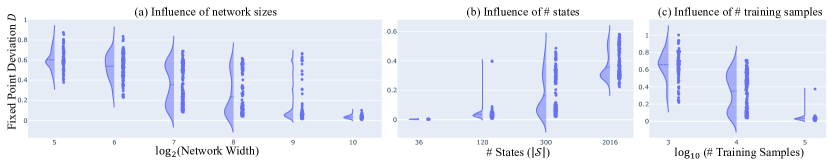
Figure 3. Practical factors contributing to low Jacobian ranks (which correlate negatively with deviations of fixed points from true states) include narrow network architectures, large state space sizes, and small numbers of training samples. In each panel, a blue point represents the deviation of a fixed point, and distributions of these deviations are displayed on the left.

Fig. 2(g) shows the relationship between fixed points’ Jacobian ranks and their deviations from states (in $\ell_{2}$ norm). A clear negative correlation is observed between these two variables, i.e., fixed points with lower Jacobian ranks are more likely to exhibit large deviations from true states.

Theoretical Understanding.   We now formally analyze the underlying reason for this negative correlation and thereby show why diffusion models might not be able to represent all states accurately. We first define the deviation of fixed points from states as follows.

Definition 0 (Deviation of fixed points from states).

We define the error between a true state $s$ and its corresponding fixed point by

$$D\IfBlankTF{\phi}{}{{}_{\phi}}\IfBlankTF{}{}{}\IfBlankTF{\tau_{i}}{}{(\tau_{i}}\IfBlankTF{s}{}{,s}\IfBlankTF{\tau_{i}}{}{)}=s-\phi\IfBlankTF{\infty}{}{{}_{\infty}}\IfBlankTF{}{}{}\IfBlankTF{\tau_{i}}{}{(\tau_{i}}\IfBlankTF{\theta}{}{,\theta}\IfBlankTF{\tau_{i}}{}{)}(s).$$ (11)

Here, $\phi\IfBlankTF{\infty}{}{{}_{\infty}}\IfBlankTF{}{}{}\IfBlankTF{\tau_{i}}{}{(\tau_{i}}\IfBlankTF{\theta}{}{,\theta}\IfBlankTF{\tau_{i}}{}{)}(s)$ is the attractor to which the iterative diffusion process conditioned on $\tau_{i}$ converges when initialized from state $s$.

Our analysis begins with the following theorem that characterizes the influence of $\tau$ on the fixed points, i.e., how the fixed point changes when $\tau$ changes.

theoremlr Let $y^{*}\in\mathcal{F}\IfBlankTF{\phi}{}{{}_{\phi}}\IfBlankTF{}{}{}\IfBlankTF{\tau}{}{(\tau}\IfBlankTF{\tau}{}{)}$ be a fixed point corresponding to history $\tau$. When $\tau$ changes to $\tau^{\prime}=\tau+\Delta\tau$, the fixed point shifts to $y^{*}{}^{\prime}=y^{*}+\Delta y^{*}$. If the changes in Jacobian satisfies $\|J\IfBlankTF{f}{}{{}_{f}}\IfBlankTF{}{}{}\IfBlankTF{\tau^{\prime},y^{*}{}^{\prime}}{}{(\tau^{\prime},y^{*}{}^{\prime}}\IfBlankTF{\tau^{\prime},y^{*}{}^{\prime}}{}{)}-J\IfBlankTF{f}{}{{}_{f}}\IfBlankTF{}{}{}\IfBlankTF{\tau,y^{*}}{}{(\tau,y^{*}}\IfBlankTF{\tau,y^{*}}{}{)}\|_{F}<\epsilon$ for a small $\epsilon$, we have

$$\Delta y^{*}\approx\left(I-\frac{\partial f}{\partial y}(\tau,y^{*})\right)^{-1}\frac{\partial f}{\partial\tau}(\tau,y^{*})\Delta\tau.$$ (12)

The approximation error in Eq. 12 is bounded by $\left\|\mathtt{Err}(\Delta y^{*})\right\|\leq\frac{M\epsilon^{2}}{2(1-\lambda\IfBlankTF{\max}{}{{}_{\max}}\IfBlankTF{}{}{})m^{2}},$ where $\lambda\IfBlankTF{\max}{}{{}_{\max}}\IfBlankTF{}{}{}$ is the largest Jacobian eigenvalue at $y^{*}$, and $M,m$ is the upper/lower bound on the norm of Hessian. Due to its $O(\epsilon^{2})$ magnitude, this error is negligible when $\epsilon$ is small.

Finding 2.

The major takeaway of Definition 4 emerges from Eq. 12. This equation implies that the diffusion model behaves like a (locally) linear model $\Delta y^{*}\approx J\IfBlankTF{}{}{}\IfBlankTF{+}{}{{}^{+}}\IfBlankTF{y^{*}}{}{(y^{*}}\IfBlankTF{\tau}{}{|\tau}\IfBlankTF{y^{*}}{}{)}\Delta\tau$ with weights

$$J\IfBlankTF{}{}{}\IfBlankTF{+}{}{{}^{+}}\IfBlankTF{y^{*}}{}{(y^{*}}\IfBlankTF{\tau}{}{|\tau}\IfBlankTF{y^{*}}{}{)}=\left(I-\frac{\partial f}{\partial y}(\tau,y^{*})\right)^{-1}\frac{\partial f}{\partial\tau}(\tau,y^{*})$$ (13)

to approximate the shifts of fixed points when local history changes.

We expand Eq. 12 in the special case where the diffusion model is a fully-connected network in 2. corollarylrfc If $f_{\theta}\IfBlankTF{\tau}{}{({\tau}},\IfBlankTF{y}{}{{y}})=g(\sigma(W_{\tau}\tau+W_{y}y+b))$ is a fully connected network. $\sigma(\cdot)$ is an element-wise activation function and $g(\cdot)$ represents the subsequent fully connected layers, which may introduce additional non-linearities following the first layer, we have

$$\Delta y^{*}\approx U(I-\Lambda)^{-1}\Lambda U\IfBlankTF{}{}{}\IfBlankTF{\top}{}{{}^{\top}}W_{y}^{+}W_{\tau}\Delta\tau,$$ (14)

where $U\Lambda U\IfBlankTF{}{}{}\IfBlankTF{\top}{}{{}^{\top}}$ is Jacobian eigen-decomposition of $f_{\theta}$ at $y^{*}$, $W_{y}^{+}$ is Moore–Penrose inverse $W_{y}^{+}=W_{y}^{\top}(W_{y}W_{y}^{\top})^{-1}$. Proved in Sec. A.4, 2 examines a specific network architecture, while the other analyses in this paper are applicable to any diffusion network architectures.

Based on Definition 4, we use proof by contradiction to show that diffusion models might not have enough capacity to represent all states accurately. We start with a local history $\tau$ and a consistent state $s$, assuming that the diffusion model conditioned on $\tau$ has enough capacity to exactly represent $s$ by a fixed point $y^{*}$. We then consider other histories near $\tau$: $\mathcal{T}_{\epsilon}=\{\tau^{\prime}\mid\|J\IfBlankTF{f}{}{{}_{f}}\IfBlankTF{}{}{}\IfBlankTF{\tau^{\prime},y^{*}{}^{\prime}}{}{(\tau^{\prime},y^{*}{}^{\prime}}\IfBlankTF{\tau^{\prime},y^{*}{}^{\prime}}{}{)}-J\IfBlankTF{f}{}{{}_{f}}\IfBlankTF{}{}{}\IfBlankTF{\tau,y^{*}}{}{(\tau,y^{*}}\IfBlankTF{\tau,y^{*}}{}{)}\|_{F}\leq\epsilon\}$. Each $\tau^{\prime}\in\mathcal{T}_{\epsilon}$ has a corresponding consistent state $s^{\prime}$ and a fixed point $y^{*}{}^{\prime}$. Due to 2, the diffusion model is trained to (locally) solve the following optimization problem.

Definition 0 (Surrogate Local Linear Regression Model).

For a local history $\tau$ and a consistent state $s$, let $\mathcal{M}\IfBlankTF{\epsilon}{}{{}_{\epsilon}}\IfBlankTF{}{}{}\IfBlankTF{}{}{(}\IfBlankTF{}{}{,}\IfBlankTF{}{}{)}\subset\mathcal{D}$ be a sample set containing $(\tau^{\prime},s^{\prime})$ in the training dataset $\mathcal{D}$ satisfying $\|J\IfBlankTF{f}{}{{}_{f}}\IfBlankTF{}{}{}\IfBlankTF{\tau,y^{*}}{}{(\tau,y^{*}}\IfBlankTF{\tau,y^{*}}{}{)}-J\IfBlankTF{f}{}{{}_{f}}\IfBlankTF{}{}{}\IfBlankTF{\tau^{\prime},y^{*}{}^{\prime}}{}{(\tau^{\prime},y^{*}{}^{\prime}}\IfBlankTF{\tau^{\prime},y^{*}{}^{\prime}}{}{)}\|_{F}$ $\leq\epsilon$. The surrogate linear regression problem is:

$$\mathcal{R}_{\epsilon}:\ \ \ \operatorname*{arg\,min}_{W\in{\mathbb{R}}^{|s|\times|\tau|}}\sum_{(\tau^{\prime},s^{\prime})\in\mathcal{M}\IfBlankTF{\epsilon}{}{{}_{\epsilon}}\IfBlankTF{}{}{}\IfBlankTF{}{}{(}\IfBlankTF{}{}{,}\IfBlankTF{}{}{)}}\|W\Delta\tau-\Delta s\|^{2},$$ (15)

where $\Delta\tau=\tau-\tau^{\prime}$, $\Delta s=s-s^{\prime}$. The residual error of the optimal solution to $\mathcal{R}_{\epsilon}$ is $\hat{R}_{\epsilon}$. The number of linearly independent $s^{\prime}$ in $\mathcal{M}\IfBlankTF{\epsilon}{}{{}_{\epsilon}}\IfBlankTF{}{}{}\IfBlankTF{}{}{(}\IfBlankTF{}{}{,}\IfBlankTF{}{}{)}$ is

$$r(\mathcal{M}\IfBlankTF{\epsilon}{}{{}_{\epsilon}}\IfBlankTF{}{}{}\IfBlankTF{}{}{(}\IfBlankTF{}{}{,}\IfBlankTF{}{}{)})=\dim\left(\text{span}\left\{s^{\prime}\mid(\tau^{\prime},s^{\prime})\in\mathcal{M}\IfBlankTF{\epsilon}{}{{}_{\epsilon}}\IfBlankTF{}{}{}\IfBlankTF{}{}{(}\IfBlankTF{}{}{,}\IfBlankTF{}{}{)}\right\}\right).$$ (16)

Intuitively, given $\Delta\tau$, the diffusion model learns its local Jacobian $J\IfBlankTF{}{}{}\IfBlankTF{+}{}{{}^{+}}\IfBlankTF{y^{*}}{}{(y^{*}}\IfBlankTF{\tau}{}{|\tau}\IfBlankTF{y^{*}}{}{)}$ to minimize the difference between $\Delta y^{*}$ and the groundtruth $\Delta s$. The surrogate $\mathcal{R}_{\epsilon}$ provides the best linear solution to this optimization problem. The question is whether the diffusion model, locally, has enough capacity to perform better than this solution.

Finding 3.

If the diffusion network $f_{\theta}$ is over-parameterized with the maximum possible rank of $J\IfBlankTF{}{}{}\IfBlankTF{+}{}{{}^{+}}\IfBlankTF{y^{*}}{}{(y^{*}}\IfBlankTF{\tau}{}{|\tau}\IfBlankTF{y^{*}}{}{)}$ (Eq. 13) larger than the number of linearly independent state samples in the local regression problem $\mathcal{R}_{\epsilon}$:

$$\operatorname{rank}(J\IfBlankTF{}{}{}\IfBlankTF{+}{}{{}^{+}}\IfBlankTF{y^{*}}{}{(y^{*}}\IfBlankTF{\tau}{}{|\tau}\IfBlankTF{y^{*}}{}{)})\geq r(\mathcal{M}\IfBlankTF{\epsilon}{}{{}_{\epsilon}}\IfBlankTF{}{}{}\IfBlankTF{}{}{(}\IfBlankTF{}{}{,}\IfBlankTF{}{}{)}),$$ (17)

then the linear regression problem $\mathcal{R}_{\epsilon}$ is underdetermined, indicating that the diffusion model has enough capacity to represent the history-state mapping $S_{G}$.

On the other hand, if the diffusion model is under-parameterized, leaving $\operatorname{rank}(J\IfBlankTF{}{}{}\IfBlankTF{+}{}{{}^{+}}\IfBlankTF{y^{*}}{}{(y^{*}}\IfBlankTF{\tau}{}{|\tau}\IfBlankTF{y^{*}}{}{)})<r(\mathcal{M}\IfBlankTF{\epsilon}{}{{}_{\epsilon}}\IfBlankTF{}{}{}\IfBlankTF{}{}{(}\IfBlankTF{}{}{,}\IfBlankTF{}{}{)})$, then we have an over-determined regression problem that inevitably induces residual errors, leading to deviations of fixed points from states.

Evidence 3.1.

We empirically verify our findings in the 5$\times$5 sensor network. In Fig. 3-middle, we increase the problem size, so that $r(\mathcal{M}\IfBlankTF{\epsilon}{}{{}_{\epsilon}}\IfBlankTF{}{}{}\IfBlankTF{}{}{(}\IfBlankTF{}{}{,}\IfBlankTF{}{}{)})$ increases. With a fixed network size, we can see that $D\IfBlankTF{\phi}{}{{}_{\phi}}\IfBlankTF{}{}{}\IfBlankTF{\tau}{}{(\tau}\IfBlankTF{s}{}{,s}\IfBlankTF{\tau}{}{)}$ increases. We also find that increasing the network width can increase the rank of $J\IfBlankTF{}{}{}\IfBlankTF{+}{}{{}^{+}}\IfBlankTF{y^{*}}{}{(y^{*}}\IfBlankTF{\tau}{}{|\tau}\IfBlankTF{y^{*}}{}{)}$, and correspondingly decrease $D\IfBlankTF{\phi}{}{{}_{\phi}}$ as shown in Fig. 3-left. This is not trivial as the input dimension is fixed and is smaller than the network width, which means the rank of the $J\IfBlankTF{}{}{}\IfBlankTF{+}{}{{}^{+}}\IfBlankTF{y^{*}}{}{(y^{*}}\IfBlankTF{\tau}{}{|\tau}\IfBlankTF{y^{*}}{}{)}$ is actually upper bounded by the input dimension.

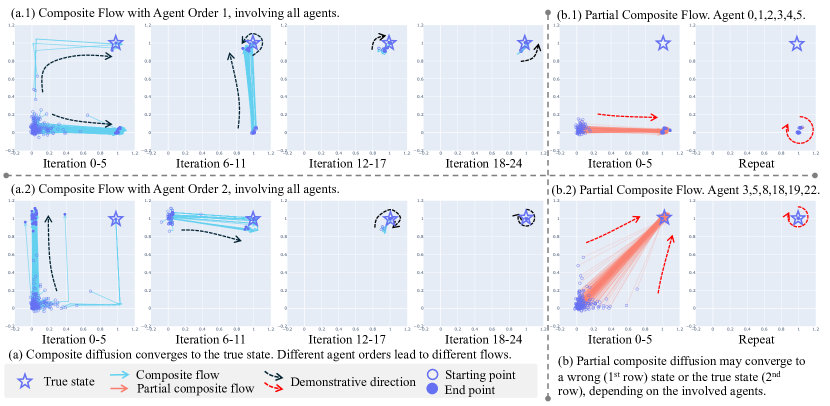
Figure 4. Evolution of denoised state distributions (first two dimensions) during composite diffusion processes, initialized with various noisy states, in the 5$\times$5 sensor network. Each panel shows the changes (from open circles to closed circles) over 6 diffusion iterations, with each iteration conditioned on the history of a single agent, e.g., in iteration 0-5, six agents in the corresponding order are involved. (a) Composite diffusion converges to the true state regardless of agent ordering. (b) Partial composite diffusion may converge to incorrect states depending on the participating agents.

4.3. Bounded Deviations

We now discuss how to bound the deviations $D\IfBlankTF{\phi}{}{{}_{\phi}}\IfBlankTF{}{}{}$.

Finding 4.

When $\epsilon$ is large, the expressivity of the diffusion model is more powerful than the surrogate regression model $\mathcal{R}_{\epsilon}$. This is because the diffusion network becomes more non-linear as the Jacobian changes significantly. In this case $\hat{R}_{\epsilon}$ is larger than $D\IfBlankTF{\phi}{}{{}_{\phi}}\IfBlankTF{}{}{}$, as $\hat{R}_{\epsilon}$ is the residual of a linear model, while $D\IfBlankTF{\phi}{}{{}_{\phi}}\IfBlankTF{}{}{}$ is the residual of a non-linear model. On the other hand, when we decrease $\epsilon$, The diffusion network is approaching linear and its capacity is getting close to the linear regression model, so $D\IfBlankTF{\phi}{}{{}_{\phi}}\IfBlankTF{}{}{}$ is getting close to $\hat{R}_{\epsilon}$.

We formally prove this finding in the following theorem. theoremfpdbound[Upper Bounded Deviation] Let $\mathcal{M}=\{(\tau_{(k)},s_{(k)})\}_{k=1}^{K_{1}}$. If there exist $\tau$ and $\tau^{\prime}$ in $\mathcal{M}$ where $\|J\IfBlankTF{f}{}{{}_{f}}\IfBlankTF{}{}{}\IfBlankTF{\tau^{\prime},y^{*}{}^{\prime}}{}{(\tau^{\prime},y^{*}{}^{\prime}}\IfBlankTF{\tau^{\prime},y^{*}{}^{\prime}}{}{)}-J\IfBlankTF{f}{}{{}_{f}}\IfBlankTF{}{}{}\IfBlankTF{\tau,y^{*}}{}{(\tau,y^{*}}\IfBlankTF{\tau,y^{*}}{}{)}\|_{F}>\epsilon$, then for $(\tau,s)\in\mathcal{M}$, we have

$$D\IfBlankTF{\phi}{}{{}_{\phi}}\IfBlankTF{}{}{}\IfBlankTF{\tau}{}{(\tau}\IfBlankTF{s}{}{,s}\IfBlankTF{\tau}{}{)}<\hat{R}(\mathcal{M})=\operatorname{Tr}(\Sigma_{s})-\operatorname{Tr}(\Sigma_{s\tau}\Sigma^{-1}_{\tau}\Sigma_{\tau s}).$$ (18)

Here $\Sigma_{s}=\mathbb{E}_{s\sim\mathcal{M}}[(s-\mathbb{E}[s])(s-\mathbb{E}[s])^{\top}]$, cross covariance $\Sigma_{s\tau}=\mathbb{E}_{(\tau,s)\sim\mathcal{M}}[(s-\mathbb{E}[s])(\tau-\mathbb{E}[\tau])^{\top}]$, and $\Sigma_{s\tau}=\Sigma_{\tau s}^{\top}$. $\hat{R}(\mathcal{M})$ is the residual error of the optimal linear regression model on $\mathcal{M}$.

Proved in Sec. A.5, 4 upper bound fixed point deviations by constructing a surrogate regression problem. By decreasing the $\epsilon$, we can tighten this upper bound, helping prove the convergence of our composite diffusion process in the next section.

Evidence 4.1.

We provide empirical evidence to support 4 and 4. The experiments are conducted on the 5$\times$5 sensor network (Fig. 2 (g.1)) and the $\mathtt{zerg\_5\_vs\_5}$ map (Fig. 2 (g.2)) from the complex, highly stochastic SMACv2 benchmark (Ellis et al., 2023). In (g.1), two dashed horizontal lines show the residual errors $\hat{R}_{\epsilon}$ of the surrogate linear regression model under two different $\epsilon$ values. When $\epsilon=0.626$, the linear regression model exhibits weaker representational capacity, with $\hat{R}_{0.626}=1.6474$ significantly larger than the deviations of the diffusion model. By contrast, when we decrease $\epsilon$ to 0.588, $\hat{R}_{0.588}$ provides a tight upper bound for the deviations. The case in SMACv2 is similar, indicating that the surrogate model effectively approximates the local behavior of the diffusion model.

5. Composite Diffusion

Table 1. True state estimation errors measured in PSNR. Higher PSNR values indicate lower errors. Individual diffusion exhibits a provable performance gap compared to composite diffusion.

Setting	Alg.	Network Width			# Training Samples			Obs. History Length			Obs. Sight Range		Tasks
		1024	4096	8192	10	100K	500K	1	5	10	5	9	Zerg	Terran	Protoss
Train	Individual	13.28	18.71	28.20	56.45	28.20	35.29	26.39	28.20	31.86	26.29	28.20	28.20	29.01	27.79
	Composite	15.98	22.18	30.77	56.77	30.77	36.39	27.88	30.77	33.13	27.92	30.77	30.77	30.68	30.20
Test	Individual	13.37	15.37	17.42	11.32	17.43	23.22	20.77	17.43	16.54	15.94	17.43	17.42	17.28	17.24
	Composite	16.07	18.49	20.40	12.38	20.40	25.49	23.54	20.40	18.94	17.90	20.40	20.40	18.59	20.08

As we discussed in Sec. 4, when fixed points deviate from clean states, it is impractical to obtain true states by intersecting all agents’ fixed points. Instead, we propose to use composite diffusion.

Definition 0 (Composite diffusion).

Let $[i_{1},i_{2},\cdots,i_{n}]\in\mathcal{P}([1,2,$ $\cdots,n])$ be a permutation of $[1,2,\cdots,n]$, where $n$ is the number of agents. The composite diffusion model conditioned on $\tau_{i_{1:n}}$ is

$$f_{\theta}\IfBlankTF{\tau_{i_{1:n}}}{}{({\tau_{i_{1:n}}}},\IfBlankTF{y}{}{{y}})=f_{\theta}(\tau_{i_{1}},f_{\theta}(\tau_{i_{2}}\cdots,f_{\theta}(\tau_{i_{n}},y))),$$ (25)

inducing a discrete-time composite flow $\phi\IfBlankTF{\ell}{}{{}_{\ell}}\IfBlankTF{}{}{}\IfBlankTF{\tau_{i_{1:n}}}{}{(\tau_{i_{1:n}}}\IfBlankTF{\theta}{}{,\theta}\IfBlankTF{\tau_{i_{1:n}}}{}{)}:{\mathbb{N}}\times{\mathbb{R}}^{|s|}\rightarrow{\mathbb{R}}^{|s|}$, $\phi\IfBlankTF{\ell}{}{{}_{\ell}}\IfBlankTF{}{}{}\IfBlankTF{\tau_{i_{1:n}}}{}{(\tau_{i_{1:n}}}\IfBlankTF{\theta}{}{,\theta}\IfBlankTF{\tau_{i_{1:n}}}{}{)}(y)=f\left(\tau_{i_{(\ell)_{n}}},\phi\IfBlankTF{\ell-1}{}{{}_{\ell-1}}\IfBlankTF{}{}{}\IfBlankTF{\tau_{i_{1:n}}}{}{(\tau_{i_{1:n}}}\IfBlankTF{\theta}{}{,\theta}\IfBlankTF{\tau_{i_{1:n}}}{}{)}(y)\right).$ $(\ell)_{n}=(\ell\mod n)$ is the remainder when $\ell$ is divided by $n$, and $\phi\IfBlankTF{0}{}{{}_{0}}\IfBlankTF{}{}{}\IfBlankTF{\tau_{i_{1:n}}}{}{(\tau_{i_{1:n}}}\IfBlankTF{\theta}{}{,\theta}\IfBlankTF{\tau_{i_{1:n}}}{}{)}(y)=y$.

A composite diffusion model iteratively applies individual diffusion models conditioned on each agent’s history. We then introduce an algorithm using composite diffusion to estimate true states.

5.1. Composite Diffusion Yields True States

Composite diffusion algorithm.  Our algorithm has two steps. Step 1 (Composite denoising): Sample a set of Gaussian noise $\{y^{(k,0)}\}_{k=0}^{K^{\prime}}$ from $\mathcal{N}(0,\sigma^{2}I)$. Apply composite diffusion to each $y^{(k,0)}$, resulting in a sequence of denoised states $(y^{(k,1)},\cdots,y^{(k,L)})$.

Step 2 (Condition check): Check whether the following two conditions hold. (1) For the last $n$ elements in the sequence, $y^{(k,\ell)},L-n<\ell\leq L$, the largest eigenvalue of the diffusion Jacobian at $y^{(k,\ell)}$ satisfies $|\lambda\IfBlankTF{\max}{}{{}_{\max}}\IfBlankTF{}{}{}|<1$. (2) Apply individual diffusion model conditioned on each agent’s history $\tau_{i}$ repeatedly to $y^{(k,L)}$ until converge, the change in $y^{(k,L)}$ should be smaller than $2D\IfBlankTF{\phi}{}{{}_{\phi}}$ (bounded by 4). These condition checks guarantee convergence to the true state as proven in the following theorem.

theoremalgoconv[Composite Diffusion Approaches True State] In collectively observable Dec-POMDPs, for a sequence $k$ that meets the conditions in Step 2, the composite diffusion algorithm approaches the true global state $s$ with an upper error bound:

$$\|y^{(k,L)}-s\|\leq\max_{1\leq i\leq n}D_{\phi}(\tau_{i},s).$$ (26)

Specifically, composite diffusion converges to the convex hull of the fixed points of all agents near $s$. Let ${\mathcal{F}}_{s}=\{y_{1}^{*}(s),y_{2}^{*}(s),\cdots,y_{n}^{*}(s)\}$ be the fixed point set near state $s$, $y_{i}^{*}(s)=\phi\IfBlankTF{\infty}{}{{}_{\infty}}\IfBlankTF{}{}{}\IfBlankTF{\tau_{i}}{}{(\tau_{i}}\IfBlankTF{\theta}{}{,\theta}\IfBlankTF{\tau_{i}}{}{)}(s)$. We have

$$y^{(k,L)}\in Conv({\mathcal{F}}_{s}).$$ (27)

Here

$$Conv({\mathcal{F}}_{s}):=\{\sum_{y_{i}^{*}\in{\mathcal{F}}_{s}}\beta_{i}y_{i}^{*}|\beta_{i}\geq 0,\sum_{i}^{n}\beta_{i}=1\}$$ (28)

is ${\mathcal{F}}_{s}$’s convex hull.

corollaryalgoconvnon In non-collectively observable Dec-POMDPs, with sufficiently enough initial samples, the composite diffusion algorithm approaches every possible global state $s$ consistent with joint history $\tau_{i_{1:n}}$ with an upper error bound:

$$\exists y^{(0)},s.t.\ \|\phi\IfBlankTF{\infty}{}{{}_{\infty}}\IfBlankTF{}{}{}\IfBlankTF{\tau_{i_{1:n}}}{}{(\tau_{i_{1:n}}}\IfBlankTF{\theta}{}{,\theta}\IfBlankTF{\tau_{i_{1:n}}}{}{)}(y^{(0)})-s\|\leq\max_{1\leq i\leq n}D_{\phi}(\tau_{i},s).$$ (29)

Sec. 5.1 and Sec. 5.1 are proved in Sec. A.7. They highlight the advantages of composite diffusion summarized as follows.

Finding 5.

Unlike individual diffusion conditioned on the history of a single agent, composite diffusion can resolve the uncertainty when there are multiple fixed points. Moreover, even in the simple case with only one fixed point, composite diffusion is able to provide a better estimation of the true state compared to individual diffusion, as proved in the following theorem.

theoremaccucom When there is only one fixed point for the diffusion model conditioned on $\tau_{i},i\in[n]$, assume that the final iterate $y^{(L)}$ distribute uniformly, composite diffusion provides a more accurate global state estimation than individual diffusion.

$$\mathbb{E}_{y^{(L)}}[\|y^{(L)}-s\|]\leq\frac{1}{|{\mathcal{F}}_{s}|}\sum\nolimits_{y_{i}^{*}\in{\mathcal{F}}_{s}}\|y_{i}^{*}-s\|.$$ (30)

Evidence 5.1.

In Table 1, we systematically evaluate the performance of composite diffusion against individual diffusion in the popular SMACv2 benchmark (Ellis et al., 2023). Training data is collected by running MAPPO (Yu et al., 2022) (with details in Appx. B). The evaluation involves various factors that can influence the diffusion model, including network sizes, numbers of training samples, history lengths, observation sight ranges, and tasks. For a fair comparison, composite diffusion and individual diffusion adopt the same number of denoising steps.

Table 1 shows the accuracy of estimated states measured in PSNR. PSNR is a common metric for the quality of noisy information, calculated as $10\log_{10}(MAX_{I}^{2}/MSE)$. In our case, $MAX_{I}$ is a constant and $MSE$ is the $\ell_{2}$ distance between the predicted state and true clean state. Higher PSNR indicates a lower error. Table 1 demonstrates that composite diffusion achieves higher PSNR across all the testing scenario, which is in line with our analyses. This performance gap is provable (5) even when the individual diffusion adopts a more powerful network architectures like in (Xu et al., 2024).

5.2. Partial Composite Diffusion

Composite diffusion requires a communication chain in which each agent receives the output of the preceding agent’s diffusion process and sends its own diffusion output to the subsequent agent. These messages reside in $\mathbb{R}^{|s|}$. In very large systems, it is possible to trade off this communication overhead against the accuracy of state estimation by involving only a subset of agents in the composite diffusion process. We thereby define partial composite diffusion $f_{\theta}\IfBlankTF{\tau_{i_{1:k}}}{}{({\tau_{i_{1:k}}}},\IfBlankTF{\cdot}{}{{\cdot}})$ and partial composite flow $\phi\IfBlankTF{\ell}{}{{}_{\ell}}\IfBlankTF{}{}{}\IfBlankTF{\tau_{i_{1:k}}}{}{(\tau_{i_{1:k}}}\IfBlankTF{\theta}{}{,\theta}\IfBlankTF{\tau_{i_{1:k}}}{}{)}$, in which $k<n$ and $[i_{1},i_{2},\cdots,i_{k}]\in{\mathbb{P}}([j_{1},j_{2},\cdots,j_{k}])$ is any of the permutations of the sub-sequence $[j_{1},j_{2},\cdots,j_{k}]$, where $1\leq j_{1}<j_{2}<\cdots<j_{k}\leq n$. We can adapt the composite diffusion algorithm and prove its convergence in Sec. 5.2.

corollaryalgoconvpartial With sufficiently enough initial samples, the partial composite diffusion algorithm approaches every possible global state $s$ consistent with $\tau_{i_{1:k}},k<n$, with an upper error bound:

$$\exists y^{(0)},s.t.\|\phi\IfBlankTF{\infty}{}{{}_{\infty}}\IfBlankTF{}{}{}\IfBlankTF{\tau_{i_{1:k}}}{}{(\tau_{i_{1:k}}}\IfBlankTF{\theta}{}{,\theta}\IfBlankTF{\tau_{i_{1:k}}}{}{)}(y^{(0)})-s\|\leq\max_{1\leq t\leq k}D_{\phi}(\tau_{i_{t}},s).$$ (31)

Finding 6.

Composite diffusion $f_{\theta}\IfBlankTF{\tau_{i_{1:n}}}{}{({\tau_{i_{1:n}}}},\IfBlankTF{y}{}{{y}})$ converges to the true global state, while partial composite diffusion $f_{\theta}\IfBlankTF{\tau_{i_{1:k}}}{}{({\tau_{i_{1:k}}}},\IfBlankTF{y}{}{{y}}),k<n$ may converge to wrong states, depending on the agents that participate in the partial composite diffusion process.

Evidence 6.1.

Fig. 4 shows the evolution of denoised state distributions (focusing on the first two dimensions) during the (partial) composite diffusion process in the 5$\times$5 sensor network. Initial noisy states are sampled from $\mathcal{N}(0,I)$. Composite flows consistently discover the true state regardless of agent ordering. In contrast, a partial composite flow stabilizes at a state consistent with histories, and whether this state is the true state depends on the participating agents.

6. Closing Remarks

This paper provides the first rigorous understanding of how deep learning models and their approximation errors can impact agents’ handling of PO in Dec-POMDPs. We expect that this work can establish a general framework for addressing the challenges posed by PO across various multi-agent sub-fields. As an initial demonstration of these possibilities, Appx. C provides an example where integrating diffusion models with policy learning can further enhance the performance of MARL algorithms, such as MAPPO Yu et al. (2022).

Appendix A Mathematical Derivations

A.1. Miyasawa Relationships

A clear connection between the score function and the MMSE estimator for a signal corrupted by additive Gaussian noise was initially established in Miyasawa et al. (1961) and later extended in Raphan and Simoncelli (2011); Efron (2011). We provide a derivation for the case conditioned on local history.

$$\nabla\log p(y|\tau_{i}) =\int p(s|\tau_{i})p(y|s,\tau_{i})\nabla_{y}\log p(y|s,\tau_{i})ds\Big{/}p(y|\tau_{i})$$

$$=\int p(s|y,\tau_{i})\nabla_{y}\log p(y|s,\tau_{i})ds$$ (32)

$$=\mathbb{E}\left[\nabla_{y}\log p(y|s,\tau_{i})\big{|}y,\tau_{i}\right]$$ (33)

Since $y\sim\mathcal{N}(s,\sigma^{2}I)$, we know

$$\log p(y|s,\tau_{i})=-\frac{1}{2\sigma^{2}}\|y-s\|^{2}-\log\left(\sqrt{2\pi\sigma^{2}}\right),$$ (34)

$$\nabla_{y}\log p(y|s,\tau_{i})=-\frac{1}{\sigma^{2}}(y-s).$$ (35)

Therefore,

$$\nabla\log p(y|\tau_{i}) =\mathbb{E}\left[-\frac{1}{\sigma^{2}}(y-s)\big{|}y,\tau_{i}\right]$$ (36)

$$=\frac{1}{\sigma^{2}}\left(\mathbb{E}_{s}\left[s\big{|}y,\tau_{i}\right]-y\right).$$ (37)

The optimal diffusion model satisfies

$$f^{\star}\IfBlankTF{\tau_{i}}{}{({\tau_{i}}},\IfBlankTF{y}{}{{y}})=y+\sigma^{2}\nabla\log p(y|\tau_{i})=\mathbb{E}_{s}\left[s\big{|}y,\tau_{i}\right].$$ (38)

A.2. Converged Individual Diffusion Processes

We put the proofs of the following two theorems together. * *

Proof.

We have shown that the diffusion model is approximating the posterior distribution $\mathbb{E}\left[s\big{|}y,\tau_{i}\right]$. When there are no approximation errors, we have

$$f_{\theta}\IfBlankTF{\tau_{i}}{}{({\tau_{i}}},\IfBlankTF{y}{}{{y}})=\mathbb{E}\left[s\big{|}y,\tau_{i}\right]=\int_{s}s\cdot p(s|\tau_{i},y)ds,$$ (39)

where

$$p(s|\tau_{i},y)=\frac{p(y|s,\tau_{i})p(s|\tau_{i})}{\int_{s}p(y|s,\tau_{i})p(s|\tau_{i})ds}=\frac{w_{s}(y)}{\int_{s}w_{s}(y)ds}$$ (40)

and

$$w_{s}(y)=p(s|\tau_{i})\exp\left(-\frac{\|y-s\|^{2}}{2\sigma^{2}}\right)$$ (41)

We now try to express $f_{\theta}\IfBlankTF{\tau_{i}}{}{({\tau_{i}}},\IfBlankTF{y}{}{{y}})$ as a gradient ascent step. Define the function

$$L(y)=\log\left(\int_{s}w_{s}(y)ds\right).$$ (42)

Compute the gradient of $L(y)$

$$\nabla_{y}L(y) =\frac{1}{\int_{s}w_{s}(y)ds}\int_{s}w_{s}(y)\left(-\frac{(y-s)}{\sigma^{2}}\right)$$ (43)

$$=-\frac{1}{\sigma^{2}}\int_{s}(y-s)\cdot\frac{w_{s}(y)}{\int_{s}w_{s}(y)ds}ds$$ (44)

It follows that

$$\sigma^{2}\nabla_{y}L(y)=-\int_{s}(y-s)\cdot p(s|\tau_{i},y)ds$$ (45)

Rewriting $f_{\theta}\IfBlankTF{\tau_{i}}{}{({\tau_{i}}},\IfBlankTF{y}{}{{y}})$:

$$f_{\theta}\IfBlankTF{\tau_{i}}{}{({\tau_{i}}},\IfBlankTF{y}{}{{y}}) =\int_{s}s\cdot p(s|\tau_{i},y)ds$$ (46)

$$=y+\int_{s}(s-y)\cdot p(s|\tau_{i},y)ds$$ (47)

$$=y+\sigma^{2}\nabla_{y}L(y)$$ (48)

It is obvious that the update rule of repeatedly applying the diffusion model $y^{(k+1)}=f_{\theta}\IfBlankTF{\tau_{i}}{}{({\tau_{i}}},\IfBlankTF{y^{(k)}}{}{{y^{(k)}}}))$ is:

$$y^{(k+1)}=y^{(k)}+\sigma^{2}\nabla_{y}L(y^{(k)})$$ (49)

This is a gradient ascent step on the function $L(y)$ with a fixed step size $\sigma^{2}$.

The function $L(y)$ has the following properties:

(1) $L(y)$ is infinitely differentiable, as it is composed of exponential and logarithmic functions of smooth arguments. (2) Each term $w_{s}(y)$ is log-concave in $y$ because it contains the exponential of a negative quadratic form. Therefore, $L(y)$ is the logarithm of a sum of log-concave functions, which is itself log-concave. (3) When $\sigma$ is small, function $L(y)$ attains local maxima at $y=s$, since the terms $w_{s}(y)$ are maximized when $y=s$.

Under standard assumptions for gradient ascent on smooth, concave functions, the sequence $\{y_{k}\}$ converges to a critical point (local maximum) of $L(y)$.

The critical points of $L(y)$ occur where $\nabla_{y}L(y)=0$. Setting the gradient to zero:

$$\nabla_{y}L(y)=0\implies\int_{s}(y-s)\cdot p(s|\tau_{i},y)ds=0$$ (50)

This simplifies to:

$$y=\int_{s}s\cdot p(s|\tau_{i},y)ds=f_{\theta}\IfBlankTF{\tau_{i}}{}{({\tau_{i}}},\IfBlankTF{y}{}{{y}})$$ (51)

So, at critical points, $y=f_{\theta}\IfBlankTF{\tau_{i}}{}{({\tau_{i}}},\IfBlankTF{y}{}{{y}})$, meaning $y$ is a fixed point of the iteration.

We also note that, since each step is a gradient ascent, $L(y_{k+1})\geq L(y_{k})$. $L(y)$ is also bounded above because $\int_{s}w_{s}(y)$ is finite. By the monotone convergence theorem, $L(y_{k})$ converges to some finite value $L^{*}$, and the sequence cannot oscillate between different $s$ because $L(y_{k})$ strictly increases unless $y^{(k)}$ is already at a critical point.

We also note that the convergence is generally exponential near the maximum due to the negative definiteness of the Hessian at $y=s$.

When the noise level $\sigma$ is small, the limit point $y^{*}$ must be one of the $s$, as these are the only critical points where $\nabla_{y}L(y)=0$. Diffusion models are trained across all noise levels with $\sigma>0$. When small values of $\sigma$ influence the diffusion process near $s$, the points $s$ become the only fixed points of the diffusion model.

∎

A.3. Shared Fixed Points

*

Proof.

When the diffusion model is accurate, each agent includes the state $s$ within its fixed point set. We then demonstrate that the intersection of all agents’ fixed point sets contains at most one element. Suppose, for the sake of contradiction, that the agents share two distinct states as fixed points, that is: $\Large\cap_{i}\mathcal{F}\IfBlankTF{\phi}{}{{}_{\phi}}\IfBlankTF{}{}{}\IfBlankTF{\tau_{i}}{}{(\tau_{i}}\IfBlankTF{\tau_{i}}{}{)}=\{s,s^{\prime}\}$. Since the diffusion models are conditioned on $\tau_{i}$, this implies that each agent $i$ observes $\tau_{i}$ in both states $s$ and $s^{\prime}$. Consequently, every agent $i$ has identical history in states $s$ and $s^{\prime}$. However, if the Dec-POMDP is collectively observable, identical history for all agents would necessitate that $s=s^{\prime}$. This contradiction confirms that the intersection set contains at most one element. ∎

*

Proof.

We first prove that $\Large\cap_{i}\mathcal{F}\IfBlankTF{\phi}{}{{}_{\phi}}\IfBlankTF{}{}{}\IfBlankTF{\tau_{i}}{}{(\tau_{i}}\IfBlankTF{\tau_{i}}{}{)}=\{s\mid p(s|\bm{\tau})>0\}$. For each $s$ such that $p(s|\bm{\tau})>0$, we know that the global state could be $s$ when the joint history is $\bm{\tau}$. Therefore, $(\tau_{i},s)$ is in the training dataset for the diffusion model conditioned on each $\tau_{i}$. When there is no approximation errors, $s$ would be a fixed point of each diffusion model $f_{\theta}\IfBlankTF{\tau_{i}}{}{({\tau_{i}}},\IfBlankTF{\cdot}{}{{\cdot}})$. On the other hand, for each state $s$ that is a fixed point for all $\tau_{i}$, we know that the sample $(\tau_{i},s)$ is in the dataset used to train the diffusion model, indicating that $p(\tau_{i}|s)>0$ and thus $p(s|\bm{\tau})\propto p(\bm{\tau}|s)p(s)>0$.

We then look at the posterior probability of a state $p_{\theta}\IfBlankTF{s}{}{({s}}|\IfBlankTF{\tau_{i}}{}{{\tau_{i}}})$. In the diffusion model, the probability we will reach state $s$ with $f_{\theta}\IfBlankTF{\tau_{i}}{}{({\tau_{i}}},\IfBlankTF{\cdot}{}{{\cdot}})$ is

$$p_{\theta}\IfBlankTF{s}{}{({s}}|\IfBlankTF{\tau_{i}}{}{{\tau_{i}}})=\int_{y\in\mathcal{B}_{\phi}(s)}p(y)dy.$$ (52)

Here $\mathcal{B}_{\phi}(s)$ is the basin of attraction of state $s$. From the proof of Sec. 3.2, we know that

$$\mathcal{B}_{\phi}(s)=\{y\mid p(s)p(y|s)>p(s^{\prime})p(y|s^{\prime}),\forall s^{\prime}\neq s\}.$$ (53)

Starting from any point $y$ in $\mathcal{B}_{\phi}(s)$ and applying the diffusion model conditioned on $\tau_{i}$ will converge to $s$ when $\sigma$ is small.

Here and in the following proof, we abuse the notations and omit the dependence on $\tau_{i}$ as it is clear in the context.

Our goal is to bound the gap between the convergence probability to state $s$ and the prior $p(s)$:

$$\text{Gap}(s)=\left|P_{\text{converge}}(s)-p(s)\right|,$$

where

$$P_{\text{converge}}(s)=\int_{\mathcal{B}_{\phi}(s)}p(y)dy.$$

The convergence probability to state $s$ is:

$$P_{\text{converge}}(s)=\int_{\mathcal{B}_{\phi}(s)}p(y)dy=\int_{\mathcal{B}_{\phi}(s)}\sum_{s^{\prime}}p(s^{\prime})p(y|s^{\prime})dy.$$

This can be split into two parts: (1) Correct classification (from state $s$):

$$A(s)=\int_{\mathcal{B}_{\phi}(s)}p(y|s)dy,$$

which is the probability that $y$ sampled from $p(y|s)$ falls into $\mathcal{B}_{\phi}(s)$. (2) Misclassification (from other states $s^{\prime}\neq s$):

$$B(s,s^{\prime})=\int_{\mathcal{B}_{\phi}(s)}p(y|s^{\prime})dy,$$

which is the probability that $y$ sampled from $p(y|s^{\prime})$ is incorrectly classified into $\mathcal{B}_{\phi}(s)$.

Thus, the convergence probability is:

$$P_{\text{converge}}(s)=p(s)A(s)+\sum_{s^{\prime}\neq s}p(s^{\prime})B(s,s^{\prime}).$$

The gap between $P_{\text{converge}}(s)$ and the prior $p(s)$ is:

$$\text{Gap}(s) =\left|P_{\text{converge}}(s)-p(s)\right|$$

$$=\left|p(s)A(s)+\sum_{s^{\prime}\neq s}p(s^{\prime})B(s,s^{\prime})-p(s)\times 1\right|$$

$$=\left|p(s)(A(s)-1)+\sum_{s^{\prime}\neq s}p(s^{\prime})B(s,s^{\prime})\right|$$

$$=\left|-p(s)(1-A(s))+\sum_{s^{\prime}\neq s}p(s^{\prime})B(s,s^{\prime})\right|$$

$$\leq p(s)(1-A(s))+\sum_{s^{\prime}\neq s}p(s^{\prime})B(s,s^{\prime}),$$

since all terms are non-negative.

We need to compute $1-A(s)$ and $B(s,s^{\prime})$, which involve misclassification probabilities. We consider the decision boundary between states $s$ and $s^{\prime}$. A sample $y$ is misclassified from $s$ to $s^{\prime}$ if:

$$p(s)p(y|s)\leq p(s^{\prime})p(y|s^{\prime}).$$

Substituting the Gaussian distributions

$$p(s)\exp\left(-\frac{\|y-s\|^{2}}{2\sigma^{2}}\right)\leq p(s^{\prime})\exp\left(-\frac{\|y-s^{\prime}\|^{2}}{2\sigma^{2}}\right).$$

Taking the natural logarithm

$$\ln p(s)-\frac{\|y-s\|^{2}}{2\sigma^{2}}\leq\ln p(s^{\prime})-\frac{\|y-s^{\prime}\|^{2}}{2\sigma^{2}}.$$

Rewriting

$$\frac{\|y-s^{\prime}\|^{2}-\|y-s\|^{2}}{2\sigma^{2}}\leq\ln p(s^{\prime})-\ln p(s).$$

Compute the difference between the squared norms

$$\|y-s^{\prime}\|^{2}-\|y-s\|^{2}=2(y-s)^{\top}(s-s^{\prime})+\|s-s^{\prime}\|^{2}.$$

Substitute back

$$\frac{2(y-s)^{\top}(s-s^{\prime})+\|s-s^{\prime}\|^{2}}{2\sigma^{2}}\leq\ln p(s^{\prime})-\ln p(s).$$

Simplify

$$\frac{(y-s)^{\top}\delta}{\sigma^{2}}+\frac{\|\delta\|^{2}}{2\sigma^{2}}\leq\ln p(s^{\prime})-\ln p(s),$$

where $\delta=s^{\prime}-s$. Rearranged

$$\frac{(y-s)^{\top}\delta}{\sigma^{2}}\leq\ln p(s^{\prime})-\ln p(s)-\frac{\|\delta\|^{2}}{2\sigma^{2}}.$$

Define $\Delta(s,s^{\prime})=\ln p(s^{\prime})-\ln p(s)$, so:

$$\frac{(y-s)^{\top}\delta}{\sigma^{2}}\leq\Delta(s,s^{\prime})-\frac{\|\delta\|^{2}}{2\sigma^{2}}.$$

Misclassification from $s$ to $s^{\prime}$ occurs when:

$$(y-s)^{\top}\delta\leq\sigma^{2}\left(\Delta(s,s^{\prime})-\frac{\|\delta\|^{2}}{2\sigma^{2}}\right).$$

Similarly, misclassification from $s^{\prime}$ to $s$ occurs when:

$$(y-s^{\prime})^{\top}(-\delta)\leq\sigma^{2}\left(\Delta(s^{\prime},s)-\frac{\|\delta\|^{2}}{2\sigma^{2}}\right).$$

Since $\Delta(s^{\prime},s)=-\Delta(s,s^{\prime})$, we can unify the expression.

Let $y\sim p(y|s)$, so $y=s+\sigma z$, where $z\sim\mathcal{N}(0,I)$. Then

$$(y-s)^{\top}\delta=\sigma z^{\top}\delta.$$

Define the random variable

$$X=\sigma z^{\top}\delta=\sigma\delta^{\top}z,$$

since $z\sim\mathcal{N}(0,I)$, $\delta^{\top}z\sim\mathcal{N}(0,\|\delta\|^{2})$. Therefore, $X\sim\mathcal{N}(0,\sigma^{2}\|\delta\|^{2})$. The misclassification probability from $s$ to $s^{\prime}$ is

$$P_{\text{misclass}}(s\rightarrow s^{\prime})=P\left(X\leq\sigma^{2}\left(\Delta(s,s^{\prime})-\frac{\|\delta\|^{2}}{2\sigma^{2}}\right)\right).$$

Simplify the threshold

$$\sigma^{2}\left(\Delta(s,s^{\prime})-\frac{\|\delta\|^{2}}{2\sigma^{2}}\right)=\sigma^{2}\Delta(s,s^{\prime})-\frac{\|\delta\|^{2}}{2}.$$

Thus, the misclassification probability is

$$P_{\text{misclass}}(s\rightarrow s^{\prime})=P\left(X\leq\sigma^{2}\Delta(s,s^{\prime})-\frac{\|\delta\|^{2}}{2}\right).$$

Standardize $X$ to a standard normal variable:

$$Z=\frac{X}{\sigma\|\delta\|}\sim\mathcal{N}(0,1).$$

Compute the standardized threshold:

$$x=\frac{\sigma^{2}\Delta(s,s^{\prime})-\frac{\|\delta\|^{2}}{2}}{\sigma\|\delta\|}=\frac{\sigma\Delta(s,s^{\prime})}{\|\delta\|}-\frac{\|\delta\|}{2\sigma}.$$

Therefore

$$P_{\text{misclass}}(s\rightarrow s^{\prime})=P\left(Z\leq x\right).$$

Similarly, for misclassification from $s^{\prime}$ to $s$, the threshold becomes

$$x^{\prime}=\frac{\sigma^{2}\Delta(s^{\prime},s)-\frac{\|\delta\|^{2}}{2}}{\sigma\|\delta\|}=-\frac{\sigma\Delta(s,s^{\prime})}{\|\delta\|}-\frac{\|\delta\|}{2\sigma}.$$

Since the Gaussian cumulative distribution function (CDF) satisfies

$$P(Z\leq-a)=1-P(Z\leq a),$$

we can consider both $x$ and $x^{\prime}$ for positive $a$. However, to obtain a bound, we can use the fact that for $a>0$:

$$P(Z\leq-a)=\Phi(-a)\leq\frac{1}{a\sqrt{2\pi}}e^{-a^{2}/2},$$

where $\Phi$ is the standard normal CDF.

Assuming $\Delta(s,s^{\prime})\leq 0$ (i.e., $p(s^{\prime})\geq p(s)$), then $x\leq-\frac{\|\delta\|}{2\sigma}$. Thus

$$P_{\text{misclass}}(s\rightarrow s^{\prime})\leq\frac{2\sigma}{\|\delta\|\sqrt{2\pi}}e^{-\left(\frac{\|\delta\|}{2\sigma}\right)^{2}}.$$

Similarly, if $\Delta(s,s^{\prime})\geq 0$ (i.e., $p(s)\geq p(s^{\prime})$), the misclassification probability from $s^{\prime}$ to $s$ is bounded by the same expression.

Now, we can bound the terms in the gap expression. Misclassification from $s$ to $s^{\prime}$:

$$p(s)(1-A(s))=p(s)\sum_{s^{\prime}\neq s}P_{\text{misclass}}(s\rightarrow s^{\prime}).$$

Misclassification from $s^{\prime}$ to $s$:

$$\sum_{s^{\prime}\neq s}p(s^{\prime})B(s,s^{\prime})=\sum_{s^{\prime}\neq s}p(s^{\prime})P_{\text{misclass}}(s^{\prime}\rightarrow s).$$

Using the bound for each misclassification probability

$$P_{\text{misclass}}(s\rightarrow s^{\prime})\leq\frac{2\sigma}{\|s-s^{\prime}\|\sqrt{2\pi}}e^{-\left(\frac{\|s-s^{\prime}\|}{2\sigma}\right)^{2}}.$$

Therefore, the total gap is bounded by

$$\text{Gap}(s) \leq p(s)\sum_{s^{\prime}\neq s}P_{\text{misclass}}(s\rightarrow s^{\prime})+\sum_{s^{\prime}\neq s}p(s^{\prime})P_{\text{misclass}}(s^{\prime}\rightarrow s)$$

$$\leq\sum_{s^{\prime}\neq s}\left[p(s)+p(s^{\prime})\right]\frac{2\sigma}{\|s-s^{\prime}\|\sqrt{2\pi}}e^{-\left(\frac{\|s-s^{\prime}\|}{2\sigma}\right)^{2}}.$$

Or we can write the integral if $s^{\prime}$ is from a continuous space.

Analysis: The bound decreases exponentially with the squared distance between states $s$ and $s^{\prime}$ relative to the variance $\sigma^{2}$. If the states are well-separated (large $\|s-s^{\prime}\|$) compared to the standard deviation $\sigma$, the misclassification probabilities become negligible. Moreover, a smaller $\sigma$ (less noise) reduces the overlap between the Gaussian distributions $p(y|s)$, leading to a smaller gap. In these cases, we reproduce the distribution $p(s|\tau_{i})$, from which $p(s|\bm{\tau})$ can be reconstructed.

∎

A.4. Jacobian Rank and Surrogate

α*

Proof.

$y^{*}{}^{\prime}$ satisfies

$$y^{*}{}^{\prime} =f_{\theta}\IfBlankTF{\tau^{\prime}}{}{({\tau^{\prime}}},\IfBlankTF{y^{*}{}^{\prime}}{}{{y^{*}{}^{\prime}}}).$$ (54)

So we have

$$y^{*}+\Delta y^{*} =f_{\theta}\IfBlankTF{\tau+\Delta\tau}{}{({\tau+\Delta\tau}},\IfBlankTF{y^{*}+\Delta y^{*}}{}{{y^{*}+\Delta y^{*}}})$$ (55)

$$\approx f_{\theta}\IfBlankTF{\tau}{}{({\tau}},\IfBlankTF{y^{*}}{}{{y^{*}}})+\nabla_{\tau}f_{\theta}\IfBlankTF{\tau}{}{({\tau}},\IfBlankTF{y^{*}}{}{{y^{*}}})\Delta\tau+\nabla_{y}f_{\theta}\IfBlankTF{\tau}{}{({\tau}},\IfBlankTF{y^{*}}{}{{y^{*}}})\Delta y^{*}$$ (56)

$$=y^{*}+J\IfBlankTF{f}{}{{}_{f}}\IfBlankTF{}{}{}\IfBlankTF{\tau}{}{(\tau}\IfBlankTF{y^{*}}{}{|y^{*}}\IfBlankTF{\tau}{}{)}\Delta\tau+J\IfBlankTF{f}{}{{}_{f}}\IfBlankTF{}{}{}\IfBlankTF{y^{*}}{}{(y^{*}}\IfBlankTF{\tau}{}{|\tau}\IfBlankTF{y^{*}}{}{)}\Delta y^{*}.$$ (57)

Eq. 56 ignores the higher-order terms. We now bound the error introduced in this approximation.

We use the Mean Value Theorem to write:

$$\nabla f_{\theta}\IfBlankTF{\tau^{\prime}}{}{({\tau^{\prime}}},\IfBlankTF{y^{*}{}^{\prime}}{}{{y^{*}{}^{\prime}}})-\nabla f_{\theta}\IfBlankTF{\tau}{}{({\tau}},\IfBlankTF{y^{*}}{}{{y^{*}}})=\nabla^{2}f_{\theta}\IfBlankTF{\xi_{\tau}}{}{({\xi_{\tau}}},\IfBlankTF{\xi_{y}}{}{{\xi_{y}}})\begin{pmatrix}\Delta\tau\\ \Delta y^{*}\end{pmatrix},$$ (58)

for some $(\xi_{\tau},\xi_{y})$ lying between $(\tau,y^{*})$ and $(\tau^{\prime},y^{*}{}^{\prime})$. Therefore,

$$\left\|\nabla f_{\theta}\IfBlankTF{\tau^{\prime}}{}{({\tau^{\prime}}},\IfBlankTF{y^{*}{}^{\prime}}{}{{y^{*}{}^{\prime}}})-\nabla f_{\theta}\IfBlankTF{\tau}{}{({\tau}},\IfBlankTF{y^{*}}{}{{y^{*}}})\right\|_{F}$$ (59)

$$= \left\|\nabla^{2}f_{\theta}\IfBlankTF{\xi_{\tau}}{}{({\xi_{\tau}}},\IfBlankTF{\xi_{y}}{}{{\xi_{y}}})\begin{pmatrix}\Delta\tau\\ \Delta y^{*}\end{pmatrix}\right\|_{F}\geq m\left\|\begin{pmatrix}\Delta\tau\\ \Delta y^{*}\end{pmatrix}\right\|$$ (60)

where $m$ is a lower bound on the norm of the second derivative $\nabla^{2}f_{\theta}$ in the region of interest. Given that

$$\left\|\nabla f_{\theta}\IfBlankTF{\tau^{\prime}}{}{({\tau^{\prime}}},\IfBlankTF{y^{*}{}^{\prime}}{}{{y^{*}{}^{\prime}}})-\nabla f_{\theta}\IfBlankTF{\tau}{}{({\tau}},\IfBlankTF{y^{*}}{}{{y^{*}}})\right\|_{F}<\epsilon,$$ (61)

we can write:

$$\epsilon\geq m\left\|\begin{pmatrix}\Delta\tau\\ \Delta y^{*}\end{pmatrix}\right\|$$ (62)

Therefore,

$$\left\|\begin{pmatrix}\Delta\tau\\ \Delta y^{*}\end{pmatrix}\right\|\leq\frac{\epsilon}{m}$$ (63)

The second-order error (using the mean-value form of the remainder) is:

$$E=\frac{1}{2}\begin{pmatrix}\Delta\tau\\ \Delta y^{*}\end{pmatrix}^{\top}\nabla^{2}f(\xi)\begin{pmatrix}\Delta\tau\\ \Delta y^{*}\end{pmatrix}$$ (64)

for some $\eta$ between $(\tau,y^{*})$ and $(\tau^{\prime},y^{*}{}^{\prime})$. It follows that

$$\left\|E\right\|\leq\frac{1}{2}\|\nabla^{2}f(\xi)\|\left\|\begin{pmatrix}\Delta\tau\\ \Delta y^{*}\end{pmatrix}\right\|^{2}\leq\frac{1}{2}M\left\|\begin{pmatrix}\Delta\tau\\ \Delta y^{*}\end{pmatrix}\right\|^{2}\leq\frac{M\epsilon^{2}}{2m^{2}}.$$ (65)

where $M$ is an upper bound on the norm of the second derivative.

Taking $E$ into consideration, we have

$$y^{*}+\Delta y^{*} =f_{\theta}\IfBlankTF{\tau+\Delta\tau}{}{({\tau+\Delta\tau}},\IfBlankTF{y^{*}+\Delta y^{*}}{}{{y^{*}+\Delta y^{*}}})$$ (66)

$$\approx f_{\theta}\IfBlankTF{\tau}{}{({\tau}},\IfBlankTF{y^{*}}{}{{y^{*}}})+\nabla_{\tau}f_{\theta}\IfBlankTF{\tau}{}{({\tau}},\IfBlankTF{y^{*}}{}{{y^{*}}})\Delta\tau+\nabla_{y}f_{\theta}\IfBlankTF{\tau}{}{({\tau}},\IfBlankTF{y^{*}}{}{{y^{*}}})\Delta y^{*}+E$$ (67)

$$=y^{*}+J\IfBlankTF{f}{}{{}_{f}}\IfBlankTF{}{}{}\IfBlankTF{\tau}{}{(\tau}\IfBlankTF{y^{*}}{}{|y^{*}}\IfBlankTF{\tau}{}{)}\Delta\tau+J\IfBlankTF{f}{}{{}_{f}}\IfBlankTF{}{}{}\IfBlankTF{y^{*}}{}{(y^{*}}\IfBlankTF{\tau}{}{|\tau}\IfBlankTF{y^{*}}{}{)}\Delta y^{*}+E.$$ (68)

It follows that

$$\Delta y^{*}=\left(I-\frac{\partial f}{\partial y}(\tau,y^{*})\right)^{-1}\frac{\partial f}{\partial\tau}(\tau,y^{*})\Delta\tau+\left(I-\frac{\partial f}{\partial y}(\tau,y^{*})\right)^{-1}E.$$ (69)

When we use the approximation

$$\Delta y^{*}\approx\left(I-\frac{\partial f}{\partial y}(\tau,y^{*})\right)^{-1}\frac{\partial f}{\partial\tau}(\tau,y^{*})\Delta\tau$$ (70)

the error in $\Delta y^{*}$ is:

$$\left\|\mathtt{Err}(\Delta y^{*})\right\|\leq K\left\|E\right\|\leq K\frac{M\epsilon^{2}}{2m^{2}}=\frac{M\epsilon^{2}}{2(1-\lambda\IfBlankTF{\max}{}{{}_{\max}}\IfBlankTF{}{}{}\IfBlankTF{\tau}{}{(\tau}\IfBlankTF{y^{*}}{}{|y^{*}}\IfBlankTF{\tau}{}{)})m^{2}}.$$ (71)

Here $K$ is the maximum eigenvalue of $\left(I-\frac{\partial f}{\partial y}(\tau,y^{*})\right)^{-1}$, which is

$$K=\frac{1}{1-\lambda\IfBlankTF{}{}{}\IfBlankTF{\max}{}{{}^{\max}}\IfBlankTF{\tau}{}{(\tau}\IfBlankTF{y^{*}}{}{|y^{*}}\IfBlankTF{\tau}{}{)}}.$$ (72)

∎

*

Proof.

When $f_{\theta}\IfBlankTF{\tau}{}{({\tau}},\IfBlankTF{y}{}{{y}})=g(\sigma(W_{\tau}\tau+W_{y}y+b))$, where $\sigma(\cdot)$ is an element-wise activation function and $g(\cdot)$ represents the fully connect layers following the first layer. We can directly expand the derivatives

$$\nabla_{y}f_{\theta}\IfBlankTF{\tau}{}{({\tau}},\IfBlankTF{y^{*}}{}{{y^{*}}}) =\frac{dg}{dh}\operatorname{diag}(\sigma^{\prime}(h))W_{y}=J\IfBlankTF{f}{}{{}_{f}}\IfBlankTF{}{}{}\IfBlankTF{y^{*}}{}{(y^{*}}\IfBlankTF{\tau}{}{|\tau}\IfBlankTF{y^{*}}{}{)},$$ (73)

$$\nabla_{\tau}f(\tau,y^{*}) =\frac{dg}{dh}\operatorname{diag}(\sigma^{\prime}(h))W_{\tau},$$ (74)

where

$$h=W_{\tau}\tau+W_{y}y^{*}+b.$$ (75)

Let $W_{y}^{+}$ denote $W_{y}$’s Moore–Penrose inverse

$$W_{y}^{+}=W_{y}^{\top}(W_{y}W_{y}^{\top})^{-1}$$ (76)

we have

$$\nabla_{\tau}f(\tau,y^{*})=J\IfBlankTF{f}{}{{}_{f}}\IfBlankTF{}{}{}\IfBlankTF{y^{*}}{}{(y^{*}}\IfBlankTF{\tau}{}{|\tau}\IfBlankTF{y^{*}}{}{)}W_{y}^{+}W_{o}.$$ (77)

Thus,

$$\Delta y^{*} \approx(I-J\IfBlankTF{f}{}{{}_{f}}\IfBlankTF{}{}{}\IfBlankTF{y^{*}}{}{(y^{*}}\IfBlankTF{\tau}{}{|\tau}\IfBlankTF{y^{*}}{}{)})^{-1}J\IfBlankTF{f}{}{{}_{f}}\IfBlankTF{}{}{}\IfBlankTF{y^{*}}{}{(y^{*}}\IfBlankTF{\tau}{}{|\tau}\IfBlankTF{y^{*}}{}{)}W_{y}^{+}W_{\tau}\Delta\tau$$ (78)

$$=\left(U(I-\Lambda)^{-1}U\IfBlankTF{}{}{}\IfBlankTF{\top}{}{{}^{\top}}\right)U\Lambda U\IfBlankTF{}{}{}\IfBlankTF{\top}{}{{}^{\top}}W_{y}^{+}W_{\tau}\Delta\tau$$ (79)

$$=U(I-\Lambda)^{-1}\Lambda U\IfBlankTF{}{}{}\IfBlankTF{\top}{}{{}^{\top}}W_{y}^{+}W_{\tau}\Delta\tau.$$ (80)

It also follows that

$$\|\Delta y^{*}\|^{2} \approx\sum_{k}\left(\frac{\lambda\IfBlankTF{k}{}{{}_{k}}missing}{1-\lambda\IfBlankTF{k}{}{{}_{k}}missing}\right)^{2}\left\langle e\IfBlankTF{k}{}{{}_{k}},W_{y}^{+}W_{\tau}\Delta\tau\right\rangle^{2}.$$ (81)

∎

A.5. An Upper Bound of Deviations

*

Proof.

When $\|J\IfBlankTF{f}{}{{}_{f}}\IfBlankTF{}{}{}\IfBlankTF{\tau^{\prime},y^{*}{}^{\prime}}{}{(\tau^{\prime},y^{*}{}^{\prime}}\IfBlankTF{\tau^{\prime},y^{*}{}^{\prime}}{}{)}-J\IfBlankTF{f}{}{{}_{f}}\IfBlankTF{}{}{}\IfBlankTF{\tau,y^{*}}{}{(\tau,y^{*}}\IfBlankTF{\tau,y^{*}}{}{)}\|_{F}>\epsilon$, where $\epsilon$ is a constant, according to the proof of Definition 4, the error term $\mathtt{Err}(\Delta y^{*})$ in the approximation

$$\Delta y^{*}\approx\left(I-\frac{\partial f}{\partial y}(\tau,y^{*})\right)^{-1}\frac{\partial f}{\partial\tau}(\tau,y^{*})\Delta\tau.$$ (82)

is no longer negligible. Specifically, for each $(\tau,s)$ pair, the linear approximation is correct by

$$\mathtt{Err}(\Delta y^{*})=\frac{1}{2}\begin{pmatrix}\Delta\tau\\ \Delta y^{*}\end{pmatrix}^{\top}\nabla^{2}f(\xi)\begin{pmatrix}\Delta\tau\\ \Delta y^{*}\end{pmatrix}$$ (83)

The Hessian matrix $\nabla^{2}f(\xi)$ is trained to lower the MSE training loss. In this way, the diffusion model is more powerful than the surrogate linear regression model and thus has a lower error. ∎

A.6. Composite Diffusion Algorithm Details

Composite diffusion algorithm.  We provide a detailed description of our composite diffusion algorithm. Our algorithm has two steps. Step 1 (Composite denoising): Sample a set of Gaussian noise $\{y^{(k,0)}\}_{k=0}^{K^{\prime}}$ from $\mathcal{N}(0,\sigma^{2}I)$. Apply composite diffusion to each $y^{(k,0)}$, resulting in a sequence of denoised states $(y^{(k,1)},\cdots,y^{(k,L)})$.

Step 2 (Condition check): Check whether the following two conditions hold. (1) Eigenvalue condition. For the last $n$ elements in the sequence, $y^{(k,\ell)},L-n<\ell\leq L$, the largest eigenvalue of the diffusion Jacobian at $y^{(k,\ell)}$ satisfies $|\lambda\IfBlankTF{\max}{}{{}_{\max}}\IfBlankTF{}{}{}|<1$. (2) Distance condition. Apply individual diffusion model conditioned on each agent’s history $\tau_{i}$ repeatedly to $y^{(k,L)}$ until converge, the change in $y^{(k,L)}$ should be smaller than $2D\IfBlankTF{\phi}{}{{}_{\phi}}$ (using the upper bound in 4). We apply individual flow on $y^{(k,L)}$ and obtain $n$ fixed points: $y_{i}^{*}=\phi\IfBlankTF{\infty}{}{{}_{\infty}}\IfBlankTF{}{}{}\IfBlankTF{\tau_{i}}{}{(\tau_{i}}\IfBlankTF{\theta}{}{,\theta}\IfBlankTF{\tau_{i}}{}{)}(y^{(k,L)})$. To check whether $y^{(k,L)}$ lies in the vicinity of the shared state, the distance between $y_{i}^{*}$ and $y^{(k,L)}$ should be small: $\max_{1\leq i\leq n}\|y_{i}^{*}-y^{(k,L)}\|<2D_{\phi}$, where $D_{\phi}=\max_{\tau,s}D\IfBlankTF{\phi}{}{{}_{\phi}}\IfBlankTF{}{}{}\IfBlankTF{\tau}{}{(\tau}\IfBlankTF{s}{}{,s}\IfBlankTF{\tau}{}{)}$ is the maximal error. If these two conditions are not met, we simply discard this sample and proceed to another $y^{(k,0)}$. These condition checks guarantee convergence to the true state as proven in the following theorem.

A.7. Composite Diffusion

*

Proof.

We first prove the existence of $y$ such that both convergence conditions of our diffusion algorithm could be met and then prove the convergence behavior of different cases.

To allow effective composite diffusion, we require the network to have low approximation errors, i.e., the distance from the state to its corresponding fixed point is small, and the fixed point is stable. Specifically, the distance from the state to its corresponding fixed point is small: $D_{\phi}<\frac{1}{6}\delta_{s}$, where $D_{\phi}=\max_{\tau,s}D\IfBlankTF{\phi}{}{{}_{\phi}}\IfBlankTF{}{}{}\IfBlankTF{\tau}{}{(\tau}\IfBlankTF{s}{}{,s}\IfBlankTF{\tau}{}{)}$ is the maximal error and $\delta_{s}=\min_{s,s^{\prime}\in{\mathcal{S}}}\|s-s^{\prime}\|$ is the minimal state distance. The fixed point is stable, i.e., the eigenvalue of the Jacobian of diffusion model $f_{\theta}\IfBlankTF{\tau_{i}}{}{({\tau_{i}}},\IfBlankTF{y}{}{{y}}),\forall i\in[1,2,\cdots,n]$ near its fixed point $y_{i}^{*}$ should be small: $\forall y\in\{y\mid\|y-y_{i}^{*}\|<2D_{\phi}\}$, we have $|\lambda\IfBlankTF{k}{}{{}_{k}}\IfBlankTF{}{}{}\IfBlankTF{y}{}{(y}\IfBlankTF{\tau_{i}}{}{|\tau_{i}}\IfBlankTF{y}{}{)}|<1,\forall k\in[|s|]$.

In the following proof, we omit the superscript $k$ for simplicity. We denote the start noisy state by $y^{(0)}$ and the end denoised state by $y^{(\infty)}$.

Existence proof. We first prove the existence of $y^{(\infty)}$ such that the eigenvalue condition and distance condition can be met.

Let ${\mathcal{F}}_{s}=\{y_{1}^{*}(s),y_{2}^{*}(s),\cdots,y_{n}^{*}(s)\}$ be the fixed points of all agents, obtained from the true global state $s$: $y_{i}^{*}(s)=\phi\IfBlankTF{\infty}{}{{}_{\infty}}\IfBlankTF{}{}{}\IfBlankTF{\tau_{i}}{}{(\tau_{i}}\IfBlankTF{\theta}{}{,\theta}\IfBlankTF{\tau_{i}}{}{)}(s)$. Let $B(y_{i}^{*}(s),D_{\phi})=\{y|\|y-y_{i}^{*}(s)<2D_{\phi}\|\}$ be the ball centering $y_{i}^{*}(s)$ with radius $D_{\phi}$. Since $D_{\phi}=\max_{\tau,s}D\IfBlankTF{\phi}{}{{}_{\phi}}\IfBlankTF{}{}{}\IfBlankTF{\tau}{}{(\tau}\IfBlankTF{s}{}{,s}\IfBlankTF{\tau}{}{)}$ is the maximal approximation error, we have $B_{s}=\bigcap_{i=1}^{n}B(y_{i}^{*}(s),D_{\phi})\neq\emptyset$. Since the fixed point $y_{i}^{*}(s)$ is stable, we have that $\forall y\in B_{s},|\lambda\IfBlankTF{k}{}{{}_{k}}\IfBlankTF{}{}{}\IfBlankTF{y}{}{(y}\IfBlankTF{\tau_{i}}{}{|\tau_{i}}\IfBlankTF{y}{}{)}|<1,\forall k\in[|s|]$. That is, the eigenvalue condition is met. Then according to the definition of $D\IfBlankTF{\phi}{}{{}_{\phi}}\IfBlankTF{}{}{}\IfBlankTF{\tau}{}{(\tau}\IfBlankTF{s}{}{,s}\IfBlankTF{\tau}{}{)}$ (Definition 4) and $D_{\phi}$, the distance condition is met. Therefore, $\forall y^{(\infty)}\in B_{s}$, the two conditions are both met.

Convergence proof. We next prove the convergence of the composite diffusion algorithm. We divided our discussion into two parts: $y^{(0)}\in B_{s}$ and $y^{(0)}\notin B_{s}$.

Case 1: $y^{(0)}$ is initialized in $B_{s}$.

Let ${\mathcal{F}}=\{y_{1}^{*},y_{2}^{*},\cdots,y_{n}^{*}\}$ be the fixed points of all agents, where $y_{i}^{*}=\phi\IfBlankTF{\infty}{}{{}_{\infty}}\IfBlankTF{}{}{}\IfBlankTF{\tau_{i}}{}{(\tau_{i}}\IfBlankTF{\theta}{}{,\theta}\IfBlankTF{\tau_{i}}{}{)}(y^{(0)})$. In this case, we always have ${\mathcal{F}}={\mathcal{F}}_{s}$. For simplicity, we use $y_{i}^{*}$ to represent $y_{i}^{*}(s)$ in case 1.

We now prove that for any starting noisy state $y^{(0)}\in B_{s}$, the denoised state of the composite flow $y^{(\ell)}=\phi\IfBlankTF{\ell}{}{{}_{\ell}}\IfBlankTF{}{}{}\IfBlankTF{\tau_{i_{1:n}}}{}{(\tau_{i_{1:n}}}\IfBlankTF{\theta}{}{,\theta}\IfBlankTF{\tau_{i_{1:n}}}{}{)}(y^{(0)})$ stays in the convex hull of fixed points near the true global state $s$ after enough iterations $\ell$, i.e., $y^{(\ell)}\in Conv({\mathcal{F}})\subseteq B_{s}$, where

$$Conv({\mathcal{F}}):=\left\{\sum_{y_{i}^{*}\in{\mathcal{F}}}\beta_{i}y_{i}^{*}\mid\beta_{i}>0,\sum_{i}^{n}\beta_{i}=1\right\}$$ (84)

When applying $\phi\IfBlankTF{1}{}{{}_{1}}\IfBlankTF{}{}{}\IfBlankTF{\tau_{i_{1:n}}}{}{(\tau_{i_{1:n}}}\IfBlankTF{\theta}{}{,\theta}\IfBlankTF{\tau_{i_{1:n}}}{}{)}$ to $y^{(\ell-1)}$, we have the following transformation equations

$$y_{i}^{*}-y_{\ell,i}=\alpha_{\ell,i}(y_{i}^{*}-y_{\ell,i-1}),\forall i,$$ (85)

where $y_{\ell,0}=y^{(\ell-1)}$, $y^{(\ell)}=y_{\ell,n}$ and $\alpha_{\ell,i}=\sqrt{\sum_{k=1}^{|s|}\lambda\IfBlankTF{k}{}{{}_{k}}\IfBlankTF{}{}{}\IfBlankTF{y_{\ell,i}}{}{(y_{\ell,i}}\IfBlankTF{\tau_{i}}{}{|\tau_{i}}\IfBlankTF{y_{\ell,i}}{}{)}^{2}}$ is the scaling ratio and $|\alpha_{\ell,i}|<1,\forall i$. This equation assumes that $y$ will move towards $y_{i}^{*}$ straightforwardly when $y$ is close to $y_{i}^{*}$.

By eliminating $y_{\ell,i}$, we can expand $y^{(\ell)}$

$$y^{(\ell)}= (1-\alpha_{\ell,n})y_{n}^{*}+\alpha_{\ell,n}y_{\ell,n-1}$$

$$= (1-\alpha_{\ell,n})y_{n}^{*}+\alpha_{\ell,n}\left((1-\alpha_{\ell,n-1})y_{n-1}^{*}+\alpha_{\ell,n-1}y_{\ell,n-2}\right)$$

$$= (1-\alpha_{\ell,n})y_{n}^{*}+\alpha_{\ell,n}(1-\alpha_{\ell,n-1})y_{n-1}^{*}+\alpha_{\ell,n}\alpha_{\ell,n-1}y_{\ell,n-2}$$

$$\cdots$$

$$= \sum_{i}^{n}(1-\alpha_{\ell,i})y_{i}^{*}\left(\prod_{j=i+1}^{n}\alpha_{\ell,j}\right)+y^{(\ell-1)}\left(\prod_{i=1}^{n}\alpha_{\ell,i}\right).$$

Let $w_{\ell,i}=\prod_{j=i+1}^{n}\alpha_{\ell,j}$ and $w_{\ell,n}=1$, we have

$$y^{(\ell)}=\sum_{i}^{n}w_{\ell,i}(1-\alpha_{\ell,i})y_{i}^{*}+w_{\ell,0}y^{(\ell-1)}.$$ (86)

Every coefficient of $y_{i}^{*},y^{(\ell-1)}$ is non-negative and the sum of all coefficients is

$$\sum_{i=1}^{n}w_{\ell,i}(1-\alpha_{\ell,i})+w_{\ell,0}$$ (87)

$$= \sum_{i=2}^{n}w_{\ell,i}(1-\alpha_{\ell,i})+w_{\ell,1}(1-\alpha_{\ell,1})+w_{\ell,0}$$ (88)

$$= \sum_{i=2}^{n}w_{\ell,i}(1-\alpha_{\ell,i})+w_{\ell,1}$$ (89)

$$\cdots$$ (90)

$$= \sum_{i=n}^{n}w_{\ell,i}(1-\alpha_{\ell,i})+w_{\ell,n-1}$$ (91)

$$= w_{\ell,n}-w_{\ell,n}\alpha_{\ell,n}+w_{\ell,n-1}$$ (92)

$$= 1$$ (93)

Thus, $y^{(\ell)}\in Conv({\mathcal{F}}\cup\{y^{(\ell-1)}\})$. If $y^{(\ell-1)}\in Conv({\mathcal{F}})$, we have $y^{(\ell)}\in Conv({\mathcal{F}})$. Otherwise, suppose $y^{(0)}\notin Conv({\mathcal{F}})$. Let $\bar{y}_{\ell}=\sum_{i}^{n}w_{\ell,i}(1-\alpha_{\ell,i})y_{i}^{*}/(1-w_{\ell,0})\in Conv({\mathcal{F}})$, we expand $y^{(\ell)}$:

$$y^{(\ell)}= (1-w_{\ell,0})\bar{y}_{\ell}+w_{\ell,0}y^{(\ell-1)}$$

$$= (1-w_{\ell,0})\bar{y}_{\ell}+w_{\ell,0}\left((1-w_{\ell-1,0})\bar{y}_{\ell-1}+w_{\ell-1,0}y^{(\ell-2)}\right)$$

$$= (1-w_{\ell,0})\bar{y}_{\ell}+w_{\ell,0}(1-w_{\ell-1,0})\bar{y}_{\ell-1}+w_{\ell,0}w_{\ell-1,0}y^{(\ell-2)}$$

$$\cdots$$

$$= \sum_{i=1}^{\ell}(1-w_{i,0})\bar{y_{i}}\left(\prod_{j=i+1}^{\ell}w_{j,0}\right)+y^{(0)}\left(\prod_{i=1}^{\ell}w_{i,0}\right)$$

Let $\xi_{\ell,i}=\prod_{j=i+1}^{\ell}w_{j,0}$ and $\xi_{\ell,\ell}=1$. We have

$$y^{(\ell)}= \sum_{i=1}^{\ell}\xi_{\ell,i}(1-w_{i,0})\bar{y_{i}}+\xi_{\ell,0}y^{(0)}.$$ (94)

Then

$$\lim_{\ell\to+\infty}\xi_{\ell,0}=\lim_{\ell\to+\infty}\prod_{j=1}^{\ell}w_{j,0}=\lim_{\ell\to+\infty}\prod_{j=1}^{\ell}\prod_{k=j+1}^{n}\alpha_{\ell,k}=0,$$ (95)

which indicates that after enough iterations $\ell$, $y^{(\ell)}=\sum_{i=1}^{\ell}\xi_{\ell,i}(1-w_{i,0})\bar{y_{i}}\in Conv({\mathcal{F}})$. Finally, we conclude that even $y^{(0)}\notin Conv({\mathcal{F}})$, after enough iterations $\ell$, we can achieve $y^{(\ell)}\in Conv({\mathcal{F}})$ and then $\forall i>\ell,y^{(i)}\in Conv({\mathcal{F}})$.

Case 2: $y^{(0)}$ is not initialized in $B_{s}$.

Now we assume that the starting noisy state is far from the true global state: $y^{(0)}\notin B_{s}$. After enough iteration $\ell$, if $y^{(\ell)}$ moves in $B_{s}$, we can still use the proof of Case 1 to show that $y^{(\infty)}\in Conv({\mathcal{F}}_{s})$.

Hence, we only need to consider the cases when it does not find $B_{s}$: $y^{(\infty)}\notin B_{s}$. Assume $y^{(\infty)}$ meets the two checking conditions.

Let ${\mathcal{F}}=\{y_{1}^{*},y_{2}^{*},\cdots,y_{n}^{*}\}$ be the fixed points of all agents, where $y_{i}^{*}=\phi\IfBlankTF{\infty}{}{{}_{\infty}}\IfBlankTF{}{}{}\IfBlankTF{\tau_{i}}{}{(\tau_{i}}\IfBlankTF{\theta}{}{,\theta}\IfBlankTF{\tau_{i}}{}{)}(y^{(\infty)})$. We first show that ${\mathcal{F}}\neq{\mathcal{F}}_{s}$. If we assume that ${\mathcal{F}}={\mathcal{F}}_{s}$. Since $y^{(\infty)}\notin B_{s}$, there must be $y_{i}^{*}$ such that $\|y_{i}^{*}-y^{(\infty)}\|\geq 2D_{\phi}$, which breaks the distance condition check and this sample should discarded. Thus, we always have ${\mathcal{F}}\neq{\mathcal{F}}_{s}$.

Let $s_{i}=\operatorname*{arg\,min}_{s\in{\mathcal{S}}}\|s-y_{i}^{*}\|$ be the closest state to the fixed point $y_{i}^{*}$. There must be at least two $y_{i}^{*},y_{j}^{*}$ such that $s_{i}\neq s_{j}$, otherwise, all $y^{*}_{i}$s share the same state that is different from $s$, which contradicts our collectively observable settings. Then

$$\|s_{i}-s_{j}\|$$ (96)

$$< \|(s_{i}-y_{i}^{*})+(y_{i}^{*}-y^{(\infty)})+(y^{(\infty)}-y_{j}^{*})+(y_{j}^{*}-s_{j})\|$$ (97)

$$< \|s_{i}-y_{i}^{*}\|+\|y_{i}^{*}-y^{(\infty)}\|+\|y^{(\infty)}-y_{j}^{*}\|+\|y_{j}^{*}-s_{j}\|$$ (98)

$$< D_{\phi}+2D_{\phi}+2D_{\phi}+D_{\phi}$$ (99)

$$< 6D_{\phi}.$$ (100)

However, we know that $\|s_{i}-s_{j}\|\geq\delta_{s}>6D_{\phi}$ because of the low approximation error, which still contradicts our assumption. Thus $y^{(\infty)}$ does not meet the two checking conditions and should be discarded.

In conclusion, after enough iterations $\ell$, the composite diffusion algorithm will converge to the convex hull of the fixed points of all agents: $y^{(\ell)}\in Conv({\mathcal{F}})$.

Since $D_{\phi}(\tau_{i},s)=\|y_{i}^{*}-s\|$, where $y_{i}^{*}$ is the fixed point and the vertex of $Conv({\mathcal{F}})$, we always have:

$$\|\phi\IfBlankTF{\infty}{}{{}_{\infty}}\IfBlankTF{}{}{}\IfBlankTF{\tau_{i_{1:n}}}{}{(\tau_{i_{1:n}}}\IfBlankTF{\theta}{}{,\theta}\IfBlankTF{\tau_{i_{1:n}}}{}{)}(y^{(0)})-s\|\leq\max_{1\leq i\leq n}D_{\phi}(\tau_{i},s).$$ (101)

∎

*

Proof.

In non-collectively observable Dec-POMDPs, the state size could be larger than 1. Specifically, let ${\mathcal{S}}(\tau_{1:n})=\{s_{j}|p(s_{j}|\tau_{1:n})>0\}$ be the set of possible states for joint histories $\tau_{1:n}$. $|{\mathcal{S}}(\tau_{1:n})|\geq 1$.

Let ${\mathcal{F}}_{s_{j}}=\{y_{1}^{*}(s_{j}),y_{2}^{*}(s_{j}),\cdots,y_{n}^{*}(s_{j})\}$ be the set of fixed points near state $s_{j}\in{\mathcal{S}}(\tau_{1:n})$, such that $y_{i}^{*}(s_{j})=\phi\IfBlankTF{\infty}{}{{}_{\infty}}\IfBlankTF{}{}{}\IfBlankTF{\tau_{i}}{}{(\tau_{i}}\IfBlankTF{\theta}{}{,\theta}\IfBlankTF{\tau_{i}}{}{)}(s_{j})$.

Let $B(y_{i}^{*}(s_{j}),D_{\phi})=\{y|\|y-y_{i}^{*}(s_{j})<2D_{\phi}\|\}$ be the ball centering $y_{i}^{*}(s_{j})$ with radius $D_{\phi}$. Since $D_{\phi}=\max_{\tau,s}D\IfBlankTF{\phi}{}{{}_{\phi}}\IfBlankTF{}{}{}\IfBlankTF{\tau}{}{(\tau}\IfBlankTF{s}{}{,s}\IfBlankTF{\tau}{}{)}$ is the maximal approximation error, we have $B_{s_{j}}=\bigcap_{i=1}^{n}B(y_{i}^{*}(s_{j}),D_{\phi})\neq\emptyset$.

Assume $y^{(0)}_{j}\in B_{s_{j}}$, with the same existence proof and convergence proof, we have that:

$$\phi\IfBlankTF{\infty}{}{{}_{\infty}}\IfBlankTF{}{}{}\IfBlankTF{\tau_{i_{1:n}}}{}{(\tau_{i_{1:n}}}\IfBlankTF{\theta}{}{,\theta}\IfBlankTF{\tau_{i_{1:n}}}{}{)}(y^{(0)}_{j})\in Conv({\mathcal{F}}_{s_{j}})$$ (102)

And therefore

$$\|\phi\IfBlankTF{\infty}{}{{}_{\infty}}\IfBlankTF{}{}{}\IfBlankTF{\tau_{i_{1:n}}}{}{(\tau_{i_{1:n}}}\IfBlankTF{\theta}{}{,\theta}\IfBlankTF{\tau_{i_{1:n}}}{}{)}(y^{(0)}_{j})-s\|\leq\max_{1\leq i\leq n}D_{\phi}(\tau_{i},s).$$ (103)

∎

*

Proof.

Consider partial composite diffusion flow $\phi\IfBlankTF{\infty}{}{{}_{\infty}}\IfBlankTF{}{}{}\IfBlankTF{\tau_{i_{1:k}}}{}{(\tau_{i_{1:k}}}\IfBlankTF{\theta}{}{,\theta}\IfBlankTF{\tau_{i_{1:k}}}{}{)}$, the set of possible state for current joint history is ${\mathcal{S}}(\tau_{i_{1:k}})=\{s_{j}|p(s_{j}|\tau_{i_{1:k}})>0\}$. $|{\mathcal{S}}(\tau_{i_{1:k}})|\geq 1$ since current considered agents might not fully observe the state.

Let ${\mathcal{F}}_{s_{j}}=\{y_{i_{1}}^{*}(s_{j}),y_{i_{2}}^{*}(s_{j}),\cdots,y_{i_{k}}^{*}(s_{j})\}$ be the set of fixed points near state $s_{j}\in{\mathcal{S}}(\tau_{i_{1:k}})$, such that $y_{i_{t}}^{*}(s_{j})=\phi\IfBlankTF{\infty}{}{{}_{\infty}}\IfBlankTF{}{}{}\IfBlankTF{\tau_{i_{t}}}{}{(\tau_{i_{t}}}\IfBlankTF{\theta}{}{,\theta}\IfBlankTF{\tau_{i_{t}}}{}{)}(s_{j})$.

Let $B(y_{i_{t}}^{*}(s_{j}),D_{\phi})=\{y|\|y-y_{i_{t}}^{*}(s_{j})<2D_{\phi}\|\}$ be the ball centering $y_{i_{t}}^{*}(s_{j})$ with radius $D_{\phi}$. Since $D_{\phi}=\max_{\tau,s}D\IfBlankTF{\phi}{}{{}_{\phi}}\IfBlankTF{}{}{}\IfBlankTF{\tau}{}{(\tau}\IfBlankTF{s}{}{,s}\IfBlankTF{\tau}{}{)}$ is the maximal approximation error, we have $B_{s_{j}}=\bigcap_{i=1}^{n}B(y_{i_{t}}^{*}(s_{j}),D_{\phi})\neq\emptyset$.

Assume $y^{(0)}_{j}\in B_{s_{j}}$, with the same existence proof and convergence proof, we have that:

$$\phi\IfBlankTF{\infty}{}{{}_{\infty}}\IfBlankTF{}{}{}\IfBlankTF{\tau_{i_{1:k}}}{}{(\tau_{i_{1:k}}}\IfBlankTF{\theta}{}{,\theta}\IfBlankTF{\tau_{i_{1:k}}}{}{)}(y^{(0)}_{j})\in Conv({\mathcal{F}}_{s_{j}})$$ (104)

And therefore

$$\|\phi\IfBlankTF{\infty}{}{{}_{\infty}}\IfBlankTF{}{}{}\IfBlankTF{\tau_{i_{1:k}}}{}{(\tau_{i_{1:k}}}\IfBlankTF{\theta}{}{,\theta}\IfBlankTF{\tau_{i_{1:k}}}{}{)}(y^{(0)}_{j})-s\|\leq\max_{1\leq t\leq k}D_{\phi}(\tau_{i_{t}},s)$$ (105)

∎

A.8. Better Accuracy of Composite Flow

*

Proof.

Since our composite diffusion algorithm moves $y^{(0)}$ to the convex hull of the fixed points ${\mathcal{F}}_{s}$ near the true global state $s$, we assume $y^{(L)}\sim\text{Uniform}(Conv({\mathcal{F}}_{s}))$.

Any point $y^{(L)}$ in the convex hull $Conv({\mathcal{F}}_{s})$ can be expressed as a convex combination of the points $y_{i}^{*}\in{\mathcal{F}}_{s}$:

$$y^{(L)}=\sum_{i=1}^{|{\mathcal{F}}_{s}|}\beta_{i}y_{i}^{*},$$ (106)

where $\beta_{i}\geq 0$ and $\sum_{i=1}^{|{\mathcal{F}}_{s}|}\beta_{i}=1$. Since we are considering a uniform distribution over the convex hull, the coefficient $\beta_{i}$ are uniformly distributed over the simplex $\{(\beta_{1},\beta_{2},\cdots)|\beta_{i}\geq 0,\sum_{i=1}^{|{\mathcal{F}}_{s}|}=1\}$.

For any $y^{(L)}\in Conv({\mathcal{F}}_{s})$:

$$\|y^{(L)}-s\|=\left\|\sum_{i=1}^{|{\mathcal{F}}_{s}|}\beta_{i}(y_{i}^{*}-s)\right\|\leq\sum_{i=1}^{|{\mathcal{F}}_{s}|}\beta_{i}\|y_{i}^{*}-s\|.$$ (107)

Taking the expectation over $\beta$ uniformly distributed over the simplex:

$$\mathbb{E}_{\beta}\left[\|y^{(L)}-s\|\right]\leq\mathbb{E}_{\beta}\left[\sum_{i=1}^{|{\mathcal{F}}_{s}|}\beta_{i}\|y_{i}^{*}-s\|\right]=\sum_{i=1}^{|{\mathcal{F}}_{s}|}\mathbb{E}_{\beta}[\beta_{i}]\|y_{i}^{*}-s\|.$$ (108)

Since $\beta$ is uniformly distributed over the simplex, the expected value of each $\beta_{i}$ is $\mathbb{E}_{\beta}[\beta_{i}]=\frac{1}{|{\mathcal{F}}_{s}|}$. This is because the simplex is symmetric with respect to all $\beta$.

Substituting $\mathbb{E}_{\beta}[\beta_{i}]=\frac{1}{|{\mathcal{F}}_{s}|}$ into the inequality:

$$\mathbb{E}_{\beta}\left[\|y^{(L)}-s\|\right]\leq\sum_{i=1}^{|{\mathcal{F}}_{s}|}\left(\frac{1}{|{\mathcal{F}}_{s}|}\|y_{i}^{*}-s\|\right)=\frac{1}{|{\mathcal{F}}_{s}|}\sum_{y_{i}^{*}\in{\mathcal{F}}_{s}}\|y_{i}^{*}-s\|.$$ (109)

Thus, we have

$$\mathbb{E}_{y^{(L)}\sim\text{Uniform}(Conv({\mathcal{F}}_{s}))}[\|y^{(L)}-s\|]\leq\frac{1}{|{\mathcal{F}}_{s}|}\sum_{y_{i}^{*}\in{\mathcal{F}}_{s}}\|y_{i}^{*}-s\|.$$ (110)

∎

Appendix B Implementation Details

We detail our implementation of empirical analysis.

Architectures. Our empirical experiments are performed based on vector inputs. Therefore, instead of using UNet (Ronneberger et al., 2015) or BF-CNN (Mohan et al., 2019) as in previous diffusion studies, we use fully-connected networks with 6 hidden layers. The default dimensions are $1024$ (Sensor Network) and $8192$ (SMACv2). For simplicity, we do not add any LayerNorms or BatchNorms.

Training. We follow the training procedure described in Kadkhodaie et al. (2023); Mohan et al. (2019), which minimizes the mean squared error in denoising the noisy inputs corrupted by i.i.d. Gaussian noise with standard deviations drawn from the range $[0,1]$. All trainings are carried out on batches of size 512 for 1000 epochs. We also follow the denoiser architectures such that they are not conditioned on denoising steps or noise levels, which allows them to handle a range of noises. During the denoising process, these architectures also allow us to operate with any noise levels. We thus do not have to specify the step sizes (Kadkhodaie and Simoncelli, 2020).

Datasets. The datasets are collected from two environments: Sensor Network and SMACv2 (Ellis et al., 2023). Sensor Network is a simple but illustrative environment to show the influence of partial observability in multi-agent settings. There are $n$ agents in the environments and each agent can only observe its neighboring areas. One or two targets move around and the agents’ goal is to scan the target. We consider two cases: collectively observable cases and non-collectively observable cases. In the collectively observable cases, agents’ observations are deterministic, and the agents together can observe the true state. In non-collectively observable cases, agents’ observations are stochastic and they may make mistakes. For example, one target is in the observable area, but the agent’s observation tells no target. SMACv2 is a well-known multi-agent benchmark that focuses on decentralized micromanagement scenarios in StarCraft II. SMACv2 makes three major changes to SMACv1 (Samvelyan et al., 2019): randomizing start positions, randomizing unit types, and changing the unit sight and attack ranges. These changes bring more challenges of partial observabilities, In this work, we adopt the cutting-edge algorithm MAPPO (Yu et al., 2022) to collect data. We use their official hyperparameters and run for 20M environment steps. We use the data in the replay buffer, i.e., the observations of all agents and the global states.

Appendix C Policy Learning Results

In this section, we consider incorporating state reconstruction with diffusion models into MARL policy learning. Specifically, the diffusion model takes an agent’s history as input and generates the predicted global state, which is then fed into the policy network. For a fair comparison, the diffusion model is trained online using the samples collected by the policy. We show the result in Fig. 5, where all methods are based on MAPPO (Yu et al., 2022) and tested on SMACv2 (Ellis et al., 2023). We compare our method with three baselines: (1) Original MAPPO that is adopted from their official implementations, (2) All Observations + MAPPO that takes the observations of all agents as policy input, and (3) True State + MAPPO that takes the ground-truth state as input. The results show that compared to Original MAPPO, our method can estimate possible global states and accelerate policy learning. Compared with True State + MAPPO, our method is slightly under-performed, which is because we only consider one agent’s history to reconstruct the state in this section, and there could be some uncertainties in the state, especially for the benchmarks involving stochasticity in each task like SMACv2.

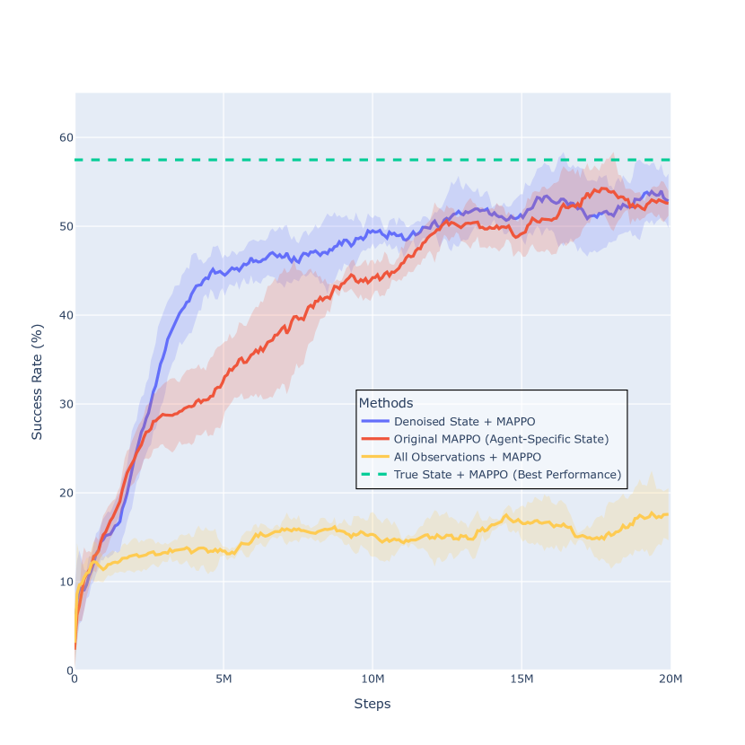
Figure 5. Policy learning performance of MAPPO with agent-specific states (in MAPPO’s vanilla implementation), joint histories, true states, and states predicted by diffusion models.

References

• (1)
• Ada et al. (2024) Suzan Ece Ada, Erhan Oztop, and Emre Ugur. 2024. Diffusion policies for out-of-distribution generalization in offline reinforcement learning. IEEE Robotics and Automation Letters (2024).
• Amato et al. (2013) Christopher Amato, Girish Chowdhary, Alborz Geramifard, N Kemal Üre, and Mykel J Kochenderfer. 2013. Decentralized control of partially observable Markov decision processes. In 52nd IEEE Conference on Decision and Control. IEEE, 2398–2405.
• Brehmer et al. (2024) Johann Brehmer, Joey Bose, Pim De Haan, and Taco S Cohen. 2024. EDGI: Equivariant diffusion for planning with embodied agents. Advances in Neural Information Processing Systems 36 (2024).
• Ceylan et al. (2023) Duygu Ceylan, Chun-Hao P Huang, and Niloy J Mitra. 2023. Pix2video: Video editing using image diffusion. In Proceedings of the IEEE/CVF International Conference on Computer Vision. 23206–23217.
• Chen et al. (2020) Ting Chen, Simon Kornblith, Mohammad Norouzi, and Geoffrey Hinton. 2020. A simple framework for contrastive learning of visual representations. In International conference on machine learning. PMLR, 1597–1607.
• Chen et al. (2023) Zoey Chen, Sho Kiami, Abhishek Gupta, and Vikash Kumar. 2023. Genaug: Retargeting behaviors to unseen situations via generative augmentation. arXiv preprint arXiv:2302.06671 (2023).
• Chi et al. (2023) Cheng Chi, Zhenjia Xu, Siyuan Feng, Eric Cousineau, Yilun Du, Benjamin Burchfiel, Russ Tedrake, and Shuran Song. 2023. Diffusion policy: Visuomotor policy learning via action diffusion. The International Journal of Robotics Research (2023), 02783649241273668.
• De Gennaro and Jadbabaie (2006) Maria Carmela De Gennaro and Ali Jadbabaie. 2006. Decentralized control of connectivity for multi-agent systems. In Proceedings of the 45th IEEE Conference on Decision and Control. IEEE, 3628–3633.
• Doersch (2016) Carl Doersch. 2016. Tutorial on variational autoencoders. arXiv preprint arXiv:1606.05908 (2016).
• Dong et al. (2022) Heng Dong, Tonghan Wang, Jiayuan Liu, and Chongjie Zhang. 2022. Low-rank modular reinforcement learning via muscle synergy. Advances in Neural Information Processing Systems 35 (2022), 19861–19873.
• Efron (2011) Bradley Efron. 2011. Tweedie’s formula and selection bias. J. Amer. Statist. Assoc. 106, 496 (2011), 1602–1614.
• Ellis et al. (2023) Benjamin Ellis, Jonathan Cook, Skander Moalla, Mikayel Samvelyan, Mingfei Sun, Anuj Mahajan, Jakob Nicolaus Foerster, and Shimon Whiteson. 2023. SMACv2: An Improved Benchmark for Cooperative Multi-Agent Reinforcement Learning. In Thirty-seventh Conference on Neural Information Processing Systems Datasets and Benchmarks Track. https://openreview.net/forum?id=5OjLGiJW3u
• Esser et al. (2024) Patrick Esser, Sumith Kulal, Andreas Blattmann, Rahim Entezari, Jonas Müller, Harry Saini, Yam Levi, Dominik Lorenz, Axel Sauer, Frederic Boesel, et al. 2024. Scaling rectified flow transformers for high-resolution image synthesis. In Forty-first International Conference on Machine Learning.
• Foerster et al. (2016) Jakob Foerster, Ioannis Alexandros Assael, Nando de Freitas, and Shimon Whiteson. 2016. Learning to communicate with deep multi-agent reinforcement learning. In Advances in Neural Information Processing Systems. 2137–2145.
• Goldman and Zilberstein (2003) Claudia V Goldman and Shlomo Zilberstein. 2003. Optimizing information exchange in cooperative multi-agent systems. In Proceedings of the second international joint conference on Autonomous agents and multiagent systems. 137–144.
• Guo et al. (2024) Yuwei Guo, Ceyuan Yang, Anyi Rao, Zhengyang Liang, Yaohui Wang, Yu Qiao, Maneesh Agrawala, Dahua Lin, and Bo Dai. 2024. AnimateDiff: Animate Your Personalized Text-to-Image Diffusion Models without Specific Tuning. In The Twelfth International Conference on Learning Representations.
• Han et al. (2019) Dongqi Han, Kenji Doya, and Jun Tani. 2019. Variational recurrent models for solving partially observable control tasks. arXiv preprint arXiv:1912.10703 (2019).
• Han and Gmytrasiewicz (2018) Yanlin Han and Piotr Gmytrasiewicz. 2018. Learning others’ intentional models in multi-agent settings using interactive POMDPs. Advances in Neural Information Processing Systems 31 (2018).
• Hansen-Estruch et al. (2023) Philippe Hansen-Estruch, Ilya Kostrikov, Michael Janner, Jakub Grudzien Kuba, and Sergey Levine. 2023. Idql: Implicit q-learning as an actor-critic method with diffusion policies. arXiv preprint arXiv:2304.10573 (2023).
• Hausknecht and Stone (2015) Matthew Hausknecht and Peter Stone. 2015. Deep recurrent q-learning for partially observable mdps. In 2015 aaai fall symposium series.
• Ho et al. (2022a) Jonathan Ho, William Chan, Chitwan Saharia, Jay Whang, Ruiqi Gao, Alexey Gritsenko, Diederik P Kingma, Ben Poole, Mohammad Norouzi, David J Fleet, et al. 2022a. Imagen video: High definition video generation with diffusion models. arXiv preprint arXiv:2210.02303 (2022).
• Ho et al. (2020) Jonathan Ho, Ajay Jain, and Pieter Abbeel. 2020. Denoising diffusion probabilistic models. Advances in neural information processing systems 33 (2020), 6840–6851.
• Ho et al. (2022b) Jonathan Ho, Tim Salimans, Alexey Gritsenko, William Chan, Mohammad Norouzi, and David J Fleet. 2022b. Video diffusion models. Advances in Neural Information Processing Systems 35 (2022), 8633–8646.
• Janner et al. (2022) Michael Janner, Yilun Du, Joshua B Tenenbaum, and Sergey Levine. 2022. Planning with diffusion for flexible behavior synthesis. arXiv preprint arXiv:2205.09991 (2022).
• Jiang et al. (2018) Jiechuan Jiang, Chen Dun, Tiejun Huang, and Zongqing Lu. 2018. Graph convolutional reinforcement learning. arXiv preprint arXiv:1810.09202 (2018).
• Jiang and Lu (2018) Jiechuan Jiang and Zongqing Lu. 2018. Learning attentional communication for multi-agent cooperation. In Advances in Neural Information Processing Systems. 7254–7264.
• Kadkhodaie et al. (2023) Zahra Kadkhodaie, Florentin Guth, Eero P Simoncelli, and Stéphane Mallat. 2023. Generalization in diffusion models arises from geometry-adaptive harmonic representation. arXiv preprint arXiv:2310.02557 (2023).
• Kadkhodaie and Simoncelli (2020) Zahra Kadkhodaie and Eero P Simoncelli. 2020. Solving linear inverse problems using the prior implicit in a denoiser. arXiv preprint arXiv:2007.13640 (2020).
• Kaelbling et al. (1998) Leslie Pack Kaelbling, Michael L Littman, and Anthony R Cassandra. 1998. Planning and acting in partially observable stochastic domains. Artificial intelligence 101, 1-2 (1998), 99–134.
• Kang et al. (2022) Yipeng Kang, Tonghan Wang, Qianlan Yang, Xiaoran Wu, and Chongjie Zhang. 2022. Non-linear coordination graphs. Advances in Neural Information Processing Systems 35 (2022), 25655–25666.
• Kao and Subramanian (2022) Hsu Kao and Vijay Subramanian. 2022. Common information based approximate state representations in multi-agent reinforcement learning. In International Conference on Artificial Intelligence and Statistics. PMLR, 6947–6967.
• Kim et al. (2020) Woojun Kim, Jongeui Park, and Youngchul Sung. 2020. Communication in multi-agent reinforcement learning: Intention sharing. In International conference on learning representations.
• Lesser et al. (2003) Victor Lesser, Charles L Ortiz, and Milind Tambe. 2003. Distributed sensor networks: A multiagent perspective. Vol. 9. Springer Science & Business Media.
• Liang et al. (2023) Zhixuan Liang, Yao Mu, Mingyu Ding, Fei Ni, Masayoshi Tomizuka, and Ping Luo. 2023. Adaptdiffuser: Diffusion models as adaptive self-evolving planners. arXiv preprint arXiv:2302.01877 (2023).
• Lipman et al. (2022) Yaron Lipman, Ricky TQ Chen, Heli Ben-Hamu, Maximilian Nickel, and Matthew Le. 2022. Flow Matching for Generative Modeling. In The Eleventh International Conference on Learning Representations.
• Liu et al. (2023) Xingchao Liu, Chengyue Gong, et al. 2023. Flow Straight and Fast: Learning to Generate and Transfer Data with Rectified Flow. In The Eleventh International Conference on Learning Representations.
• Loch and Singh (1998) John Loch and Satinder Singh. 1998. Using Eligibility Traces to Find the Best Memoryless Policy in Partially Observable Markov Decision Processes.. In ICML, Vol. 98. Citeseer, 323–331.
• Lou et al. (2024) Aaron Lou, Chenlin Meng, and Stefano Ermon. 2024. Discrete Diffusion Modeling by Estimating the Ratios of the Data Distribution. In Forty-first International Conference on Machine Learning.
• Lu et al. (2024) Cong Lu, Philip Ball, Yee Whye Teh, and Jack Parker-Holder. 2024. Synthetic experience replay. Advances in Neural Information Processing Systems 36 (2024).
• MacDermed and Isbell (2013) Liam C MacDermed and Charles L Isbell. 2013. Point based value iteration with optimal belief compression for Dec-POMDPs. Advances in neural information processing systems 26 (2013).
• Miyasawa et al. (1961) Koichi Miyasawa et al. 1961. An empirical Bayes estimator of the mean of a normal population. Bull. Inst. Internat. Statist 38, 181-188 (1961), 1–2.
• Modi et al. (2001) Pragnesh Jay Modi, Hyuckchul Jung, Milind Tambe, Wei-Min Shen, and Shriniwas Kulkarni. 2001. A dynamic distributed constraint satisfaction approach to resource allocation. In Principles and Practice of Constraint Programming—CP 2001: 7th International Conference, CP 2001 Paphos, Cyprus, November 26–December 1, 2001 Proceedings 7. Springer, 685–700.
• Mohan et al. (2019) Sreyas Mohan, Zahra Kadkhodaie, Eero P Simoncelli, and Carlos Fernandez-Granda. 2019. Robust and interpretable blind image denoising via bias-free convolutional neural networks. arXiv preprint arXiv:1906.05478 (2019).
• Mohan et al. (2020) Sreyas Mohan, Zahra Kadkhodaie, Eero P Simoncelli, and Carlos Fernandez-Granda. 2020. Robust And Interpretable Blind Image Denoising Via Bias-Free Convolutional Neural Networks. In International Conference on Learning Representations.
• Muglich et al. (2022) Darius Muglich, Luisa M Zintgraf, Christian A Schroeder De Witt, Shimon Whiteson, and Jakob Foerster. 2022. Generalized beliefs for cooperative AI. In International Conference on Machine Learning. PMLR, 16062–16082.
• Nair et al. (2005) Ranjit Nair, Pradeep Varakantham, Milind Tambe, and Makoto Yokoo. 2005. Networked distributed POMDPs: A synthesis of distributed constraint optimization and POMDPs. In AAAI, Vol. 5. 133–139.
• Oliehoek et al. (2016) Frans A Oliehoek, Christopher Amato, et al. 2016. A concise introduction to decentralized POMDPs. Vol. 1. Springer.
• Omidshafiei et al. (2017) Shayegan Omidshafiei, Jason Pazis, Christopher Amato, Jonathan P How, and John Vian. 2017. Deep decentralized multi-task multi-agent reinforcement learning under partial observability. In International Conference on Machine Learning. PMLR, 2681–2690.
• Peng et al. (2017) Peng Peng, Ying Wen, Yaodong Yang, Quan Yuan, Zhenkun Tang, Haitao Long, and Jun Wang. 2017. Multiagent bidirectionally-coordinated nets: Emergence of human-level coordination in learning to play starcraft combat games. arXiv preprint arXiv:1703.10069 (2017).
• Pynadath and Tambe (2002) David V Pynadath and Milind Tambe. 2002. The communicative multiagent team decision problem: Analyzing teamwork theories and models. Journal of artificial intelligence research 16 (2002), 389–423.
• Qu et al. (2020) Chao Qu, Hui Li, Chang Liu, Junwu Xiong, Wei Chu, Weiqiang Wang, Yuan Qi, Le Song, et al. 2020. Intention propagation for multi-agent reinforcement learning. (2020).
• Raileanu et al. (2018) Roberta Raileanu, Emily Denton, Arthur Szlam, and Rob Fergus. 2018. Modeling others using oneself in multi-agent reinforcement learning. In International conference on machine learning. PMLR, 4257–4266.
• Raphan and Simoncelli (2011) Martin Raphan and Eero P Simoncelli. 2011. Least squares estimation without priors or supervision. Neural computation 23, 2 (2011), 374–420.
• Rashid et al. (2018) Tabish Rashid, Mikayel Samvelyan, Christian Schroeder Witt, Gregory Farquhar, Jakob Foerster, and Shimon Whiteson. 2018. QMIX: Monotonic Value Function Factorisation for Deep Multi-Agent Reinforcement Learning. In International Conference on Machine Learning. 4292–4301.
• Robbins (1992) Herbert E Robbins. 1992. An empirical Bayes approach to statistics. In Breakthroughs in Statistics: Foundations and basic theory. Springer, 388–394.
• Rombach et al. (2022) Robin Rombach, Andreas Blattmann, Dominik Lorenz, Patrick Esser, and Björn Ommer. 2022. High-resolution image synthesis with latent diffusion models. In Proceedings of the IEEE/CVF conference on computer vision and pattern recognition. 10684–10695.
• Ronneberger et al. (2015) Olaf Ronneberger, Philipp Fischer, and Thomas Brox. 2015. U-net: Convolutional networks for biomedical image segmentation. In Medical image computing and computer-assisted intervention–MICCAI 2015: 18th international conference, Munich, Germany, October 5-9, 2015, proceedings, part III 18. Springer, 234–241.
• Saldi et al. (2019) Naci Saldi, Tamer Başar, and Maxim Raginsky. 2019. Approximate Nash equilibria in partially observed stochastic games with mean-field interactions. Mathematics of Operations Research 44, 3 (2019), 1006–1033.
• Samvelyan et al. (2019) Mikayel Samvelyan, Tabish Rashid, Christian Schroeder de Witt, Gregory Farquhar, Nantas Nardelli, Tim G. J. Rudner, Chia-Man Hung, Philiph H. S. Torr, Jakob Foerster, and Shimon Whiteson. 2019. The StarCraft Multi-Agent Challenge. CoRR abs/1902.04043 (2019).
• Spaan and Vlassis (2005) Matthijs TJ Spaan and Nikos Vlassis. 2005. Perseus: Randomized point-based value iteration for POMDPs. Journal of artificial intelligence research 24 (2005), 195–220.
• Srinivasan et al. (2018) Sriram Srinivasan, Marc Lanctot, Vinicius Zambaldi, Julien Pérolat, Karl Tuyls, Rémi Munos, and Michael Bowling. 2018. Actor-critic policy optimization in partially observable multiagent environments. Advances in neural information processing systems 31 (2018).
• Sukhbaatar et al. (2016) Sainbayar Sukhbaatar, Rob Fergus, et al. 2016. Learning multiagent communication with backpropagation. Advances in neural information processing systems 29 (2016).
• Sunehag et al. (2018) Peter Sunehag, Guy Lever, Audrunas Gruslys, Wojciech Marian Czarnecki, Vinicius Zambaldi, Max Jaderberg, Marc Lanctot, Nicolas Sonnerat, Joel Z Leibo, Karl Tuyls, et al. 2018. Value-decomposition networks for cooperative multi-agent learning based on team reward. In Proceedings of the 17th International Conference on Autonomous Agents and MultiAgent Systems. International Foundation for Autonomous Agents and Multiagent Systems, 2085–2087.
• Varakantham et al. (2006) Pradeep Varakantham, Ranjit Nair, Milind Tambe, and Makoto Yokoo. 2006. Winning back the cup for distributed POMDPs: planning over continuous belief spaces. In Proceedings of the fifth international joint conference on Autonomous agents and multiagent systems. 289–296.
• Wang et al. (2020b) Rose E Wang, Michael Everett, and Jonathan P How. 2020b. R-MADDPG for partially observable environments and limited communication. arXiv preprint arXiv:2002.06684 (2020).
• Wang et al. (2020a) Tonghan Wang, Heng Dong, Victor Lesser, and Chongjie Zhang. 2020a. ROMA: Multi-Agent Reinforcement Learning with Emergent Roles. In Proceedings of the 37th International Conference on Machine Learning.
• Wang et al. (2020c) Tonghan Wang, Tarun Gupta, Anuj Mahajan, Bei Peng, Shimon Whiteson, and Chongjie Zhang. 2020c. RODE: Learning Roles to Decompose Multi-Agent Tasks. In International Conference on Learning Representations.
• Wang et al. (2019) Tonghan Wang, Jianhao Wang, Chongyi Zheng, and Chongjie Zhang. 2019. Learning Nearly Decomposable Value Functions Via Communication Minimization. In International Conference on Learning Representations.
• Wang et al. (2020d) Yihan Wang, Beining Han, Tonghan Wang, Heng Dong, and Chongjie Zhang. 2020d. DOP: Off-policy multi-agent decomposed policy gradients. In International conference on learning representations.
• Wen et al. (2022) Muning Wen, Jakub Kuba, Runji Lin, Weinan Zhang, Ying Wen, Jun Wang, and Yaodong Yang. 2022. Multi-agent reinforcement learning is a sequence modeling problem. Advances in Neural Information Processing Systems 35 (2022), 16509–16521.
• Wu et al. (2024) Xiaoran Wu, Zien Huang, and Chonghan Yu. 2024. Animating the Past: Reconstruct Trilobite via Video Generation. (2024). https://doi.org/10.12074/202410.00084
• Xu et al. (2020) Jing Xu, Fangwei Zhong, and Yizhou Wang. 2020. Learning multi-agent coordination for enhancing target coverage in directional sensor networks. Advances in Neural Information Processing Systems 33 (2020), 10053–10064.
• Xu et al. (2021) Zhiwei Xu, Yunpeng Bai, Dapeng Li, Bin Zhang, and Guoliang Fan. 2021. Side: State inference for partially observable cooperative multi-agent reinforcement learning. arXiv preprint arXiv:2105.06228 (2021).
• Xu et al. (2024) Zhiwei Xu, Hangyu Mao, Nianmin Zhang, Xin Xin, Pengjie Ren, Dapeng Li, Bin Zhang, Guoliang Fan, Zhumin Chen, Changwei Wang, et al. 2024. Beyond Local Views: Global State Inference with Diffusion Models for Cooperative Multi-Agent Reinforcement Learning. arXiv preprint arXiv:2408.09501 (2024).
• Yang et al. (2008) Peng Yang, Randy A Freeman, and Kevin M Lynch. 2008. Multi-agent coordination by decentralized estimation and control. IEEE Trans. Automat. Control 53, 11 (2008), 2480–2496.
• Yu et al. (2022) Chao Yu, Akash Velu, Eugene Vinitsky, Jiaxuan Gao, Yu Wang, Alexandre Bayen, and Yi Wu. 2022. The surprising effectiveness of ppo in cooperative multi-agent games. Advances in Neural Information Processing Systems 35 (2022), 24611–24624.
• Zhang and Lesser (2011) Chongjie Zhang and Victor Lesser. 2011. Coordinated multi-agent reinforcement learning in networked distributed POMDPs. In Proceedings of the AAAI Conference on Artificial Intelligence, Vol. 25. 764–770.
• Zhang et al. (2020) Haifeng Zhang, Weizhe Chen, Zeren Huang, Minne Li, Yaodong Yang, Weinan Zhang, and Jun Wang. 2020. Bi-level actor-critic for multi-agent coordination. In Proceedings of the AAAI Conference on Artificial Intelligence, Vol. 34. 7325–7332.
• Zhang et al. (2021b) Kaiqing Zhang, Zhuoran Yang, and Tamer Başar. 2021b. Multi-agent reinforcement learning: A selective overview of theories and algorithms. Handbook of reinforcement learning and control (2021), 321–384.
• Zhang et al. (2021a) Weinan Zhang, Xihuai Wang, Jian Shen, and Ming Zhou. 2021a. Model-based multi-agent policy optimization with adaptive opponent-wise rollouts. arXiv preprint arXiv:2105.03363 (2021).