Nonlinear Stochastic Gradient Descent and Heavy-tailed Noise: A Unified Framework and High-probability Guarantees

Abstract

We study high-probability convergence in online learning, in the presence of heavy-tailed noise. To combat the heavy tails, a general framework of nonlinear SGD methods is considered, subsuming several popular nonlinearities like sign, quantization, component-wise and joint clipping. In our work the nonlinearity is treated in a black-box manner, allowing us to establish unified guarantees for a broad range of nonlinear methods. For symmetric noise and non-convex costs we establish convergence of gradient norm-squared, at a rate $\widetilde{\mathcal{O}}(t^{-\nicefrac{{1}}{{4}}})$, while for the last iterate of strongly convex costs we establish convergence to the population optima, at a rate $\mathcal{O}(t^{-\zeta})$, where $\zeta\in(0,1)$ depends on noise and problem parameters. Further, if the noise is a (biased) mixture of symmetric and non-symmetric components, we show convergence to a neighbourhood of stationarity, whose size depends on the mixture coefficient, nonlinearity and noise. Compared to state-of-the-art, who only consider clipping and require unbiased noise with bounded $p$-th moments, $p\in(1,2]$, we provide guarantees for a broad class of nonlinearities, without any assumptions on noise moments. While the rate exponents in state-of-the-art depend on noise moments and vanish as $p\rightarrow 1$, our exponents are constant and strictly better whenever $p<6/5$ for non-convex and $p<8/7$ for strongly convex costs. Experiments validate our theory, demonstrating noise symmetry in real-life settings and showing that clipping is not always the optimal nonlinearity, further underlining the value of a general framework.

1 Introduction

Stochastic optimization is a well-studied problem, e.g., Robbins and Monro, (1951); Nemirovski et al., (2009), where the goal is to minimize an expected cost, without knowing the underlying probability distribution. Formally, the problem is cast as

$$\operatorname*{arg\,min}_{{\mathbf{x}}\in\mathbb{R}^{d}}\left\{f({\mathbf{x}})\triangleq\mathbb{E}_{\upsilon\sim\Upsilon}[\ell({\mathbf{x}};\upsilon)]\right\},$$ (1)

where ${\mathbf{x}}\in\mathbb{R}^{d}$ represents model parameters, $\ell:\mathbb{R}^{d}\times\mathcal{V}\mapsto\mathbb{R}$ is a loss function, $\upsilon\in\mathcal{V}$ is a random sample distributed according to the unknown distribution $\Upsilon$, while $f:\mathbb{R}^{d}\mapsto\mathbb{R}$ is commonly known as the population cost. Many modern machine learning applications, such as classification and regression, are modeled using (1).

Perhaps the most popular method to solve (1) is stochastic gradient descent (SGD) Robbins and Monro, (1951), whose popularity stems from low computation cost and incredible empirical success Bottou, (2010); Hardt et al., (2016). Convergence guarantees of SGD have been studied extensively Moulines and Bach, (2011); Rakhlin et al., (2012); Bottou et al., (2018). Classical convergence results are mostly concerned with mean-squared error (MSE) convergence, characterizing the average performance across many runs of the algorithm. However, due to significant computational cost of a single run of an algorithm in many modern machine learning applications, it is often infeasible to perform multiple runs Harvey et al., (2019); Davis et al., (2021). As such, many applications require more fine-grained results, such as high-probability convergence, which characterize the behaviour of an algorithm with respect to a single run.

Another striking feature of existing works is the assumption that the gradient noise has light-tails or uniformly bounded variance Rakhlin et al., (2012); Ghadimi and Lan, (2012, 2013), which represents a major limitation in many modern applications, see Simsekli et al., 2019a ; Simsekli et al., 2019b . For example, Zhang et al., (2020) show that the gradient noise distribution during training of large attention models resembles a Levy $\alpha$-stable distribution, with $\alpha<2$, which has unbounded variance. To better model this phenomena, the authors propose the bounded $p$-th moment assumption, i.e.,

$$\mathbb{E}_{\upsilon\sim\Upsilon}\|\nabla\ell({\mathbf{x}},\upsilon)-\nabla f({\mathbf{x}})\|^{p}\leq\sigma^{p},$$ (BM)

for every ${\mathbf{x}}\in\mathbb{R}^{d}$ and some $p\in(1,2]$, $\sigma>0$, subsuming the bounded variance case for $p=2$. Under this assumption, Zhang et al., (2020) show that SGD fails to converge for any fixed step-size. The clipped variant of SGD solves this problem and achieves optimal MSE convergence rate for smooth non-convex losses. Along with addressing heavy-tailed noise, clipped SGD also addresses non-smoothness of the cost Zhang et al., (2019), ensures differential privacy Zhang et al., (2022) and robustness to malicious nodes in distributed learning Yu and Kar, (2023). While popular, clipping is not the only nonlinearity employed in practice. Sign and quantized variants of SGD improve communication efficiency in distributed learning Alistarh et al., (2017); Bernstein et al., 2018a ; Gandikota et al., (2021). Sign SGD achieves performance on par with state-of-the-art adaptive methods Crawshaw et al., (2022), and is robust to faulty and malicious users Bernstein et al., 2018b . Normalized SGD is empirically observed to accelerate neural network training Hazan et al., (2015); You et al., (2019); Cutkosky and Mehta, (2020) and facilitates privacy Das et al., (2021); Yang et al., (2022), while Zhang et al., (2020) empirically observe that component-wise clipping converges faster than the joint one, showing better dependence on problem dimension. Although assumption (BM) helps bridge the gap between theory and practice, the downside is that the resulting convergence rates have exponents which explicitly depend on the noise moment and vanish as $p\rightarrow 1$. This seems to contradict the strong performance of nonlinear SGD methods observed in practice and fails to explain the empirical success of nonlinear SGD, e.g., during training of models such as neural networks, in the presence of heavy-tailed noise. A growing body of works recently provided strong evidence that the stochastic noise during training of neural networks is symmetric, by studying the empirical distribution of gradient noise during training. For example, Bernstein et al., 2018a ; Bernstein et al., 2018b show that histograms of gradient noise during training of different Resnet architectures on CIFAR-10 and Imagenet data exhibit strong symmetry under various batch sizes, see their Figures 2 (in both works). Similarly, Chen et al., (2020) demonstrate strong symmetry of gradient distributions during training of convolutional neural networks (CNN) on CIFAR-10 and MNIST data, see their Figures 1-3. Barsbey et al., (2021) show that the histograms of weights of a CNN layer trained on MNIST data almost identically match samples simulated from a symmetric $\alpha$-stable distribution, see their Figure 2. Finally, Battash et al., (2024) show that a heavy-tailed symmetric $\alpha$-stable distribution is a much better fit for the stochastic gradient noise than a Gaussian, for a myriad of deep learning architectures and datasets, see their Tables 1-3. We provide further empirical evidence of this phenomena, see Section 4 and the Appendix. Relying on a generalization of the central limit theorem (CLT), Simsekli et al., 2019b ; Peluchetti et al., (2020); Gurbuzbalaban et al., (2021); Barsbey et al., (2021) theoretically show that symmetric heavy-tailed noises are appropriate models in many practical settings, e.g., when training neural networks with mini-batch SGD using a large batch size. In contrast, works using assumption (BM) are inherently oblivious to this widely observed phenomena. The goal of this paper is to study high-probability guarantees of nonlinear SGD methods in the presence of symmetric heavy-tailed noise and the benefits symmetry brings.

Table 1: High-probability guarantees of SGD methods under heavy-tailed noise. Online indicates whether a method uses a time-varying step-size and is applicable in the online setting (indicated by lower-case $t$), or if it uses a fixed step-size and requires a preset time horizon which is optimized to achieve the best rate and works only in the offline setting (indicated by upper-case $T$). The value $\beta\in(0,1)$ represents the failure probability, while $\widetilde{\mathcal{O}}(\cdot)$ hides factors poly-logarithmic in time $t$. All the works achieve a poly-logarithmic dependence on the failure probability $\beta$ (i.e., contain a multiplicative factor of $\log(\nicefrac{{1}}{{\beta}})$ in the bound), which is hidden under the big O notation, for ease of presentation.

Cost	Work	Nonlinearity	Noise	Online	Rate
Non-convex	Nguyen et al., 2023a	Clipping only	$\begin{subarray}{c}\text{\scriptsize{unbiased, bounded}}\\ \text{\scriptsize{moment of order }}\\ p\in(1,2]\end{subarray}$	✔	$\widetilde{\mathcal{O}}\left(t^{\frac{2(1-p)}{(3p-2)}}\right)$
	Sadiev et al., (2023)			✗	$\mathcal{O}\left(T^{\frac{(1-p)}{p}}\right)$
	This paper	$\begin{subarray}{c}\text{\scriptsize Component-wise}\\ \text{\scriptsize and joint}\end{subarray}$	$\begin{subarray}{c}\text{\scriptsize{symmetric pdf,}}\\ \text{\scriptsize{positive around}}\\ \text{\scriptsize zero}\end{subarray}$	✔	$\widetilde{\mathcal{O}}\left(t^{-\nicefrac{{1}}{{4}}}\right)^{\dagger}$
$\begin{subarray}{c}\text{\scriptsize Strongly}\\ \text{\scriptsize convex}\end{subarray}$	Sadiev et al., (2023)	Clipping only	$\begin{subarray}{c}\text{\scriptsize{unbiased, bounded}}\\ \text{\scriptsize{moment of order }}\\ p\in(1,2]\end{subarray}$	✗	$\mathcal{O}\left(T^{\frac{2(1-p)}{p}}\right)$
	$\begin{subarray}{c}\text{\scriptsize This paper - weighted}\\ \text{\scriptsize average of iterates}\end{subarray}$	$\begin{subarray}{c}\text{\scriptsize Component-wise}\\ \text{\scriptsize and joint}\end{subarray}$	$\begin{subarray}{c}\text{\scriptsize{symmetric pdf,}}\\ \text{\scriptsize{positive around}}\\ \text{\scriptsize zero}\end{subarray}$	✔	$\widetilde{\mathcal{O}}\left(t^{-\nicefrac{{1}}{{4}}}\right)^{\dagger}$
	This paper - last iterate			✔	$\mathcal{O}\left(t^{-\zeta}\right)^{\S}$

• We derive convergence guarantees for a wide range of step-sizes of the form $\alpha_{t}=\nicefrac{{a}}{{(t+1)^{\delta}}}$, where $a>0$, $\delta\in(\nicefrac{{2}}{{3}},1)$, with the resulting convergence rate depending on $\delta$. The best rate, shown in the table, is achieved for the choice $\delta=\nicefrac{{3}}{{4}}$.

• The rate $\zeta\in(0,1)$ depends on the choice of nonlinearity, noise and problem related parameters, see Section 3 and Appendix D. We provide examples of noise for which $\zeta>\nicefrac{{2(p-1)}}{{p}}$, see Examples 1-4 ahead.

Literature Review.

We now review the literature on high-probability convergence of SGD and its variants. Initial works on high-probability convergence of stochastic gradient methods considered light-tailed noise and include Nemirovski et al., (2009); Lan, (2012); Hazan and Kale, (2014); Harvey et al., (2019); Ghadimi and Lan, (2013); Li and Orabona, (2020). Subsequent works Gorbunov et al., (2020, 2021); Parletta et al., (2022) generalized these results to noise with bounded variance. Tsai et al., (2022) study clipped SGD, assuming the variance is bounded by iterate distance, while Li and Liu, (2022); Eldowa and Paudice, (2023); Madden et al., (2024) consider sub-Weibull noise. Recent works Liu et al., 2023a ; Eldowa and Paudice, (2023) remove restrictive assumptions, like bounded stochastic gradients and domain. Sadiev et al., (2023) show that even with bounded variance and smooth, strongly-convex functions, vanilla SGD cannot achieve an exponential tail decay, implying that the complexity of achieving a high-probability bound for SGD can be much worse than that of the corresponding MSE bound. As such, nonlinear SGD is used to handle tails heavier than sub-Gaussian. Recent works consider a class of heavy-tailed noises satisfying (BM), e.g., Nguyen et al., 2023a ; Nguyen et al., 2023b ; Sadiev et al., (2023); Liu et al., 2023b . Nguyen et al., 2023a ; Nguyen et al., 2023b study high-probability convergence of clipped SGD for convex and non-convex minimization, Sadiev et al., (2023) study clipped SGD for optimization and variational inequality problems, while Liu et al., 2023b study accelerated variants of clipped SGD for smooth losses. It is worth mentioning Puchkin et al., (2023), who show that clipped SGD achieves the optimal $\mathcal{O}\left(T^{-1}\right)$ rate for smooth, strongly convex costs, under a class of heavy-tailed noises with possibly unbounded first moments. However, their noise assumption is difficult to verify, as it requires computing convolutions of order $k$, for all $k\in\mathbb{N}$. Additionally, they use a median-of-means gradient estimator, which requires evaluating multiple stochastic gradients per iteration and is not applicable in the online setting considered in this paper.

The works closest to ours are Nguyen et al., 2023a for online non-convex and Sadiev et al., (2023) for offline strongly convex problems. We present a detailed comparison in Table 1. Both works study only the clipping operator and use assumption (BM). For non-convex costs, Nguyen et al., 2023a achieve the optimal rate $\widetilde{\mathcal{O}}\left(t^{\nicefrac{{2(1-p)}}{{(3p-2)}}}\right)$, while Sadiev et al., (2023) achieve the optimal rate $\mathcal{O}\left(T^{\nicefrac{{2(1-p)}}{{p}}}\right)$ for strongly convex costs. Compared to them, we consider a much broader class of nonlinearities in the presence of noise with symmetric density with no moment requirements, achieving the near-optimal rate $\widetilde{\mathcal{O}}\left(t^{-\nicefrac{{1}}{{4}}}\right)$ for non-convex costs and extending it to the weighted average of iterates for strongly convex costs. Crucially, our rate exponent is independent of noise and problem parameters, which is not the case with Nguyen et al., 2023a ; Sadiev et al., (2023). Our rates are strictly better whenever $p<6/5$ for non-convex and $p<8/7$ for strongly convex costs. Additionally, we establish convergence of the last iterate for strongly convex costs, with rate $\mathcal{O}\left(t^{-\zeta}\right)$, where $\zeta\in(0,1)$ depends on noise, nonlinearity and other problem parameters. We give examples of noise regimes where our rate is better than the one in Sadiev et al., (2023) (see Examples 1-4) and demonstrate numerically that clipping is not always the best nonlinearity (see Section 4), further highlighting the importance and usefulness of our general framework. Finally, it is worth mentioning Jakovetić et al., (2023), who provide MSE, asymptotic normality and almost sure guarantees of the same nonlinear framework for strongly convex costs and noises with symmetric PDF, positive around zero and bounded first moments. Our work differs in that we study high-probability convergence, relax the moment conditions and allow for non-convex costs. The latter is achieved by providing a novel characterization of the interplay of the “denoised” nonlinear gradient and the true gradient (see Lemma 3.2).

Contributions.

Our contributions are as follows.
1. We study convergence in high probability of a unified framework of nonlinear SGD, in the presence of heavy-tailed noise and widely observed noise symmetry, making no assumptions on noise moments. The nonlinear map is treated in a black-box manner, subsuming many popular nonlinearities, like sign, normalization, clipping and quantization. To the best of our knowledge, we provide the first high-probability results under heavy-tailed noise for methods such as sign, quantized and component-wise clipped SGD.
2. For non-convex costs, we show convergence of gradient norm-squared, at a near-optimal rate $\widetilde{\mathcal{O}}\left(t^{-\nicefrac{{1}}{{4}}}\right)$. The exponent in our rate is constant, independent of noise and problem parameters, which is not the case with state-of-the-art Nguyen et al., 2023a . Our rate is strictly better than state-of-the-art whenever the noise has bounded moments of order $p<\frac{6}{5}$.
3. For strongly convex costs we show convergence of the weighted average of iterates, at the same rate $\widetilde{\mathcal{O}}\left(t^{-\nicefrac{{1}}{{4}}}\right)$. Our rate dominates the state-of-the-art Sadiev et al., (2023) whenever the noise has bounded moments of order $p<\frac{8}{7}$, while being applicable in the online setting, which is not the case for Sadiev et al., (2023). For the last iterate we show convergence at a rate $\mathcal{O}\left(t^{-\zeta}\right)$, where $\zeta\in(0,1)$ depends on noise, nonlinearity and problem parameters, but remains bounded away from zero even for unbounded noise moments.
4. We extend our results beyond symmetric noise, by considering a mixture of symmetric and non-symmetric components. For non-convex costs we show convergence to a neighbourhood of stationarity, at a rate $\widetilde{\mathcal{O}}(t^{-\nicefrac{{1}}{{4}}})$, where the size of the neighbourhood depends on the mixture coefficient, nonlinearity and noise. While Nguyen et al., 2023a achieve convergence under condition (BM), which does not require symmetry, they explicitly require unbiased noise, which is not the case for our mixture noise, allowing it to be biased.
5. Compared to state-of-the-art Nguyen et al., 2023a ; Sadiev et al., (2023), who only consider clipping, require bounded noise moments of order $p\in(1,2]$ and whose rates vanish as $p\rightarrow 1$, we consider a much broader class of nonlinearities, relax the moment condition and provide convergence rates with constant exponents. We provide further empirical evidence that the stochastic noise during training of deep learning models on real data tends to be strongly symmetric, as well as a toy example which shows that clipping is not always the optimal choice of nonlinearity, further reinforcing the importance of our general framework.

Paper Organization.

The rest of the paper is organized as follows. Section 2 outlines the proposed framework. Section 3 presents the main results. Section 4 provides numerical results. Section 5 concludes the paper. Appendix contains additional experiments and proofs omitted from the main body. The remainder of this section introduces the notation.

Notation.

The set of positive integers is denoted by $\mathbb{N}$. For $a\in\mathbb{N}$, the set of integers up to and including $a$ is denoted by $[a]=\{1,\ldots,a\}$. The sets of real numbers and $d$-dimensional vectors are denoted by $\mathbb{R}$ and $\mathbb{R}^{d}$. Regular and bold symbols denote scalars and vectors, i.e., $x\in\mathbb{R}$ and ${\mathbf{x}}\in\mathbb{R}^{d}$. The Euclidean inner product and induced norm are denoted by $\langle\cdot,\cdot\rangle$ and $\|\cdot\|$.

2 Proposed Framework

To solve (1) in the online setting, under the presence of heavy-tailed noise, we use the nonlinear SGD framework. The algorithm starts by choosing a deterministic initial model ${\mathbf{x}}^{(1)}\in\mathbb{R}^{d}$, a step-size schedule $\{\alpha_{t}\}_{t\in\mathbb{N}}$ and a nonlinear map $\boldsymbol{\Psi}:\mathbb{R}^{d}\mapsto\mathbb{R}^{d}$. In iteration $t=1,2,\ldots$, the method performs as follows: a first-order oracle is queried, which returns the gradient of the loss $\ell$ evaluated at the current model ${\mathbf{x}^{(t)}}$ and a random sample $\upsilon^{(t)}$. Then, the model is updated as

$${\mathbf{x}^{(t+1)}}={\mathbf{x}^{(t)}}-\alpha_{t}\mathbf{\Psi}\left(\nabla\ell({\mathbf{x}^{(t)}};\upsilon^{(t)})\right),$$ (2)

where $\alpha_{t}>0$ is the step-size at iteration $t$. The method is summed up in Algorithm 1. We make the following assumption on the nonlinear map ${\boldsymbol{\Psi}}$.

Algorithm 1 Online Nonlinear SGD

1:Choice of nonlinearity ${\boldsymbol{\Psi}}:\mathbb{R}^{d}\mapsto\mathbb{R}^{d}$, model initialization ${\mathbf{x}}^{(1)}\in\mathbb{R}^{d}$, step-size schedule $\{\alpha_{t}\}_{t\in\mathbb{N}}$;

2:for t = 1,2,… do:

3:   Query the oracle and receive $\nabla\ell({\mathbf{x}^{(t)}};\upsilon^{(t)})$;

4:   Update ${\mathbf{x}^{(t+1)}}\leftarrow{\mathbf{x}^{(t)}}-\alpha_{t}\mathbf{\Psi}\left(\nabla\ell({\mathbf{x}^{(t)}};\upsilon^{(t)})\right)$;

Assumption 1.

The nonlinear map ${\boldsymbol{\Psi}}:\mathbb{R}^{d}\mapsto\mathbb{R}^{d}$ is either of the form ${\boldsymbol{\Psi}}({\mathbf{x}})={\boldsymbol{\Psi}}(x_{1},\dots,x_{d})=\left[\mathcal{N}_{1}(x_{1}),\dots,\mathcal{N}_{1}(x_{d})\right]^{\top}$ or ${\boldsymbol{\Psi}}({\mathbf{x}})={\mathbf{x}}\mathcal{N}_{2}(\|{\mathbf{x}}\|)$, where $\mathcal{N}_{1},\>\mathcal{N}_{2}:\mathbb{R}\mapsto\mathbb{R}$ satisfy:
1. $\mathcal{N}_{1},\mathcal{N}_{2}$ are continuous almost everywhere, $\mathcal{N}_{1}$ is piece-wise differentiable and the map $a\mapsto a\mathcal{N}_{2}(a)$ is non-decreasing.
2. $\mathcal{N}_{1}$ is monotonically non-decreasing and odd, while $\mathcal{N}_{2}$ is non-increasing.
3. $\mathcal{N}_{1}$ is either discontinuous at zero, or strictly increasing on $(-c_{1},c_{1})$, for some $c_{1}>0$, with $\mathcal{N}_{2}(a)>0$, for any $a>0$.
4. $\mathcal{N}_{1}$ and ${\mathbf{x}}\mathcal{N}_{2}(\|{\mathbf{x}}\|)$ are uniformly bounded, i.e., $|\mathcal{N}_{1}(x)|\leq C_{1}$ and $\|{\mathbf{x}}\mathcal{N}_{2}(\|{\mathbf{x}}\|)\|\leq C_{2}$, for some $C_{1},\>C_{2}>0$, and all $x\in\mathbb{R}$, ${\mathbf{x}}\in\mathbb{R}^{d}$.

Note that the fourth property implies $\|{\boldsymbol{\Psi}}({\mathbf{x}})\|\leq C$, where $C=C_{1}\sqrt{d}$ or $C=C_{2}$, depending on the form of nonlinearity. We will use the general bound $\|{\boldsymbol{\Psi}}({\mathbf{x}})\|\leq C$ for ease of presentation, and specialize where appropriate. Assumption 1 is satisfied by a wide class of nonlinearities, including:
1. Sign: $[{\boldsymbol{\Psi}}({\mathbf{x}})]_{i}=\text{sign}(x_{i}),\>i\in[d]$.
2. Component-wise clipping: $[{\boldsymbol{\Psi}}({\mathbf{x}})]_{i}=x_{i}$, for $|x_{i}|\leq m$, and $[{\boldsymbol{\Psi}}({\mathbf{x}})]_{i}=m\cdot\text{sign}(x_{i})$, for $|x_{i}|>m$, $i\in[d]$, for user-specified $m>0$.
3. Component-wise quantization: for each $i\in[d]$, let $[{\boldsymbol{\Psi}}({\mathbf{x}})]_{i}=r_{j}$, for $x_{i}\in(q_{j},q_{j+1}]$, with $j=0,\ldots,J-1$ and $-\infty=q_{0}<q_{1}<\ldots<q_{J}=+\infty$, where $r_{j}$,$q_{j}$ are chosen such that each component of ${\boldsymbol{\Psi}}$ is odd, and we have $\max_{j\in\{0,\ldots,J-1\}}|r_{j}|<R$, for user-specified $R>0$.
4. Normalization: ${\boldsymbol{\Psi}}({\mathbf{x}})=\frac{{\mathbf{x}}}{\left\|{\mathbf{x}}\right\|}$ and ${\boldsymbol{\Psi}}({\mathbf{x}})=\mathbf{0}$, if ${\mathbf{x}}=\mathbf{0}$.
5. Clipping: ${\boldsymbol{\Psi}}({\mathbf{x}})=\min\{1,\nicefrac{{M}}{{\|{\mathbf{x}}\|}}\}{\mathbf{x}}$, for user-specified $M>0$.

3 Theoretical Guarantees

In this section we present the main results of the paper. Subsection 3.1 presents the preliminaries, Subsection 3.2 presents the results for symmetric noises, while Subsection 3.3 presents the results for non-symmetric noises. The proofs can be found in the Appendix.

3.1 Preliminaries

In this section we provide the preliminaries and assumptions used in the analysis. To begin, we state the assumptions on the behaviour of the cost $f$.

Assumption 2.

The cost $f$ is bounded from below, has at least one stationary point and Lipschitz continuous gradients, i.e., $\inf_{{\mathbf{x}}\in\mathbb{R}^{d}}f({\mathbf{x}})>-\infty$, there exists a ${\mathbf{x}}^{\star}\in\mathbb{R}^{d}$, such that $\nabla f({\mathbf{x}}^{\star})=0$, and $\|\nabla f({\mathbf{x}})-\nabla f({\mathbf{y}})\|\leq L\|{\mathbf{x}}-{\mathbf{y}}\|$, for some $L>0$ and every ${\mathbf{x}},{\mathbf{y}}\in\mathbb{R}^{d}$.

Remark 1.

Boundedness from below and Lipschitz continuous gradients are standard for non-convex losses, e.g., Ghadimi and Lan, (2013). Since the goal in non-convex optimization is to reach a stationary point, it is natural to assume at least one such point exists, see Liu et al., 2023a ; Madden et al., (2024).

Remark 2.

It can be shown that Lipschitz continuous gradients imply the $L$-smothness inequality, i.e., $f({\mathbf{y}})\leq f({\mathbf{x}})+\langle\nabla f({\mathbf{x}}),{\mathbf{y}}-{\mathbf{x}}\rangle+\frac{L}{2}\|{\mathbf{x}}-{\mathbf{y}}\|^{2}$, for any ${\mathbf{x}},{\mathbf{y}}\in\mathbb{R}^{d}$, see Nesterov, (2018); Wright and Recht, (2022).

In addition to Assumption 2, we will sometimes use the following assumption.

Assumption 3.

The cost $f$ is strongly convex, i.e., $f({\mathbf{y}})\geq f({\mathbf{x}})+\langle\nabla f({\mathbf{x}}),{\mathbf{y}}-{\mathbf{x}}\rangle+\frac{\mu}{2}\|{\mathbf{x}}-{\mathbf{y}}\|^{2}$, for some $\mu>0$ and every ${\mathbf{x}},{\mathbf{y}}\in\mathbb{R}^{d}$.

Denote the infimum of $f$ by $f^{\star}\triangleq\inf_{{\mathbf{x}}\in\mathbb{R}^{d}}f({\mathbf{x}})$. Denote the set of stationary points of $f$ by $\mathcal{X}\triangleq\left\{{\mathbf{x}}^{\star}\in\mathbb{R}^{d}:\>\nabla f({\mathbf{x}}^{\star})=0\right\}$. By Assumption 2, it follows that $\mathcal{X}\neq\emptyset$. If in addition Assumption 3 holds, we have $\mathcal{X}=\{{\mathbf{x}}^{\star}\}$ and $f^{\star}=f({\mathbf{x}}^{\star})$, for some ${\mathbf{x}}^{\star}\in\mathbb{R}^{d}$. Denote the distance of the initial model from the set of stationary points by $D_{\mathcal{X}}\triangleq\inf_{{\mathbf{x}}\in\mathcal{X}}\|{\mathbf{x}}^{(1)}-{\mathbf{x}}\|^{2}$. Next, rewrite the update (2) as

$${\mathbf{x}^{(t+1)}}={\mathbf{x}^{(t)}}-\alpha_{t}\boldsymbol{\Psi}(\nabla f({\mathbf{x}^{(t)}})+{\mathbf{z}^{(t)}}),$$ (3)

where ${\mathbf{z}^{(t)}}\triangleq\nabla\ell({\mathbf{x}^{(t)}};\upsilon^{(t)})-\nabla f({\mathbf{x}^{(t)}})$ is the stochastic noise at iteration $t$. To simplify the notation, we use the shorthand ${\boldsymbol{\Psi}}^{(t)}\triangleq\boldsymbol{\Psi}(\nabla f({\mathbf{x}^{(t)}})+{\mathbf{z}^{(t)}})$. We make the following assumption on the noise vectors $\{{\mathbf{z}^{(t)}}\}_{t\in\mathbb{N}}$.

Assumption 4.

The noise vectors $\{{\mathbf{z}^{(t)}}\}_{t\in\mathbb{N}}$ are independent, identically distributed, with symmetric probability density function (PDF) $P:\mathbb{R}^{d}\mapsto\mathbb{R}$, positive around zero, i.e., $P(-{\mathbf{z}})=P({\mathbf{z}})$, for all ${\mathbf{z}}\in\mathbb{R}^{d}$ and $P({\mathbf{z}})>0$, for all $\|{\mathbf{z}}\|\leq B_{0}$ and some $B_{0}>0$.

Remark 3.

Assumption 4 imposes no moment conditions, at the expense of requiring a symmetric PDF, positive in a neighborhood of zero. Symmetry and positivity around zero are mild assumptions, satisfied by many noise distributions, such as Gaussian, the ones in Examples 1-3 below, and a broad class of heavy-tailed symmetric $\alpha$-stable distributions, e.g., Bercovici et al., (1999); Nair et al., (2022).

Remark 4.

As discussed in the introduction, heavy-tailed symmetric noise has been widely observed during training of deep learning models, across different architectures, datasets and batch sizes, e.g., Bernstein et al., 2018a ; Bernstein et al., 2018b ; Chen et al., (2020); Barsbey et al., (2021); Battash et al., (2024).Building on the generalized CLT, Simsekli et al., 2019b ; Peluchetti et al., (2020); Gurbuzbalaban et al., (2021); Barsbey et al., (2021) provide theoretical justification for this phenomena, e.g., when training neural nets with a large batch size.

We now give some examples of noise PDFs satisfying Assumption 4.

Example 1.

The noise PDF $P({\mathbf{z}})=\rho(z_{1})\times\ldots\times\rho(z_{d})$, where $\rho(z)=\frac{\alpha-1}{2(1+|z|)^{\alpha}}$, for some $\alpha>2$. It can be shown that the PDF only has finite $p$-th moments for $p<\alpha-1$.

Example 2.

The noise PDF $P({\mathbf{z}})=\rho(z_{1})\times\ldots\times\rho(z_{d})$, where $\rho(z)=\frac{c}{(z^{2}+1)\log^{2}(|z|+2)}$, with $c=\int\nicefrac{{1}}{{[(z^{2}+1)\log^{2}(|z|+2)]}}dz$ being the normalizing constant. It can be shown that $P$ has a finite first moment, but for any $p\in(1,2]$, the $p$-th moments do not exist.

Example 3.

The PDF $P:\mathbb{R}^{d}\mapsto\mathbb{R}$ with “radial symmetry”, i.e., $P({\mathbf{z}})=\rho(\|{\mathbf{z}}\|)$, where $\rho:\mathbb{R}\mapsto\mathbb{R}$ is itself a PDF. If $\rho$ is the PDF from Example 2, then $P$ inherits the properties of $\rho$, i.e., it does not have finite $p$-th moments, for any $p>1$.

Remark 5.

While noise in Example 1 satisfies moment condition (BM), noise in Example 2 does not.

Next, define the function ${\boldsymbol{\Phi}}:\mathbb{R}^{d}\mapsto\mathbb{R}^{d}$, given by ${\boldsymbol{\Phi}}({\mathbf{x}})\triangleq\mathbb{E}_{{\mathbf{z}}}[{\boldsymbol{\Psi}}({\mathbf{x}}+{\mathbf{z}})]=\int{\boldsymbol{\Psi}}({\mathbf{x}}+{\mathbf{z}})P({\mathbf{z}})d{\mathbf{z}}$, where the expectation is taken with respect to the gradient noise at a random sample. We use the shorthand ${{\boldsymbol{\Phi}}^{(t)}}\triangleq\mathbb{E}_{{\mathbf{z}^{(t)}}}[{\boldsymbol{\Psi}}({\mathbf{x}^{(t)}}+{\mathbf{z}^{(t)}})\>|\>\mathcal{F}_{t}]$, where $\mathcal{F}_{t}$ is the natural filtration, i.e., $\mathcal{F}_{1}\triangleq\sigma(\{\emptyset,\Omega\})$ and $\mathcal{F}_{t}\triangleq\sigma\left(\{{\mathbf{x}}^{(2)},\ldots,{\mathbf{x}}^{(t)}\}\right)$, for $t\geq 2$. The vector ${{\boldsymbol{\Phi}}^{(t)}}$ can be seen as the “denoised” version of ${\boldsymbol{\Psi}}^{(t)}$. Using ${{\boldsymbol{\Phi}}^{(t)}}$, we can rewrite the update rule (3) as

$${\mathbf{x}^{(t+1)}}={\mathbf{x}^{(t)}}-\alpha_{t}{{\boldsymbol{\Phi}}^{(t)}}+\alpha_{t}{\mathbf{e}^{(t)}},$$ (4)

where ${\mathbf{e}^{(t)}}\triangleq\boldsymbol{\Phi}^{(t)}-\boldsymbol{\Psi}^{(t)}$ represents the effective noise term. As we show next, the effective noise is light-tailed, even though the original noise may not be.

Lemma 3.1.

Let Assumptions 1 and 4 hold. Then, the effective noise vectors $\{{\mathbf{e}^{(t)}}\}_{t\in\mathbb{N}}$ satisfy:
1. $\mathbb{E}[{\mathbf{e}^{(t)}}|\>\mathcal{F}_{t}]=0$ and $\|{\mathbf{e}^{(t)}}\|\leq 2C$.
2. The effective noise is sub-Gaussian, i.e., for any ${\mathbf{x}}\in\mathbb{R}^{d}$, we have $\mathbb{E}\left[\exp\left(\langle{\mathbf{x}},{\mathbf{e}^{(t)}}\rangle\right)\>|\>\mathcal{F}_{t}\right]\leq\exp\left(2C^{2}\|{\mathbf{x}}\|^{2}\right)$.

3.2 Main Results

In this section we establish convergence in high probability of the proposed framework. Our results are facilitated by a novel result on the interplay of ${\boldsymbol{\Phi}}({\mathbf{x}})$ and the original vector ${\mathbf{x}}$, which is presented next.

Lemma 3.2.

Let Assumptions 1 and 4 hold. Then $\langle{\boldsymbol{\Phi}}({\mathbf{x}}),{\mathbf{x}}\rangle\geq\min\left\{\eta_{1}\|{\mathbf{x}}\|,\eta_{2}\|{\mathbf{x}}\|^{2}\right\}$, for any ${\mathbf{x}}\in\mathbb{R}^{d}$, where $\eta_{1},\eta_{2}>0$, are noise, nonlinearity and problem dependent constants.

Lemma 3.2 provides a novel characterization of the inner product between the “denoised” nonlinearity ${\boldsymbol{\Phi}}$ at vector ${\mathbf{x}}$ and the vector ${\mathbf{x}}$ itself. We specialize the value of constants $\eta_{1},\eta_{2}$ for different nonlinearities in the Appendix. We are now ready to state our high-probability convergence bounds for non-convex costs.

Theorem 1.

Let Assumptions 1, 2 and 4 hold. Let $\{{\mathbf{x}^{(t)}}\}_{t\in\mathbb{N}}$ be the sequence generated by Algorithm 1, with step-size $\alpha_{t}=\frac{a}{(t+1)^{\delta}}$, for any $\delta\in(\nicefrac{{2}}{{3}},1)$ and $a>0$. Then, for any $t\geq 1$ and $\beta\in(0,1)$, with probability at least $1-\beta$, the following hold.
1. For the choice $\delta\in(\nicefrac{{2}}{{3}},\nicefrac{{3}}{{4}})$, we have $\min_{k\in[t]}\|\nabla f({\mathbf{x}^{(k)}})\|^{2}=\mathcal{O}\left((t^{\delta-1}+t^{2-3\delta})\log(\nicefrac{{1}}{{\beta}})\right)$.
2. For the choice $\delta=\nicefrac{{3}}{{4}}$, we have $\min_{k\in[t]}\|\nabla f({\mathbf{x}^{(k)}})\|^{2}=\mathcal{O}\left(t^{-\nicefrac{{1}}{{4}}}\log(\nicefrac{{t}}{{\beta}})\right)$.
3. For the choice $\delta\in(\nicefrac{{3}}{{4}},1)$, we have $\min_{k\in[t]}\|\nabla f({\mathbf{x}^{(k)}})\|^{2}=\mathcal{O}\left(t^{\delta-1}\log(\nicefrac{{1}}{{\beta}})\right)$.

Remark 6.

Theorem 1 provides convergence in high-probability of nonlinear SGD in the online setting, for a broad range of nonlinearities and step-sizes, with the best rate achieved for the choice $\delta=\nicefrac{{3}}{{4}}$. Compared to Nguyen et al., 2023a , who achieve the rate $\mathcal{O}(t^{\nicefrac{{2(1-p)}}{{(3p-2)}}}\log(\nicefrac{{t}}{{\beta}}))$ for clipped SGD, with the exponent explicitly depending on $p$ and vanishing as $p\rightarrow 1$, our results apply to a broad range of nonlinearities and are strictly better whenever $p<6/5$.

Remark 7.

Note that for both step-size choices $\delta_{1}\in(\nicefrac{{2}}{{3}},\nicefrac{{3}}{{4}})$ and $\delta_{2}\in(\nicefrac{{3}}{{4}},1)$, we can get arbitrarily close to the rate $t^{-\nicefrac{{1}}{{4}}}$, by choosing $\delta_{1}=\nicefrac{{3}}{{4}}-\epsilon_{1}$, for $\epsilon_{1}\in(0,\nicefrac{{1}}{{12}})$ and $\delta_{2}=\nicefrac{{3}}{{4}}+\epsilon_{2}$, for $\epsilon_{2}\in(0,\nicefrac{{1}}{{4}})$. In both cases, the rate incurs a constant multiplicative factor $1/\epsilon_{i}$, $i\in[2]$.

If the cost is strongly convex, the results of Theorem 1 can be improved. Define $\widetilde{\alpha}_{k}\triangleq\nicefrac{{\alpha_{k}}}{{\sum_{j=1}^{t}\alpha_{j}}}$, $k\in[t]$, so that $\sum_{k=1}^{t}\widetilde{\alpha}_{k}=1$ and define a weighted average of iterates as $\widehat{{\mathbf{x}}}^{(t)}\triangleq\sum_{k=1}^{t}\widetilde{\alpha}_{k}{\mathbf{x}^{(k)}}$. The estimator $\widehat{{\mathbf{x}}}^{(t)}$ can be seen as generalized Polyak-Ruppert averaging, e.g., Ruppert, (1988); Polyak, (1990); Polyak and Juditsky, (1992). We then have the following result.

Corollary 1.

Let Assumptions 1-4 hold. Let $\{{\mathbf{x}^{(t)}}\}_{t\in\mathbb{N}}$ be the sequence generated by Algorithm 1, with step-size $\alpha_{t}=\frac{a}{(t+1)^{\delta}}$, for any $\delta\in(\nicefrac{{2}}{{3}},1)$ and $a>0$. Then, for any $t\geq 1$ and any $\beta\in(0,1)$, with probability at least $1-\beta$, the following hold.
1. For the choice $\delta\in(\nicefrac{{2}}{{3}},\nicefrac{{3}}{{4}})$, we have $\|\widehat{{\mathbf{x}}}^{(t)}-{\mathbf{x}}^{\star}\|^{2}=\mathcal{O}\left((t^{\delta-1}+t^{2-3\delta})\log(\nicefrac{{1}}{{\beta}}))\right)$.
2. For the choice $\delta=\nicefrac{{3}}{{4}}$, we have $\|\widehat{{\mathbf{x}}}^{(t)}-{\mathbf{x}}^{\star}\|^{2}=\mathcal{O}\left(t^{-\nicefrac{{1}}{{4}}}\log(\nicefrac{{t}}{{\beta}})\right)$.
3. For the choice $\delta\in(\nicefrac{{3}}{{4}},1)$, we have $\|\widehat{{\mathbf{x}}}^{(t)}-{\mathbf{x}}^{\star}\|^{2}=\mathcal{O}\left(t^{\delta-1}\log(\nicefrac{{1}}{{\beta}})\right)$.

Remark 8.

Corollary 1 maintains the rates from Theorem 1, while improving on the metric of interest, providing guarantees for the generalized Polyak-Ruppert average $\widehat{{\mathbf{x}}}^{(t)}$. Compared to Sadiev et al., (2023), who show convergence of the last iterate for clipped SGD in the offline setting, with a rate $\mathcal{O}(T^{\nicefrac{{2(1-p)}}{{p}}})$, our results again apply to a much broader range of nonlinearities and the online setting, beating the rate from Sadiev et al., (2023) whenever $p<\nicefrac{{8}}{{7}}$.

For strongly convex functions it is of interest to characterize the convergence guarantees of the last iterate Harvey et al., (2019); Tsai et al., (2022); Sadiev et al., (2023). To that end, we first characterize the interplay between ${{\boldsymbol{\Phi}}^{(t)}}$ and $\nabla f({\mathbf{x}^{(t)}})$.

Lemma 3.3.

Let Assumptions 1-4 hold and $\{{\mathbf{x}^{(t)}}\}_{t\in\mathbb{N}}$ be the sequence generated by Algorithm 1, with step-size $\alpha_{t}=\frac{a}{(t+1)^{\delta}}$, for any $\delta\in(\nicefrac{{1}}{{2}},1)$ and $a>0$. Then $\langle{{\boldsymbol{\Phi}}^{(t)}},\nabla f({\mathbf{x}^{(t)}})\rangle\geq\gamma(t+2)^{\delta-1}\|\nabla f({\mathbf{x}^{(t)}})\|^{2}$, for some $\gamma=\gamma(a)>0$ and any $t\geq 1$, almost surely.

We then have the following result.

Theorem 2.

Suppose Assumptions 1-4 hold and $\{{\mathbf{x}^{(t)}}\}_{t\in\mathbb{N}}$ is the sequence generated by Algorithm 1, with step-size $\alpha_{t}=\frac{a}{(t+1)^{\delta}}$, for any $\delta\in(\nicefrac{{1}}{{2}},1)$ and $a>0$. Then, for any $t\geq 1$ and $\beta\in(0,1)$, with probability at least $1-\beta$, it holds that

$$\|{\mathbf{x}^{(t+1)}}-{\mathbf{x}}^{\star}\|^{2}=\mathcal{O}\left(\log(\nicefrac{{1}}{{\beta}})(t+1)^{-\zeta}\right),$$

where $\zeta=\min\left\{2\delta-1,a\mu\gamma/2\right\}$.

We specialize $\gamma=\gamma(a)$ for different nonlinearities and discuss its impact on the rate in the Appendix. The value of $\zeta$ can be explicitly calculated for specific choices of nonlinearities and noise, as we show next.

Example 4.

For the noise from Example 1 and sign nonlinearity, it can be shown that $\zeta\approx\min\big{\{}2\delta-1,\frac{\mu}{L}\frac{1-\delta}{\sqrt{d}}\frac{\alpha-1}{\alpha}\big{\}}$, while for component-wise clipping it can be shown that $\zeta\approx\min\big{\{}2\delta-1,\frac{\mu}{L\sqrt{d}}\frac{(1-\delta)(m-1)(1-(m+1)^{-\alpha})}{m}\big{\}}$, see Jakovetić et al., (2023). On the other hand, the rate from Sadiev et al., (2023) for joint clipping, adapted to the same noise, is $\nicefrac{{2(r-1)}}{{r}}$, where $r\leq\min\{\alpha-1,2\}$. While $\nicefrac{{2(r-1)}}{{r}}>\zeta$ for $\alpha$ above a certain threshold, as $\alpha\rightarrow 2$, we have $\nicefrac{{2(r-1)}}{{r}}\rightarrow 0$, while $\zeta$ stays strictly positive and bounded away from zero for both sign and component-wise clipping. Therefore, for $\alpha$ sufficiently close to $2$, we have $\zeta>\frac{2(r-1)}{r}$, i.e., our rate is better than the one in state-of-the-art Sadiev et al., (2023).

3.3 Beyond Symmetric Noise

In this section we extend our results to the case when the noise is not necessarily symmetric. In particular, we make the following assumption on the noise vectors.

Assumption 5.

The noise vectors $\{{\mathbf{z}^{(t)}}\}_{t\in\mathbb{N}}$ are independent, identically distributed, drawn from a mixture distribution with PDF $P({\mathbf{z}})=(1-\lambda)P_{1}({\mathbf{z}})+\lambda P_{2}({\mathbf{z}})$, where $P_{1}({\mathbf{z}})$ is symmetric and $\lambda\in(0,1)$ is the mixture coefficient. Additionally, $P_{1}$ is positive around zero, i.e., $P_{1}({\mathbf{z}})>0$, for all $\|{\mathbf{z}}\|\leq B_{0}$ and some $B_{0}>0$.

Remark 9.

Assumption 5 relaxes Assumption 4, by allowing for a mixture of symmetric and non-symmetric noises. The resulting noise is non-symmetric and in general does not have to be zero mean, i.e., we allow for the oracle to send biased gradient estimators. We again make no assumptions on noise moments.

Remark 10.

Assumption 5 arises naturally in scenarios like training with a large batch size, in which the generalized CLT implies that the noise becomes more symmetric as the batch size grows Simsekli et al., 2019b ; Peluchetti et al., (2020); Gurbuzbalaban et al., (2021); Barsbey et al., (2021). In such scenarios, the effect of the non-symmetric part decreases with batch size, resulting in small $\lambda$ for a large enough batch size.

We then have the following result.

Theorem 3.

Let Assumptions 1, 2 and 5 hold. Let $\{{\mathbf{x}^{(t)}}\}_{t\in\mathbb{N}}$ be the sequence generated by Algorithm 1, with step-size $\alpha_{t}=\frac{a}{(t+1)^{\delta}}$, for any $\delta\in(\nicefrac{{2}}{{3}},1)$ and $a>0$. If $\lambda<\frac{\eta_{1}}{C+\eta_{1}}$, then for any $t\geq 1$ and $\beta\in(0,1)$, with probability at least $1-\beta$, the following hold.
1. For the choice $\delta\in(\nicefrac{{2}}{{3}},\nicefrac{{3}}{{4}})$, we have $\min_{k\in[t]}\|\nabla f({\mathbf{x}^{(k)}})\|^{2}=\mathcal{O}\left((t^{\delta-1}+t^{2-3\delta})\right)+\frac{\eta_{1}\lambda C}{\eta_{2}^{2}(1-\lambda)}$.
2. For the choice $\delta=\nicefrac{{3}}{{4}}$, we have $\min_{k\in[t]}\|\nabla f({\mathbf{x}^{(k)}})\|^{2}=\mathcal{O}\left(\log(t)/t^{\nicefrac{{1}}{{4}}}\right)+\frac{\eta_{1}\lambda C}{\eta_{2}^{2}(1-\lambda)}$.
3. For the choice $\delta\in(\nicefrac{{3}}{{4}},1)$, we have $\min_{k\in[t]}\|\nabla f({\mathbf{x}^{(k)}})\|^{2}=\mathcal{O}\left(t^{\delta-1}\right)+\frac{\eta_{1}\lambda C}{\eta_{2}^{2}(1-\lambda)}$.

Remark 11.

All three step-size regimes in Theorem 3 again achieve exponential tail decay, i.e., a $\log(\nicefrac{{1}}{{\beta}})$ dependence on the failure probability $\beta$, which is hidden under the big O notation, for ease of exposition.

Remark 12.

Theorem 3 provides convergence guarantees to a neighbourhood of stationarity, for mixtures of symmetric and non-symmetric components, if the contribution of the non-symmetric component is sufficiently small. As discussed in Remark 10, this can be guaranteed, e.g., by using a sufficiently large batch size. As the neighborhood size is determined by the mixture component via $\nicefrac{{\lambda}}{{(1-\lambda)}}$, it follows that, as the noise becomes more symmetric (i.e., $\lambda\rightarrow 0$), we recover exact convergence from Theorem 1.

Remark 13.

While Nguyen et al., 2023a guarantee convergence of gradient norm-squared to zero under condition (BM), which allows for non-symmetric noises, it is important to note that they explicitly require that the oracle sends unbiased gradient estimators. On the other hand, we allow for the oracle to send biased gradient estimators. Without incorporating a correction mechanism (e.g., momentum or error-feedback), in general, it is not possible to guarantee exact convergence with a biased oracle.

The size of the neighbourhood and the condition on the mixture coefficient provided in Theorem 3 are both determined by the noise and choice of nonlinearity. We can specialize the constants $\eta_{1},\eta_{2}$ and $C$ for specific choices of nonlinearities and noises. We now give some examples. For full derivations, see the Appendix.

Example 5.

Consider the noise from Example 1. For the sign nonlinearity it can be shown that $\eta_{1}=\nicefrac{{(\alpha-1)}}{{2\alpha\sqrt{d}}}$, $\eta_{2}=\nicefrac{{(\alpha-1)}}{{2d}}$ and $C=\sqrt{d}$, resulting in convergence to a neighborhood of size $\nicefrac{{2d^{2}\lambda}}{{[\alpha(\alpha-1)(1-\lambda)]}}$ and $\lambda<\nicefrac{{(\alpha-1)}}{{[\alpha(2d+1)-1]}}$. As $\alpha>2$, we can see that $\lambda<\nicefrac{{1}}{{2d+1}}$, at best and $\lambda<\nicefrac{{1}}{{4d+1}}$, at worst.

Example 6.

For component-wise clipping with $m>1$, it can be shown that $\eta_{1}=[1-(m+1)^{-\alpha}](m-1)/2\sqrt{d}$, $\eta_{2}=\nicefrac{{[1-(m+1)^{-\alpha}]}}{{2d}}$ and $C=m\sqrt{d}$, resulting in convergence to a neighborhood of size $\nicefrac{{2d^{2}m(m-1)\lambda}}{{[1-(m+1)^{-\alpha}](1-\lambda)}}$ and $\lambda<\nicefrac{{(m-1)[1-(m+1)^{-\alpha}]}}{{[(m-1)[1-(m+1)^{-\alpha}]+2md]}}$. While taking $m\rightarrow 1$ results in full convergence, we can see that this simultaneously implies $\lambda\rightarrow 0$, i.e., requiring the noise to be symmetric.

Example 7.

For joint clipping with $M>0$, we have $\eta_{1}=\nicefrac{{(\alpha-1)\min\{1,M\}}}{{4}}$, $\eta_{2}=\nicefrac{{(\alpha-1)\min\{1,M\}}}{{2}}$ and $C=M$, resulting in convergence to a neighborhood of size $\nicefrac{{\lambda M}}{{[(\alpha-1)(1-\lambda)\min\{1,M\}]}}$ and $\lambda<\frac{(\alpha-1)\min\{1,M\}}{(\alpha-1)\min\{1,M\}+4M}$. Choosing $M\leq 1$, results in converging to a neighborhood of size $\nicefrac{{\lambda}}{{(\alpha-1)(1-\lambda)}}$ and condition $\lambda<\nicefrac{{(\alpha-1)}}{{(\alpha+3)}}$. As $\alpha>2$, we have $\lambda<\nicefrac{{1}}{{5}}$, at worst and $\lambda<1$, at best. Similar observations hold for $M>1$.

4 Numerical Results

In this section we present numerical results. The first set of experiments demonstrates the noise symmetry phenomena on a deep learning model with real data. The second set of experiments compares the behaviour of different nonlinearities on a toy example. Additional experiments can be found in the Appendix.

Noise Symmetry - Setup.

We train a Convolutional Neural Network (CNN) LeCun et al., (2015) on the MNIST dataset LeCun et al., (1998), using PyTorch. The CNN we use consists of two convolutional layers, followed by $2\times 2$ max pooling with a stride of 2, and two fully connected layers, with all layers using ReLU activations. The network is trained using the Adadelta optimizer Zeiler, (2012) with $\ell_{2}$ gradient clipping threshold $M=1$. For full details on the network and hyperparameter tuning, see the Appendix.

Noise Symmetry - Visualization.

Similar to the visualization method used in Chen et al., (2020), we evaluate the symmetry of gradient distribution by projecting all per-sample gradients into a 2-D space using random Gaussian matrices. For any symmetric distribution, its 2-D projection remains symmetric under any projection matrix. Conversely, if the projected gradient distribution is symmetric for every projection matrix, the original gradient distribution is also symmetric. In Figure 1, we present a 2-D plot of the random projections of all per-sample gradients after training for several epochs, with epoch 0 showing the gradient distribution at the initialization. We can observe that all the random projections exhibit a high degree of symmetry over the duration of the entire training process.

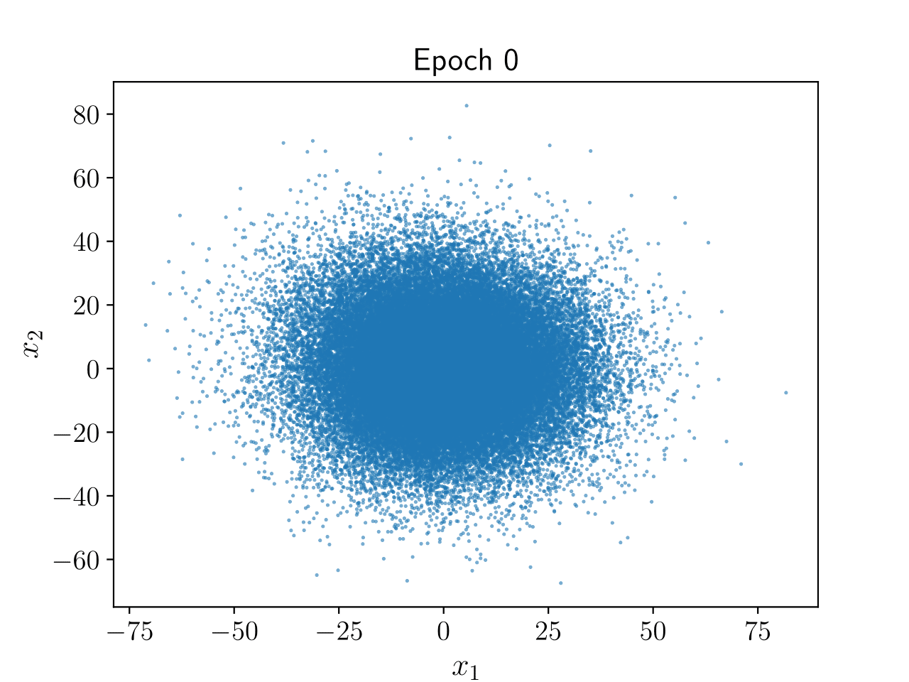
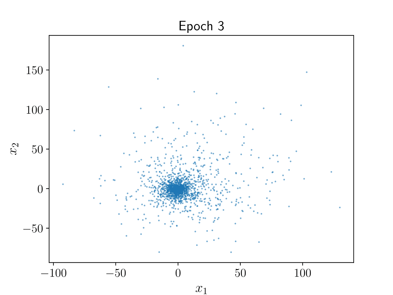
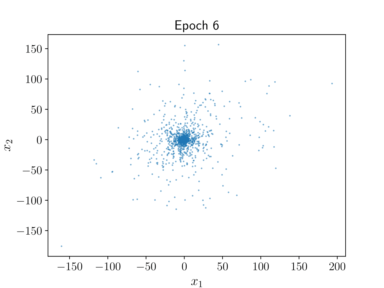
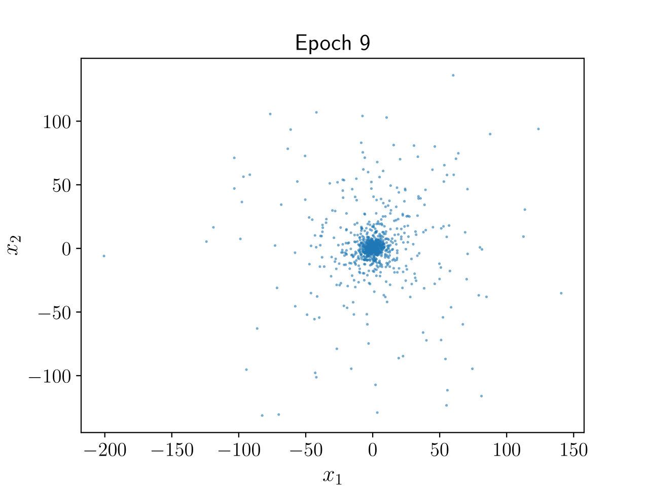
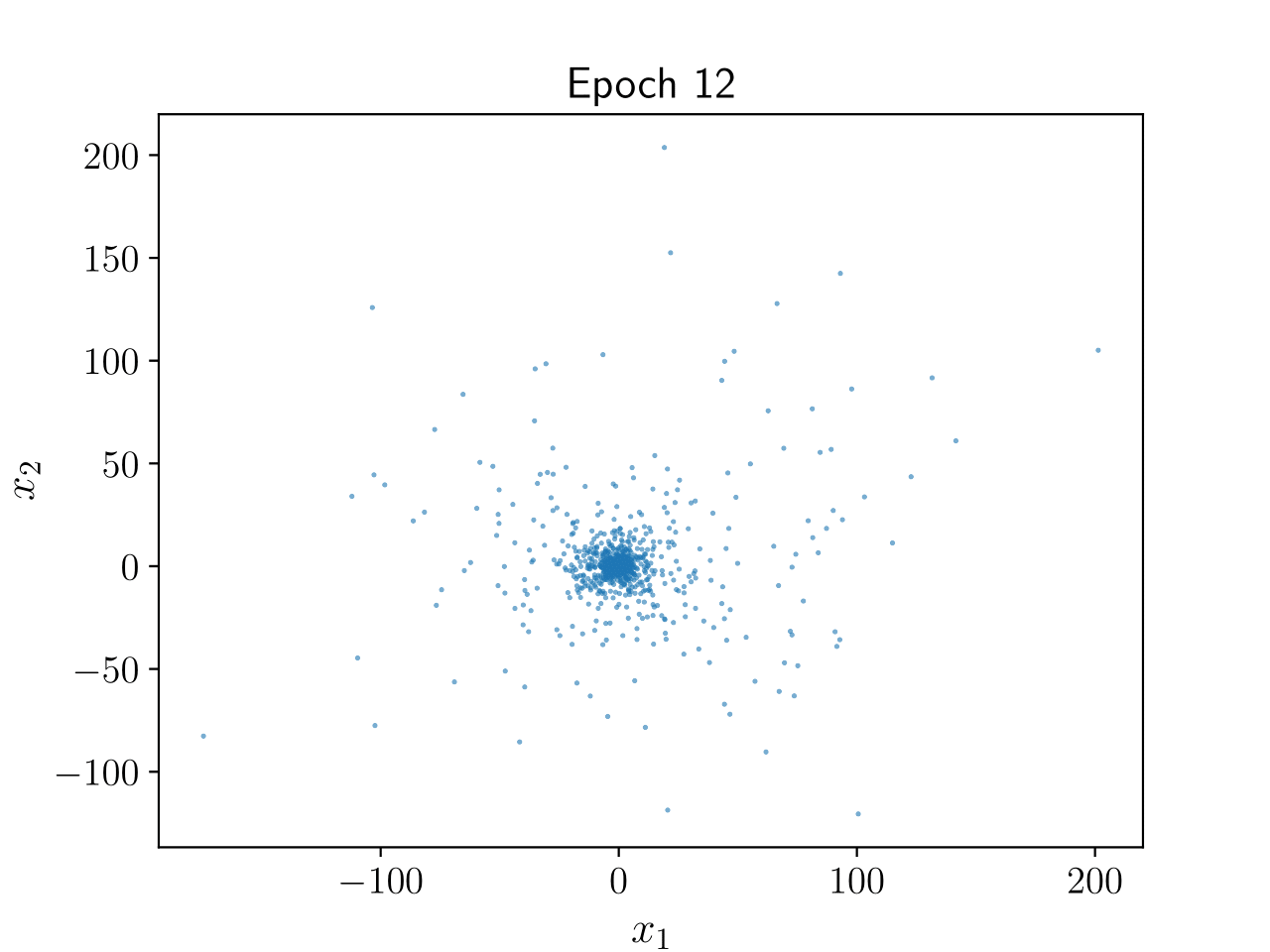
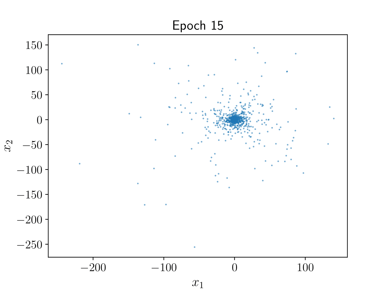
Figure 1: Random projections of per-sample gradients across epochs.

Nonlinearity Comparison.

In this set of experiments, we compare the performance of multiple nonlinear SGD methods across different metrics, using a toy example. We consider a quadratic problem $f({\mathbf{x}})=\frac{1}{2}{\mathbf{x}}^{\top}A{\mathbf{x}}+\mathbf{b}^{\top}{\mathbf{x}}$, where $A\in\mathbb{R}^{d\times d}$ is positive definite and $\mathbf{b}\in\mathbb{R}^{d}$ is fixed. We set $d=100$. The stochastic noise is generated according to the PDF from Example 1, with $\alpha=2.05$. We compare the performance of sign, component-wise and joint clipped SGD, with all three using the step-size schedule $\alpha_{t}=\frac{1}{t+1}$. We choose the clipping thresholds $m$ and $M$ for which component-wise and joint clipping performed the best, those being $m=1$ and $M=100$. All three algorithms are initialized at the zero vector and perform $T=25000$ iterations, across $R=5000$ runs. To evaluate the performance of the methods, we use the following criteria:
1. Mean-squared error: we present the MSE of the algorithms, by evaluating the gap $\|{\mathbf{x}}^{(t)}-{\mathbf{x}}^{\star}\|^{2}$ in each iteration, averaged across all runs, i.e., the final estimator at iteration $t=1,\ldots,T$, is given by $MSE^{t}=\frac{1}{R}\sum_{r=1}^{R}\|{\mathbf{x}}^{(t)}_{r}-{\mathbf{x}}^{\star}\|^{2}$, where ${\mathbf{x}}^{(t)}_{r}$ is the $t$-th iterate in the $r$-th run, generated by the algorithms.
2. High-probability estimate: we evaluate the high-probability behaviour of the methods, as follows. We consider the events $A^{t}=\{\|{\mathbf{x}}^{(t)}-{\mathbf{x}}^{\star}\|^{2}>\varepsilon\}$, for a fixed $\varepsilon>0$. To estimate the probability of $A^{t}$, for each $t=1,\ldots,T$, we construct a Monte Carlo estimator of the empirical probability, by sampling $n=3000$ instances from the $R=5000$ runs, uniformly with replacement. We then obtain the empirical probability estimator as $\mathbb{P}_{n}(A^{t})=\frac{1}{n}\sum_{i=1}^{n}\mathbb{I}_{i}(A^{t})=\frac{1}{n}\sum_{i=1}^{n}\mathbb{I}\big{(}\{\|{\mathbf{x}}_{i}^{(t)}-{\mathbf{x}}^{\star}\|^{2}>\varepsilon\}\big{)}$, where $\mathbb{I}(\cdot)$ is the indicator function and ${\mathbf{x}}^{(t)}_{i}$ is the $i$-th Monte Carlo sample.

The results are presented in Figure 2. We can see that component-wise nonlinearities outperform joint clipping, both in terms of MSE and high-probability performance and demonstrate exponential tail decay, validating our theoretical results and further underlining the usefulness of considering a general framework beyond only clipping. Additional experiments can be found in the Appendix.

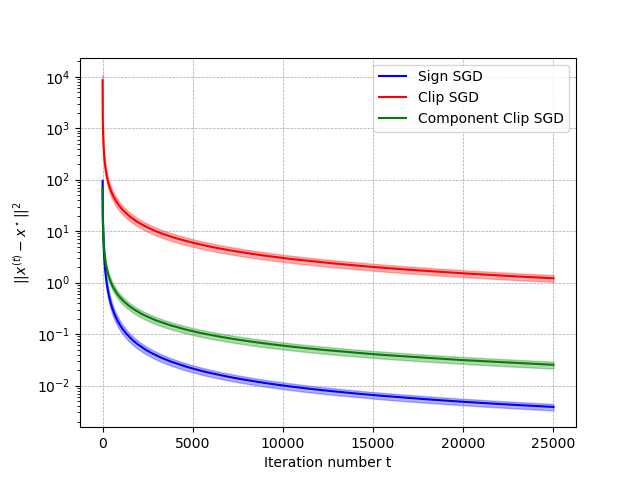
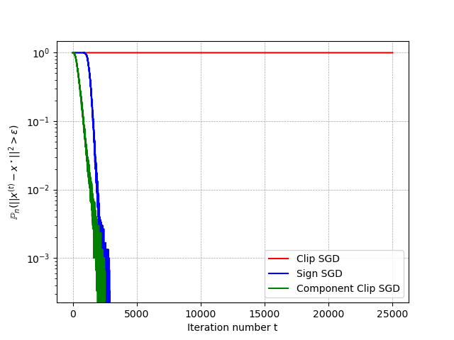
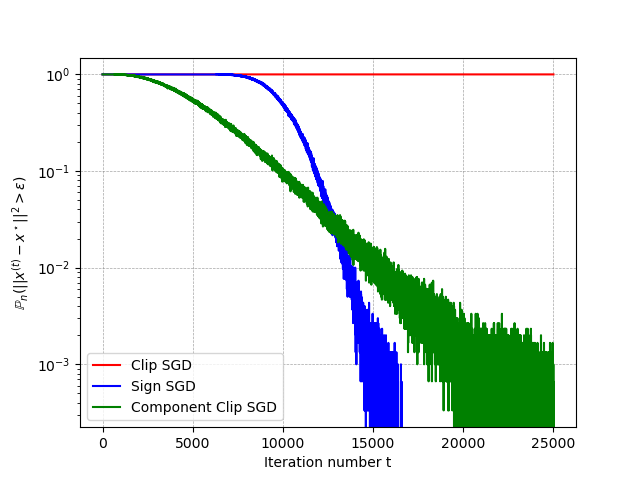
Figure 2: Performance of sign, component-wise clipping and joint clipping. Left to right: MSE performance and high-probability performance for $\varepsilon=\{0.1,0.01\}$, respectively. We can see that both component-wise nonlinearities converge faster in the MSE sense and achieve exponential tail decay. Note that clipping does not achieve exponentially decaying tails in second and third figures, as it does not reach the required accuracy in the allocated number of iterations.

5 Conclusion

We present high-probability convergence guarantees for a broad class of nonlinear SGD algorithms in the online setting and the presence of heavy-tailed noise with symmetric PDF. Our results are built on a general framework, that encompasses many popular versions of nonlinear SGD, such as clipped, normalized, quantized and sign SGD, providing high-probability convergence guarantees for both non-convex and strongly convex functions. We establish near-optimal $\widetilde{\mathcal{O}}(t^{-\nicefrac{{1}}{{4}}})$ convergence rates for non-convex costs, and similar rates for the weighted average of iterates for strongly convex costs. Additionally, for the last iterate of strongly convex costs we establish convergence at a rate $\mathcal{O}(t^{-\zeta})$, where $\zeta\in(0,1)$ depends on noise and other problem parameters. We extend our analysis beyond noises with symmetric PDF, showing convergence to a neighbourhood of stationarity for noises that are mixtures of symmetric and non-symmetric components, where the size of the neighborhood depends on choice of nonlinearity, noise and mixture coefficient. Compared to state-of-the-art works Nguyen et al., 2023a ; Sadiev et al., (2023), we extend the high-probability convergence guarantees to a broad class of nonlinearities, relax the noise moment condition, and demonstrate regimes in which our convergence rates are strictly better. This is made possible by a novel result on the interplay between the “denoised” nonlinearity and the true gradient. Numerical results confirm the presence of noise symmetry in models such as deep learning and demonstrate that clipping, exclusively considered in prior works, is not always the optimal choice of nonlinearity, further highlighting the importance and usefulness of our general framework.

Appendix A Introduction

The Appendix presents results omitted from the main body. Section B provides some useful facts and results used in the proofs, Section C provides the proofs omitted from the main body, Section D specializes the rate exponent $\zeta$ from Theorem 2 for component-wise and joint nonlinearities, Section E details the derivations for Examples 5-7, while Section F provides additional experiments.

Appendix B Useful Facts

In this section we present some useful facts and results, concerning $L$-smooth, $\mu$-strongly functions, bounded random vectors and the behaviour of nonlinearities.

Fact 1.

Let $f:\mathbb{R}^{d}\mapsto\mathbb{R}$ be $L$-smooth, $\mu$-strongly convex, and let ${\mathbf{x}}^{\star}=\operatorname*{arg\,min}_{{\mathbf{x}}\in\mathbb{R}^{d}}f({\mathbf{x}})$. Then, for any ${\mathbf{x}}\in\mathbb{R}^{d}$, we have

$$2\mu\left(f({\mathbf{x}})-f({\mathbf{x}}^{\star})\right)\leq\|\nabla f({\mathbf{x}})\|^{2}\leq 2L\left(f({\mathbf{x}})-f({\mathbf{x}}^{\star})\right).$$

Proof.

The proof of the upper bound follows by plugging $y={\mathbf{x}}$, $x={\mathbf{x}}^{\star}$ in equation (2.1.10) of Theorem 2.1.5 from Nesterov, (2018). The proof of the lower bound similarly follows by plugging $y={\mathbf{x}}$, $x={\mathbf{x}}^{\star}$ in equation (2.1.24) of Theorem 2.1.10 from Nesterov, (2018). ∎

Fact 2.

Let $X\in\mathbb{R}^{d}$ be a zero-mean, bounded random vector, i.e., $\mathbb{E}X=0$ and $\|X\|\leq\sigma$, for some $\sigma>0$. Then, $X$ is sub-Gaussian, i.e., there exists a positive constant $N=N(\sigma)$ such that, for any $v\in\mathbb{R}^{d}$, we have

$$\mathbb{E}e^{\langle X,v\rangle}\leq e^{\frac{N\|v\|^{2}}{2}}.$$

Proof.

We begin by first showing that a scalar Rademacher random variable is sub-Gaussian. Recall that a random variable $\varepsilon$ is a Rademacher random variable, if $\varepsilon$ takes the values $-1$ and $1$, both with probability $1/2$. We then have, for any $t\in\mathbb{R}$

$$\mathbb{E}e^{\varepsilon t}\stackrel{{\scriptstyle(a)}}{{=}}\frac{1}{2}\left(e^{t}+e^{-t}\right)\stackrel{{\scriptstyle(b)}}{{=}}\sum_{k=0}^{\infty}\frac{t^{2k}}{{(2k)!}}\stackrel{{\scriptstyle(c)}}{{\leq}}\sum_{k=0}^{\infty}\frac{t^{2k}}{2^{k}k!}=\sum_{k=0}^{\infty}\frac{(\nicefrac{{t^{2}}}{{2}})^{k}}{k!}=e^{\frac{t^{2}}{2}},$$ (5)

where $(a)$ follows from the definition of the Rademacher random variable, $(b)$ follows from the fact that $e^{t}=\sum_{k=0}^{\infty}\frac{t^{k}}{k!}$, for any $t\in\mathbb{R}$, while $(c)$ follows from the fact that $2k!\geq 2^{k}k!$, for any $k\in\mathbb{N}$. Let $X^{\prime}\in\mathbb{R}^{d}$ be an independent, identically distributed copy of $X$. We then have, for any $\lambda\in\mathbb{R}^{d}$

$$\mathbb{E}e^{\langle X,\lambda\rangle}\stackrel{{\scriptstyle(a)}}{{=}}\mathbb{E}e^{\langle X-\mathbb{E}X^{\prime},\lambda\rangle}\stackrel{{\scriptstyle(b)}}{{\leq}}\mathbb{E}_{X,X^{\prime}}e^{\langle X-X^{\prime},\lambda\rangle} \stackrel{{\scriptstyle(c)}}{{=}}\mathbb{E}_{X,X^{\prime}}\mathbb{E}_{\varepsilon}e^{\varepsilon\langle X-X^{\prime},\lambda\rangle}\stackrel{{\scriptstyle(d)}}{{\leq}}\mathbb{E}_{X,X^{\prime}}e^{\frac{\left(\langle X-X^{\prime},\lambda\rangle\right)^{2}}{2}}$$

$$\leq\mathbb{E}_{X,X^{\prime}}e^{\frac{\|X-X^{\prime}\|^{2}\|\lambda\|^{2}}{2}}\stackrel{{\scriptstyle(e)}}{{\leq}}e^{2\sigma^{2}\|\lambda\|^{2}},$$

where $(a)$ follows from the fact that $X$ is zero-mean, in $(b)$ we use Jensen’s inequality, $(c)$ uses the fact that $X,X^{\prime}$ are i.i.d., therefore $X-X^{\prime}$ has the same distribution as $\varepsilon(X-X^{\prime})$, where $\varepsilon$ is a Rademacher random variable, in $(d)$ we use (5), while $(e)$ follows from the boundedness of $X$. Choosing $N=4\sigma^{2}$, the desired inequality follows. ∎

Appendix C Missing Proofs

In this section we provide proofs omitted from the main body. Subsection C.1 proves results pertinent to Theorem 1, Subsection C.2 proves results relating to Theorem 2, while Subsection C.3 proves Theorem 3.

C.1 Proof of Theorem 1

In this section we prove Lemmas 3.1, 3.2, Theorem 1 and Corollary 1. We begin by proving Lemma 3.1.

Proof of Lemma 3.1.

Recall the definition of the error vector ${\mathbf{e}^{(t)}}\triangleq\boldsymbol{\Phi}^{(t)}-\boldsymbol{\Psi}^{(t)}$, where ${\boldsymbol{\Phi}}^{(t)}\triangleq\mathbb{E}_{\mathbf{z}^{(t)}}\left[{\boldsymbol{\Psi}}(\nabla f({\mathbf{x}^{(t)}})+{\mathbf{z}^{(t)}})\>|\>\mathcal{F}_{t}\right]$ is the denoised version of ${\boldsymbol{\Psi}}^{(t)}$. By definition, it then follows that

$$\mathbb{E}\left[{\mathbf{e}^{(t)}}|\>\mathcal{F}_{t}\right]=\mathbb{E}\left[{\boldsymbol{\Phi}}^{(t)}-{\boldsymbol{\Psi}}^{(t)}|\>\mathcal{F}_{t}\right]={\boldsymbol{\Phi}}^{(t)}-\mathbb{E}\left[{\boldsymbol{\Psi}}^{(t)}|\>\mathcal{F}_{t}\right]=0.$$

Moreover, by Assumption 1, we have $\|{\mathbf{e}^{(t)}}\|=\|{\boldsymbol{\Phi}}^{(t)}-{\boldsymbol{\Psi}}^{(t)}\|\leq\|{\boldsymbol{\Phi}}^{(t)}\|+\|{\boldsymbol{\Psi}}^{(t)}\|\leq\mathbb{E}\|{\boldsymbol{\Psi}}^{(t)}\|+C\leq 2C$, which proves the first claim. The second claim readily follows by using the fact that ${\mathbf{e}^{(t)}}$ is a bounded random variable and applying Fact 2. ∎

Prior to proving Lemma 3.2, we state two results used in the proof. The first result, due to Polyak and Tsypkin, (1979), provides some properties of the mapping ${\boldsymbol{\Phi}}$ for component-wise nonlinearities under symmetric noise.

Lemma C.1.

Let Assumptions 1 and 4 hold, with the nonlinearity ${\boldsymbol{\Psi}}:\mathbb{R}^{d}\mapsto\mathbb{R}^{d}$ being component wise, i.e., of the form ${\boldsymbol{\Psi}}({\mathbf{x}})=\begin{bmatrix}\mathcal{N}_{1}(x_{1}),\ldots,\mathcal{N}_{1}(x_{d})\end{bmatrix}^{\top}$. Then, the function ${\boldsymbol{\Phi}}:\mathbb{R}^{d}\mapsto\mathbb{R}^{d}$ is of the form ${\boldsymbol{\Phi}}({\mathbf{x}})=\begin{bmatrix}\phi_{1}(x_{1}),\ldots,\phi_{d}(x_{d})\end{bmatrix}^{\top}$, where $\phi_{i}(x_{i})=\mathbb{E}_{z_{i}}\left[\mathcal{N}_{1}(x_{i}+z_{i})\right]$ is the marginal expectation of the $i$-th noise component, $i\in[d]$, with the following properties:
1. $\phi_{i}$ is non-decreasing and odd, with $\phi_{i}(0)=0$;
2. $\phi_{i}$ is differentiable in zero, with $\phi_{i}^{\prime}(0)>0$.

The second result, due to Jakovetić et al., (2023), gives a useful property of ${\boldsymbol{\Phi}}$ for joint nonlinearities.

Lemma C.2.

Let Assumption 1 hold, with the nonlinearity ${\boldsymbol{\Psi}}:\mathbb{R}^{d}\mapsto\mathbb{R}^{d}$ being joint, i.e., of the form ${\boldsymbol{\Psi}}({\mathbf{x}})={\mathbf{x}}\mathcal{N}_{2}(\|{\mathbf{x}}\|)$. Then for any ${\mathbf{x}},{\mathbf{z}}\in\mathbb{R}^{d}$ such that $\|{\mathbf{z}}\|>\|{\mathbf{x}}\|$

$$\left|\mathcal{N}_{2}(\|{\mathbf{x}}+{\mathbf{z}}\|)-\mathcal{N}_{2}(\|{\mathbf{x}}-{\mathbf{z}}\|)\right|\leq\nicefrac{{\|{\mathbf{x}}\|}}{{\|{\mathbf{z}}\|}}\left[\mathcal{N}_{2}(\|{\mathbf{x}}+{\mathbf{z}}\|)+\mathcal{N}_{2}(\|{\mathbf{x}}-{\mathbf{z}}\|)\right].$$

Define $\phi^{\prime}(0)\triangleq\min_{i\in[d]}\phi_{i}^{\prime}(0)$ and $p_{0}\triangleq P(\mathbf{0})$. We are now ready to prove Lemma 3.2. For convenience, we restate the full lemma below.

Lemma C.3.

Let Assumptions 1 and 4 hold. Then, for any ${\mathbf{x}}\in\mathbb{R}^{d}$, we have $\langle{\boldsymbol{\Phi}}({\mathbf{x}}),{\mathbf{x}}\rangle\geq\min\left\{\eta_{1}\|{\mathbf{x}}\|,\eta_{2}\|{\mathbf{x}}\|^{2}\right\}$, where $\eta_{1},\eta_{2}>0$, are noise, nonlinearity and problem dependent constants. In particular, if the nonlinearity ${\boldsymbol{\Psi}}$ is component-wise, we have $\eta_{1}=\nicefrac{{\phi^{\prime}(0)\xi}}{{2\sqrt{d}}}$ and $\eta_{2}=\nicefrac{{\phi^{\prime}(0)}}{{2d}}$, where $\xi>0$ is a constant that depends only on the noise and choice of nonlinearity. If ${\boldsymbol{\Psi}}$ is a joint nonlinearity, then $\eta_{1}=p_{0}\mathcal{N}_{2}(1)/2$ and $\eta_{2}=p_{0}\mathcal{N}_{2}(1)$.

Proof of Lemma C.3.

First, consider the case when ${\boldsymbol{\Phi}}({\mathbf{x}})=[\mathcal{N}_{1}(x_{1}),\ldots,\mathcal{N}_{d}(x_{d})]^{\top}$ is component-wise. From Lemma C.1 it follows that, for any $x\in\mathbb{R}$, and any $i\in[d]$, we have

$$\phi_{i}(x)=\phi_{i}(0)+\phi_{i}^{\prime}(0)x+h_{i}(x)x=\phi_{i}^{\prime}(0)x+h_{i}(x)x,$$

where $h_{i}:\mathbb{R}\mapsto\mathbb{R}$ is such that $\lim_{x\rightarrow 0}h_{i}(x)=0$. Recalling that $\phi^{\prime}(0)=\min_{i\in[d]}\phi_{i}^{\prime}(0)>0$, it follows that there exists a $\xi>0$ (depending only on the nonlinearity $\mathcal{N}_{1}$) such that, for each $x\in\mathbb{R}$ and all $i\in[d]$, we have $|h_{i}(x)|\leq\phi^{\prime}(0)/2$, if $|x|\leq\xi$. Therefore, for any $0\leq x\leq\xi$, we have $\phi_{i}(x)\geq\frac{\phi^{\prime}(0)x}{2}$. On the other hand, for $x>\xi$, since $\phi_{i}$ is non-decreasing, we have from the previous relation that $\phi_{i}(x)\geq\phi_{i}(\xi)\geq\frac{\phi^{\prime}(0)\xi}{2}$. Therefore, it follows that $\phi_{i}(x)\geq\frac{\phi^{\prime}(0)}{2}\min\{x,\xi\}$, for any $x\geq 0$. Combined with the oddity of $\phi_{i}$, we get $x\phi_{i}(x)=|x|\phi_{i}(|x|)\geq\frac{\phi^{\prime}(0)}{2}\min\{\xi|x|,x^{2}\}$, for any $x\in\mathbb{R}$. Using the previously established relations, we then have, for any vector ${\mathbf{x}}\in\mathbb{R}^{d}$

$$\langle{\mathbf{x}},{\boldsymbol{\Phi}}({\mathbf{x}})\rangle =\sum_{i=1}^{d}x_{i}\phi_{i}(x_{i})=\sum_{i=1}^{d}|x_{i}|\phi(|x_{i}|)\geq\max_{i\in[d]}|x_{i}|\phi_{i}(|x_{i}|)\geq\frac{\phi^{\prime}(0)}{2}\max_{i\in[d]}\min\{\xi|x_{i}|,|x_{i}|^{2}\}$$

$$=\frac{\phi^{\prime}(0)}{2}\min\{\xi\|{\mathbf{x}}\|_{\infty},\|{\mathbf{x}}\|_{\infty}^{2}\}\geq\frac{\phi^{\prime}(0)}{2}\min\{\nicefrac{{\xi\|{\mathbf{x}}\|}}{{\sqrt{d}}},\nicefrac{{\|{\mathbf{x}}\|^{2}}}{{d}}\},$$ (6)

where the last inequality follows from the fact that $\|{\mathbf{x}}\|_{\infty}\geq\|{\mathbf{x}}\|/\sqrt{d}$. Next, consider the case when ${\boldsymbol{\Phi}}({\mathbf{x}})={\mathbf{x}}\mathcal{N}_{2}(\|{\mathbf{x}}\|)$ is joint. The proof follows a similar idea to the one in (Jakovetić et al.,, 2023, Lemma 6.2), with some important differences due to the different noise assumption. Fix an arbitrary ${\mathbf{x}}\in\mathbb{R}^{d}\setminus\{\mathbf{0}\}$. By the definition of ${\boldsymbol{\Psi}}$, we have

$$\langle{\boldsymbol{\Phi}}({\mathbf{x}}),{\mathbf{x}}\rangle=\int_{{\mathbf{z}}\in\mathbb{R}^{d}}\underbrace{({\mathbf{x}}+{\mathbf{z}})^{\top}{\mathbf{x}}\mathcal{N}_{2}(\|{\mathbf{x}}+{\mathbf{z}}\|)}_{\triangleq M({\mathbf{x}},{\mathbf{z}})}P({\mathbf{z}})d{\mathbf{z}}=\int_{\{{\mathbf{z}}\in\mathbb{R}^{d}:\langle{\mathbf{z}},{\mathbf{x}}\rangle\geq 0\}\cup\{{\mathbf{z}}\in\mathbb{R}^{d}:\langle{\mathbf{z}},{\mathbf{x}}\rangle<0\}}M({\mathbf{x}},{\mathbf{z}})P({\mathbf{z}})d{\mathbf{z}}.$$

Next, by the symmetry of $P$, it readily follows that $\langle{\boldsymbol{\Phi}}({\mathbf{x}}),{\mathbf{x}}\rangle=\int_{J_{1}({\mathbf{x}})}M_{2}({\mathbf{x}},{\mathbf{z}})P({\mathbf{z}})d{\mathbf{z}},$ where $J_{1}({\mathbf{x}})\triangleq\{{\mathbf{z}}\in\mathbb{R}^{d}:\langle{\mathbf{z}},{\mathbf{x}}\rangle\geq 0\}$ and $M_{2}({\mathbf{x}},{\mathbf{z}})=(\|{\mathbf{x}}\|^{2}+\langle{\mathbf{z}},{\mathbf{x}}\rangle)\mathcal{N}_{2}(\|{\mathbf{x}}+{\mathbf{z}}\|)+(\|{\mathbf{x}}\|^{2}-\langle{\mathbf{z}},{\mathbf{x}}\rangle)\mathcal{N}_{2}(\|{\mathbf{x}}-{\mathbf{z}}\|)$. Consider the set $J_{2}({\mathbf{x}})\triangleq\left\{{\mathbf{z}}\in\mathbb{R}^{d}:\frac{\langle{\mathbf{z}},{\mathbf{x}}\rangle}{\|{\mathbf{z}}\|\|{\mathbf{x}}\|}\in[0,0.5]\right\}\cup\{\mathbf{0}\}$. Clearly $J_{2}({\mathbf{x}})\subset J_{1}({\mathbf{x}})$. Note that on $J_{1}({\mathbf{x}})$ we have $\|{\mathbf{x}}+{\mathbf{z}}\|\geq\|{\mathbf{x}}-{\mathbf{z}}\|$, which, together with the fact that $\mathcal{N}_{2}$ is non-increasing, implies

$$\mathcal{N}_{2}(\|{\mathbf{x}}-{\mathbf{z}}\|)-\mathcal{N}_{2}(\|{\mathbf{x}}+{\mathbf{z}}\|)=\left|\mathcal{N}_{2}(\|{\mathbf{x}}-{\mathbf{z}}\|)-\mathcal{N}_{2}(\|{\mathbf{x}}+{\mathbf{z}}\|)\right|,$$ (7)

for any ${\mathbf{z}}\in J_{2}({\mathbf{x}})\subset J_{1}({\mathbf{x}})$. For any ${\mathbf{z}}\in J_{2}({\mathbf{x}})$ such that $\|{\mathbf{z}}\|>\|{\mathbf{x}}\|$, we then have

$$M_{2} ({\mathbf{z}},{\mathbf{x}})=\|{\mathbf{x}}\|^{2}[\mathcal{N}_{2}(\|{\mathbf{x}}-{\mathbf{z}}\|)+\mathcal{N}_{2}(\|{\mathbf{x}}+{\mathbf{z}}\|)]-\langle{\mathbf{z}},{\mathbf{x}}\rangle[\mathcal{N}_{2}(\|{\mathbf{x}}-{\mathbf{z}}\|)-\mathcal{N}_{2}(\|{\mathbf{x}}+{\mathbf{z}}\|)]$$

$$\stackrel{{\scriptstyle(a)}}{{=}}\|{\mathbf{x}}\|^{2}[\mathcal{N}_{2}(\|{\mathbf{x}}-{\mathbf{z}}\|)+\mathcal{N}_{2}(\|{\mathbf{x}}+{\mathbf{z}}\|)]-\langle{\mathbf{z}},{\mathbf{x}}\rangle\left|\mathcal{N}_{2}(\|{\mathbf{x}}-{\mathbf{z}}\|)-\mathcal{N}_{2}(\|{\mathbf{x}}+{\mathbf{z}}\|)\right|$$

$$\stackrel{{\scriptstyle(b)}}{{\geq}}\|{\mathbf{x}}\|^{2}[\mathcal{N}_{2}(\|{\mathbf{x}}-{\mathbf{z}}\|)+\mathcal{N}_{2}(\|{\mathbf{x}}+{\mathbf{z}}\|)]-\langle{\mathbf{z}},{\mathbf{x}}\rangle\nicefrac{{\|{\mathbf{x}}\|}}{{\|{\mathbf{z}}\|}}[\mathcal{N}_{2}(\|{\mathbf{x}}-{\mathbf{z}}\|)+\mathcal{N}_{2}(\|{\mathbf{x}}+{\mathbf{z}}\|)]$$

$$\stackrel{{\scriptstyle(c)}}{{\geq}}0.5\|{\mathbf{x}}\|^{2}[\mathcal{N}_{2}(\|{\mathbf{x}}-{\mathbf{z}}\|)+\mathcal{N}_{2}(\|{\mathbf{x}}+{\mathbf{z}}\|)],$$

where $(a)$ follows from (7), $(b)$ follows from Lemma C.2, while $(c)$ follows from the definition of $J_{2}({\mathbf{x}})$. Next, consider any ${\mathbf{z}}\in J_{2}({\mathbf{x}})$, such that $0<\|{\mathbf{z}}\|\leq\|{\mathbf{x}}\|$. We have

$$M_{2} ({\mathbf{z}},{\mathbf{x}})=\|{\mathbf{x}}\|^{2}[\mathcal{N}_{2}(\|{\mathbf{x}}-{\mathbf{z}}\|)+\mathcal{N}_{2}(\|{\mathbf{x}}+{\mathbf{z}}\|)]-\langle{\mathbf{z}},{\mathbf{x}}\rangle[\mathcal{N}_{2}(\|{\mathbf{x}}-{\mathbf{z}}\|)-\mathcal{N}_{2}(\|{\mathbf{x}}+{\mathbf{z}}\|)]$$

$$\stackrel{{\scriptstyle(a)}}{{=}}\|{\mathbf{x}}\|^{2}[\mathcal{N}_{2}(\|{\mathbf{x}}-{\mathbf{z}}\|)+\mathcal{N}_{2}(\|{\mathbf{x}}+{\mathbf{z}}\|)]-\langle{\mathbf{z}},{\mathbf{x}}\rangle\left|\mathcal{N}_{2}(\|{\mathbf{x}}-{\mathbf{z}}\|)-\mathcal{N}_{2}(\|{\mathbf{x}}+{\mathbf{z}}\|)\right|$$

$$\stackrel{{\scriptstyle(b)}}{{\geq}}\|{\mathbf{x}}\|^{2}[\mathcal{N}_{2}(\|{\mathbf{x}}-{\mathbf{z}}\|)+\mathcal{N}_{2}(\|{\mathbf{x}}+{\mathbf{z}}\|)]-0.5\|{\mathbf{x}}\|^{2}\left|\mathcal{N}_{2}(\|{\mathbf{x}}-{\mathbf{z}}\|)-\mathcal{N}_{2}(\|{\mathbf{x}}+{\mathbf{z}}\|)\right|$$

$$\stackrel{{\scriptstyle(c)}}{{\geq}}0.5\|{\mathbf{x}}\|^{2}[\mathcal{N}_{2}(\|{\mathbf{x}}-{\mathbf{z}}\|)+\mathcal{N}_{2}(\|{\mathbf{x}}+{\mathbf{z}}\|)],$$

where $(a)$ again follows from (7), $(b)$ follows from the definition of $J_{2}({\mathbf{x}})$ and the fact that $0<\|{\mathbf{z}}\|\leq\|{\mathbf{x}}\|$, while $(c)$ follows from the fact that $\mathcal{N}_{2}$ is non-negative and that it holds $\left|\mathcal{N}_{2}(\|{\mathbf{x}}-{\mathbf{z}}\|)-\mathcal{N}_{2}(\|{\mathbf{x}}+{\mathbf{z}}\|)\right|\leq\mathcal{N}_{2}(\|{\mathbf{x}}-{\mathbf{z}}\|)+\mathcal{N}_{2}(\|{\mathbf{x}}+{\mathbf{z}}\|)$. Finally, if ${\mathbf{z}}=\mathbf{0}$, we have $M_{2}(\mathbf{0},{\mathbf{x}})=2\|{\mathbf{x}}\|^{2}\mathcal{N}_{2}(\|{\mathbf{x}}\|)>0.5\|{\mathbf{x}}\|^{2}[\mathcal{N}_{2}(\|{\mathbf{x}}+\mathbf{0}\|)+\mathcal{N}_{2}(\|{\mathbf{x}}-\mathbf{0}\|)]$. Therefore, for any ${\mathbf{z}}\in J_{2}({\mathbf{x}})$, we have $M_{2}({\mathbf{z}},{\mathbf{x}})\geq 0.5\|{\mathbf{x}}\|^{2}[\mathcal{N}_{2}(\|{\mathbf{x}}-{\mathbf{z}}\|)+\mathcal{N}_{2}(\|{\mathbf{x}}+{\mathbf{z}}\|)]\geq\|{\mathbf{x}}\|^{2}\mathcal{N}_{2}(\|{\mathbf{x}}\|+\|{\mathbf{z}}\|)$, where the second inequality follows from the fact that $\mathcal{N}_{2}$ is non-increasing and $\|{\mathbf{x}}\pm{\mathbf{z}}\|\leq\|{\mathbf{x}}\|+\|{\mathbf{z}}\|$. Combining everything, it readily follows that

$$\langle{\boldsymbol{\Phi}}({\mathbf{x}}),{\mathbf{x}}\rangle\geq\int_{J_{2}({\mathbf{x}})}M_{2}({\mathbf{x}},{\mathbf{z}})P({\mathbf{z}})d{\mathbf{z}}\geq\|{\mathbf{x}}\|^{2}\int_{J_{2}({\mathbf{x}})}\mathcal{N}_{2}(\|{\mathbf{x}}\|+\|{\mathbf{z}}\|)P({\mathbf{z}})d{\mathbf{z}}.$$ (8)

Define $C_{0}\triangleq\min\left\{B_{0},0.5\right\}$ and consider the set $J_{3}({\mathbf{x}})\subset J_{2}({\mathbf{x}})$, which is defined as follows $J_{3}({\mathbf{x}})\triangleq\left\{{\mathbf{z}}\in\mathbb{R}^{d}:\frac{\langle{\mathbf{z}},{\mathbf{x}}\rangle}{\|{\mathbf{z}}\|\|{\mathbf{x}}\|}\in[0,0.5],\>\|{\mathbf{z}}\|\leq C_{0}\right\}\cup\{\mathbf{0}\}$. Since $a\mathcal{N}_{2}(a)$ is non-decreasing, it follows that $\mathcal{N}_{2}(a)\geq\mathcal{N}_{2}(1)\min\left\{a^{-1},1\right\}$, for any $a>0$. For any ${\mathbf{z}}\in J_{3}({\mathbf{x}})$, it then holds that $\mathcal{N}_{2}(\|{\mathbf{z}}\|+\|{\mathbf{x}}\|)\geq\mathcal{N}_{2}(1)\min\left\{1/(\|{\mathbf{x}}\|+C_{0}),1\right\}$. Plugging in (8), we then have

$$\langle{\boldsymbol{\Phi}}({\mathbf{x}}),{\mathbf{x}}\rangle\geq\|{\mathbf{x}}\|^{2}\int_{J_{3}({\mathbf{x}})}\mathcal{N}_{2}(\|{\mathbf{x}}\|+\|{\mathbf{z}}\|)P({\mathbf{z}})d{\mathbf{z}}$$

$$\geq\|{\mathbf{x}}\|^{2}\mathcal{N}_{2}(1)\min\left\{(\|{\mathbf{x}}\|+C_{0})^{-1},1\right\}\int_{J_{3}({\mathbf{x}})}P({\mathbf{z}})d{\mathbf{z}}\geq\|{\mathbf{x}}\|^{2}\mathcal{N}_{2}(1)\min\left\{(\|{\mathbf{x}}\|+C_{0})^{-1},1\right\}p_{0}.$$ (9)

If $\|{\mathbf{x}}\|\leq C_{0}$, it follows that $\|{\mathbf{x}}\|+C_{0}\leq 2C_{0}$, therefore $\min\left\{1/(\|{\mathbf{x}}\|+C_{0}),1\right\}\geq\min\left\{1/(2C_{0}),1\right\}$, and define $\kappa\triangleq\min\left\{1/(2C_{0}),1\right\}$. If $\|{\mathbf{x}}\|\geq C_{0}$, it follows that $\|{\mathbf{x}}\|+C_{0}\leq 2\|{\mathbf{x}}\|$, therefore we have that $\min\left\{1/(\|{\mathbf{x}}\|+C_{0}),1\right\}\geq\min\left\{1/(2\|{\mathbf{x}}\|),1\right\}\geq\min\left\{1/(2\|{\mathbf{x}}\|),\kappa\right\}.$ Combining everything, we get that $\langle{\boldsymbol{\Phi}}({\mathbf{x}}),{\mathbf{x}}\rangle\geq p_{0}\mathcal{N}_{2}(1)\min\left\{\|{\mathbf{x}}\|/2,\kappa\|{\mathbf{x}}\|^{2}\right\}$. Consider the constant $\kappa=\min\left\{\nicefrac{{1}}{{(2C_{0})}},1\right\}$. If $B_{0}\geq 0.5$, it follows that $C_{0}=0.5$ and therefore $\kappa=1$. On the other hand, if $B_{0}<0.5$, it follows that $C_{0}=B_{0}$ and therefore $\kappa=\min\left\{\nicefrac{{1}}{{(2B_{0})}},1\right\}=1$, as $2B_{0}<1$. ∎

We are now ready to prove Theorem 1.

Proof of Theorem 1.

For ease of notation, let $Z_{t}\triangleq\min\{\eta_{1}\|\nabla f({\mathbf{x}^{(t)}})\|,\eta_{2}\|\nabla f({\mathbf{x}^{(t)}})\|^{2}\}$. Applying the $L$-smoothness property of $f$ and the update rule (4), to get

$$f({\mathbf{x}^{(t+1)}}) \leq f({\mathbf{x}^{(t)}})-\alpha_{t}\langle\nabla f({\mathbf{x}^{(t)}}),{{\boldsymbol{\Phi}}^{(t)}}-{\mathbf{e}^{(t)}}\rangle+\frac{\alpha_{t}^{2}L}{2}\|{\boldsymbol{\Psi}}^{(t)}\|^{2}$$

$$\leq f({\mathbf{x}^{(t)}})-\alpha_{t}Z_{t}+\alpha_{t}\langle\nabla f({\mathbf{x}^{(t)}}),{\mathbf{e}^{(t)}}\rangle+\frac{\alpha_{t}^{2}LC^{2}}{2},$$

where the second inequality follows from Lemma 3.2 and Assumption 1. Rearranging and summing up the first $t$ terms, we get

$$\sum_{k=1}^{t}\alpha_{k}Z_{k}\leq\underbrace{f({\mathbf{x}}^{(1)})-f^{\star}+\frac{LC^{2}}{2}\sum_{k=1}^{t}\alpha_{k}^{2}}_{\triangleq B_{1}}+\underbrace{\sum_{k=1}^{t}\alpha_{k}\langle\nabla f({\mathbf{x}^{(k)}}),{\mathbf{e}^{(k)}}\rangle}_{\triangleq B_{2}}.$$ (10)

Denote the left-hand side of (10) by $G_{t}$, i.e., $G_{t}\triangleq\sum_{k=1}^{t}\alpha_{k}Z_{k}$ and note that $B_{1}$ is independent of the noise, i.e., is a deterministic quantity. We then have

$$\mathbb{E}\left[\exp(G_{t})\right]\stackrel{{\scriptstyle\eqref{eq:5}}}{{\leq}}\mathbb{E}\left[\exp\left(B_{1}+B_{2}\right)\right]=\exp\left(B_{1}\right)\mathbb{E}\left[\exp(B_{2})\right].$$

We now bound $\mathbb{E}[\exp(B_{2})]$. Denote by $\mathbb{E}_{t}[\cdot]\triangleq\mathbb{E}[\cdot\>|\>\mathcal{F}_{t}]$ the expectation conditioned on history up to time $t$. We then have

$$\mathbb{E}[\exp(B_{2})] =\mathbb{E}\left[\exp\left(\sum_{k=1}^{t}\alpha_{k}\langle\nabla f({\mathbf{x}^{(k)}}),{\mathbf{e}^{(k)}}\rangle\right)\right]$$

$$=\mathbb{E}\left[\exp\left(\sum_{k=1}^{t-1}\alpha_{k}\langle\nabla f({\mathbf{x}^{(k)}}),{\mathbf{e}^{(k)}}\rangle\right)\mathbb{E}_{t}\left[\exp(\alpha_{t}\langle\nabla f({\mathbf{x}}^{(t)}),{\mathbf{e}}^{(t)}\rangle)\right]\right]$$

$$\leq\mathbb{E}\left[\exp\left(\sum_{k=1}^{t-1}\alpha_{k}\langle\nabla f({\mathbf{x}^{(k)}}),{\mathbf{e}^{(k)}}\rangle\right)\exp\left(2C^{2}\alpha_{t}^{2}\|\nabla f({\mathbf{x}}^{(t)})\|^{2}\right)\right],$$ (11)

where the last inequality follows from Lemma 3.1. Next, consider $\|\nabla f({\mathbf{x}^{(k)}})\|$, for any $k\geq 0$. Define $A_{t}\triangleq\sum_{k=1}^{t}\alpha_{k}$ and use $L$-smoothness, to get

$$\|\nabla f({\mathbf{x}^{(k)}})\| \leq L\|{\mathbf{x}^{(k)}}-{\mathbf{x}}^{\star}\|=L\|{\mathbf{x}}^{(k-1)}-\alpha_{k-1}{\boldsymbol{\Psi}}^{(k-1)}-{\mathbf{x}}^{\star}\|\leq L\left(\|{\mathbf{x}}^{(k-1)}-{\mathbf{x}}^{\star}\|+\alpha_{k-1}C\right)$$

$$\leq\ldots\leq L\left(\|{\mathbf{x}}^{(1)}-{\mathbf{x}}^{\star}\|+C\sum_{s=1}^{k-1}\alpha_{s}\right)\leq L\left(\|{\mathbf{x}}^{(1)}-{\mathbf{x}}^{\star}\|+CA_{k}\right),$$ (12)

where we recall that ${\mathbf{x}}^{\star}\in\mathcal{X}$ is any stationary point of $f$. Combining (11) and (12), we get

$$\mathbb{E}[\exp(B_{2})] \leq\exp\left(4C^{2}L^{2}D_{\mathcal{X}}\alpha_{t}^{2}+4C^{4}L^{2}\alpha_{t}^{2}A_{t}^{2}\right)\mathbb{E}\left[\exp\left(\sum_{k=1}^{t-1}\alpha_{k}\langle\nabla f({\mathbf{x}^{(k)}}),{\mathbf{e}^{(k)}}\rangle\right)\right],$$

where $D_{\mathcal{X}}=\inf_{{\mathbf{x}}^{\star}\in\mathcal{X}}\|{\mathbf{x}}^{(1)}-{\mathbf{x}}^{\star}\|^{2}$ is the distance of the initial model estimate from the set of stationary points. Repeating the same arguments recursively, we then get

$$\mathbb{E}\left[\exp(B_{2})\right]\leq\exp\left(4C^{2}L^{2}D_{\mathcal{X}}\sum_{k=1}^{t}\alpha_{k}^{2}+4C^{4}L^{2}\sum_{k=1}^{t}\alpha_{k}^{2}A_{k}^{2}\right),$$

Combining everything, we get

$$\mathbb{E}\left[\exp(G_{t})\right]\leq\exp\left(f({\mathbf{x}}^{(1)})-f^{\star}+LC^{2}\left(\nicefrac{{1}}{{2}}+4LD_{\mathcal{X}}\right)\sum_{k=1}^{t}\alpha_{k}^{2}+4C^{4}L^{2}\sum_{k=1}^{t}\alpha_{k}^{2}A_{k}^{2}\right).$$

Define $N_{t}\triangleq f({\mathbf{x}}^{(1)})-f^{\star}+LC^{2}\left(\nicefrac{{1}}{{2}}+4LD_{\mathcal{X}}\right)\sum_{k=1}^{t}\alpha_{k}^{2}+4C^{4}L^{2}\sum_{k=1}^{t}\alpha_{k}^{2}A_{k}^{2}$. Using Markov’s inequality, it then follows that, for any $\epsilon>0$

$$\mathbb{P}(G_{t}>\epsilon)\leq\exp(-\epsilon)\mathbb{E}[\exp(G_{t})]\leq\exp(-\epsilon+N_{t})\iff\mathbb{P}(G_{t}>\epsilon+N_{t})\leq\exp(-\epsilon).$$

Finally, for any $\beta\in(0,1)$, with probability at least $1-\beta$, we have

$$G_{t}\leq\log(\nicefrac{{1}}{{\beta}})+N_{t}\iff A_{t}^{-1}G_{t}\leq A_{t}^{-1}\left(\log(\nicefrac{{1}}{{\beta}})+N_{t}\right).$$ (13)

Note that for the step-size schedule $\alpha_{t}=\frac{a}{(t+1)^{\delta}}$ and any $\delta\in(\nicefrac{{2}}{{3}},1)$, using lower and upper Darboux sums, we have

$$\frac{a}{1-\delta}((t+2)^{1-\delta}-2^{1-\delta}) \leq A_{t}\leq\frac{a}{1-\delta}((t+1)^{1-\delta}-1),$$ (14)

$$\frac{a^{2}}{2\delta-1}(2^{1-2\delta}-(t+2)^{1-2\delta}) \leq\sum_{k=0}^{t-1}\alpha_{k}^{2}\leq\frac{a^{2}}{2\delta-1}(1-(t+1)^{1-2\delta}).$$

Plugging (14) in (13), we then get, with probability at least $1-\beta$

$$\sum_{k=1}^{t} \widetilde{\alpha}_{k}Z_{k}\leq\frac{(1-\delta)\left(f({\mathbf{x}}^{(1)})-f^{\star}+\log(\nicefrac{{1}}{{\beta}})\right)}{a((t+2)^{1-\delta}-2^{1-\delta})}$$

$$+\frac{a(1-\delta)LC^{2}(\nicefrac{{1}}{{2}}+4LD_{\mathcal{X}})}{(2\delta-1)((t+2)^{1-\delta}-2^{1-\delta})}+\frac{4a^{3}C^{4}L^{2}\sum_{k=1}^{t}(k+1)^{2-4\delta}}{(1-\delta)((t+2)^{1-\delta}-2^{1-\delta})}.$$ (15)

To bound the last sum, we consider different step-size schedules.

1. First, consider $\alpha_{t}=\frac{a}{(t+1)^{\delta}}$, for $\delta\in(\nicefrac{{2}}{{3}},\nicefrac{{3}}{{4}})$. Using the lower Darboux sum, we have

$$\sum_{k=1}^{t}(k+1)^{2-4\delta}\leq\int_{1}^{t+1}k^{2-4\delta}dk\leq\frac{(t+1)^{3-4\delta}}{3-4\delta}.$$

Combining with (15), we get

$$\sum_{k=1}^{t}\widetilde{\alpha}_{k}Z_{k}\leq\frac{R_{1}}{(t+2)^{1-\delta}-2^{1-\delta}}+\frac{R_{2}(t+1)^{3-4\delta}}{(t+2)^{1-\delta}-2^{1-\delta}},$$ (16)

where $R_{1}\triangleq(1-\delta)\left[\frac{\left(f({\mathbf{x}}^{(1)})-f^{\star}+\log(\nicefrac{{1}}{{\beta}})\right)}{a}+\frac{aLC^{2}(\nicefrac{{1}}{{2}}+4LD_{\mathcal{X}})}{(2\delta-1)}\right]$ and $R_{2}\triangleq\frac{4a^{3}C^{4}L^{2}}{(1-\delta)(3-4\delta)}$.

2. Next, consider $\alpha_{t}=\frac{a}{(t+1)^{\delta}}$, for $\delta=\nicefrac{{3}}{{4}}$. Using the lower Darboux sum, we have

$$\sum_{k=1}^{t}(k+1)^{2-4\delta}=\sum_{k=1}^{t}\frac{1}{(k+1)}\leq\int_{1}^{t+1}\frac{1}{k}dk\leq\log(t+1).$$

Combining with (15), we get

$$\sum_{k=1}^{t}\widetilde{\alpha}_{k}Z_{k}\leq\frac{R_{1}+R_{3}\log(t+1)}{(t+2)^{\nicefrac{{1}}{{4}}}-2^{\nicefrac{{1}}{{4}}}},$$ (17)

where $R_{3}\triangleq\frac{4a^{3}C^{4}L^{2}}{(1-\delta)}$.

3. Finally, for $\alpha_{t}=\frac{a}{(t+1)^{\delta}}$, where $\delta\in(\nicefrac{{3}}{{4}},1)$, we have

$$\sum_{k=1}^{t}(k+1)^{2-4\delta}\leq\int_{1}^{t+1}k^{2-4\delta}dk\leq\frac{1}{4\delta-3},$$

therefore, combining with (15), we get

$$\sum_{k=1}^{t}\widetilde{\alpha}_{k}Z_{k}\leq\frac{R_{1}+R_{4}}{(t+2)^{1-\delta}-2^{1-\delta}},$$ (18)

where $R_{4}\triangleq\frac{4a^{3}C^{4}L^{2}}{(1-\delta)(4\delta-3)}$.

Finally, to obtain a bound on the quantity of interest $\min_{k\in[t]}\|\nabla f({\mathbf{x}^{(k)}})\|^{2}$, we proceed as follows. Notice that the bounds in (16)-(18) can be represented in a unified manner as

$$\sum_{k=1}^{t}\widetilde{\alpha}_{k}Z_{k}\leq Mt^{-\kappa},$$ (19)

for appropriately selected constants $M,\kappa>0$. Next, define $U\triangleq\{k\in[t]:\>\|\nabla f({\mathbf{x}^{(k)}})\|\leq\eta_{1}/\eta_{2}\}$, with $U^{c}\triangleq[t]\setminus U$. From (19), we then have

$$\sum_{k\in U^{c}}\widetilde{\alpha}_{k}\|\nabla f({\mathbf{x}^{(k)}})\|\leq M_{1}t^{-\kappa}\text{ and }\sum_{k\in U}\widetilde{\alpha}_{k}\|\nabla f({\mathbf{x}^{(k)}})\|^{2}\leq M_{2}t^{-\kappa},$$

where $M_{1}=M/\eta_{1}$, $M_{2}=M/\eta_{2}$. It then readily follows that

$$\min_{k\in[t]}\|\nabla f({\mathbf{x}^{(k)}})\|\leq\sum_{k\in U}\widetilde{\alpha}_{k}\|\nabla f({\mathbf{x}^{(k)}})\|+\sum_{k\in U^{c}}\widetilde{\alpha}_{k}\|\nabla f({\mathbf{x}^{(k)}})\|\leq\sum_{k=1}^{t}\widetilde{\alpha}_{k}z_{k}+M_{1}t^{-\kappa},$$

where $z_{k}=\|\nabla f({\mathbf{x}^{(k)}})\|$, for $k\in U$, otherwise $z_{k}=0$. Using Jensen’s inequality, we get

$$\min_{k\in[t]}\|\nabla f({\mathbf{x}^{(k)}})\|\leq\sqrt{\sum_{k=1}^{t}\widetilde{\alpha}_{k}z_{k}^{2}}+M_{1}t^{-\kappa}=\sqrt{\sum_{k\in U}\widetilde{\alpha}_{k}\|\nabla f({\mathbf{x}^{(k)}})\|^{2}}+M_{1}t^{-\kappa}\leq\sqrt{M_{2}t^{-\kappa}}+M_{1}t^{-\kappa}.$$

Squaring both sides and using $(a+b)^{2}\leq 2a^{2}+2b^{2}$, gives the desired result. ∎

We next prove Corollary 1.

Proof of Corollary 1.

Recall the definition of the Huber loss function $H_{\lambda}:\mathbb{R}\mapsto[0,\infty)$, parametrized by $\lambda>0$, e.g., Huber, (1964), given by

$$H_{\lambda}(x)\triangleq\begin{cases}\frac{1}{2}x^{2},&|x|\leq\lambda,\\ \lambda|x|-\frac{\lambda^{2}}{2},&|x|>\lambda.\end{cases}$$

By the definition of Huber loss, it is not hard to see that it is a convex, non-decreasing function on $[0,\infty)$. Moreover, by the definition of Huber loss, we have, for any $k\geq 1$

$$Z_{k}=\min\{\eta_{1}\|\nabla f({\mathbf{x}^{(k)}})\|,\eta_{2}\|\nabla f({\mathbf{x}^{(k)}})\|^{2}\}\geq\eta_{2}H_{\eta_{1}/\eta_{2}}(\|\nabla f({\mathbf{x}^{(k)}})\|).$$ (20)

Next, recall that Assumption 3 implies the gradient domination property, i.e., $\|\nabla f({\mathbf{x}})\|^{2}\geq 2\mu(f({\mathbf{x}})-f^{\star})$, for any ${\mathbf{x}}\in\mathbb{R}^{d}$, see, e.g., Nesterov, (2018). Combined with the definition of strong convexity, we have $\|\nabla f({\mathbf{x}})\|\geq\mu\|{\mathbf{x}}-{\mathbf{x}}^{\star}\|$, for any ${\mathbf{x}}\in\mathbb{R}^{d}$. Combining (20) with the gradient domination property, we get

$$\sum_{k=1}^{t}\widetilde{\alpha}_{k}Z_{k}\geq\eta_{2}\sum_{k=1}^{t}\widetilde{\alpha}_{k}H_{\eta_{1}/\eta_{2}}(\mu\|{\mathbf{x}^{(k)}}-{\mathbf{x}}^{\star}\|)\geq\mu^{2}\eta_{2}H_{\eta_{1}/(\eta_{2}\mu)}(\|\widehat{{\mathbf{x}}}^{(t)}-{\mathbf{x}}^{\star}\|),$$

where $\widehat{{\mathbf{x}}}^{(t)}\triangleq\sum_{k=1}^{t}\widetilde{\alpha}_{k}{\mathbf{x}^{(k)}}$ is the weighted average of the first $t$ iterates, the first inequality follows from (20), the gradient domination property and the fact that $H$ is non-decreasing, while the second inequality follows from the fact that $H$ is convex and non-decreasing, applying Jensen’s inequality twice and noticing that $H_{\lambda}(\mu x)=\mu^{2}H_{\lambda/\mu}(x)$. Using (19), it readily follows that

$$H_{\eta_{1}/(\eta_{2}\mu)}(\|\widehat{{\mathbf{x}}}^{(t)}-{\mathbf{x}}^{\star}\|)\leq\frac{M}{\eta_{2}^{2}\mu^{2}t^{\kappa}},.$$ (21)

where $M,\kappa$ depend on the step-size schedule and other problem parameters. By the definition of Huber loss and (21), if $\|\widehat{{\mathbf{x}}}^{(t)}-{\mathbf{x}}^{\star}\|\leq\nicefrac{{\eta_{1}}}{{\eta_{2}\mu}}$, we have

$$\|\widehat{{\mathbf{x}}}^{(t)}-{\mathbf{x}}^{\star}\|^{2}\leq\frac{2M}{\eta_{2}^{2}\mu^{2}t^{\kappa}}.$$ (22)

Otherwise, if $\|\widehat{{\mathbf{x}}}^{(t)}-{\mathbf{x}}^{\star}\|>\nicefrac{{\eta_{1}}}{{\eta_{2}\mu}}$, by (21), we have

$$\frac{\eta_{1}\|\widehat{{\mathbf{x}}}^{(t)}-{\mathbf{x}}^{\star}\|}{2\eta_{2}\mu}<\frac{\eta_{1}\|\widehat{{\mathbf{x}}}^{(t)}-{\mathbf{x}}^{\star}\|}{\eta_{2}\mu}-\frac{\eta_{1}^{2}}{2\eta_{2}^{2}\mu^{2}}=H_{\eta_{1}/(\eta_{2}\mu)}(\|\widehat{{\mathbf{x}}}^{(t)}-{\mathbf{x}}^{\star}\|)\leq\frac{M}{\eta_{2}^{2}\mu^{2}t^{\kappa}},$$

implying that

$$\|\widehat{{\mathbf{x}}}^{(t)}-{\mathbf{x}}^{\star}\|^{2}\leq\frac{4M^{2}}{\eta_{1}^{2}\eta_{2}^{2}\mu^{2}t^{2\kappa}}.$$ (23)

Combining (22) and (23), it then follows that

$$\|\widehat{{\mathbf{x}}}^{(t)}-{\mathbf{x}}^{\star}\|^{2}\leq\max\left\{\frac{2M}{\eta_{2}^{2}\mu^{2}t^{\kappa}},\frac{4M^{2}}{\eta_{1}^{2}\eta_{2}^{2}\mu^{2}t^{2\kappa}}\right\},$$

completing the proof. ∎

C.2 Proof of Theorem 2

In this section we prove Lemma 3.3 and Theorem 2. In order to prove Lemma 3.3, we first state and prove some intermediate results.

Lemma C.4.

Let Assumptions 1-4 hold, with the step-size given by $\alpha_{t}=\frac{a}{(t+1)^{\delta}}$, for any $\delta\in(0.5,1)$ and $a>0$. Then, for any $t\geq 1$, we have

$$\|\nabla f({\mathbf{x}^{(t)}})\|\leq H_{t}\triangleq L\left(\|{\mathbf{x}}^{(1)}-{\mathbf{x}}^{\star}\|+aC\right)\frac{(t+1)^{1-\delta}}{1-\delta}.$$

Proof.

Using $L$-smoothness of $f$ and the update (3), we have

$$\|\nabla f({\mathbf{x}^{(t)}})\| \leq L\|{\mathbf{x}^{(t)}}-{\mathbf{x}}^{\star}\|=L\|{\mathbf{x}}^{(t-1)}-\alpha_{t-1}{\boldsymbol{\Psi}}^{(t-1)}-{\mathbf{x}}^{\star}\|$$

$$\leq L\left(\|{\mathbf{x}}^{(t-1)}-{\mathbf{x}}^{\star}\|+\alpha_{t-1}\|\boldsymbol{\Psi}^{(t-1)}\|\right)$$

$$\leq L\left(\|{\mathbf{x}}^{(t-1)}-{\mathbf{x}}^{\star}\|+\alpha_{t-1}C\right).$$ (24)

Unrolling the recursion in (24), we get

$$\|\nabla f({\mathbf{x}^{(t)}})\|\leq L\|{\mathbf{x}}^{(1)}-{\mathbf{x}}^{\star}\|+LC\sum_{k=1}^{t}\alpha_{k}\leq L\left(\|{\mathbf{x}}^{(1)}-{\mathbf{x}}^{\star}\|+aC\right)\frac{(t+1)^{1-\delta}}{1-\delta},$$

completing the proof. ∎

The next result characterizes the behaviour of the nonlinearity, when it takes the form ${\boldsymbol{\Psi}}({\mathbf{x}})=\left[\mathcal{N}_{1}(x_{1}),\dots,\mathcal{N}_{1}(x_{d})\right]^{\top}$. It follows a similar idea to Lemma 5.5 from Jakovetić et al., (2023), with the main difference due to allowing for potentially different marginal PDFs of each noise component. Since the proof follows the same steps, we omit it for brevity.

Lemma C.5.

Let Assumptions 1-4 hold and the nonlinearity ${\boldsymbol{\Psi}}$ be component-wise, i.e., of the form ${\boldsymbol{\Psi}}({\mathbf{x}})=\left[\mathcal{N}_{1}(x_{1}),\dots,\mathcal{N}_{1}(x_{d})\right]^{\top}$. Then, there exists a positive constant $\xi$ such that, for any $t\geq 1$, there holds almost surely for each $j=1,\ldots,d$, that $|\phi^{(t)}_{i}|\geq|[\nabla f({\mathbf{x}^{(t)}})]_{i}|\frac{\phi_{i}^{\prime}(0)\xi}{2H_{t}}$, where $H_{t}$ is defined in Lemma C.4, while $\phi_{i}^{\prime}(0)=\frac{\partial}{\partial x_{i}}\mathbb{E}_{z_{i}}\mathcal{N}_{1}(x_{i}+z_{i})\>\big{|}_{x_{i}=0}$.

The next result characterizes the behaviour of the nonlinearity, when it takes the form ${\boldsymbol{\Psi}}({\mathbf{x}})={\mathbf{x}}\mathcal{N}_{2}(\|{\mathbf{x}}\|)$.

Lemma C.6.

Let Assumptions 1-4 hold and the nonlinearity be of the form ${\boldsymbol{\Psi}}({\mathbf{x}})={\mathbf{x}}\mathcal{N}_{2}(\|{\mathbf{x}}\|)$. Then, for any $t\geq 1$, there holds almost surely that

$$\langle\nabla f({\mathbf{x}^{(t)}}),\boldsymbol{\Phi}^{(t)}\rangle\geq\frac{\|\nabla f({\mathbf{x}^{(t)}})\|^{2}p_{0}\mathcal{N}_{2}(1)}{H_{t}+C_{0}},$$

where $p_{0}=P(\mathbf{0})$, $C_{0}=\min\{0.5,B_{0}\}$ and $H_{t}$ is defined in Lemma C.4.

Proof.

We start from (9), which tells us that, for any $t\geq 1$, almost surely

$$\langle{{\boldsymbol{\Phi}}^{(t)}},\nabla f({\mathbf{x}^{(t)}})\rangle\geq\|\nabla f({\mathbf{x}^{(t)}})\|^{2}p_{0}\mathcal{N}_{2}(1)\min\left\{\frac{1}{\|\nabla f({\mathbf{x}^{(t)}})\|+C_{0}},1\right\}.$$

Combining with Lemma C.4 and the fact that $H_{t}\geq 1$, we get almost surely

$$\langle{{\boldsymbol{\Phi}}^{(t)}},\nabla f({\mathbf{x}^{(t)}})\rangle\geq\frac{\|\nabla f({\mathbf{x}^{(t)}})\|^{2}p_{0}\mathcal{N}_{2}(1)}{H_{t}+C_{0}},$$

which completes the proof. ∎

We are now ready to prove Lemma 3.3.

Proof of Lemma 3.3.

First, consider the case when the nonlinearity is of the form ${\boldsymbol{\Psi}}({\mathbf{x}})=\left[\mathcal{N}_{1}(x_{1}),\dots,\mathcal{N}_{1}(x_{d})\right]^{\top}$. We then have

$$\langle{{\boldsymbol{\Phi}}^{(t)}},\nabla f({\mathbf{x}^{(t)}})\rangle =\sum_{i=1}^{d}\phi^{(t)}_{i}[\nabla f({\mathbf{x}^{(t)}})]_{i}\stackrel{{\scriptstyle(a)}}{{=}}\sum_{i=1}^{d}|\phi^{(t)}_{i}||[\nabla f({\mathbf{x}^{(t)}})]_{i}|$$

$$\stackrel{{\scriptstyle(b)}}{{\geq}}\sum_{i=1}^{d}|[\nabla f({\mathbf{x}^{(t)}})]_{i}|^{2}\frac{\phi_{i}^{\prime}(0)\xi}{2H_{t}}\stackrel{{\scriptstyle(c)}}{{\geq}}\frac{\phi^{\prime}(0)\xi}{2H_{t}}\|\nabla f({\mathbf{x}^{(t)}})\|^{2}=\gamma(t+1)^{\delta-1}\|\nabla f({\mathbf{x}^{(t)}})\|^{2},$$

where $\gamma=\frac{(1-\delta)\phi^{\prime}(0)\xi}{2L\left(\|{\mathbf{x}}^{(1)}-{\mathbf{x}}^{\star}\|+aC\right)}$, $(a)$ follows from the oddity of $\mathcal{N}_{1}$, $(b)$ follows from Lemma C.5, $(c)$ follows from $\phi^{\prime}(0)=\min_{i=1,\ldots,d}\phi_{i}^{\prime}(0)$. On the other hand, if the nonlinearity is of the form ${\boldsymbol{\Psi}}({\mathbf{x}})={\mathbf{x}}\mathcal{N}_{2}(\|{\mathbf{x}}\|)$, we get

$$\langle{{\boldsymbol{\Phi}}^{(t)}},\nabla f({\mathbf{x}^{(t)}})\rangle\geq\frac{p_{0}\mathcal{N}_{2}(1)\|\nabla f({\mathbf{x}^{(t)}})\|^{2}}{H_{t}+C_{0}}\geq\gamma(t+1)^{\delta-1}\|\nabla f({\mathbf{x}^{(t)}})\|^{2},$$

where $\gamma=\frac{(1-\delta)p_{0}\mathcal{N}_{2}(1)}{L\left(\|{\mathbf{x}}^{(1)}-{\mathbf{x}}^{\star}\|+aC\right)+C_{0}}$, the first inequality follows from Lemma C.6, while the second follows from the definition of $H_{t}$ and the fact that $H_{t}+C_{0}\leq(L\left(\|{\mathbf{x}}^{(1)}-{\mathbf{x}}^{\star}\|+aC\right)+C_{0})\frac{(t+1)^{1-\delta}}{1-\delta}$. This completes the proof. ∎

We next prove Theorem 2.

Proof of Theorem 2.

Using $L$-smoothness of $f$, the update rule (4) and Lemma 3.3, we have

$$f({\mathbf{x}^{(t+1)}}) \leq f({\mathbf{x}^{(t)}})-\alpha_{t}\langle\nabla f({\mathbf{x}^{(t)}}),{\boldsymbol{\Phi}}^{(t)}-{\mathbf{e}^{(t)}}\rangle+\mfrac{\alpha_{t}^{2}L}{2}\|\boldsymbol{\Psi}^{(t)}\|$$

$$\leq f({\mathbf{x}^{(t)}})-\mfrac{a\gamma\|\nabla f({\mathbf{x}^{(t)}})\|^{2}}{(t+1)}+\mfrac{a\langle\nabla f({\mathbf{x}^{(t)}}),{\mathbf{e}^{(t)}}\rangle}{(t+1)^{\delta}}+\mfrac{a^{2}LC^{2}}{2(t+1)^{2\delta}}.$$

Subtracting $f^{\star}$ from both sides of the inequality, defining $F^{(t)}=f({\mathbf{x}^{(t)}})-f^{\star}$ and using $\mu$-strong convexity of $f$, we get

$$F^{(t+1)}\leq\left(1-\mfrac{2\mu a\gamma}{t+1}\right)F^{(t)}+\mfrac{a\langle\nabla f({\mathbf{x}^{(t)}}),{\mathbf{e}^{(t)}}\rangle}{(t+1)^{\delta}}+\mfrac{a^{2}LC^{2}}{2(t+1)^{2\delta}}.$$ (25)

Let $\zeta=\min\left\{2\delta-1,\nicefrac{{a\gamma\mu}}{{2}}\right\}$. Defining $Y^{(t)}\triangleq t^{\zeta}F^{(t)}=t^{\zeta}(f({\mathbf{x}^{(t)}})-f^{\star})$, from (25) we get

$$Y^{(t+1)}\leq a_{t}Y^{(t)}+b_{t}\langle\nabla f({\mathbf{x}^{(t)}}),{\mathbf{e}^{(t)}}\rangle+c_{t}V,$$ (26)

where $a_{t}=\left(1-\frac{2\mu a\gamma}{t+1}\right)\left(\frac{t+1}{t}\right)^{\zeta}$, $b_{t}=\frac{a}{(t+1)^{\delta-\zeta}}$, $c_{t}=\frac{a^{2}}{(t+1)^{2\delta-\zeta}}$ and $V=\frac{LC^{2}}{2}$. Denote the MGF of $Y^{(t)}$ conditioned on $\mathcal{F}_{t}$ as $M_{t+1|t}(\nu)=\mathbb{E}\left[\exp\left(\nu Y^{(t+1)}\right)|\mathcal{F}_{t}\right]$. We then have, for any $\nu\geq 0$

$$M_{t+1|t}(\nu) \overset{(a)}{\leq}\mathbb{E}\left[\exp\left(\nu(a_{t}Y^{(t)}+b_{t}\langle{\mathbf{e}^{(t)}},\nabla f({\mathbf{x}^{(t)}})\rangle+c_{t}V)\right)\big{|}\>\mathcal{F}_{t}\right]$$

$$\overset{(b)}{\leq}\exp(\nu a_{t}Y^{(t)}+\nu c_{t}V)\mathbb{E}\left[\exp(\nu b_{t}\langle{\mathbf{e}^{(t)}},\nabla f({\mathbf{x}^{(t)}})\rangle)\big{|}\>\mathcal{F}_{t}\right]$$

$$\overset{(c)}{\leq}\exp\left(\nu a_{t}Y^{(t)}+\nu c_{t}V+\nu^{2}b^{2}_{t}N\|\nabla f({\mathbf{x}^{(t)}})\|^{2}\right)$$

$$\overset{(d)}{\leq}\exp\left(\nu a_{t}Y^{(t)}+\nu c_{t}V+2\nu^{2}b_{t}^{\prime 2}LNY^{(t)}\right),$$ (27)

where $(a)$ follows from (26), $(b)$ follows from the fact that $Y^{(t)}$ is $\mathcal{F}_{t}$ measurable, $(c)$ follows from Lemma 3.1, in $(d)$ we use $\|\nabla f({\mathbf{x}})\|^{2}\leq 2L(f({\mathbf{x}})-f^{\star})$ and define $b^{\prime}_{t}=a\frac{t^{\frac{-\zeta}{2}}}{(t+1)^{\delta-\zeta}}$, so that $b_{t}=t^{\frac{\zeta}{2}}b^{\prime}_{t}$. For the choice $0\leq\nu\leq B$, for some $B>0$ (to be specified later), we get

$$M_{t+1|t}(\nu)\leq\exp\left(\nu(a_{t}+2b_{t}^{\prime 2}LNB)Y^{(t)}\right)\exp\left(\nu c_{t}V\right).$$

Taking the full expectation, we get

$$M_{t+1}(\nu)\leq M_{t}((a_{t}+2b_{t}^{\prime 2}LNB)\nu)\exp(\nu c_{t}V).$$ (28)

Similarly to the approach in Harvey et al., (2019), we now want to show that $M_{t}(\nu)\leq e^{\frac{\nu}{B}}$, for any $0\leq\nu\leq B$ and any $t\geq 1$. We proceed by induction. For $t=1$, we have

$$M_{1}(\nu)=\exp(\nu Y^{(1)})=\exp\left(\nu(f({\mathbf{x}}^{(1)})-f^{\star})\right),$$

where we simply used the definition of $Y^{(t)}$ and the fact that it is deterministic for $t=1$. Choosing $B\leq(f({\mathbf{x}}^{(1)})-f^{\star})^{-1}$ ensures that $M_{1}(\nu)\leq e^{\frac{\nu}{B}}$. Next, assume that for some $t\geq 2$ it holds that $M_{t}(\nu)\leq e^{\frac{\nu}{B}}$. We then have

$$M_{t+1}(\nu)\leq M_{t}((a_{t}+2b_{t}^{\prime 2}LNB)\nu)\exp(\nu c_{t}V)\leq\exp\left((a_{t}+2b_{t}^{\prime 2}LNB+c_{t}VB)\mfrac{\nu}{B}\right),$$

where we use (28) in the first and the induction hypothesis in the second inequality. For our claim to hold, it suffices to show $a_{t}+2b_{t}^{\prime 2}LNB+c_{t}VB\leq 1$. Plugging in the values of $a_{t}$, $b_{t}^{\prime}$ and $c_{t}$, we have

$$a_{t}+2b_{t}^{\prime 2}LNB+c_{t}VB =\left(1-\mfrac{2\mu a\gamma}{t+1}\right)\left(\mfrac{t+1}{t}\right)^{\zeta}+\mfrac{2a^{2}LNB}{(t+1)^{2\delta-2\zeta}t^{\zeta}}+\mfrac{a^{2}VB}{(t+1)^{2\delta-\zeta}}$$

$$\leq\left(\mfrac{t+1}{t}\right)^{\zeta}\bigg{(}1-\mfrac{2\mu a\gamma}{t+1}+\mfrac{2a^{2}LNB}{(t+1)^{2\delta-\zeta}}+\mfrac{a^{2}VBt^{\zeta}}{(t+1)^{2\delta}}\bigg{)}$$

$$\leq\left(\mfrac{t+1}{t}\right)^{\zeta}\left(1-\mfrac{2\mu a\gamma}{t+1}+\mfrac{2a^{2}LNB}{(t+1)^{2\delta-\zeta}}+\mfrac{a^{2}VB}{(t+1)^{2\delta-\zeta}}\right).$$

Noticing that $2\delta-\zeta\geq 1$ and setting $B=\min\left\{\frac{1}{(f({\mathbf{x}}^{(1)})-f^{\star})},\frac{\mu\gamma}{2aLN+aV}\right\}$, gives

$$a_{t}+2b_{t}^{\prime 2}LNB+c_{t}VB\leq\left(\mfrac{t+1}{t}\right)^{\zeta}\left(1-\mfrac{\mu a\gamma}{t+1}\right)\leq\exp\left(\mfrac{\zeta}{t}-\mfrac{a\mu\gamma}{t+1}\right)\leq 1,$$

where in the second inequality we use $1+x\leq e^{x}$, while the third inequality follows from the choice of $\zeta$. Therefore, we have shown that $M_{t}(\nu)\leq e^{\frac{\nu}{B}}$, for any $t\geq 1$ and any $0\leq\nu\leq B$. By Markov’s inequality, it readily follows that

$$\mathbb{P}(f({\mathbf{x}^{(t+1)}})-f^{\star}\geq\epsilon)=\mathbb{P}(Y_{t+1}\geq(t+1)^{\zeta}\epsilon)\leq e^{-\nu(t+1)^{\zeta}\epsilon}M_{t+1}(\nu)\leq e^{1-B(t+1)^{\zeta}\epsilon},$$

where in the last inequality we set $\nu=B$. Finally, using strong convexity, we have

$$\mathbb{P}(\|{\mathbf{x}^{(t+1)}}-{\mathbf{x}}^{\star}\|^{2}\geq\epsilon)\leq\mathbb{P}\left(f({\mathbf{x}^{(t+1)}})-f^{\star}\geq\mfrac{\mu}{2}\epsilon\right)\leq ee^{-B(t+1)^{\zeta}\mfrac{\mu}{2}\epsilon},$$

which implies that, for any $\beta\in(0,1)$, with probability at least $1-\beta$,

$$\|{\mathbf{x}^{(t+1)}}-{\mathbf{x}}^{\star}\|^{2}\leq\mfrac{2\log\left(\nicefrac{{e}}{{\beta}}\right)}{\mu B(t+1)^{\zeta}},$$

completing the proof. ∎

C.3 Proof of Theorem 3

Proof of Theorem 3.

Consider the “denoised” nonlinearity ${{\boldsymbol{\Phi}}^{(t)}}\triangleq\mathbb{E}[{\boldsymbol{\Psi}}(\nabla f({\mathbf{x}^{(t)}})+{\mathbf{z}^{(t)}})\>|\>\mathcal{F}_{t}]$. From Assumption 5 and the linearity of expectation, it follows that ${{\boldsymbol{\Phi}}^{(t)}}$ can be expressed as

$${{\boldsymbol{\Phi}}^{(t)}}=\lambda{\boldsymbol{\Phi}}_{1}^{(t)}+(1-\lambda){\boldsymbol{\Phi}}_{2}^{(t)},$$ (29)

where ${\boldsymbol{\Phi}}_{i}^{(t)}=\mathbb{E}_{{\mathbf{z}^{(t)}}\sim p_{i}}[{\boldsymbol{\Psi}}(\nabla f({\mathbf{x}^{(t)}})+{\mathbf{z}^{(t)}})\>|\>\mathcal{F}_{t}]$, $i\in[2]$ are the “denoised” nonlinearities with respect to each of the noise components. Defining the effective noise as ${\mathbf{e}^{(t)}}={{\boldsymbol{\Phi}}^{(t)}}-{\boldsymbol{\Psi}}^{(t)}$, it can be readily seen that Lemma 3.1 still applies. Similarly, it can be seen that Lemma 3.2 holds for ${\boldsymbol{\Phi}}_{1}$, as this represents the effective search direction with respect to the symmetric noise component. Apply the smoothness inequality and the update rule (4), to get

$$f({\mathbf{x}^{(t+1)}})\leq f({\mathbf{x}^{(t)}})-\alpha_{t}\langle\nabla f({\mathbf{x}^{(t)}}),{{\boldsymbol{\Phi}}^{(t)}}-{\mathbf{e}^{(t)}}\rangle+\frac{\alpha_{t}^{2}L}{2}\|{\boldsymbol{\Psi}}^{(t)}\|^{2}$$

$$\leq f({\mathbf{x}^{(t)}})-\alpha_{t}(1-\lambda)\langle\nabla f({\mathbf{x}^{(t)}}),{\boldsymbol{\Phi}}_{1}^{(t)}\rangle-\alpha_{t}\lambda\langle\nabla f({\mathbf{x}^{(t)}}),{\boldsymbol{\Phi}}_{2}^{(t)}\rangle+\alpha_{t}\langle\nabla f({\mathbf{x}^{(t)}}),{\mathbf{e}^{(t)}}\rangle+\frac{\alpha_{t}^{2}LC^{2}}{2}$$

$$\leq f({\mathbf{x}^{(t)}})-\alpha_{t}(1-\lambda)Z_{t}-\alpha_{t}\lambda\langle\nabla f({\mathbf{x}^{(t)}}),{\boldsymbol{\Phi}}_{2}^{(t)}\rangle+\alpha_{t}\langle\nabla f({\mathbf{x}^{(t)}}),{\mathbf{e}^{(t)}}\rangle+\frac{\alpha_{t}^{2}LC^{2}}{2},$$ (30)

where the first inequality follows from (29) and the boundedness of the nonlinearity, while the second inequality follows from Lemma 3.1, recalling that $Z_{t}\triangleq\min\{\eta_{1}\|\nabla f({\mathbf{x}^{(t)}})\|,\eta_{2}\|\nabla f({\mathbf{x}^{(t)}})\|^{2}\}$. To bound the inner product of the gradient and the non-symmetric component, we proceed as follows. For any ${\mathbf{x}}\in\mathbb{R}^{d}$, we have

$$\langle{\mathbf{x}},{\boldsymbol{\Phi}}_{2}({\mathbf{x}})\rangle\leq\|{\mathbf{x}}\|\|{\boldsymbol{\Phi}}_{2}({\mathbf{x}})\|\leq C\|{\mathbf{x}}\|\leq\begin{cases}C\|{\mathbf{x}}\|,&\|{\mathbf{x}}\|\geq B\\ CB,&\|{\mathbf{x}}\|<B\end{cases},$$ (31)

where $B>0$ is an arbitrary constant, to be specified later. Note that (31) is equivalent to

$$\langle{\mathbf{x}},{\boldsymbol{\Phi}}_{2}({\mathbf{x}})\rangle\leq C\max\{\|{\mathbf{x}}\|,B\}.$$ (32)

Plugging (32) in (30), we get

$$f({\mathbf{x}^{(t+1)}}) \leq f({\mathbf{x}^{(t)}})-\alpha_{t}(1-\lambda)Z_{t}+\alpha_{t}\lambda C\max\{\|\nabla f({\mathbf{x}^{(t)}})\|,B\}+\alpha_{t}\langle\nabla f({\mathbf{x}^{(t)}}),{\mathbf{e}^{(t)}}\rangle+\frac{\alpha_{t}^{2}LC^{2}}{2}$$

Setting $B=\eta_{1}/\eta_{2}$, it can be readily seen that

$$(1-\lambda)Z_{t}- \lambda C\max\{\|\nabla f({\mathbf{x}^{(t)}})\|,\eta_{1}/\eta_{2}\}$$

$$=\min\{(\eta_{1}(1-\lambda)-\lambda C)\|\nabla f({\mathbf{x}^{(t)}})\|,\eta_{2}(1-\lambda)\|\nabla f({\mathbf{x}^{(t)}})\|^{2}-\lambda C\eta_{1}/\eta_{2}\}.$$

From the condition $\lambda<\frac{\eta_{1}}{\eta_{1}+C}$, it follows that $\eta_{1}(1-\lambda)-\lambda C>0$. Next, define $\widetilde{Z}_{t}\triangleq\min\{(\eta_{1}(1-\lambda)-\lambda C)\|\nabla f({\mathbf{x}^{(t)}})\|,\eta_{2}(1-\lambda)\|\nabla f({\mathbf{x}^{(t)}})\|^{2}-\lambda C\eta_{1}/\eta_{2}\}$. Rearranging and summing up the first $t$ terms, we get

$$\sum_{k=1}^{t}\alpha_{k}\widetilde{Z}_{k}\leq f({\mathbf{x}}^{(1)})-f^{\star}+\frac{LC^{2}}{2}\sum_{k=1}^{t}\alpha_{k}^{2}+\sum_{k=1}^{t}\alpha_{k}\langle\nabla f({\mathbf{x}^{(k)}}),{\mathbf{e}^{(k)}}\rangle.$$

Repeating the same steps as in the proof of Theorem 1, we get

$$\sum_{k=1}^{t} \widetilde{\alpha}_{k}\widetilde{Z}_{k}\leq\frac{(1-\delta)\left(f({\mathbf{x}}^{(1)})-f^{\star}+\log(\nicefrac{{1}}{{\beta}})\right)}{a((t+2)^{1-\delta}-2^{1-\delta})}$$

$$+\frac{a(1-\delta)LC^{2}(\nicefrac{{1}}{{2}}+4LD_{\mathcal{X}})}{(2\delta-1)((t+2)^{1-\delta}-2^{1-\delta})}+\frac{4a^{3}C^{4}L^{2}\sum_{k=1}^{t}(k+1)^{2-4\delta}}{(1-\delta)((t+2)^{1-\delta}-2^{1-\delta})}.$$ (33)

Considering the different step-size schedules, we can similarly obtain a unified representation of the form

$$\sum_{k=1}^{t}\widetilde{\alpha}_{k}\widetilde{Z}_{k}\leq Mt^{-\kappa},$$ (34)

for appropriately selected constants $M,\kappa>0$. Using $U\triangleq\{k\in[t]:\>\|\nabla f({\mathbf{x}^{(k)}})\|\leq\eta_{1}/\eta_{2}\}$, $U^{c}\triangleq[t]\setminus U$ and (34), we get

$$\eta_{2}(1-\lambda)\sum_{k\in U}\widetilde{\alpha}_{k}\|\nabla f({\mathbf{x}^{(k)}})\|^{2}\leq Mt^{-\kappa}+\frac{\lambda C\eta_{1}}{\eta_{2}}\text{ and }(\eta_{1}(1-\lambda)-\lambda C)\sum_{k\in U^{c}}\widetilde{\alpha}_{k}\|\nabla f({\mathbf{x}^{(k)}})\|\leq Mt^{-\kappa}.$$

It then readily follows that

$$\min_{k\in[t]}\|\nabla f({\mathbf{x}^{(k)}})\|\leq\sum_{k\in U}\widetilde{\alpha}_{k}\|\nabla f({\mathbf{x}^{(k)}})\|+\sum_{k\in U^{c}}\widetilde{\alpha}_{k}\|\nabla f({\mathbf{x}^{(k)}})\|\leq\sum_{k=0}^{t-1}\widetilde{\alpha}_{k}z_{k}+M_{2}t^{-\kappa},$$

where $M_{2}=M/(\eta_{1}(1-\lambda)-\lambda C)$, while $z_{k}=\|\nabla f({\mathbf{x}^{(k)}})\|$, for $k\in U$, and $z_{k}=0$, for $k\in U^{c}$. Using Jensen’s inequality, we get

$$\min_{k\in[t]}\|\nabla f({\mathbf{x}^{(k)}})\|\leq\sqrt{\sum_{k=1}^{t}\widetilde{\alpha}_{k}z_{k}^{2}}+M_{2}t^{-\kappa} =\sqrt{\sum_{k\in U}\widetilde{\alpha}_{k}\|\nabla f({\mathbf{x}^{(k)}})\|^{2}}+M_{2}t^{-\kappa}$$

$$\leq\sqrt{M_{1}t^{-\kappa}+\frac{\lambda C\eta_{1}}{\eta_{2}^{2}(1-\lambda)}}+M_{2}t^{-\kappa},$$

where $M_{1}=\frac{M}{\eta_{2}(1-\lambda)}$. Squaring both sides and using $(a+b)^{2}\leq 2a^{2}+2b^{2}$, gives the desired result.  ∎

Appendix D Rate $\zeta$

Recalling Assumption 1 and the definition of $C$, it readily follows that $\gamma(a)=\frac{(1-\delta)\phi^{\prime}(0)\xi}{2L\left(\|{\mathbf{x}}^{(1)}-{\mathbf{x}}^{\star}\|+a\sqrt{d}C_{1}\right)}$ for nonlinearities of the form ${\boldsymbol{\Psi}}({\mathbf{x}})=\left[\mathcal{N}_{1}(x_{1}),\dots,\mathcal{N}_{1}(x_{d})\right]^{\top}$ (i.e., component-wise), while $\gamma(a)=\frac{(1-\delta)p_{0}\mathcal{N}_{2}(1)}{L\left(\|{\mathbf{x}}^{(1)}-{\mathbf{x}}^{\star}\|+aC_{2}\right)+C_{0}}$, for nonlinearities of the form ${\boldsymbol{\Psi}}({\mathbf{x}})={\mathbf{x}}\mathcal{N}_{2}(\|{\mathbf{x}}\|)$ (i.e., joint). Combined with Theorem 2, it follows that the rate $\zeta$ is given by

$$\zeta_{joint} =\min\left\{2\delta-1,\frac{a\mu(1-\delta)p_{0}\mathcal{N}_{2}(1)}{2L\left(\|{\mathbf{x}}^{(1)}-{\mathbf{x}}^{\star}\|+aC_{2}\right)+2C_{0}}\right\},$$

$$\zeta_{comp} =\min\left\{2\delta-1,\frac{a\mu\phi^{\prime}(0)\xi(1-\delta)}{4L\left(\|{\mathbf{x}}^{(1)}-{\mathbf{x}}^{\star}\|+aC_{1}\sqrt{d}\right)}\right\}.$$

We note that $\zeta$ depends on the following problem-specific parameters:

• Initialization - starting farther from the minima results in smaller $\zeta$ (i.e., larger $\|{\mathbf{x}}^{(1)}-{\mathbf{x}}^{\star}\|$). The effect of initialization can be eliminated by choosing sufficiently large $a$.

• Condition number - larger values of $\frac{L}{\mu}$ (i.e., a more difficult problem) result in smaller $\zeta$.

• Nonlinearity - the dependence of $\zeta$ on the nonlinearity comes in the form of two terms: the uniform bound on the nonlinearity $C_{1}$ or $C_{2}$, and the value $\phi^{\prime}(0)$ or $\mathcal{N}_{2}(1)$.

• Problem dimension - for component-wise nonlinearities through $\sqrt{d}$.

• Noise - in the form of $\phi^{\prime}(0)$, $\xi$ for component-wise and $p_{0}$, $C_{0}=\min\{0.5,B_{0}\}$ for joint ones.

• Step-size - both terms in the definition of $\zeta$ depend on the step-size parameter $\delta\in(0,1)$.

Appendix E Derivations for Examples 5-7

Recall that the size of the neighborhood and condition on $\lambda$ in Theorem 3 are given by $\frac{\eta_{1}\lambda C}{\eta_{2}^{2}(1-\lambda)}$ and $\lambda<\frac{\eta_{1}}{C+\eta_{1}}$, where $C$ is the bound on the nonlinearity, while $\eta_{1},\eta_{2}$ are the constants from Lemma 3.2. From the full statement of Lemma 3.2 in the Appendix (i.e., Lemma C.3), we know that $\eta_{1}=\nicefrac{{\phi^{\prime}(0)\xi}}{{2\sqrt{d}}}$, $\eta_{2}=\nicefrac{{\phi^{\prime}(0)}}{{2d}}$ for copmponent-wise and $\eta_{1}=p_{0}\mathcal{N}_{1}(1)/2$, $\eta_{2}=p_{0}\mathcal{N}_{1}(1)$ for joint nonlinearities. From the definition of PDF in Example 1, it follows that $p_{0}=\frac{\alpha-1}{2}$. We now consider specific nonlinearities. 1. For sign, we have $C=\sqrt{d}$ and it can be shown that $\phi^{\prime}(0)\approx\alpha-1$, $\xi\approx\frac{1}{\alpha}$, see Jakovetić et al., (2023). 2. For component-wise clipping with parameter $m>1$, we have $C=m\sqrt{d}$ and it can be shown that $\phi^{\prime}(0)\approx 1-(m+1)^{-\alpha}$, $\xi\approx m-1$, see Jakovetić et al., (2023). 3. For joint clipping with parameter $M>0$, we have $C=M$ and $\mathcal{N}_{1}(1)=\min\{1,M\}$.

Plugging in the said values completes the derivations.

Appendix F Additional Experiments

In this section we provide additional experiments.

Noise Symmetry - Setup Details.

The convolutional layers have 32 and 64 filters, with $3\times 3$ kernels, respectively. The fully connected layers are of size $9216\times 168$ and $168\times 10$, respectively. We apply dropout, with rates 0.25 and 0.5, respectively, applied after the max pooling layers and the first fully connected layer. We use a batch size of 64, set the learning rate to 1 and decrease it by a factor of $0.7$ every epoch. The experiments are done on MacOS 15.0 with M1 Pro processor using PyTorch 2.2.2 MPS backend.

Noise Symmetry - Additional Results.

In Figure 3, we independently sample 6 Gaussian random projection matrices, and for each realization we plot the per-sample gradient projections, after training for 15 epochs. We can see that the noise projection is again highly symmetric for most random projections.

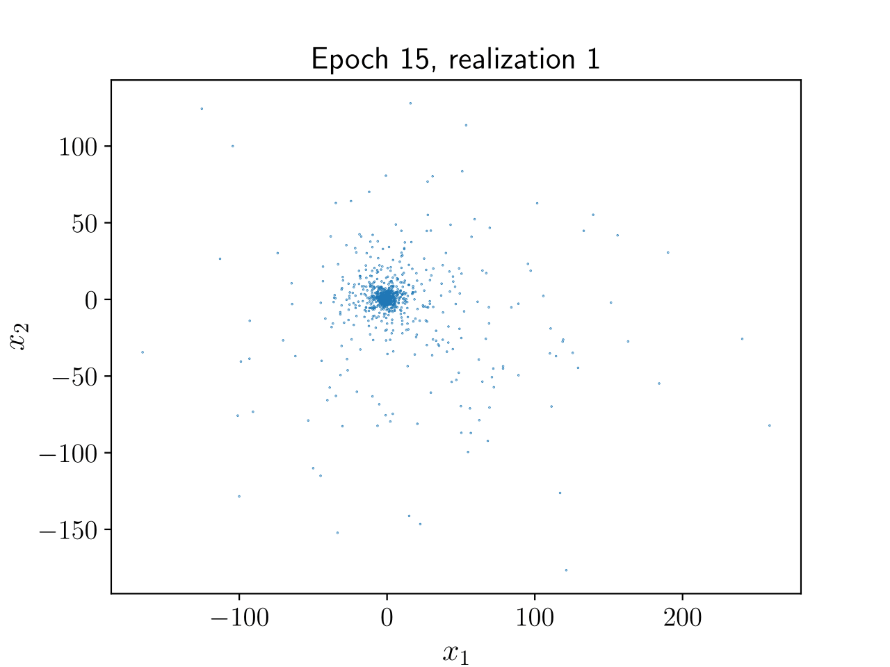
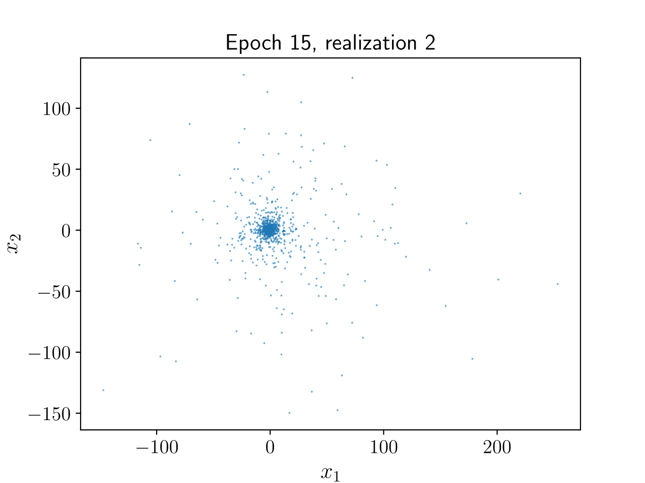
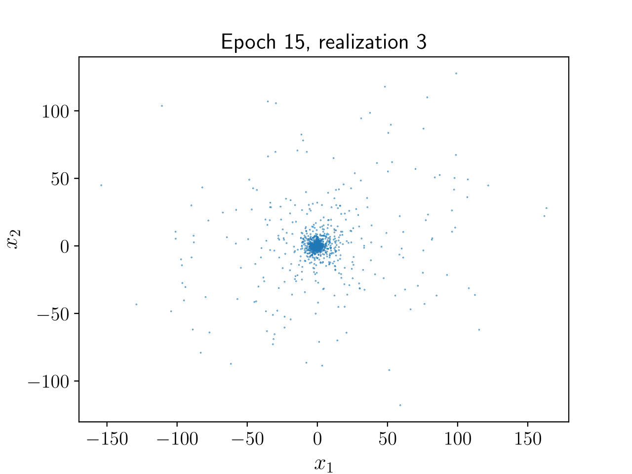
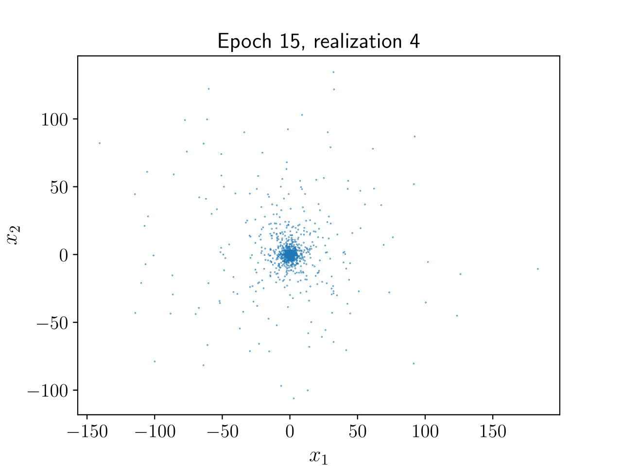
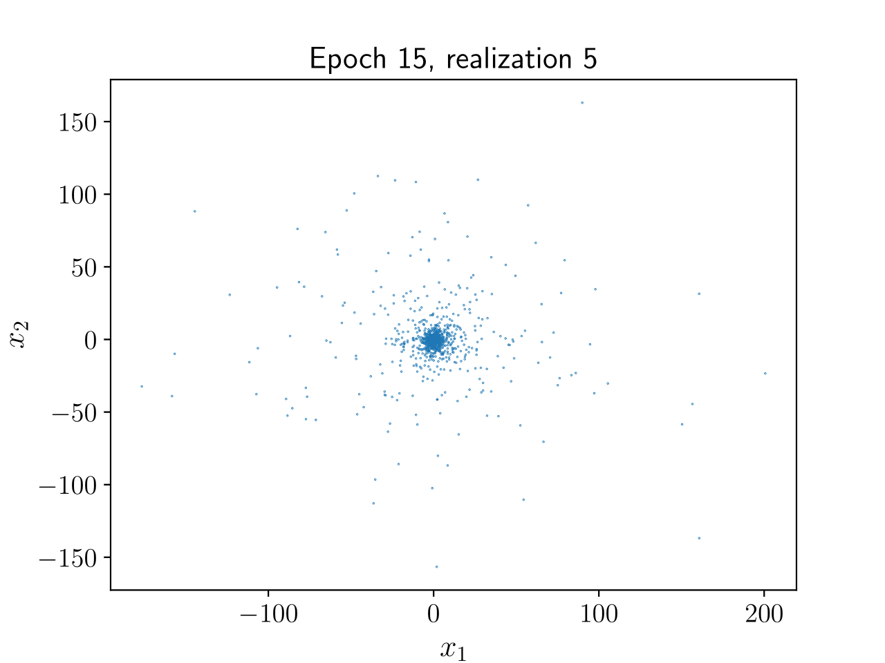
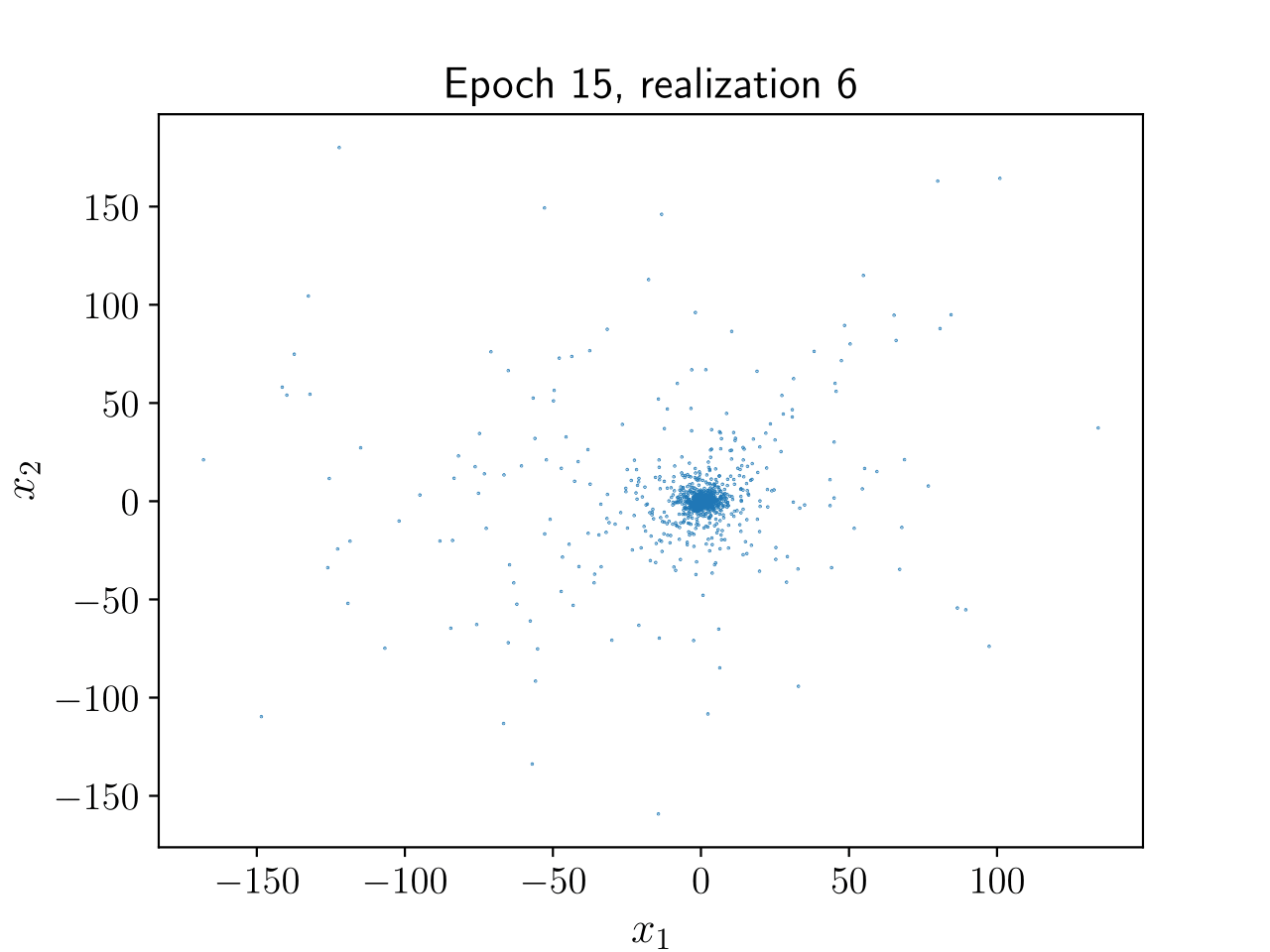
Figure 3: The distribution of gradient projections after training for 15 epochs, using 6 different projection matrices.

Nonlinearity Comparison - Additional Results.

Here, we present the results for the same setup as used in Section 4 in the main body, for a wider range of step-sizes and tail probability thresholds. Figure 4 provides the MSE behaviour of sign, joint and component-wise clipping for step-sizes $\alpha_{t}=\frac{1}{(t+1)^{\delta}}$, with $\delta\in\{17/24,3/4,7/8\}$, while Figure 5 presents the tail probability for all three methods, with step-size $\delta=3/4$ and using thresholds $\varepsilon\in\{0.05,0.1,0.5,5\}$ . We can see that the results from Section 4 are consistent for different ranges of step-sizes, confirming that joint clipping is not always the optimal choice of nonlinearity. Moreover, we can see that all three methods achieve exponential tail decay, with joint clipping requiring a larger threshold, as it converges slower than the other two nonlinear methods, reaching a lower accuracy in the allocated number of iterations.

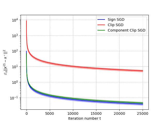
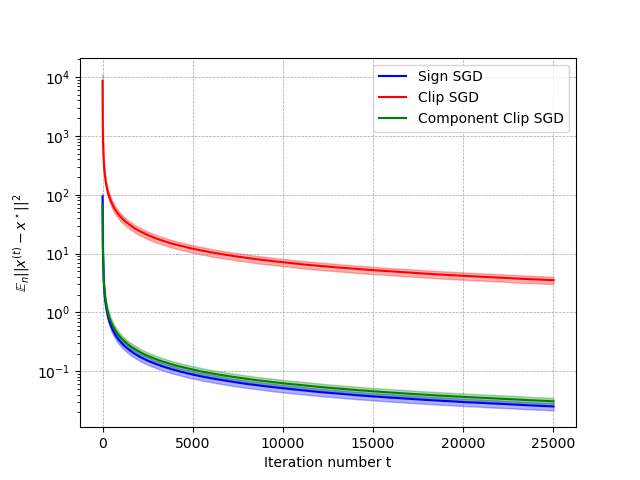
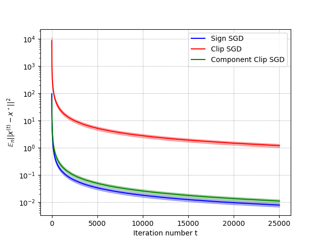
Figure 4: MSE performance of nonlinear SGD methods, using step-size policy $\alpha_{t}=1/(t+1)^{\delta}$, for different values of $\delta\in(2/3,1)$. Left to right: we choose the values $\delta\in\{17/24,3/4,7/8\}$, respectively. We can see that both component-wise nonlinearities converge faster in the MSE sense, independent of the step-size choice.

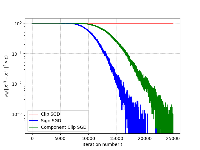
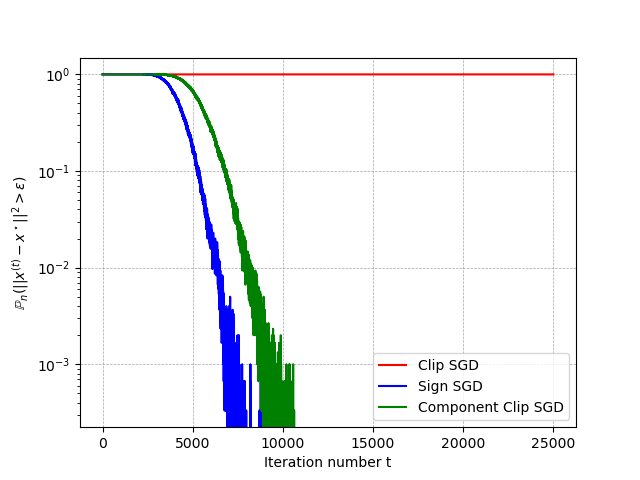
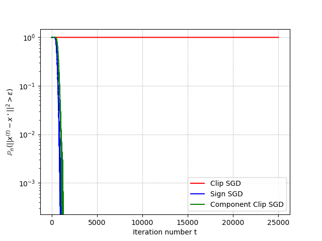
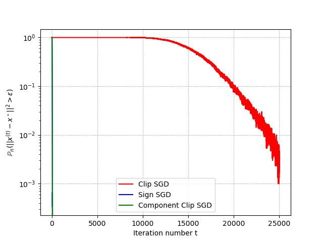
Figure 5: High-probability performance of nonlinear SGD methods, using step-size policy $\alpha_{t}=1/(t+1)^{\delta}$, with $\delta=3/4$. We use the thresholds $\varepsilon\in\{0.05,0.1,0.5,5\}$ to compute the tail probability, left to right and top to bottom. We can see that all the methods exhibit exponential tail decay, with joint clipping needing the largest threshold to achieve exponential decay, due to slower convergence.

Bibliography

- Alistarh et al., (2017) Alistarh, D., Grubic, D., Li, J., Tomioka, R., and Vojnovic, M. (2017). Qsgd: Communication-efficient sgd via gradient quantization and encoding. Advances in neural information processing systems, 30.
- Barsbey et al., (2021) Barsbey, M., Sefidgaran, M., Erdogdu, M. A., Richard, G., and Simsekli, U. (2021). Heavy tails in sgd and compressibility of overparametrized neural networks. In Ranzato, M., Beygelzimer, A., Dauphin, Y., Liang, P., and Vaughan, J. W., editors, Advances in Neural Information Processing Systems, volume 34, pages 29364–29378. Curran Associates, Inc.
- Battash et al., (2024) Battash, B., Wolf, L., and Lindenbaum, O. (2024). Revisiting the noise model of stochastic gradient descent. In Dasgupta, S., Mandt, S., and Li, Y., editors, Proceedings of The 27th International Conference on Artificial Intelligence and Statistics, volume 238 of Proceedings of Machine Learning Research, pages 4780–4788. PMLR.
- Bercovici et al., (1999) Bercovici, H., Pata, V., and Biane, P. (1999). Stable laws and domains of attraction in free probability theory. Annals of Mathematics, 149(3):1023–1060.
- (5) Bernstein, J., Wang, Y.-X., Azizzadenesheli, K., and Anandkumar, A. (2018a). signsgd: Compressed optimisation for non-convex problems. In International Conference on Machine Learning, pages 560–569. PMLR.
- (6) Bernstein, J., Zhao, J., Azizzadenesheli, K., and Anandkumar, A. (2018b). signsgd with majority vote is communication efficient and fault tolerant. arXiv preprint arXiv:1810.05291.
- Bottou, (2010) Bottou, L. (2010). Large-scale machine learning with stochastic gradient descent. In Proceedings of COMPSTAT’2010: 19th International Conference on Computational StatisticsParis France, August 22-27, 2010 Keynote, Invited and Contributed Papers, pages 177–186. Springer.
- Bottou et al., (2018) Bottou, L., Curtis, F. E., and Nocedal, J. (2018). Optimization methods for large-scale machine learning. SIAM Review, 60(2):223–311.
- Chen et al., (2020) Chen, X., Wu, S. Z., and Hong, M. (2020). Understanding gradient clipping in private sgd: A geometric perspective. Advances in Neural Information Processing Systems, 33:13773–13782.
- Crawshaw et al., (2022) Crawshaw, M., Liu, M., Orabona, F., Zhang, W., and Zhuang, Z. (2022). Robustness to unbounded smoothness of generalized signsgd. Advances in Neural Information Processing Systems, 35:9955–9968.
- Cutkosky and Mehta, (2020) Cutkosky, A. and Mehta, H. (2020). Momentum improves normalized sgd. In International conference on machine learning, pages 2260–2268. PMLR.
- Das et al., (2021) Das, R., Hashemi, A., Sanghavi, S., and Dhillon, I. S. (2021). Dp-normfedavg: Normalizing client updates for privacy-preserving federated learning. arXiv preprint arXiv:2106.07094.
- Davis et al., (2021) Davis, D., Drusvyatskiy, D., Xiao, L., and Zhang, J. (2021). From low probability to high confidence in stochastic convex optimization. The Journal of Machine Learning Research, 22(1):2237–2274.
- Eldowa and Paudice, (2023) Eldowa, K. and Paudice, A. (2023). General tail bounds for non-smooth stochastic mirror descent. arXiv preprint arXiv:2312.07142.
- Gandikota et al., (2021) Gandikota, V., Kane, D., Maity, R. K., and Mazumdar, A. (2021). vqsgd: Vector quantized stochastic gradient descent. In International Conference on Artificial Intelligence and Statistics, pages 2197–2205. PMLR.
- Ghadimi and Lan, (2012) Ghadimi, S. and Lan, G. (2012). Optimal stochastic approximation algorithms for strongly convex stochastic composite optimization i: A generic algorithmic framework. SIAM Journal on Optimization, 22(4):1469–1492.
- Ghadimi and Lan, (2013) Ghadimi, S. and Lan, G. (2013). Stochastic first-and zeroth-order methods for nonconvex stochastic programming. SIAM Journal on Optimization, 23(4):2341–2368.
- Gorbunov et al., (2020) Gorbunov, E., Danilova, M., and Gasnikov, A. (2020). Stochastic optimization with heavy-tailed noise via accelerated gradient clipping. Advances in Neural Information Processing Systems, 33:15042–15053.
- Gorbunov et al., (2021) Gorbunov, E., Danilova, M., Shibaev, I., Dvurechensky, P., and Gasnikov, A. (2021). Near-optimal high probability complexity bounds for non-smooth stochastic optimization with heavy-tailed noise. arXiv preprint arXiv:2106.05958.
- Gurbuzbalaban et al., (2021) Gurbuzbalaban, M., Simsekli, U., and Zhu, L. (2021). The heavy-tail phenomenon in sgd. In Meila, M. and Zhang, T., editors, Proceedings of the 38th International Conference on Machine Learning, volume 139 of Proceedings of Machine Learning Research, pages 3964–3975. PMLR.
- Hardt et al., (2016) Hardt, M., Recht, B., and Singer, Y. (2016). Train faster, generalize better: Stability of stochastic gradient descent. In International conference on machine learning, pages 1225–1234. PMLR.
- Harvey et al., (2019) Harvey, N. J., Liaw, C., Plan, Y., and Randhawa, S. (2019). Tight analyses for non-smooth stochastic gradient descent. In Conference on Learning Theory, pages 1579–1613. PMLR.
- Hazan and Kale, (2014) Hazan, E. and Kale, S. (2014). Beyond the regret minimization barrier: optimal algorithms for stochastic strongly-convex optimization. The Journal of Machine Learning Research, 15(1):2489–2512.
- Hazan et al., (2015) Hazan, E., Levy, K., and Shalev-Shwartz, S. (2015). Beyond convexity: Stochastic quasi-convex optimization. Advances in neural information processing systems, 28.
- Huber, (1964) Huber, P. J. (1964). Robust Estimation of a Location Parameter. The Annals of Mathematical Statistics, 35(1):73 – 101.
- Jakovetić et al., (2023) Jakovetić, D., Bajović, D., Sahu, A. K., Kar, S., Milošević, N., and Stamenković, D. (2023). Nonlinear gradient mappings and stochastic optimization: A general framework with applications to heavy-tail noise. SIAM Journal on Optimization, 33(2):394–423.
- Lan, (2012) Lan, G. (2012). An optimal method for stochastic composite optimization. Mathematical Programming, 133(1-2):365–397.
- LeCun et al., (2015) LeCun, Y., Bengio, Y., and Hinton, G. (2015). Deep learning. nature, 521(7553):436–444.
- LeCun et al., (1998) LeCun, Y., Cortes, C., and Burges, C. J. (1998). The mnist database of handwritten digits. http://yann. lecun. com/exdb/mnist/.
- Li and Liu, (2022) Li, S. and Liu, Y. (2022). High probability guarantees for nonconvex stochastic gradient descent with heavy tails. In International Conference on Machine Learning, pages 12931–12963. PMLR.
- Li and Orabona, (2020) Li, X. and Orabona, F. (2020). A high probability analysis of adaptive sgd with momentum. arXiv preprint arXiv:2007.14294.
- (32) Liu, Z., Nguyen, T. D., Nguyen, T. H., Ene, A., and Nguyen, H. (2023a). High probability convergence of stochastic gradient methods. In International Conference on Machine Learning, pages 21884–21914. PMLR.
- (33) Liu, Z., Zhang, J., and Zhou, Z. (2023b). Breaking the lower bound with (little) structure: Acceleration in non-convex stochastic optimization with heavy-tailed noise. In Neu, G. and Rosasco, L., editors, Proceedings of Thirty Sixth Conference on Learning Theory, volume 195 of Proceedings of Machine Learning Research, pages 2266–2290. PMLR.
- Madden et al., (2024) Madden, L., Dall’Anese, E., and Becker, S. (2024). High probability convergence bounds for non-convex stochastic gradient descent with sub-weibull noise. Journal of Machine Learning Research, 25(241):1–36.
- Moulines and Bach, (2011) Moulines, E. and Bach, F. (2011). Non-asymptotic analysis of stochastic approximation algorithms for machine learning. In Shawe-Taylor, J., Zemel, R., Bartlett, P., Pereira, F., and Weinberger, K., editors, Advances in Neural Information Processing Systems, volume 24. Curran Associates, Inc.
- Nair et al., (2022) Nair, J., Wierman, A., and Zwart, B. (2022). The Fundamentals of Heavy Tails: Properties, Emergence, and Estimation. Cambridge Series in Statistical and Probabilistic Mathematics. Cambridge University Press.
- Nemirovski et al., (2009) Nemirovski, A., Juditsky, A., Lan, G., and Shapiro, A. (2009). Robust stochastic approximation approach to stochastic programming. SIAM Journal on optimization, 19(4):1574–1609.
- Nesterov, (2018) Nesterov, Y. (2018). Lectures on Convex Optimization. Springer Publishing Company, Incorporated, 2nd edition.
- (39) Nguyen, T. D., Nguyen, T. H., Ene, A., and Nguyen, H. (2023a). Improved convergence in high probability of clipped gradient methods with heavy tailed noise. In Oh, A., Neumann, T., Globerson, A., Saenko, K., Hardt, M., and Levine, S., editors, Advances in Neural Information Processing Systems, volume 36, pages 24191–24222. Curran Associates, Inc.
- (40) Nguyen, T. D., Nguyen, T. H., Ene, A., and Nguyen, H. L. (2023b). High probability convergence of clipped-sgd under heavy-tailed noise. arXiv preprint arXiv:2302.05437.
- Parletta et al., (2022) Parletta, D. A., Paudice, A., Pontil, M., and Salzo, S. (2022). High probability bounds for stochastic subgradient schemes with heavy tailed noise. arXiv preprint arXiv:2208.08567.
- Peluchetti et al., (2020) Peluchetti, S., Favaro, S., and Fortini, S. (2020). Stable behaviour of infinitely wide deep neural networks. In Chiappa, S. and Calandra, R., editors, Proceedings of the Twenty Third International Conference on Artificial Intelligence and Statistics, volume 108 of Proceedings of Machine Learning Research, pages 1137–1146. PMLR.
- Polyak, (1990) Polyak, B. (1990). New stochastic approximation type procedures. Avtomatica i Telemekhanika, 7:98–107.
- Polyak and Juditsky, (1992) Polyak, B. and Juditsky, A. (1992). Acceleration of Stochastic Approximation by Averaging. SIAM Journal on Control and Optimization, 30:838–855.
- Polyak and Tsypkin, (1979) Polyak, B. and Tsypkin, Y. (1979). Adaptive estimation algorithms: Convergence, optimality, stability. Automation and Remote Control, 1979.
- Puchkin et al., (2023) Puchkin, N., Gorbunov, E., Kutuzov, N., and Gasnikov, A. (2023). Breaking the heavy-tailed noise barrier in stochastic optimization problems. arXiv preprint arXiv:2311.04161.
- Rakhlin et al., (2012) Rakhlin, A., Shamir, O., and Sridharan, K. (2012). Making gradient descent optimal for strongly convex stochastic optimization. In Proceedings of the 29th International Coference on International Conference on Machine Learning, pages 1571–1578.
- Robbins and Monro, (1951) Robbins, H. and Monro, S. (1951). A stochastic approximation method. The annals of mathematical statistics, pages 400–407.
- Ruppert, (1988) Ruppert, D. (1988). Efficient Estimations from a Slowly Convergent Robbins-Monro Process. Technical Report 781, Cornell University Operations Research and Industrial Engineering.
- Sadiev et al., (2023) Sadiev, A., Danilova, M., Gorbunov, E., Horváth, S., Gidel, G., Dvurechensky, P., Gasnikov, A., and Richtárik, P. (2023). High-probability bounds for stochastic optimization and variational inequalities: the case of unbounded variance. In International Conference on Machine Learning, pages 29563–29648. PMLR.
- (51) Simsekli, U., Gurbuzbalaban, M., Nguyen, T. H., Richard, G., and Sagun, L. (2019a). On the heavy-tailed theory of stochastic gradient descent for deep neural networks. arXiv preprint arXiv:1912.00018.
- (52) Simsekli, U., Sagun, L., and Gurbuzbalaban, M. (2019b). A tail-index analysis of stochastic gradient noise in deep neural networks. In International Conference on Machine Learning, pages 5827–5837. PMLR.
- Tsai et al., (2022) Tsai, C.-P., Prasad, A., Balakrishnan, S., and Ravikumar, P. (2022). Heavy-tailed streaming statistical estimation. In Camps-Valls, G., Ruiz, F. J. R., and Valera, I., editors, Proceedings of The 25th International Conference on Artificial Intelligence and Statistics, volume 151 of Proceedings of Machine Learning Research, pages 1251–1282. PMLR.
- Wright and Recht, (2022) Wright, S. J. and Recht, B. (2022). Optimization for Data Analysis. Cambridge University Press.
- Yang et al., (2022) Yang, X., Zhang, H., Chen, W., and Liu, T.-Y. (2022). Normalized/clipped sgd with perturbation for differentially private non-convex optimization. arXiv preprint arXiv:2206.13033.
- You et al., (2019) You, Y., Li, J., Hseu, J., Song, X., Demmel, J., and Hsieh, C.-J. (2019). Reducing bert pre-training time from 3 days to 76 minutes. arXiv preprint arXiv:1904.00962, 12.
- Yu and Kar, (2023) Yu, S. and Kar, S. (2023). Secure distributed optimization under gradient attacks. IEEE Transactions on Signal Processing, 71:1802–1816.
- Zeiler, (2012) Zeiler, M. D. (2012). Adadelta: an adaptive learning rate method. arXiv preprint arXiv:1212.5701.
- Zhang et al., (2019) Zhang, J., He, T., Sra, S., and Jadbabaie, A. (2019). Why gradient clipping accelerates training: A theoretical justification for adaptivity. In International Conference on Learning Representations.
- Zhang et al., (2020) Zhang, J., Karimireddy, S. P., Veit, A., Kim, S., Reddi, S., Kumar, S., and Sra, S. (2020). Why are adaptive methods good for attention models? Advances in Neural Information Processing Systems, 33:15383–15393.
- Zhang et al., (2022) Zhang, X., Chen, X., Hong, M., Wu, Z. S., and Yi, J. (2022). Understanding clipping for federated learning: Convergence and client-level differential privacy. In International Conference on Machine Learning, ICML 2022.