Triple gauge coupling analysis using boosted $W$’s and $Z$’s

Abstract

We analyze the Large Hadron Collider potential to study triple couplings of the electroweak gauge bosons using their boosted hadronic decays. Deviations from Standard Model predictions spoil cancelations present in the Standard Model leading to the growth of the electroweak diboson production cross section at high center-of-mass energies. In this kinematical limit, $W$’s and $Z$’s are highly boosted, and consequently, their hadronic decays give rise to fat jets. Here, we show that the study of boosted hadronically decaying $W$ and $Z$ leads to limits on triple gauge couplings that are comparable to the ones originating from the leptonic decay channels.

I Introduction

The CERN Large Hadron Collider (LHC) has already accumulated a substantial dataset allowing for precision tests of the Standard Model (SM) and searches for new physics. Within the SM framework, the triple and quartic vector-boson couplings are determined by the non-abelian $SU(2)_{L}\otimes U(1)_{Y}$ gauge symmetry, being completely fixed in terms of the gauge couplings. Possible deviations from the SM predictions for the triple gauge couplings (TGC) are a clear sign of new physics and consequently, TGCs are investigated at the LHC in charged processes like $W^{+}W^{-}$, $W^{\pm}Z$ and $W^{\pm}\gamma$ productions.

Anomalous TGC can be generated by integrating out new heavy states, however, the resulting anomalous couplings are suppressed by loop factors $1/(16\pi^{2})$ for weakly interacting extensions of the SM Arzt et al. (1995). Notwithstanding, it is possible to write down ultraviolet extensions of the SM that generate anomalous TGC at tree level and that are not constrained by the electroweak precision observables Falkowski et al. (2017); Arkani-Hamed et al. (2001).

Due to the importance of TGC measurements, the ATLAS and CMS collaborations conduct studies on the electroweak TGC through various processes. They analyze the $W^{\pm}Z\to\ell^{+}\ell^{-}\ell^{\prime\pm}+E_{T}^{\text{miss}}$ channel ATLAS Collaboration (2018); CMS Collaboration (2021a) as well as the $W^{+}W^{-}\to\ell^{+}\ell^{(\prime)-}+E_{T}^{\text{miss}}$ final state Sirunyan et al. (2020); Aad et al. (2021). Additionally, TGC were investigated in the $W^{\pm}\gamma\to\ell^{\pm}\gamma+E_{T}^{\text{miss}}$ production CMS Collaboration (2021b). The ATLAS collaboration further explored the semileptonic reaction $WW/WZ\to\ell\nu qq^{\prime}$ at 8 TeV Aaboud et al. (2017) to extract limits on anomalous TGCs, with the most stringent constraints arising from cases where a single fat jet was tagged as a $W$ or $Z$ boson.

In this work, we analyze the $WW/WZ$ and $W\gamma$ diboson productions in the fully hadronic final state, focusing on scenarios where the boosted $W/Z$ bosons are identified as high transverse momentum and large-radius jets. We utilize the large-radius jet mass and its substructure to effectively characterize the hadronically decaying $W/Z$ bosons and to reduce Standard Model backgrounds. To demonstrate the potential of these new channels for TGC studies, we recast the ATLAS searches for heavy resonances decaying into $WW/WZ$ in the hadronic channel Aad et al. (2019) as well as $W\gamma$ Aad et al. (2023). We show that these processes can lead to TGC bounds comparable to the ones obtained by studying leptonic final states. Moreover, we also analyze the potential of the High Luminosity LHC (HL-LHC) run to probe anomalous TGC in all-hadronic electroweak diboson (EWDB) channels, i.e. in the production of pairs $WZ$, $WW$ and $W\gamma$.

This work is organized as follows: in Section II we present the adopted theoretical framework as well as the analyses methodology. Section III contains our results and we summarize our conclusions in section IV.

II Analysis Framework

Assuming the existence of a mass gap between the new physics energy scale and the electroweak one, we parametrize the deviations from the SM TGC predictions using effective field theory. Furthermore, assuming that the scalar particle observed in 2012 Aad et al. (2012); Chatrchyan et al. (2012) belongs to an electroweak doublet, we can realize the $SU(2)_{L}\otimes U(1)_{Y}$ symmetry linearly, i.e. we work in the Standard Model Effective Field Theory (SMEFT) framework. We choose the Hagiwara, Ishihara, Szalapski, and Zeppenfeld (HISZ) dimension-six basis Hagiwara et al. (1993, 1997) and we consider three operators contributing to TGC at dimension-six:

$${\cal O}_{W}=(D_{\mu}\Phi)^{\dagger}\widehat{W}^{\mu\nu}(D_{\nu}\Phi)\;\;\;\;,\;\;\;\; {\cal O}_{B}=(D_{\mu}\Phi)^{\dagger}\widehat{B}^{\mu\nu}(D_{\nu}\Phi)\;\;\;\;,\;\;\;\; {\cal O}_{WWW}={\rm Tr}[\widehat{W}_{\mu}^{\nu}\widehat{W}_{\nu}^{\rho}\widehat{W}_{\rho}^{\mu}]\;,$$ (1)

where $\Phi$ stands for the SM Higgs doublet and we have defined $\widehat{B}_{\mu\nu}\equiv i(g^{\prime}/2)B_{\mu\nu}$ and $\widehat{W}_{\mu\nu}\equiv i(g/2)\sigma^{a}W^{a}_{\mu\nu}$, with $g$ and $g^{\prime}$ being the $SU(2)_{L}$ and $U(1)_{Y}$ gauge couplings, respectively. Here $\sigma^{a}$ represents the Pauli matrices. In this work we considered the dimension-six effective lagrangian,

$${\cal L}_{\rm eff}={\cal L}_{\rm SM}+\frac{f_{W}}{\Lambda^{2}}{\cal O}_{W}+\frac{f_{B}}{\Lambda^{2}}{\cal O}_{B}+\frac{f_{WWW}}{\Lambda^{2}}{\cal O}_{WWW}\;,$$ (2)

where $\Lambda$ is the characteristic mass scale of new physics and $f_{W,B,WWW}$ are the Wilson coefficients.

The above TGC operators can be qualitatively understood in terms of the effective $\gamma W^{+}W^{-}$ and $ZW^{+}W^{-}$ parametrization introduced in Ref. Hagiwara et al. (1987)

$${\cal L}_{WWV}=-ig_{WWV}\Big{\{}g_{1}^{V}\Big{(}W^{+}_{\mu\nu}W^{-\,\mu}V^{\nu}-W^{+}_{\mu}V_{\nu}W^{-\,\mu\nu}\Big{)}+\kappa_{V}W_{\mu}^{+}W_{\nu}^{-}V^{\mu\nu}+\frac{\lambda_{V}}{\widehat{M}_{W}^{2}}W^{+}_{\mu\nu}W^{-\,\nu\rho}V_{\rho}^{\;\mu}\Big{\}}\;\;,$$ (3)

where $V=\gamma,\,Z$, $g_{WW\gamma}=\hat{e}$, $g_{WWZ}=\hat{e}\hat{c}/\hat{s}$, and $\widehat{M}_{W}=\hat{e}\hat{v}/2\hat{s}$, with $\hat{e}$ representing the proton electric charge and $\hat{c}(\hat{s})$ denoting the sine (cosine) of the weak mixing angle. In the SM, $g_{1}^{\gamma}=g_{1}^{Z}=\kappa_{\gamma}=\kappa_{Z}=1$ and $\lambda_{Z}=\lambda_{\gamma}=0$. After including the direct contribution from the dimension-six operators, electromagnetic gauge invariance still enforces $g_{1}^{\gamma}=1$, while the other effective TGC couplings read:

$$\Delta g_{1}^{Z}=\frac{\hat{e}^{2}}{8\hat{s}^{2}\hat{c}^{2}}\frac{\hat{v}^{2}}{\Lambda^{2}}f_{W}\;,$$

$$\Delta\kappa_{\gamma}=\frac{\hat{e}^{2}}{8\hat{s}^{2}}\frac{\hat{v}^{2}}{\Lambda^{2}}\left(f_{W}+f_{B}\right)\;,$$

$$\Delta\kappa_{Z}=\frac{\hat{e}^{2}}{8\hat{s}^{2}}\frac{\hat{v}^{2}}{\Lambda^{2}}\left[f_{W}-\frac{\hat{s}^{2}}{\hat{c}^{2}}f_{B}\right]\;,$$ (4)

$$\lambda_{\gamma}=\lambda_{Z}=\frac{3\hat{e}^{2}}{2\hat{s}^{2}}\frac{\widehat{M}_{W}^{2}}{\Lambda^{2}}f_{WWW}\;.$$

In addition to the TGC contributions, diboson production can also be modified by anomalous couplings of the gauge bosons to fermions. However, electroweak precision data impose strong constraints on such couplings Butter et al. (2016); da Silva Almeida et al. (2019); Alves et al. (2018); Almeida et al. (2021); Corbett et al. (2023) and ergo we do not take these contributions into account.

We simulate the EWDB channels at leading order using MadGraph5_aMC@NLO Frederix et al. (2018) with the UFO files for our effective Lagrangian generated with FeynRules Christensen and Duhr (2009); Alloul et al. (2014). We employ PYTHIA8 Sjostrand et al. (2008) to perform the parton shower and hadronization, while the fast detector simulation is carried out with Delphes de Favereau et al. (2014). Jet analyses are performed using FASTJET Cacciari et al. (2012). For the EWDB hadronic channels, the final jets were clustered and trimmed in the same way as described by the experimental collaborations Aad et al. (2019, 2023), using the final state stable particles after performing the parton-shower and hadronization. The analysis of the jet-substructure was carried out using the plugins that are part of the FASTJET contrib project (https://fastjet.hepforge.org/contrib/).

	Channel ($a$)	Distribution	# bins	Data set	Int Lum
	$WZ\to\ell^{+}\ell^{-}\ell^{\prime\pm}$	$M(WZ)$	7	CMS 13 TeV,	137.2 fb-1 CMS Collaboration (2021a)
EWDB data	$WW\to\ell^{+}\ell^{(\prime)-}+0/1j$	$M(\ell^{+}\ell^{(\prime)-})$	11	CMS 13 TeV,	35.9 fb-1 Sirunyan et al. (2020)
	$W\gamma\to\ell\nu\gamma$	$\frac{d^{2}\sigma}{dp_{T}d\phi}$	12	CMS 13 TeV,	137.1 fb-1 CMS Collaboration (2021b)
	$WW\rightarrow e^{\pm}\mu^{\mp}+/\!\!\!E_{T}\;(0j)$	$m_{T}$	17 (15)	ATLAS 13 TeV,	36.1 fb-1 Aaboud et al. (2018)
	$WZ\rightarrow\ell^{+}\ell^{-}\ell^{(\prime)\pm}$	$m_{T}^{WZ}$	6	ATLAS 13 TeV,	36.1 fb-1 ATLAS Collaboration (2018)
	$WW\rightarrow\ell^{+}\ell^{(\prime)-}+/\!\!\!E_{T}\;(1j)$	$\frac{d\sigma}{dm_{\ell^{+}\ell^{-}}}$	10	ATLAS 13 TeV,	139 fb-1 Aad et al. (2021)
	$WW/WZ\rightarrow 2J$	$M_{JJ}$	11	ATLAS 13 TeV	139 fb-1 Aad et al. (2019)
	$W\gamma\rightarrow J\gamma$	$M(J\gamma)$	20	ATLAS 13 TeV	139 fb-1 Aad et al. (2023)

Table 1: EWDB data from LHC used in the analyses. For the $W^{+}W^{-}$ results from ATLAS run 2 Aaboud et al. (2018) we combine the data from the last three bins into one to ensure gaussianity.

In this work, we considered two scenarios in our analyses. In the first scenario, we used the available Run 2 experimental data, which contains an integrated luminosity of $139$ fb^-1. In the second scenario, we performed our analyses for the hadronic EWDB channels assuming the foreseen integrated luminosity of the High Luminosity LHC run, i.e. $3000$ fb^-1, however, we kept the present experimental systematic errors.

Table 1 presents the Run 2 EWDB data used in our analyses, comprising a total of $92$ data points. In order to improve the statistical analysis of the hadronic channels, we rebinned the data. For the $W\gamma\rightarrow J\gamma$ channel, we merged the bins of the distribution in such a way that the total number of events in each bin can be described by a Gaussian distribution. For the ATLAS $WW/WZ\rightarrow 2J$ channel, the bins were combined to ensure at least one event per bin. In summary, the binnings used in our Run 2 analyses are as follows:

$$\text{ATLAS }W\gamma\rightarrow J\gamma:\;\;$$

$$(0.80,0.88,0.96,1.04,1.12,1.20,1.28,1.36,1.44,1.52,$$

$$1.60,1.68,1.76,1.84,1.92,2.00,2.12,2.28,2.56,2.96,7.00)\;\hbox{ TeV}$$

$$\text{ATLAS }WW/WZ\rightarrow 2J:\;\;$$

$$(1.30,1.40,1.50,1.60,1.70,1.80,1.90,2.00,2.10,2.40,3.10,5.10)\;\hbox{ TeV}.$$

On the other hand, our choice of bins for the HL-LHC analyses is

$$\text{ATLAS }W\gamma\rightarrow J\gamma:\;\;$$

$$(0.80,0.92,1.00,1.08,1.16,1.24,1.36,1.48,1.60,1.72,1.84,1.96,$$

$$2.08,2.20,2.32,2.44,2.56,2.68,2.80,2.96,3.12,3.28,3.48,3.76,4.24,7.00)\;\hbox{ TeV}$$

$$\text{ATLAS }WW/WZ\rightarrow 2J:\;\;$$

$$(1.30,1.40,1.60,1.80,2.00,2.20,2.40,2.60,2.90,3.40,5.10)\;\hbox{ TeV}.$$

In Fig. 1, we exhibit the anomalous TGC and background invariant mass distributions for the all hadronic EWDB channels, using illustrative values of the relevant Wilson coefficients, along with the experimental data extracted from Aad et al. (2023, 2019) for the Run 2 analysis. Notice that ${\cal O}_{B}$ and ${\cal O}_{W}$ contribute in the same way to $W\gamma$ production; see Eq. (4). As we can see, the presence of anomalous TGC enhances the cross section at large invariant masses. This behavior is expected, as the additional TGC contributions spoil the SM high-energy cancellations.

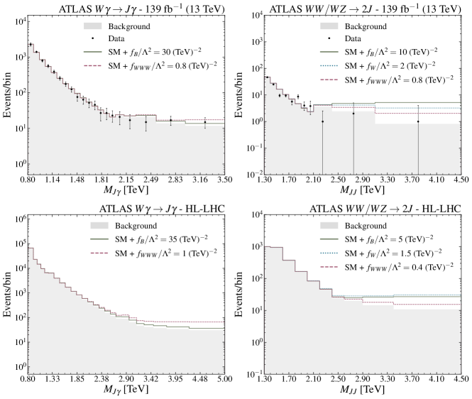
Figure 1: Kinematical distributions employed in the hadronic analyses. The left (right) pannels display the anomalous TGC and background $M_{J\gamma}$ ($M_{JJ}$) invariant mass distribution for illustrative values of the dimension-six Wilson coefficients. On the first row, we present the distributions used for the Run 2 analyses, while on the bottom the ones used for the HL-LHC analyses. We used the fit to the background performed in the experimental analyses Aad et al. (2019, 2023) for all of our studies, except that in the HL-LHC case, we rescaled it with the proper luminosity. On the left pannels, the last bin contains events up to 7 TeV, while on the right pannels, the last bin contains events up to 5.1 TeV.

We performed the statistical analysis of the leptonic EWDB data using the binned chi-squared function described in Ref. Corbett et al. (2023). On the other hand, for the analysis of the ATLAS $W\gamma\rightarrow J\gamma$ channel, we profited from the gaussianity of the combined bins and defined the chi-square function

$$\chi^{2}(f_{B},f_{W},f_{WWW})=\min_{\vec{\xi}}\Bigg{\{}\sum_{i}\Bigg{(}\dfrac{N_{i}^{\text{obs}}-N_{i}^{\text{th}}}{\sigma_{i}}\Bigg{)}^{2}+\xi_{1}^{2}+\xi_{2}^{2}\Bigg{\}},$$ (5)

where $N_{i}^{\text{obs}}$ represents the observed number of events in the bin $i$ while the theory prediction is given by

$$N_{i}^{\text{th}}=\big{(}1+\sigma_{\xi_{1}}\xi_{1}\big{)}N^{\text{signal}}_{i}+\big{(}1+\sigma_{\xi_{2}}\xi_{2}\big{)}N_{i}^{\text{backg}} N^{\text{signal}}_{i}=N^{\text{int}}_{i}+N^{\text{BSM}}_{i},$$ with (6)

where $N^{\text{backg}}_{i}$ denotes the number of background events extracted from Ref. Aad et al. (2023), $N^{\text{int}}_{i}$ stands for the expected number of events originating from the interference between the dimension-six operator and SM contributions, and $N^{\text{BSM}}_{i}$ is the pure anomalous contribution to the number of expected events. Moreover, the $\sigma_{i}$ contains the statistical and background uncertainties added in quadrature, given by $\sigma_{i}^{2}=N^{\text{obs}}_{i}+\sigma_{\text{backg},i}^{2}$ where the last term in this expression was extracted from Ref. Aad et al. (2023). In order to account for possible systematic theoretical and experimental uncertainties, we defined two pulls Fogli et al. (2002), $\xi_{1}$ and $\xi_{2}$, affecting the normalization of the signal and background, respectively. The values chosen for $\sigma_{\xi_{1}}$ and $\sigma_{\xi_{2}}$ are 0.2 and 0.3, respectively. The values for $\sigma_{\xi_{1}}$ and $\sigma_{\xi_{2}}$ were estimated analysing the systematic errors from Ref. Aad et al. (2023). Although it is not possible to extract precise uncertainties from the available data, we made conservative estimates. Moreover, we expect the uncertainties on the signal to be slightly smaller than those on the background. In this case, an analytical expression for the pulls can be found by minimizing Eq. (5) with respect to $\xi_{1}$ and $\xi_{2}$.

The statistical analyses of the ATLAS $WW/WZ\rightarrow 2J$ channel were based on the chi-square function Fogli et al. (2002)

$$\chi^{2}(f_{B},f_{W},f_{WWW})=\min_{\vec{\xi}}\Bigg{\{}2\sum_{i}\Big{[}N_{i}^{\text{th}}-N_{i}^{\text{obs}}+N_{i}^{\text{obs}}\log\Big{(}\dfrac{N_{i}^{\text{obs}}}{N_{i}^{\text{th}}}\Big{)}\Big{]}+\xi_{1}^{2}+\xi_{2}^{2}\Bigg{\}},$$ (7)

with $N_{i}^{\text{obs}}$ standing for the observed number of events in the $i^{\text{th}}$ bin and $N_{i}^{\text{th}}$ defined as

$$N_{i}^{\text{th}}=\big{(}1+\sigma^{\xi_{1}}_{i}\xi_{1}\big{)}N^{\text{signal}}_{i}+\big{(}1+\sigma^{\xi_{2}}_{i}\xi_{2}\big{)}N_{i}^{\text{backg}} N^{\text{signal}}_{i}=N^{\text{int}}_{i}+N^{\text{BSM}}_{i},$$ with (8)

where $N_{i}^{\text{backg}}$, $N_{i}^{\text{int}}$ and $N_{i}^{\text{BSM}}$ represent the background-fit extracted from Ref. Aad et al. (2019), and the linear and quadratic contributions of the dimension-six operators, respectively. The systematic uncertainties were parameterized by the nuisance parameters $\xi_{1}$ and $\xi_{2}$, which modify the normalization of the signal and background, respectively. We chose the values for $\sigma^{\xi_{2}}_{i}$ to best represent the experimental errors, and for $\sigma^{\xi_{1}}_{i}$, the values chosen stem from the theoretical uncertainties. Their values are

$$\sigma_{i}^{\xi_{1}} =(0.05,0.05,0.05,0.05,0.1,0.1,0.1,0.15,0.15,0.15,0.15)\;,$$ (9)

$$\sigma_{i}^{\xi_{2}} =(0.1,0.1,0.2,0.2,0.4,0.4,0.5,0.5,1.0,1.0,1.0)\;.$$ (10)

The HL-LHC analysis is carried out to estimate how the limits on the Wilson coefficients $f_{B}$, $f_{W}$ and $f_{WWW}$, extracted using the hadronic EWDB channels, can improve with the upcoming LHC runs. Since there is no available data, we use the SM background fit scaled by a factor of 3000/139 as the observed number of events. As shown in the bottom row of Fig. 1, the number of events for each bin of the distributions for the $W\gamma$ and $WW/WZ$ channels is sufficiently large, allowing us to assume gaussianity. To extract the 95% CL intervals, we use the same statistics defined in Eq. (5), with minor modifications to the uncertainties. For the ATLAS $W\gamma\rightarrow J\gamma$, we rescaled the $\sigma_{\text{backg},i}$ to maintain the current $\sigma_{\text{backg},i}/N_{i}^{\text{obs}}$ ratio. For the ATLAS $WW/WZ\rightarrow 2J$, we defined $\sigma_{\text{backg},i}=x_{i}N^{\text{backg}}_{i}$, with

$$x_{i}=(0.1,0.1,0.2,0.2,0.4,0.4,0.5,0.5,1.0,1.0),$$ (11)

to represent the same large uncertainties in the background as the current data.

III Results

To estimate the LHC potential for studying TGC using highly boosted $W$’s and $Z$’s decaying hadronically, we recast the available ATLAS data on searches for resonances decaying into $WW/WZ$ and $W\gamma$ pairs followed by the hadronic decays of the gauge bosons Aad et al. (2019, 2023). For comparison, we also obtained the Run 2 limits from combining fully leptonic modes; for details see Ref. Corbett et al. (2023).

Table 2 presents the 95% CL allowed intervals for the three TGC Wilson coefficients contributing to diboson production. In the second and third columns, we exhibit the results for the analysis performed using the hadronic $WW/WZ$ production data and the hadronic $W\gamma$ results, respectively. For the sake of comparison, the fourth and fifth columns contain the allowed intervals using the leptonic final states of the $WW/WZ$ and $W\gamma$ diboson productions. Taking into account only the fully hadronic final states, the Wilson coefficients $f_{B}$ and $f_{W}$ are better constrained by the $WW/WZ$ diboson production. Additionally, $f_{WWW}$ is more tightly constrained than $f_{W}$ and $f_{B}$, with the $W\gamma$ production channel leading to the strongest bound. Comparing these results with those obtained from the leptonic decay modes, we can see that the fully hadronic channels lead to tighter limits on $f_{B}$, due to the $2J$ final state, while a similar limit is obtained for $f_{W}$. Moreover, the constraints for $f_{WWW}$ are similar for all channels.

Coefficient	Hadronic EWDB $(\mathcal{L}=139\rm\,fb^{-1})$		Leptonic EWDB $(\mathcal{L}=139\rm\,fb^{-1})$
	ATLAS $WW/WZ\rightarrow 2J$	ATLAS $W\gamma\rightarrow J\gamma$	Combined $WW/WZ$	CMS $W\gamma\rightarrow\ell\nu\gamma$
$\dfrac{f_{B}}{\Lambda^{2}}$	[-8.4, 8.8]	[-33, 33]	[-13, 15]	[-17, 19]
$\dfrac{f_{W}}{\Lambda^{2}}$	[-2.0, 2.3]	[-33, 33]	[-1.3, 2.5]	[-17, 19]
$\dfrac{f_{WWW}}{\Lambda^{2}}$	[-1.3, 1.3]	[-0.82, 0.82]	[-1.6, 1.6]	[-0.84, 0.74]

Table 2: 95% CL intervals for the TGC Wilson coefficients originating from the different datasets. We marginalized the chi-square with respect the other parameters in the analysis with the only exception being the $W\gamma$ channels for which we only included $f_{B}$ since its contribution is identical to the $f_{W}$ one, leading to a blind direction. In the fourth column we combined all the available data on $WW$ and $WZ$ production with the gauge bosons decaying to leptons.

To compare the impact of the different datasets on the study of anomalous TGC, Figure 2 depicts the $1\sigma$ and $2\sigma$ allowed regions for all parameters in the analyses as well as the one-dimensional projection of the $\Delta\chi^{2}$. As we can see, the hadronic datasets lead to more stringent constraints on $f_{B}$ than the leptonic ones, while the bounds on $f_{W}$ are comparable for the hadronic and leptonic final states; see Table 3 for the marginalized 95% CL allowed intervals. For all the hadronic (leptonic) results quoted in Table 3, we combine all the hadronic (leptonic) channels mentioned in Table 2. Notably, combining the $WW/WZ$ and $W\gamma$ hadronic datasets breaks the blind direction $f_{W}+f_{B}$ that exists in the $W\gamma$ production. As could have been anticipated, the combination of the hadronic channels gives bounds on $f_{WWW}$ similar to the ones originating from the leptonic final states; see Table 3. The combination of leptonic and hadronic channels leads, obviously, to more stringent limits.

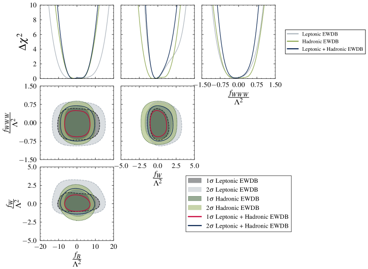
Figure 2: $1\sigma$ and $2\sigma$ allowed regions for each possible pair of Wilson coefficients in the analysis, after marginalizing over the undisplayed parameters, for the different datasets as indicated in the figure. We also display the one-dimensional marginalized projections of the $\Delta\chi^{2}$.

Coefficients	Hadronic EWDB $(\mathcal{L}=139\rm\,fb^{-1})$	Leptonic EWDB $(\mathcal{L}=139\rm\,fb^{-1})$	Leptonic $+$ Hadronic EWDB $(\mathcal{L}=139\rm\,fb^{-1})$
$\dfrac{f_{B}}{\Lambda^{2}}$	[-8.3, 8.7]	[-12, 12]	[-7.8, 8.4]
$\dfrac{f_{W}}{\Lambda^{2}}$	[-2.0, 2.3]	[-1.3, 2.6]	[-1.2, 1.7]
$\dfrac{f_{WWW}}{\Lambda^{2}}$	[-0.78, 0.78]	[-0.83, 0.72]	[-0.66, 0.60]

Table 3: 95% CL intervals for the TGC Wilson coefficients in the analysis of the hadronic channels, the result taking into account all leptonic channels, as well as the combination of leptonic and hadronic channels. In the hadronic (leptonic) results of this table we combine all the hadronic (leptonic) channels mentioned in Table 2.

We also obtained the attainable limits on the hadronic channel for the HL-LHC. We assumed that the observed number of events is the one predict by the fit to the SM background made by the ATLAS collaboration Aad et al. (2019, 2023). We also kept the same systematic uncertainties of this fit for the LHC Run 2 and we considered an integrated luminosity of 3000 fb^-1. Our results are presented in Table 4. As we can see, the HL-LHC can improve the present limits on the $f_{B}$ and $f_{WWW}$ coefficients (see last column of Table 3) by almost a factor of 1.5 when we consider only the hadronic channels in contrast with the current Leptonic limits.

Coefficient	Hadronic EWDB ($\mathcal{L}=3000\rm\,fb^{-1})$
	ATLAS $WW/WZ$	ATLAS $W\gamma$	Combined $WW/WZ$ and $W\gamma$
$\dfrac{f_{B}}{\Lambda^{2}}$	[-5.3, 5.6]	[-20, 20]	[-5.3, 5.6]
$\dfrac{f_{W}}{\Lambda^{2}}$	[-1.2, 1.5]	[-20, 20]	[-1.2, 1.5]
$\dfrac{f_{WWW}}{\Lambda^{2}}$	[-0.81, 0.81]	[-0.40, 0.40]	[–0.40, 0.40]

Table 4: 95% CL allowed intervals for the TGC Wilson coefficients for the hadronic model $WW/WZ$ and $W\gamma$ as well as their combination. We assumed an integrated luminosity of 3000 fb^-1.

IV Final remarks

We analyzed the LHC potential to probe anomalous TGC using the $WW/WZ$ and $W\gamma$ channels when the $W$’s and $Z$’s decay hadronically. We considered boosted final states where the $W/Z$ decay products give rise to a fat jet. In our analyses, we performed the same sequence of cuts used by the ATLAS collaboration for the search of heavy resonances Aad et al. (2019, 2023). We also considered the SM background as evaluated in the experimental studies.

To gauge our results, we compared the limits of the TGC Wilson coefficients derived from the fully hadronic mode with the ones from the leptonic final state. Our results indicate that the limits from leptonic and hadronic channels are similar. Ergo, the addition of the hadronic mode to the TGC analysis will lead to more stringent global fits.

Finally, we should conclude by reiterating the fact that the results presented in this paper relies heavily on the experimental fit to the SM background and the fits have large systematic uncertainties. In fact, this even leaves a room for improvement if the systematic uncertainties can be reduced for the high luminosity run of the LHC.