Optimal Transport for Probabilistic Circuits

Abstract

We introduce a novel optimal transport framework for probabilistic circuits (PCs). While it has been shown recently that divergences between distributions represented as certain classes of PCs can be computed tractably, to the best of our knowledge, there is no existing approach to compute the Wasserstein distance between probability distributions given by PCs. We consider a Wasserstein-type distance that restricts the coupling measure of the associated optimal transport problem to be a probabilistic circuit. We then develop an algorithm for computing this distance by solving a series of small linear programs and derive the circuit conditions under which this is tractable. Furthermore, we show that we can also retrieve the optimal transport plan between the PCs from the solutions to these linear programming problems. We then consider the empirical Wasserstein distance between a PC and a dataset, and show that we can estimate the PC parameters to minimize this distance through an efficient iterative algorithm.

1 Introduction

Modeling probability distributions in a way that enables tractable computation of certain probabilistic queries is of great interest to the machine learning community. Probabilistic circuits (PCs) [3] provide a unifying framework for representing many classes of tractable probabilistic models as computational graphs. They have received attention lately for the ability to guarantee tractable inference of certain query classes through imposing structural properties on the computational graph of the circuit. This includes tractable marginal and conditional inference, as well as pairwise queries that compare two circuits such as Kullback-Leibler Divergence and cross-entropy [9, 17].

However, to the best of our knowledge, there is no existing algorithm to compute the Wasserstein distance between two probabilistic circuits.

Definition 1 (Wasserstein distance)

Let $P$ and $Q$ be two probability measures on a metric space. For $p\geq 1$, the $p$-Wasserstein distance between $P$ and $Q$ is $\textsf{W}_{p}^{p}(P,Q)\triangleq\inf_{\gamma\in\Gamma(P,Q)}\operatorname{\mathbb{E}}_{\gamma(\mathbf{x},\mathbf{y})}[\left\lVert\mathbf{x}-\mathbf{y}\right\rVert_{p}^{p}]$ where $\Gamma(P,Q)$ denotes the set of all couplings which are joint distributions whose marginal distributions coincide exactly with $P$ and $Q$. That is, for all $\gamma\in\Gamma(P,Q)$, $P(\mathbf{x})=\int\gamma(\mathbf{x},\mathbf{y})d\mathbf{y}$ and $Q(\mathbf{y})=\int\gamma(\mathbf{x},\mathbf{y})d\mathbf{x}$.

Here, the Wasserstein objective of some (not necessarily optimal) coupling refers to the expectation inside the infimum taken over that coupling, and the Wasserstein distance between two distributions refers to the value taken by the Wasserstein objective for the optimal coupling.

This paper focuses on computing (or bounding) the Wasserstein distance and optimal transport plan between (i) two probabilistic circuits and (ii) a probabilistic circuit and an empirical distribution. For (i) we propose a Wasserstein-type distance that upper-bounds the true Wasserstein distance and provide an efficient and exact algorithm for computing it between two circuits. For (ii) we propose a parameter estimation algorithm for PCs that seeks to minimize the Wasserstein distance between a circuit and an empirical distribution and provide experimental results comparing it to existing approaches.

2 Optimal Transport between Circuits

We now consider the problem of computing Wasserstein distances and optimal transport plans between distributions represented by probabilistic circuits $P$ and $Q$ with scopes $\mathbf{X}$ and $\mathbf{Y}$.

Definition 2 (Probabilistic circuit)

A probabilistic circuit (PC) $C$ is a rooted directed acyclic graph (DAG) with three types of nodes: sum, product, and input nodes. Each internal node $n$ has a set of child nodes $\textsf{ch}(n)$; each sum node $n$ has normalized parameters $\theta_{n,i}$ for each child node $i$; and each input node $n$ is associated with function $f_{n}$ (e.g., probability distribution). Then a PC rooted at node $n$ recursively defines a function over its scope $\textsf{sc}(n)=\mathbf{X}$:

$$f_{n}(\mathbf{x})=\begin{cases}\prod_{n_{i}\in\textsf{ch}(n)}f_{n_{i}}(\mathbf{x}_{i})&\text{if $n$ is a product}\\ \sum_{n_{i}\in\textsf{ch}(n)}\theta_{n,i}f_{n_{i}}(\mathbf{x})&\text{if $n$ is a sum}\end{cases}$$ (1)

Structural properties of a PC’s computational graph enable tractable computation of certain queries. In particular, as is common in the PC literature, we assume that the circuit structure satisfies two properties, namely smoothness and decomposability. A PC $C$ is smooth if the children of every sum node $n\in C$ have the same scope: $\forall n_{i}\in\textsf{ch}(n)$, $\textsf{sc}(n_{i})=\textsf{sc}(n)$. $C$ is decomposable if the children of every product node $n\in C$ have disjoint scopes: $\forall n_{i},n_{j}\in\textsf{ch}(n)$, $\textsf{sc}(n_{i})\bigcap\textsf{sc}(n_{j})=\emptyset$. Such circuits admit linear-time computation of marginal and conditional probabilities for arbitrary subsets of variables [3].

Furthermore, we assume that we can compute the Wasserstein distance between circuit input distributions in constant time—which is the case for the 2-Wasserstein distance between Gaussian distributions and categorical distributions associated with a metric space—and that there is a bijective mapping between random variables in $\mathbf{X}$ and random variables in $\mathbf{Y}$.

Unfortunately, even with the above assumptions, computing the Wasserstein distance between probabilistic circuits is computationally hard, including for circuits satisfying restrictive structural properties that enable tractable computation of hard queries such maximum-a-posteriori (MAP) [3]. Complete proofs of all theorems and propositions can be found in the Appendix.

Theorem 1

Suppose $P$ and $Q$ are probabilistic circuits over $n$ Boolean variables. Then computing the $\infty$-Wasserstein distance between $P$ and $Q$ is coNP-hard.

At a high level, the proof proceeds by reducing from the problem of deciding consistency of two OBDDs (a type of deterministic and structured-decomposable circuit) which is NP-hard [12, Lemma 8.14]. In particular, given the two OBDDs, we can construct two deterministic and structured-decomposable PCs in polynomial time such that the input OBDDs are consistent iff $\textsf{W}_{\infty}$ between the PCs is not 1. We refer to the Appendix for more details.

To address this computational challenge, we consider Wasserstein-type distances between PCs by restricting the set of coupling measures to be PCs of a particular structure. Furthermore, we derive the structural conditions on the input PCs required to compute this distance tractably and propose an efficient and exact algorithm that runs in quadratic time in the size of the input circuits. In particular, this allows us to upper-bound the true Wasserstein distance, and our algorithm can also easily retrieve the associated coupling measure (transport plan).

We propose the notion of a coupling circuit between two compatible (see Definition 3 below) PCs, and introduce a Wasserstein-type distance $\textsf{CW}_{p}$ which restricts the coupling set in Definition 1 to be circuits of this form. We then exploit the structural properties guaranteed by coupling circuits, namely smoothness and decomposability, to derive efficient algorithms for computing $\textsf{CW}_{p}$.

Definition 3 (Circuit compatibility [17])

Two smooth and decomposable PCs $P$ and $Q$ over RVs $\mathbf{X}$ and $\mathbf{Y}$, respectively, are compatible if the following two conditions hold: there is a bijective mapping $\sim$ between RVs $X_{i}$ and $Y_{i}$, and any pair of product nodes $n\in P$ and $m\in Q$ with the same scope up to the bijective mapping are mutually compatible and decompose the scope the same way. Such pair of nodes are called corresponding nodes.

Definition 4 (Coupling circuit)

A coupling circuit $C$ between two compatible PCs $P$ and $Q$ with scopes $\mathbf{X}$ and $\mathbf{Y}$, respectively, is a PC with the following properties. (i) The structure of $C$ is the structure of the product circuit [17] between $P$ and $Q$; informally, this is done by constructing a cross product of children at sum nodes (product over sums), and the product of corresponding children at product nodes. In particular, for any corresponding sum nodes $n_{1}\in P,n_{2}\in Q$ with edge weights $\theta_{i}$ and $\theta_{j}$ respectively, the node $n\in C$ that is the product of $n_{1}$ and $n_{2}$ has edge weights $\theta_{i,j}$ for edges that are the product of the $i$th and $j$th children of $n_{1}$ and $n_{2}$. (ii) The product circuit edge weights are constrained such that $\sum_{i}\theta_{i,j}=\theta_{j}$ and $\sum_{j}\theta_{i,j}=\theta_{i}$ for all $i$ and $j$.

The second property described above ensures that such coupling circuit $C$ matches marginal distributions to $P$ and $Q$ as described in Def. 1 (see Appx. B.5). Thus, valid parameterizations of the coupling circuit structure form a subset of couplings in Def. 1.

Definition 5 (Circuit Wasserstein distance $\textsf{CW}_{p}$)

The $p$-th Circuit Wasserstein distance $\textsf{CW}_{p}$ between PCs $P$ and $Q$ is the value of the $p$-th Wasserstein objective computed for an objective-minimizing coupling measure that is restricted to be a coupling circuit of $P$ and $Q$.

Proposition 1

For any set $\mathcal{C}$ of compatible circuits, $\textsf{CW}_{p}$ defines a metric on $\mathcal{C}$.

By definition, we have that $\textsf{W}_{p}(P,Q)\leq\textsf{CW}_{p}(P,Q)$ because both are infima of the same Wasserstein objective, while the feasible set of couplings for $\textsf{CW}_{p}(P,Q)$ is more restrictive. Thus, the circuit Wasserstein distance is a metric that upper-bounds the true Wasserstein distance between PCs.

2.1 Exact and Efficient Computation of $\textsf{CW}_{p}$

In this section, we first identify the recursive properties of the Wasserstein objective for a given parameterization of the coupling circuit that enable its linear-time computation in the size of the coupling circuit. Then, we propose a simple algorithm to compute the exact parameters for the coupling circuit that minimize the Wasserstein objective, giving us, again, a linear-time algorithm to compute $\textsf{CW}_{p}$ as well as a transport plan between PCs.

Recursive Computation of the Wasserstein Objective

Below equation shows the recursive computation of the $\textsf{CW}_{p}$-objective function $g(n)$ at each node $n$ in the coupling circuit $C$ (see Appx. B.2 for correctness proof). We denote the $i$th child of node $n$ to be $c_{i}$.

$$\begin{split}g(n)=\begin{cases}\sum_{i}\theta_{i}g(c_{i})&\text{if $n$ is a sum}\\ \sum_{i}g(c_{i})&\text{if $n$ is a product with sum or product node children}\\ \textsf{W}_{p}(c_{1},c_{2})&\text{if $n$ is a product with input node children}\end{cases}\end{split}$$ (2)

Thus, we can push computation of the Wasserstein objective down to the leaf nodes of a coupling circuit, and our algorithm only requires a closed-form solution for $\textsf{W}_{p}$ between univariate input distributions. Note that the objective function at a product node is the sum of the objective functions at its children; this is because the $L_{p}^{p}$-norm decomposes into the sum of norm in each dimension.

Recursive Computation of the Optimal Coupling Circuit Parameters for $\textsf{CW}_{p}$

Leveraging the recursive properties of the Wasserstein objective, we can compute the optimal sum edge parameters in the coupling circuit by solving a small linear program at each sum node. This is done by using the optimal $\textsf{CW}_{p}$ values computed at each child as the coefficients for the sum of corresponding weight parameters in the linear objective, which comes from the decomposition of the Wasserstein objective at sum nodes in the previous section. These linear programs are constrained to enforce the marginal-matching constraints defined in Def. 4. Since the time to solve the linear program at each sum node depends only on the number of children of the sum node, which is bounded, we consider this time constant when calculating the runtime of the full algorithm. Thus, we can compute $\textsf{CW}_{p}$ and the corresponding transport plan between two circuits in time linear in the number of nodes in the coupling circuit, or equivalently quadratic in the number of nodes in the original circuits. Appendix B.4 presents the recursive algorithm in detail along with correctness proof.

2.2 Experimental Results

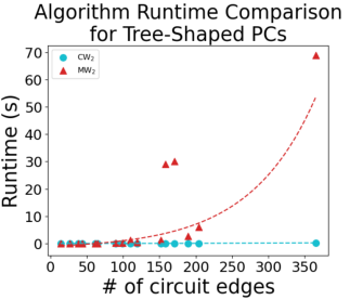
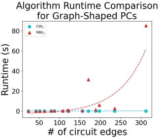
Figure 1: Runtime of Wasserstein-type distance computation using our approach (blue dots) and the baseline (red triangles). For circuits larger than those depicted, the baseline approach runs out of memory. See Appendix C.1 for more detailed experiments.

To determine the feasibility of computing $\textsf{CW}_{p}$ for large circuits, we implement and evaluate our algorithm on randomly-generated compatible circuits of varying sizes. As a baseline, we consider the naive application of an existing algorithm to compute a similar Wasserstein-type distance called “Mixture Wasserstein” $\textsf{MW}_{p}$ between Gaussian mixture models (GMMs) [5], leveraging the fact that PCs with Gaussian input units can be “unrolled” into GMMs. However, we quickly observe the impracticality of this baseline approach for circuits larger than even a few hundred edges due to the GMM representation of a PC potentially being exponentially larger than the original circuit. Figure 1 illustrates how the direct application of GMM-based algorithms is intractable, while our approach runs in quadratic time in the size of the original circuits just as predicted by the theory.

3 Parameter Learning of PCs using the Empirical Wasserstein Distance

Motivated by past works that minimize the Wasserstein distance between a generative model and the empirical distribution, parameterized by a dataset, to train model parameters [14, 15, 16, 1], we investigate the applicability of minimizing the Wasserstein distance between a PC and data as a means of learning the parameters of a given PC structure.

Let $C$ be a PC, and let $D=\{d_{k}\}_{k=1}^{n}$ be a dataset consisting of $n$ i.i.d. samples from some data distribution. First, observe that we can approximate the Wasserstein distance between the circuit and the data distribution as the following by rewriting the expectation as a sum over the dataset and using linearity of expectations:

$$\operatorname{\mathbb{E}}_{\gamma}[\left\lVert\mathbf{X}-\mathbf{Y}\right\rVert_{2}^{2}]\approx\operatorname{\mathbb{E}}_{\gamma}[\frac{1}{n}\sum_{k}\left\lVert\mathbf{X}-d_{k}\right\rVert_{2}^{2}]=\frac{1}{n}\sum_{k=1}^{n}\operatorname{\mathbb{E}}_{\gamma}[\left\lVert\mathbf{X}-d_{k}\right\rVert_{2}^{2}]$$ (3)

Here, $\gamma$ is the optimal coupling between $C$ and the data distribution. Similar to the computation in coupling circuits, the above expectation can be pushed down to the input nodes and computed as a weighted sum at sum nodes and unweighted sum at product nodes (see Appendix B.2). We propose minimizing this expectation above as a way to train circuits, with the intuition being that minimizing this training objective minimizes the Wasserstein distance between the circuit and data distributions.

Our approach builds off the construction of a coupling circuit; similar to how we construct the cross product of sum node children and solve a linear program to get the edge parameters, here we construct a linear program for each sum node to determine how to couple data to the circuit. We propose an iterative algorithm in which we alternate between optimizing the coupling given the current circuit parameters and updating the circuit parameters given the current coupling. Intuitively, sub-circuits with a low expected distance to a lot of points should have a high weight parameter, so a linear program at a sum node with $m$ children and a dataset with $n$ datapoints has $m\times n$ variables $x_{i,j}$, each with objective coefficient $c_{i,j}$ corresponding to the distance between datapoint $j$ and sub-circuit $i$. The constraints enforce that the weight of each datapoint in minimizing the objective is uniform across all data points (so $\sum_{i}x_{i,j}$ is the same regardless of $j$), but we relax the marginal constraints for the circuit since we want to update the circuit’s distribution rather than preserve it. The final node parameters $\theta_{i}$ are retrieved by computing $\sum_{j}x_{i,j}$, and the algorithm continues coupling data at the child nodes in a top-down fashion. A full algorithm is provided in Appendix A.3, and a proof of the the objective function being monotonically decreasing is provided in Appendix B.8.

Conveniently, the above linear program at each sum node is a variation of the continuous knapsack problem [13] and thus has a closed-form solution. In particular, solution results in the coupling with each data point having a weight of either $\frac{1}{n}$ or zero (see Appendix B.7). Due to the closed-form solution of the LP, the time complexity of one iteration of our algorithm is linear in both the size of the circuit and the size of the dataset, and our algorithm is also guaranteed to reach a local minimum for the objective value as every iteration only decreases (or preserves) the empirical Wasserstein objective. Nevertheless, finding the global optimum parameters minimizing the Wasserstein distance is still NP-hard (see Appendix 5), and our proposed efficient algorithm may get stuck at a local minimum, similar to existing maximum-likelihood parameter learning approaches.

3.1 Experimental Results

To determine the performance of our proposed Wasserstein minimization algorithm, we consider learning the parameters of circuits of various sizes from the MNIST benchmark dataset [8]. When compared to mini-batch Expectation Maximization (EM) for estimating maximum-likelihood parameters, our Wasserstein Minimization (WM) approach is nearly competitive for small circuits but falls behind for larger circuits. We attribute this to WM’s inability to make use of the parameter space of larger models. Detailed experimental results are provided in Appendix C.4.

4 Conclusion

This paper studied the optimal transport problem for probabilistic circuits. We introduced a Wasserstein-type distance $\textsf{CW}_{p}$ between two PCs an proposed an efficient algorithm that computes the distance and corresponding optimal transport plan in quadratic time in the size of the input circuits, provided that their circuit structures are compatible. We show that $\textsf{CW}_{p}$ always upper-bounds the true Wasserstein distance, and that—when compared to the naive application of an existing algorithm for computing a Wasserstein-type distance between GMMs to PCs—the former is exponentially faster to compute between circuits. Lastly, we propose an iterative algorithm to minimize the empirical Wasserstein distance between a circuit and data, suggesting an alternative, viable approach to parameter estimation for PCs which is mainly done using maximum-likelihood estimation. While performance was competitive with the EM algorithm for small circuits, and we leave as future work to get Wasserstein Minimization to fully exploit the increased expressiveness of larger models.

We consider this work an initial stepping stone towards a deeper understanding of optimal transport theory for probabilistic circuits. Future work includes exploring more expressive formulations of coupling circuits to close the gap between $\textsf{CW}_{p}$ and $\textsf{MW}_{p}$, extending the marginal-preserving properties of coupling circuits to the multimarginal setting, and computing Wasserstein barycenters for PCs.

Appendix A Algorithms

A.1 Algorithm for Computing the Coupling Circuit between PCs

Algorithm 1 details the construction of a coupling circuit and the computation of the optimal parameters for sum nodes. LP represents a linear program and we assume that sum nodes in $n_{1}$ have $i$ children and sum nodes in $n_{2}$ have $j$ children. With caching of both $\textsf{CW}_{p}(n)$ and $\textsc{Couple}(n_{1},n_{2})$ calls, this algorithm runs in quadratic time.

Algorithm 1 Couple$(n_{1},n_{2})$: couples circuits rooted at $n_{1}$ and $n_{2}$.

$n\leftarrow\text{cache}(n_{1},n_{2})$ 

if $n\neq null$ then

     return $n$

end if

if $n_{1},n_{2}$ are input nodes then

     $n\leftarrow$ new product($n_{1},n_{2}$)

else if $n_{1},n_{2}$ are sum nodes then

     $n\leftarrow$ new sum node  $\triangleright$ will have $i\times j$ children

     $\textsc{LP}\leftarrow$ new linear program with variables $\theta_{i,j}$ $\triangleright$ has $i\times j$ variables

     for $c_{1}\in n_{1}$.children do

         for $c_{2}\in n_{2}$.children do

              $n.$children$[i,j]\leftarrow\textsc{Couple}(c_{1},c_{2})$ $\triangleright$ set child subcircuits

         end for

     end for

     for $\theta_{i}\in n_{1}$.parameters do

         LP.constraints $\leftarrow\sum_{j}\theta_{i,j}=\theta_{i}$ $\triangleright$ add marginal constraints

     end for

     for $\theta_{j}\in n_{2}$.parameters do

         LP.constraints $\leftarrow\sum_{i}\theta_{i,j}=\theta_{j}$ $\triangleright$ add marginal constraints

     end for

     LP.objective $\leftarrow\sum_{i,j}\theta_{i,j}\cdot\textsf{CW}_{p}(c_{i},c_{j})$ $\triangleright$ set objective of linear program

     solve LP

     $n$.parameters $\leftarrow$ optimal parameters from LP

else if $n_{1},n_{2}$ are product nodes then

     $n\leftarrow$ new product node

     for $c_{1}\in n_{1}.$children, $c_{2}\in n_{2}$.children where $\textsf{sc}(c_{1})=\textsf{sc}(c_{2})$ do

         $n$.children.insert$(\textsc{Couple}(c_{1},c_{2}))$ $\triangleright$ couple corresponding children

     end for

end if

cache$(n_{1},n_{2})\leftarrow n$

return $n$

A.2 Algorithm for Computing the Wasserstein Objective for a Coupling Circuit

Given a coupling circuit rooted at $n$, Algorithm 2 computes the value of the Wasserstein objective (see Definition 1) for the coupling. With caching, this algorithm runs in linear time.

Algorithm 2 $\textsf{CW}_{p}(n)$: $p$-Wasserstein objective for a coupling circuit rooted at $n$ with $i$ children.

if $n$ is a product node with input node children then

     return $\textsf{W}_{p}(n.$children[0]$,n$.children[1])

else if $n$ is a product node without input node children then

     return $\sum_{i}\textsf{CW}_{p}(n.$children[$i$])

else if $n$ is a sum node then

     return $\sum_{i}\theta_{i}\textsf{CW}_{p}(n.$children[$i$])

end if

A.3 Algorithm for Minimum Wasserstein Parameter Estimation

Our proposed algorithm is broadly divided into two steps: an inference step and a minimization step. These steps are performed iteratively until model convergence. The inference step populates a cache, which stores the expected distance of each data point at each node in the circuit. This inference step is done in linear time in a bottom-up recursive fashion, making use of the cache for already-computed results. This is provided in algorithm 3.

The minimization step is done top-down recursively, and seeks to route the data at a node to its children in a way that minimizes the total expected distance between the routed data at each child and the sub-circuit. The root node is initialized with all data routed to it. At a sum node, each data point is routed to the child that has the smallest expected distance to it (making use of the cache from the inference step), and the edge weight corresponding to a child is equal to the proportion of data routed to that child; at a product node, the data point is routed to both children. Input node parameters are updated to reflect the empirical distribution of the data routed to that node. The minimization step is thus also done in linear time, and we note that this algorithm guarantees a non-decreasing objective function (see Appendix B.8 for a proof). The algorithm for this is provided in algorithm 4.

Algorithm 3 Inference$(n,D)$: returns a cache storing the distance between each datapoint $d_{j}\in D$ and each sub-circuit rooted at $n$, where $n$ has children $c_{i}$. For conciseness, we omit checking for cache hits

for $c_{i}\in n$.children do

     Inference$(c_{i},D)$ $\triangleright$ recursively build cache

end for

if $n$ is a product node then

     for $d_{j}\in D$ do

         cache$[n,d_{j}]\leftarrow\sum_{i}$cache$[c_{i},d_{j}]$

     end for

end if

if $n$ is a sum node then

     for $d_{j}\in D$ do

         cache$[n,d_{j}]\leftarrow\sum_{i}\theta_{i}$cache$[c_{i},d_{j}]$

     end for

end if

if $n$ is an input node then

     for $d_{j}\in D$ do

         cache$[n,d_{j}]\leftarrow dist(n,d_{j})$ $\triangleright$ here, $dist(n,d_{j})$ is the expected distance between $n$ and $d_{j}$

     end for

end if

return cache

Algorithm 4 Learn$(n,D,\text{cache})$: learns the parameters of circuit rooted at $n$ on datapoints $d_{j}\in D$

if not all parents of $n$ have been learned then

     return $\triangleright$ We only call this method on nodes who’s parents have all been learned

end if

if $n$ is a product node then

     for $c_{i}\in n.$children do

         $[c_{i}]\leftarrow\text{routing}[n]$ $\triangleright$ products route their data to their children

     end for

else if $n$ is a sum node then

     $\forall\theta_{i},$ $\theta_{i}\leftarrow 0$ $\triangleright$ zero out parameters

     for $d_{j}\in\text{routing}[n]$ do $\triangleright$ route data points at current node to children

         $c_{i}\leftarrow\arg\min_{c_{i}}\text{ cache}[c_{i},d_{j}]$ $\triangleright$ $c_{i}$ is the child node of $n$ for which $d_{j}$ has the lowest distance

         routing[$c_{i}$] $\leftarrow d_{j}$ $\triangleright$ route $d_{j}$ to $c_{i}$

         $\theta_{i}\leftarrow\theta_{i}+\frac{1}{|\text{routing}[n]|}$ $\triangleright$ update parameter weight

     end for

else if $n$ is an input node then

     $n$.parameters $\leftarrow$ parameters matching empirical distribution of routing$[n]$

end if

Appendix B Proofs

B.1 Hardness Proof of the $\infty$-Wasserstein Distance Between Circuits

Theorem 2

Suppose $P$ and $Q$ are probabilistic circuits over $n$ Boolean variables. Then computing the $\infty$-Wasserstein distance between $P$ and $Q$ is coNP-hard, even when $P$ and $Q$ are deterministic and structured-decomposable.

Proof 1

We will prove hardness by reducing the problem of deciding equivalence of two DNF formulas, which is known to be coNP-hard, to Wasserstein distance computation between two compatible PCs.

Consider a DNF $\alpha$ containing $m$ terms $\{\alpha_{1},\dots,\alpha_{m}\}$ over Boolean variables $\mathbf{X}$. We will construct a PC $P_{\alpha}$ associated with this DNF as follows. For each term $\alpha_{i}$, we construct a product of input nodes—one for each $X\in\mathbf{X}$ whose literal appears in term $\alpha_{i}$, $\mathds{1}[X=1]$ for a positive literal and $\mathds{1}[X=0]$ for negative. Then we construct a sum unit with uniform parameters over these products as the root of our PC: $P_{\alpha}=\sum_{i=1}^{m}\frac{1}{m}P_{\alpha_{i}}$. We can easily smooth this PC by additionally multiplying $P_{\alpha_{i}}$ with a sum node $\frac{1}{2}\mathds{1}[X=0]+\frac{1}{2}\mathds{1}[X=1]$ for each variable $X$ that does not appear in $\alpha_{i}$. Furthermore, note that every product node in this circuit fully factorizes the variables $\mathbf{X}$, and thus the PC is trivially compatible with any decomposable circuit over $\mathbf{X}$ and in particular with any other PC for a DNF over $\mathbf{X}$, constructed as above.

Clearly, the above PC $P_{\alpha}$ assigns probability mass only to the models of $\alpha$. In other words, for any $\mathbf{x}\in\{0,1\}^{n}$, $P_{\alpha}(\mathbf{x})>0$ iff $\mathbf{x}\models\alpha$ (i.e. there is a term $\alpha_{i}$ that is satisfied by $\mathbf{x}$).

B.2 Recursive Computation of the Wasserstein Objective

Referring to Definition 1, the Wasserstein objective for a given coupling circuit $C(\mathbf{x},\mathbf{y})$ is the expected distance between $\mathbf{x}$ and $\mathbf{y}$. Below, we demonstrate that the Wasserstein objective at a sum node that decomposes into $C(\mathbf{x},\mathbf{y})=\sum_{i}\theta_{i}C_{i}(\mathbf{x},\mathbf{y})$ is simply the weighted sum of the Wasserstein objectives at its children:

$$\operatorname{\mathbb{E}}_{C(\mathbf{x},\mathbf{y})}[\left\lVert\mathbf{x}-\mathbf{y}\right\rVert_{p}^{p}]=\int\left\lVert\mathbf{x}-\mathbf{y}\right\rVert_{p}^{p}C(\mathbf{x},\mathbf{y})d\mathbf{x}d\mathbf{y}=\int\left\lVert\mathbf{x}-\mathbf{y}\right\rVert_{p}^{p}\sum_{i}\theta_{i}C_{i}(\mathbf{x},\mathbf{y})d\mathbf{x}d\mathbf{y}$$

$$=\sum_{i}\theta_{i}\int\left\lVert\mathbf{x}-\mathbf{y}\right\rVert_{p}^{p}C_{i}(\mathbf{x},\mathbf{y})d\mathbf{x}d\mathbf{y}=\sum_{i}\theta_{i}\operatorname{\mathbb{E}}_{C_{i}(\mathbf{x},\mathbf{y})}[\left\lVert\mathbf{x}-\mathbf{y}\right\rVert_{p}^{p}]$$ (4)

Now, consider a decomposable product node, where $C(\mathbf{x},\mathbf{y})=C_{1}(\mathbf{x}_{1},\mathbf{y}_{1})C_{2}(\mathbf{x}_{2},\mathbf{y}_{2})$ . Below, we see that the Wasserstein objective at the parent is simply the sum of the Wasserstein objectives at its children:

$$\operatorname{\mathbb{E}}_{C(\mathbf{x},\mathbf{y})}[\left\lVert\mathbf{x}-\mathbf{y}\right\rVert_{p}^{p}]=\int\left\lVert\mathbf{x}-\mathbf{y}\right\rVert_{p}^{p}C(\mathbf{x},\mathbf{y})d\mathbf{x}d\mathbf{y}=\int\left\lVert\mathbf{x}-\mathbf{y}\right\rVert_{p}^{p}C_{1}(\mathbf{x}_{1},\mathbf{y}_{1})C_{2}(\mathbf{x}_{2},\mathbf{y}_{2})d\mathbf{x}d\mathbf{y}$$

$$=\int(\left\lVert\mathbf{x}_{1}-\mathbf{y}_{1}\right\rVert_{p}^{p}+\left\lVert\mathbf{x}_{2}-\mathbf{y}_{2}\right\rVert_{p}^{p})\times C_{1}(\mathbf{x}_{1},\mathbf{y}_{1})C_{2}(\mathbf{x}_{2},\mathbf{y}_{2})d\mathbf{x}_{1}d\mathbf{x}_{2}d\mathbf{y}_{1}d\mathbf{y}_{2}$$

$$=\left(\int\left\lVert\mathbf{x}_{1}-\mathbf{y}_{1}\right\rVert_{p}^{p}C_{1}(\mathbf{x}_{1},\mathbf{y}_{1})d\mathbf{x}_{1}d\mathbf{y}_{1}\right)+\left(\int\left\lVert\mathbf{x}_{2}-\mathbf{y}_{2}\right\rVert_{p}^{p})C_{2}(\mathbf{x}_{2},\mathbf{y}_{2})d\mathbf{x}_{2}d\mathbf{y}_{2}\right)$$

$$=\operatorname{\mathbb{E}}_{C_{1}(\mathbf{x}_{1},\mathbf{y}_{1})}[\left\lVert\mathbf{x}_{1}-\mathbf{y}_{1}\right\rVert_{p}^{p}]+\operatorname{\mathbb{E}}_{C_{2}(\mathbf{x}_{2},\mathbf{y}_{2})}[\left\lVert\mathbf{x}_{2}-\mathbf{y}_{2}\right\rVert_{p}^{p}]$$ (5)

Thus, we can push computation of Wasserstein objective down to the leaf nodes of a coupling circuit.

B.3 Proof of the Metric Properties of $\textsf{CW}_{p}$

Proposition 2 (Metric Properties of $\textsf{CW}_{p}$)

For any set $\mathcal{C}$ of compatible circuits, $\textsf{CW}_{p}$ defines a metric on $\mathcal{C}$

Proof 2

It is clear that $\textsf{CW}_{p}$ is symmetric since construction of the coupling circuit is symmetric. Furthermore, since $\textsf{CW}_{p}$ upper-bounds $\textsf{W}_{p}$, it must also be non-negative.

If $\textsf{CW}_{p}(P,Q)=0$, then $\textsf{W}_{p}(P,Q)=0$ so $P=Q$. Any constraint-satisfying assignment of the parameters of a coupling circuit between $P$ and $P$ would also result in the Wasserstein objective at the root node being $0$, since the base-case computation of $\textsf{W}_{p}$ at the leaf nodes would always be zero.

Now, we show that $\textsf{CW}_{p}$ satisfies the triangle inequality. Let $P,Q,R\in\mathcal{C}$ be compatible PCs over random variables $\mathbf{X},\mathbf{Y},$ and $\mathbf{Z},$ and let $d_{1}=\textsf{CW}_{p}(P,Q),\text{ }d_{2}=\textsf{CW}_{p}(P,R),$ and $d_{3}=\textsf{CW}_{p}(R,Q)$ with optimal coupling circuits $C_{1},C_{2},$ and $C_{3}$. We can construct circuits $C_{2}(\mathbf{x}|\mathbf{z})$ and $C_{3}(\mathbf{y}|\mathbf{z})$ that are still compatible with $C_{2}$ and $C_{3}$, since conditioning a circuit preserves the structure. Because all of these are compatible, we can then construct circuit $C(\mathbf{X},\mathbf{Y},\mathbf{Z})=C_{2}(\mathbf{X}|\mathbf{Z})C_{3}(\mathbf{Y}|\mathbf{Z})R(\mathbf{Z})$. Thus, $C$ is a coupling circuit of $P,Q$, and $R$ such that $C_{2}(\mathbf{x},\mathbf{y})=\int C(\mathbf{x},\mathbf{y},\mathbf{z})d\mathbf{z}$ and $C_{3}(\mathbf{y},\mathbf{z})=\int C(\mathbf{x},\mathbf{y},\mathbf{z})d\mathbf{x}$. Then we have:

$$\textsf{CW}_{p}(P,Q) =\int\left\lVert\mathbf{x}-\mathbf{y}\right\rVert_{p}^{p}C_{1}(\mathbf{x},\mathbf{y})d\mathbf{x}d\mathbf{y}=\int\left\lVert(\mathbf{x}-\mathbf{z})-(\mathbf{y}-\mathbf{z})\right\rVert_{p}^{p}C(\mathbf{x},\mathbf{y},\mathbf{z})d\mathbf{x}d\mathbf{y}d\mathbf{z}$$

$$\leq\int\left\lVert\mathbf{x}-\mathbf{z}\right\rVert_{p}^{p}C_{2}(\mathbf{x},\mathbf{z})d\mathbf{x}d\mathbf{z}+\int\left\lVert\mathbf{z}-\mathbf{y}\right\rVert_{p}^{p}C_{3}(\mathbf{y},\mathbf{z})d\mathbf{y}d\mathbf{z}$$

$$=\textsf{CW}_{p}(P,R)+\textsf{CW}_{p}(R,Q)$$

Thus, $\textsf{CW}_{p}$ satisfies the triangle inequality, which concludes the proof.

B.4 Proof of the Optimality of Coupling Circuit Parameter Learning in A.1

Theorem 3

Suppose $P$ and $Q$ are compatible probabilistic circuits with coupling circuit $C$. Then the parameters of $C$ - and thus $\textsf{CW}_{p}$ - can be computed exactly in a bottom-up recursive fashion.

Proof 3

We will construct a recursive argument showing that the optimal parameters of $C$ can be computed exactly. Let $n\in C$ be some non-input node in the coupling circuit $C$ that is the product of nodes $n_{1}$ and $n_{2}$ in $P$ and $Q$ respectively. Then we have three cases:

Case 1: $n$ is a product node with input node children

Due to the construction of the coupling circuit, $n$ must have two children that are input nodes with scopes $\mathbf{X}_{k}$ and $\mathbf{Y}_{k}$. Thus, $\textsf{CW}_{p}(n)$ is simply computed in closed-form as the $p$-Wasserstein distance between the input distributions.

Case 2: $n$ is a product node with non-input node children

By recursion, $\textsf{CW}_{p}(n)=\sum_{i}\textsf{CW}_{p}(c_{i})$ for each child $c_{i}$ of $n$ (see 5).

Case 3: $n$ is a sum node

Let $\theta_{i,j}$ be the parameter corresponding to the product of the $i$-th child of $n_{1}$ and $j$-th child of $n_{2}$. We want to solve the following optimization problem $\inf\operatorname{\mathbb{E}}_{P_{n}(\mathbf{X},\mathbf{Y})}[\left\lVert\mathbf{X}-\mathbf{Y}\right\rVert_{p}^{p}]$, which can be rewritten as follows:

$$\inf\operatorname{\mathbb{E}}_{P_{n}(\mathbf{X},\mathbf{Y})}[\left\lVert\mathbf{X}-\mathbf{Y}\right\rVert_{p}^{p}]=\inf\int_{\mathbb{R}^{d}\times\mathbb{R}^{d}}\left\lVert\mathbf{X}-\mathbf{Y}\right\rVert_{p}^{p}P_{n}(\mathbf{X},\mathbf{Y})d\mathbf{X}d\mathbf{Y}$$ (6)

Rewriting the distribution of $n$ as a mixture of its child distributions $c_{i,j}$, we get:

$$=\inf_{\theta,P_{i,j}}\int_{\mathbb{R}^{d}\times\mathbb{R}^{d}}\left\lVert\mathbf{X}-\mathbf{Y}\right\rVert_{p}^{p}\sum_{i,j}\theta_{i,j}P_{c_{i,j}}(\mathbf{X},\mathbf{Y})d\mathbf{X}d\mathbf{Y}$$ (7)

Due to linearity of integrals, we can bring out the sum:

$$=\inf_{\theta,P_{i,j}}\sum_{i,j}\theta_{i,j}\int_{\mathbb{R}^{d}\times\mathbb{R}^{d}}\left\lVert\mathbf{X}-\mathbf{Y}\right\rVert_{p}^{p}P_{c_{i,j}}(\mathbf{X},\mathbf{Y})d\mathbf{X}d\mathbf{Y}$$ (8)

Lastly, due to the acyclicity of PCs, we can separate out $\inf_{\theta_{i},P_{i,j}}$ into $\inf_{\theta_{i}}\inf_{P_{i,j}}$ and push the latter infimum inside the sum.

$$=\inf_{\theta}\sum_{i,j}\theta_{i,j}(\inf_{P_{i,j}}\int_{\mathbb{R}^{d}\times\mathbb{R}^{d}}\left\lVert\mathbf{X}-\mathbf{Y}\right\rVert_{p}^{p}P_{c_{i,j}}(\mathbf{X},\mathbf{Y})d\mathbf{X}d\mathbf{Y})$$ (9)

Thus, we can solve the inner optimization problem first (corresponding to the optimization problems at the children), and then the outer problem (the optimization problem at the current node). Therefore, a bottom-up recursive algorithm is exact.

B.5 Proof of the Marginal-Matching Properties of Coupling Circuits

Theorem 4

Let $P$ and $Q$ be compatible PCs. Then any feasible coupling circuit $C$ as defined in Def. 4 matches marginals to $P$ and $Q$.

Proof 4

We will prove this by induction. Our base case is two corresponding input nodes $n_{1},n_{2}\in P,Q$. The sub-circuit in $C$ rooted at the product of $n_{1}$ and $n_{2}$ is a product node with copies of $n_{1}$ and $n_{2}$ as children, which clearly matches marginals to $n_{1}$ and $n_{2}$.

Now, let $n_{1}$ and $n_{2}$ be arbitrary corresponding nodes in $P$ and $Q$, and assume that the product circuits for all children of the two nodes match marginals. We then have two cases:

Case 1: $n_{1},n_{2}$ are product nodes

Since the circuits are compatible, we know that $n_{1}$ and $n_{2}$ have the same number of children - let the number of children be $k$. Thus, let $c_{1,i}$ represent the $i$’th child of $n_{1}$, and let $c_{2,i}$ represent the $i$’th child of $n_{2}$. The coupling circuit of $n_{1}$ and $n_{2}$ (denoted $n$) is a product node with $k$ children, where the $i$’th child is the coupling circuit of $c_{1,i}$ and $c_{2,i}$ (denoted $c_{i}$).

By induction, the distribution $P_{c_{i}}(\mathbf{X},\mathbf{Y})$ at each child coupling sub-circuit matches marginals to the original sub-circuits: $P_{c_{i}}(\mathbf{X})=P_{c_{1,i}}(\mathbf{X})$, and $P_{c_{i}}(\mathbf{Y})=P_{c_{2,i}}(\mathbf{Y})$. $n_{1}$ and $n_{2}$ being product nodes means that $P_{n_{1}}(\mathbf{X})=\prod_{i}P_{c_{1,i}}(\mathbf{X})$ and $P_{n_{2}}(\mathbf{Y})=\prod_{i}P_{c_{2,i}}(\mathbf{Y})$, so thus $P_{n}(\mathbf{X})=\prod_{i}P_{c_{i}}(\mathbf{X})=\prod_{i}P_{c_{1,i}}(\mathbf{X})$ and $P_{n}(\mathbf{Y})=\prod_{i}P_{c_{i}}(\mathbf{Y})=\prod_{i}P_{c_{2,i}}(\mathbf{Y})$. Therefore, $n$ matches marginals to $n_{1}$ and $n_{2}$.

Case 2: $n_{1},n_{2}$ are sum nodes

Let the number of children of $n_{1}$ be $k_{1}$ and the number of children of $n_{2}$ be $k_{2}$. Let $c_{1,i}$ represent the $i$’th child of $n_{1}$, and let $c_{2,j}$ represent the $j$’th child of $n_{2}$. The coupling circuit of $n_{1}$ and $n_{2}$ (denoted $n$) is a sum node with $k_{1}*k_{2}$ children, where the $(i,j)$’th child is the coupling circuit of $c_{1,i}$ and $c_{2,j}$ (denoted $c_{i,j}$).

By induction, the distribution $P_{c_{i,j}}(\mathbf{X},\mathbf{Y})$ at each child coupling sub-circuit matches marginals to the original sub-circuits: $P_{c_{i,j}}(\mathbf{X})=P_{c_{1,i}}(\mathbf{X})$, and $P_{c_{i,j}}(\mathbf{Y})=P_{c_{2,j}}(\mathbf{Y})$. $n_{1}$ and $n_{2}$ being sum nodes means that $P_{n_{1}}(\mathbf{X})=\sum_{i}\theta_{i}P_{c_{1,i}}(\mathbf{X})$ and $P_{n_{2}}(\mathbf{Y})=\sum_{j}\theta_{j}P_{c_{2,j}}(\mathbf{Y})$, so thus

$$P_{n}(\mathbf{X})=\sum_{i}\sum_{j}\theta_{i,j}P_{c_{i,j}}(\mathbf{X})=\sum_{i}\sum_{j}\theta_{i,j}P_{c_{1,i}}(\mathbf{X})=\sum_{i}\theta_{i}P_{c_{1,i}}(\mathbf{X})=P_{n_{1}}(\mathbf{X})\\ P_{n}(\mathbf{Y})=\sum_{i}\sum_{j}\theta_{i,j}P_{c_{i,j}}(\mathbf{Y})=\sum_{i}\sum_{j}\theta_{i,j}P_{c_{2,j}}(\mathbf{Y})=\sum_{j}\theta_{j}P_{c_{2,j}}(\mathbf{Y})=P_{n_{2}}(\mathbf{Y})$$ (10)

Note that we rewrite $\sum_{i}\theta_{i,j}=\theta_{j}$ and $\sum_{j}\theta_{i,j}=\theta_{i}$ by the constraints on coupling circuits. Therefore, $n$ satisfies marginal constraints.

B.6 Proving that Computing Minimum Wasserstein Parameters is NP-Hard

Theorem 5

Computing the parameters of probabilistic circuit $C$ is NP-hard.

Proof 5

We will prove this hardness result by reducing $k$-means clustering - which is known to be NP-hard [4] - to learning the minimum Wasserstein parameters of a circuit. Consider a set of points $x_{1}...x_{n}\in\mathbb{R}^{d}$ and a number of clusters $k$. We will construct a Gaussian PC $C$ associated with this problem as follows: the root of $C$ is a sum node with $k$ children; each child is a product node with $d$ univariate Gaussian input node children (so each product node is a multivariate Gaussian comprised of independent univariate Gaussians). Minimizing the parameters of $C$ over $x_{i}$ corresponds to finding a routing of data points $x_{i}$ that minimizes the total distance between all $x_{i}$’s and the mean of the multivariate Gaussian child each $x_{i}$ is routed to. A solution to $k$-means can be retrieved by taking the mean of each child of the root sum node to be the center of each of $k$ clusters.

B.7 Deriving a Closed-Form Solution to the Linear Programs for Parameter Updates

For a sum node $s$ with $m$ children $s_{1}...s_{m}$ and a dataset with $n$ datapoints $d_{1}...d_{n}$ each with weight $w_{j}$, we construct a linear program with $m*n$ variables $x_{i,j}$ as follows:

$$\text{min}\quad\sum_{i=1}^{m}\sum_{j=1}^{n}\operatorname{\mathbb{E}}_{s_{i}}[\left\lVert\mathbf{X}-d_{j}\right\rVert_{2}^{2}]x_{i,j}\qquad\text{s.t.}\quad\sum_{i=1}^{m}x_{i,j}=w_{j}\text{ }\forall j$$

Note that the constraints do not overlap for differing values of $j$. Thus, we can break this problem up into $n$ smaller linear programs, each with the following form:

$$\text{min}\quad\sum_{i=1}^{m}\operatorname{\mathbb{E}}_{s_{i}}[\left\lVert\mathbf{X}-d_{j}\right\rVert_{2}^{2}]x_{i,j}\qquad\text{s.t.}\quad\sum_{i=1}^{m}x_{i,j}=w_{j}$$

The only constraint here requires that the sum of objective variables is equal to $w_{j}$. Thus, the objective is minimized when $x_{i,j}$ corresponding to the smallest coefficient takes value $w_{j}$ and all other variables take value 0. Thus, the solution to the original linear program can be thought of as assigning each data point to the sub-circuit that has the smallest expected distance to it.

B.8 Proof that the Wasserstein Minimization Algorithm has a Monotonically Decreasing Objective

Theorem 6

For a circuit rooted at $n$ and dataset $D$ routed to it, the Wasserstein distance between the empirical distribution of $D$ and sub-circuit rooted at $n$ will not increase after an iteration of algorithm A.3

Proof 6

Let $\operatorname{\mathbb{E}}_{n}[D]$ denote the Wasserstein distance between the empirical distribution of $D$ and sub-circuit rooted at $n$ before an iteration of algorithm A.3, and let $\operatorname{\mathbb{E}}_{n^{\prime}}[D]$ denote the distance after an iteration. We will show by induction that $\operatorname{\mathbb{E}}_{n^{\prime}}[D]\leq\operatorname{\mathbb{E}}_{n}[D]$. Our base case is when $n$ is an input node. By setting the parameters of $n$ to as closely match the empirical distribution of $D$ as possible, there is no parameter assignment with a lower Wasserstein distance to $D$ so thus one iteration of algorithm A.3 does not increase the objective value.

Recursively, we have two cases:

Case 1: $n$ is a product node

By the decomposition of the Wasserstein objective, we have that $\operatorname{\mathbb{E}}_{n}[D]=\sum_{i}\operatorname{\mathbb{E}}_{c_{i}}[D]$, which is $\geq\sum_{i}\operatorname{\mathbb{E}}_{c_{i}^{\prime}}[D]=\operatorname{\mathbb{E}}_{n^{\prime}}[D]$ by induction.

Case 2: $n$ is a sum node

By the decomposition of the Wasserstein objective, we have that $\operatorname{\mathbb{E}}_{n}[D]=\sum_{i}\theta_{i}\operatorname{\mathbb{E}}_{c_{i}}[D_{i}]$ (where $D_{i}\subseteq D$ is the data routed to $n_{i}$), which is $\geq\sum_{i}\theta_{i}\operatorname{\mathbb{E}}_{c_{i}^{\prime}}[D_{i}]=\operatorname{\mathbb{E}}_{n^{\prime}}[D]$ by induction. Our parameter updates also update each $D_{i}\rightarrow D_{i}^{\prime}$, but that also guarantees that $\operatorname{\mathbb{E}}_{c_{i}^{\prime}}[D_{i}]\geq\operatorname{\mathbb{E}}_{c_{i}^{\prime}}[D_{i}^{\prime}]$ since $D_{i}=D_{i}^{\prime}$ is within the feasible set of updates for $D_{i}$. Thus, $\operatorname{\mathbb{E}}_{n}[D]\geq\operatorname{\mathbb{E}}_{n^{\prime}}[D]$, so therefore the Wasserstein objective is monotonically decreasing.

Appendix C Additional Experimental Results

C.1 Additional $\textsf{CW}_{p}$ Runtime Results

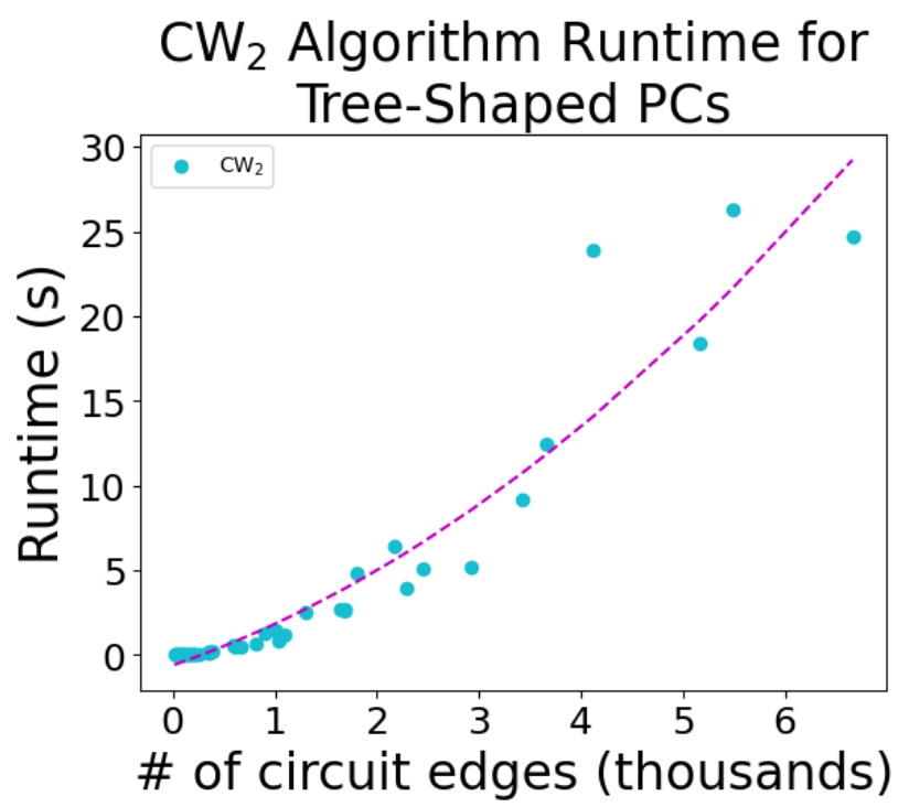
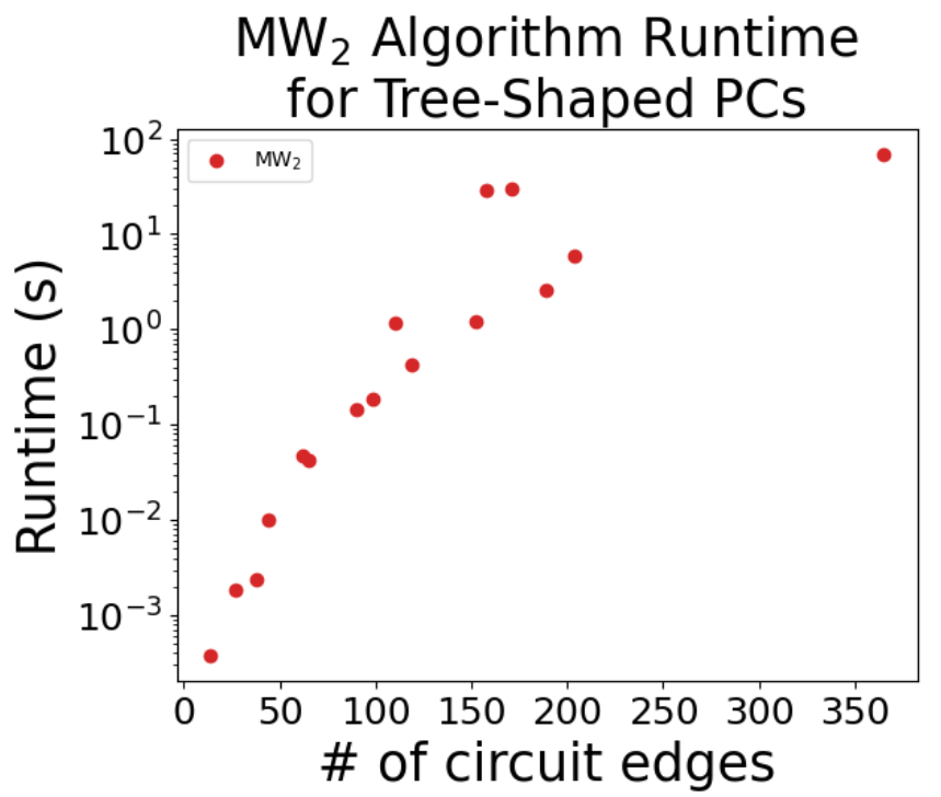
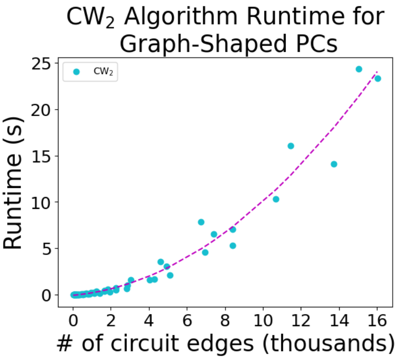
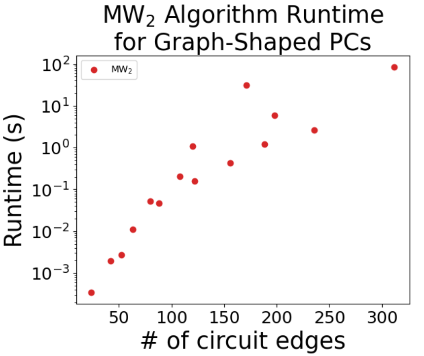
Figure 2: Runtime for algorithms computing $\textsf{CW}_{2}$ and $\textsf{MW}_{2}$. The first pair of graphs considers only tree-shaped PCs, whereas the second pair considers graph-shaped PCs as well. Note that the right-side graphs use logarithmic scaling. Number of circuit edges represents the number of edges in both circuits combined, and each data point represents an average over 100 runs.

To evaluate the runtime of computing $\textsf{CW}_{2}$, we consider a fixed variable scope and randomly construct a balanced region tree for the scope. Then, we randomly construct two PCs for this region tree; the PCs are constructed with a fixed sum node branching factor and fixed rejoin probability - which is the chance that a graph connection to an existing node in the PC will be made to add a child rather than creating a new node for the child, and is 0% in the case of trees and 50% in the case of graphs. We implement our algorithm as detailed in appendix A.1 to compute the optimal transport map and value for $\textsf{CW}_{2}$, as well as also implement a PC-to-GMM unrolling algorithm and the algorithm proposed by [2] to compute $\textsf{MW}_{2}$ [5]. The value obtained for each circuit size is averaged over 100 runs, and we omit data points for experiments that ran out of memory. See Figure 2 for the graphs.

The experiments were conducted on a machine with an Intel Core i9-10980XE CPU and 256Gb of RAM (these experiments made no use of GPUs); linear programs were solved using Gurobi [7]. Each experiment was conducted with a fixed random seed, and the parameter values for sum nodes were clamped to be greater than 0.01 for numeric stability.

C.2 Comparing $\textsf{CW}_{2}$ and $\textsf{MW}_{2}$

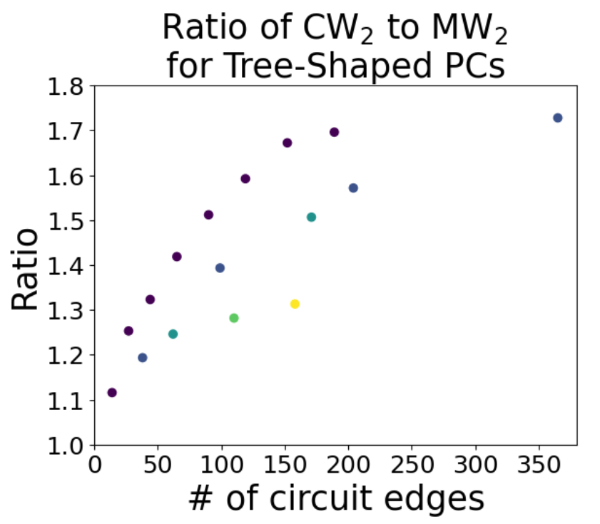
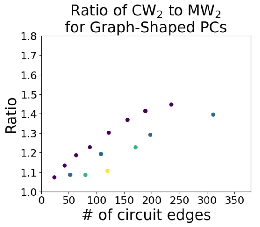
Figure 3: Ratio of $\frac{\textsf{CW}_{2}}{\textsf{MW}_{2}}$, lower is better. Empirically, the gap between $\textsf{CW}_{2}$ and $\textsf{MW}_{2}$ grows roughly linearly in the size of the circuit. The hue of each point represents the circuit depth, with lighter points being a higher depth. Circuit depth does not seem to affect the ratio significantly.

To evaluate the proximity of $\textsf{CW}_{2}$ to $\textsf{MW}_{2}$, we adopt the same framework as we did for runtime experiments to randomly construct compatible PCs and compute $\textsf{CW}_{2}$ and $\textsf{MW}_{2}$ between them. Due to the exponential blowup of computing $\textsf{MW}_{2}$ it quickly becomes impractical to compute (see runtime experiments in Appendix C.1); however, we still attempt to provide some empirical insight into the difference between $\textsf{CW}_{p}$ and $\textsf{MW}_{p}$.

We note that the ratio $\frac{\textsf{CW}_{2}}{\textsf{MW}_{2}}$ appears to grow linearly in the size of the circuit; furthermore, for graph-shaped circuits, the ratio is closer to 1 than for tree-shaped circuits. Figure 3 provides an in-depth look at these observations.

C.3 Visualizing Transport Maps between Circuits

Since our algorithm does not only return $\textsf{CW}_{p}$ between two circuits but also the corresponding transport plan, we can visualize the transport of point densities between the two distributions by conditioning the coupling circuit on an assignment of random variables in one circuit. We can similarly visualize the transport map for an arbitrary region in one PC to another by conditioning on the random variable assignments being within said region. See Figure 4 for an example.

Since the transport plan for a single point (or region of points) is itself a PC, we can query it like we would any other circuit; for example, computing maximum a posteriori - which is tractable if the original two circuits are marginal-deterministic [3] - for the transport plan of a point corresponds to the most likely corresponding point in the second distribution for the given point. Because a coupling circuit inherits the structural properties of the original circuit, it is straightforward to understand what queries are and are not tractable for a point transport map.

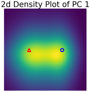
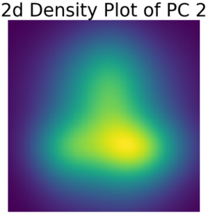
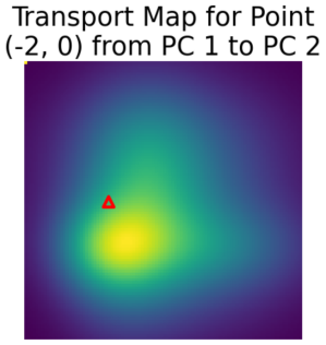
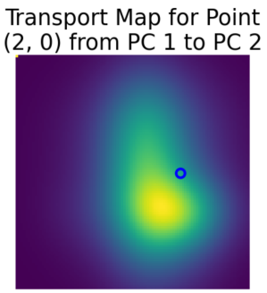
Figure 4: Visualization of transporting the indicated points from the distribution parameterized by PC 1 to the distribution parameterized by PC 2. The top two figures visualize the distributions, while the bottom two figures visualize where the point density indicated is transported to from the first to the second distribution.

C.4 Empirical Wasserstein Parameter Estimation Experimental Results

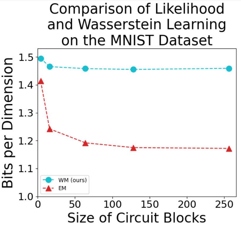
Figure 5: Visualization of the performance of PCs learned using Expectation Maximization (red triangles) and Wasserstein Minimization (our approach, blue dots). The bits-per-dimension (bpd) of the learned circuits does not decrease significantly with an increase in circuit size for circuits learned using the empirical Wasserstein distance.

To understand the effectiveness of parameter estimation via minimizing the empirical Wasserstein distance, we evaluated the performance of PCs trained using the HCLT [11] structure with categorical input distributions on the MNIST [8] dataset. The baseline for this experiment is the EM algorithm for circuits [6].

We first generated the structure of the circuits using the HCLT implementation provided in PyJuice [10], varying the size of each block to increase or decrease the number of parameters. We then learned two sets of circuit parameters per structure per block size: one set of parameters was learned using mini-batch EM with a batch size of 1000, and the other set was learned using an implementation of the algorithm detailed in Appendix A.3. We perform early stopping for the EM algorithm that stops training once the point of diminishing returns has been surpassed. All experiments were ran on a single NVIDIA L40s GPU.

When using bits-per-dimension as a benchmark, we observe that our algorithm performs nearly as well as EM for small circuits (block size of 4). However, as the size of the circuit increases, the performance of our algorithm hardly improves; empirically, our approach to Wasserstein minimization does not make good use of the larger parameter space of larger models, with models that are orders of magnitude larger having better but still comparable performance to their smaller counterparts. We refer to Figure 5 for more details.

References

- [1] Martin Arjovsky, Soumith Chintala, and Léon Bottou. Wasserstein generative adversarial networks. In Doina Precup and Yee Whye Teh, editors, Proceedings of the 34th International Conference on Machine Learning, volume 70 of Proceedings of Machine Learning Research, pages 214–223. PMLR, 06–11 Aug 2017.
- [2] Yongxin Chen, Tryphon T Georgiou, and Allen Tannenbaum. Optimal transport for gaussian mixture models. IEEE Access, 7:6269–6278, 2018.
- [3] YooJung Choi, Antonio Vergari, and Guy Van den Broeck. Probabilistic circuits: A unifying framework for tractable probabilistic models. arXiv preprint, Oct 2020.
- [4] Sanjoy Dasgupta. The hardness of k-means clustering. UCSD Technical Report, 2008.
- [5] Julie Delon and Agnes Desolneux. A wasserstein-type distance in the space of gaussian mixture models. SIAM Journal on Imaging Sciences, 13(2):936–970, 2020.
- [6] Mattia Desana and Christoph Schnörr. Expectation maximization for sum-product networks as exponential family mixture models. arXiv preprint, 04 2016.
- [7] Gurobi Optimization, LLC. Gurobi Optimizer Reference Manual, 2024.
- [8] Yann LeCun, Léon Bottou, Yoshua Bengio, , and Patrick Haffner. Gradient-based learning applied to document recognition. Proceedings of the IEEE, 1998.
- [9] Yitao Liang and Guy Van den Broeck. Towards compact interpretable models : Shrinking of learned probabilistic sentential decision diagrams. In IJCAI 2017 Workshop on Explainable Artificial Intelligence (XAI), 2017.
- [10] Anji Liu, Kareem Ahmed, and Guy Van den Broeck. Scaling tractable probabilistic circuits: A systems perspective, 2024.
- [11] Anji Liu and Guy Van den Broeck. Tractable regularization of probabilistic circuits. In M. Ranzato, A. Beygelzimer, Y. Dauphin, P.S. Liang, and J. Wortman Vaughan, editors, Advances in Neural Information Processing Systems, volume 34, pages 3558–3570. Curran Associates, Inc., 2021.
- [12] Christoph Meinel and Thorsten Theobald. Algorithms and Data Structures in VLSI Design: OBDD-foundations and applications. Springer Science & Business Media, 1998.
- [13] Roberto Tamassia Michael Goodrich. Algorithm Design: Foundations, Analysis, and Internet Examples. John Wiley & Sons, 2002.
- [14] Litu Rout, Alexander Korotin, and Evgeny Burnaev. Generative modeling with optimal transport maps. In International Conference on Learning Representations, 2022.
- [15] Tim Salimans, Dimitris Metaxas, Han Zhang, and Alec Radford. Improving gans using optimal transport. In 6th International Conference on Learning Representations, ICLR 2018, 2018.
- [16] Ilya Tolstikhin, Olivier Bousquet, Sylvain Gelly, and Bernhard Schoelkopf. Wasserstein auto-encoders. In International Conference on Learning Representations, 2018.
- [17] Antonio Vergari, YooJung Choi, Anji Liu, Stefano Teso, and Guy den Broeck. A Compositional Atlas of Tractable Circuit Operations for Probabilistic Inference. In Advances in Neural Information Processing Systems, volume 34, pages 13189–13201, 2021.