Nandan Kumar Jha & Brandon Reagen
New York University
{nj2049, bjr5}@nyu.edu

AERO: Softmax-Only LLMs for Efficient
Private Inference

Nandan Kumar Jha & Brandon Reagen
New York University
{nj2049, bjr5}@nyu.edu

Abstract

The pervasiveness of proprietary language models has raised privacy concerns for users’ sensitive data, emphasizing the need for private inference (PI), where inference is performed directly on encrypted inputs. However, current PI methods face prohibitively higher communication and latency overheads, primarily due to nonlinear operations. In this paper, we present a comprehensive analysis to understand the role of nonlinearities in transformer-based decoder-only language models. We introduce AERO, a four-step architectural optimization framework that refines the existing LLM architecture for efficient PI by systematically removing nonlinearities such as LayerNorm and GELU and reducing FLOPs counts. For the first time, we propose a Softmax-only architecture with significantly fewer FLOPs tailored for efficient PI. Furthermore, we devise a novel entropy regularization technique to improve the performance of Softmax-only models. AERO achieves up to 4.23$\times$ communication and 1.94$\times$ latency reduction. We validate the effectiveness of AERO by benchmarking it against the state-of-the-art.

1 Introduction

Motivation. The widespread adoption of proprietary models like ChatGPT Achiam et al. (2023) significantly raised the privacy concerns to protect the users’ sensitive (prompt) data Staab et al. (2024); Mireshghallah et al. (2024); Priyanshu et al. (2023); Lauren & Knight (2023), while also preventing the attacks aimed at extracting model weights Carlini et al. (2024); Jovanović et al. (2024).

This emphasizes the need for private inference (PI) where a user sends the encrypted queries to the service provider without revealing their actual inputs, and the inference is performed directly on encrypted inputs, assuring the privacy of input and protection of the model’s weight.

Despite their promises, current PI methods remain impractical due to their prohibitive latency and communication overheads—generating a single output token with GPT-2 model (125M parameters) on 128 input tokens takes 8.2 minutes and requires 25.3 GBs communication (Figure 1), scaling to 30.7 minutes and 145.2 GBs for context size of 512 (Table 6). These overheads stem largely from the nonlinear operations, crucial for model performance, in a transformer-based large language model (LLM), such as GELU, LayerNorm, and Softmax Hou et al. (2023); Lu et al. (2025).

Challenges. Current PI solutions for transformer-based models (e.g., ViT, BERT) either neglect the cost of LayerNorm (Li et al., 2023a; Zeng et al., 2023; Zhang et al., 2023; Chen et al., 2023) or approximate nonlinear operations using polynomial functions Zimerman et al. (2024); Dhyani et al. (2024). Nonetheless, polynomial approximation methods have their limitations: their accuracy is highly sensitive to data-specific initial guesses Knott et al. (2021), and their effectiveness is confined to narrow input ranges Zimerman et al. (2024). Moreover, networks employing higher-degree polynomials for improved approximation precision are notoriously difficult to train and optimize.

Meanwhile, the nonlinearity reduction methods, used for improving plaintext speed, offer very-limited potential to improve the PI efficiency. For instance, (He et al., 2023; Noci et al., 2023; He & Hofmann, 2024) has explored architectural heuristics to design LayerNorm-free LLMs; however, their broader implications on the choices of activation function, a key bottleneck in PI, remains largely unexamined.

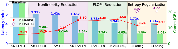
Figure 1: Latency and communication savings through nonlinearity and FLOPs reduction steps when AERO is applied on GPT-2, and trained from scratch on CodeParrot dataset. Further, we benchmark AERO against the SOTA He & Hofmann (2024) at iso-latency points. See Table 3 for a detail analysis.

Our techniques and insights. We conducted an in-depth analysis of the role of non-linearities, specifically GELU and LayerNorm, in transformer-based LLMs. Our key findings are: (1) LayerNorm-free models exhibit a preference for ReLU over GELU in FFN, making them more PI-friendly; and (2) training instability, as entropy collapse in deeper layers, in the Softmax-only model can be prevented by normalizing FFN weights, avoiding the nonlinear computations (unlike LayerNorm) at inference.

We observed a phenomenon we term entropic overload, where a disproportionately larger fraction of attention heads stuck at higher, close to their maximum, entropy values in LN-free with GELU, and Softmax-only models. We hypothesize that the entropic overload causes a lack of diversity and specialization in attention heads, squandering the representational capacity of attention heads. This leads to performance degradation, indicated by a higher perplexity.

To mitigate the entropic overload, we propose a novel entropy regularization technique that penalizes the extreme entropy values at training and avoids the deviation from well-behaved entropy distribution.

Results and implications. As shown in Figure 1, substituting GELU with ReLUs in the baseline GPT-2 model alone reduces the communication and latency overheads by 2.68$\times$ and 1.35$\times$, respectively. Eliminating LayerNroms further improves these savings to 3.41$\times$ and 1.42$\times$. Similar improvements are observed with the Pythia model (see Figure14).

Since the FFN in the Softmax-only model is performing only the linear transformations, merging the linear layers into a single linear layer reduces the FFN FLOPs by 8$\times$ and gains significant speedup without increasing the perplexity (see Figure 1). Furthermore, our analysis reveals that the linear transformations performed by early FFNs are crucial for training stability in the Softmax-only model, while deeper FFNs can be pruned. This provides additional opportunities for FLOPs reduction.

Contributions. Our key contributions are follows:

1. We thoroughly characterize the role of GELU and LayerNorm nonlinearities in transformer-based LLMs by examining their impact on the attention score distribution using Shannon’s entropy, offering insights for tailoring existing LLM architectures for efficient PI.

2. We introduced AERO, a four-stage optimization framework, and designed a Softmax-only model with fewer FLOPs, achieving up to 1.94$\times$ speedup and 4.23$\times$ communication reduction.

3. We introduce a novel entropy regularization technique to boost the performance of the Softmax-only model, which achieves 6% - 8% improvement in perplexity.

4. We conducted extensive experiments across various context sizes (128, 256, 512) and model depths (12L and 18L) on a wide range of training tokens (1.2B to 4.8B) from the CodeParrot Face and Languini dataset Stanić et al. (2023) on GPT-2 and Pythia Biderman et al. (2023) models.

2 Preliminaries

Notations. We denote the number of layers as $L$, number of heads as $H$, model dimensionality as $d$, head dimension as $d_{k}$ (where $d_{k}=\frac{d}{H}$), and context length as $T$. Table 1 illustrates the abbreviations for architectural configurations with simplified nonlinearities in a transformer-based LLM.

An overview of transformer-based decoder-only architecture. A transformer-based LLM is constructed by sequentially stacking $L$ transformer blocks, where each block is composed of two sub-blocks: an attention mechanism and a feed-forward network (FFN), both having their own residual connections and normalization layers, positioned in the Pre-LN order to improves training stability (Xiong et al., 2020). Formally, transformer blocks take an input sequence $\mathbf{X}_{\text{in}}\in\mathbb{R}^{T\times d}$, consisting of $T$ tokens of dimension $d$, and transform it into $\mathbf{X}_{\text{out}}$ as follows:

$$\mathbf{X}_{\text{out}}=\hat{\mathbf{X}}_{\text{SA}}+\text{FFN}_{\text{GELU}}(\text{LayerNorm}_{2}(\hat{\mathbf{X}}_{\text{SA}})),\;\text{where}\;\hat{\mathbf{X}}_{\text{SA}}=\mathbf{X}_{\text{in}}+\text{MHA}(\text{LayerNorm}_{1}(\mathbf{X}_{\text{in}})).$$ (1)

The Multi-Head Attention (MHA) sub-block enables input contextualization by sharing information between individual tokens. MHA employs the self-attention mechanism to compute the similarity score of each token with respect to all other tokens in the sequence. In particular, self-attention mechanism transform the input sequence $\mathbf{X}$ into $\mathbf{Attn}(\mathbf{X})$ as follows:

$$\mathbf{Attn}(\mathbf{X})=\Big{(}\text{Softmax}\Big{(}\frac{1}{\sqrt{d_{k}}}(\mathbf{X}\mathbf{W}^{Q})(\mathbf{X}{\mathbf{W}^{K}})^{\top}+\mathbf{M}\Big{)}\Big{)}\mathbf{X}\mathbf{W}^{V}.$$ (2)

Here, each token generates query($Q$), key($K$), and value($V$) vectors through the linear transformations $\mathbf{W}^{Q},\mathbf{W}^{K},\;\text{and}\;\mathbf{W}^{V}\in\mathbb{R}^{d\times d}$, respectively. Then, similarity scores are computed by taking the dot product of the $Q$ and $K$ vectors, scaled by the inverse square root of the $K$ dimension, and passed through a softmax function to obtain the attention weights. These weights are then used to compute a weighted sum of the $V$ vectors, producing the output for each token. For auto-regressive models (e.g., GPT), mask $\mathbf{M}\in\mathbb{R}^{T\times T}$, which has values in $\{0,-\infty\}$ with $\mathbf{M}_{i,j}=0\,\text{iff}\,{i\geq j}$, is deployed to prevent the tokens from obtaining information from future tokens.

The MHA sub-block employs a self-attention mechanism across all the heads, each with its own sets of $Q$, $K$, and $V$. This allows the attention heads to focus on different parts of the input sequence, capturing various aspects of the input data simultaneously. The outputs from all heads are concatenated and linearly transformed ($\mathbf{W}^{O}\in\mathbb{R}^{d\times d}$) to produce the final MHA output as follows:

$$\text{MHA}(\mathbf{X})=\text{Concat}\big{(}\text{Attn}_{1}(\mathbf{X}),\;\text{Attn}_{2}(\mathbf{X}),\;\text{Attn}_{3}(\mathbf{X}),\dots,\text{Attn}_{H}(\mathbf{X})\big{)}\mathbf{W}^{O}.$$ (3)

Following the MHA sub-block, the FFN sub-block transforms each token independently. The FFN sub-blocks have a single hidden layer whose dimension is a multiple of $d$ (e.g., $4d$ in GPT (Radford et al., 2019) models). Specifically, the FFN sub-block first applies a linear transformation to the input $\mathbf{X}$ using $\mathbf{W}^{\text{ffn}}_{\text{in}}\in\mathbb{R}^{d\times 4d}$, followed by a non-linear transformation using an activation function such as GELU. This is then followed by another linear transformation using $\mathbf{W}^{\text{ffn}}_{\text{out}}\in\mathbb{R}^{4d\times d}$, as follows:

$$\text{FFN}(\mathbf{X})=(\text{GELU}(\mathbf{X}\mathbf{W}^{\text{ffn}}_{\text{in}}))\mathbf{W}^{\text{ffn}}_{\text{out}}$$ (4)

The combination of MHA and FFN sub-blocks, along with residual connections and normalization layers, allows transformer models to learn the contextual relationships between tokens effectively.

Threat model for private inference. We consider the standard two-party (2PC) client-server setting used in PPML, which provides security against semi-honest (honest-but-curious) adversaries bounded by probabilistic polynomial time Zhang et al. (2025); Lu et al. (2025); Pang et al. (2024); Hou et al. (2023). Both parties follow protocol specifications but may attempt to gain additional information from their outputs about the other party’s input. In this 2PC setting, the server holds the propriety GPT model (e.g., ChatGPT), and the client queries the model with a piece of text (prompt). The protocols ensure that the server does not know anything about the client’s input and the output of their queries, and the client does not know anything about the server’s model except its architecture.

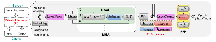
Figure 2: An illustration of threat model and cryptographic protocols used for LLM private inference.

3 Removing Nonlinearity in Transformer-based LLMs

In this section, we investigate the role of non-linearities in the learning dynamics and internal representations of a transformer-based autoregressive decoder-only LLM. We design a controlled experimental framework that systematically removes non-linear components from the architecture (see Table 1), and trains models from scratch.

Table 1: Architectural configurations of nonlinearities in LLMs, illustrating the combinations of Softmax (SM), LayerNorm (LN), GELU (G), and ReLU (R) functions (see Eq. 1, 2, 3 and 4).

Abbreviation	Architectural configuration
SM + LN + G	$\mathbf{X}_{\text{out}}=\text{FFN}_{\text{{\color[rgb]{1,0,0}GELU}}}(\text{{\color[rgb]{.5,0,.5}LayerNorm}}_{{\color[rgb]{.5,0,.5}2}}(\text{MHA}(\text{Attn}_{\text{{\color[rgb]{0,0,1}Softmax}}}(\text{{\color[rgb]{.5,0,.5}LayerNorm}}_{{\color[rgb]{.5,0,.5}1}}(\mathbf{X}_{\text{in}})))))$
SM + LN + R	$\mathbf{X}_{\text{out}}=\text{FFN}_{\text{{\color[rgb]{1,0,0}ReLU}}}(\text{{\color[rgb]{.5,0,.5}LayerNorm}}_{{\color[rgb]{.5,0,.5}2}}(\text{MHA}(\text{Attn}_{\text{{\color[rgb]{0,0,1}Softmax}}}(\text{{\color[rgb]{.5,0,.5}LayerNorm}}_{{\color[rgb]{.5,0,.5}1}}(\mathbf{X}_{\text{in}})))))$
SM + LN	$\mathbf{X}_{\text{out}}=\text{FFN}_{\text{Identity}}(\text{{\color[rgb]{.5,0,.5}LayerNorm}}_{{\color[rgb]{.5,0,.5}2}}(\text{MHA}(\text{Attn}_{\text{{\color[rgb]{0,0,1}Softmax}}}(\text{{\color[rgb]{.5,0,.5}LayerNorm}}_{{\color[rgb]{.5,0,.5}1}}(\mathbf{X}_{\text{in}})))))$
SM + G	$\mathbf{X}_{\text{out}}=\text{FFN}_{\text{{\color[rgb]{1,0,0}GELU}}}(\text{MHA}(\text{Attn}_{\text{{\color[rgb]{0,0,1}Softmax}}}(\mathbf{X}_{\text{in}})))$
SM + R	$\mathbf{X}_{\text{out}}=\text{FFN}_{\text{{\color[rgb]{1,0,0}ReLU}}}(\text{MHA}(\text{Attn}_{\text{{\color[rgb]{0,0,1}Softmax}}}(\mathbf{X}_{\text{in}})))$
SM	$\mathbf{X}_{\text{out}}=\text{FFN}_{\text{Identity}}(\text{MHA}(\text{Attn}_{\text{{\color[rgb]{0,0,1}Softmax}}}(\mathbf{X}_{\text{in}})))$

To analyze internal representations, we use Shannon’s entropy to examine the impacts of nonlinearities on the attention score distribution (see Appendix A.1 for its justification). We highlight key insights and findings, offering practical guidelines for tailoring LLM architectures for efficient PI.

(a) Headwise entropy distribution

(b) Loss curve

figure (a) The fraction of attention heads distributed across different entropy ranges, and (b) evaluation loss for GPT-2 (small) models with fewer nonlinearities, when trained from scratch on CodeParrot dataset.

Configurations	PPL	+$\Delta$(%)
SM + LN + G	2.69	0.00
SM + LN + R	2.76	2.53
SM + LN	3.38	25.58
SM + G	3.20	18.92
SM + R	2.94	9.20
SM	NaNs	-

tableEvaluation perplexity for GPT-2 (small) models with fewer nonlinearities, corresponding to Figure 2bb. $\Delta$ is increase in PPL over baseline network.

Well-behaved entropy distribution We begin by analyzing the headwise entropy distribution of baseline architecture with GELU and ReLU in the FFN, i.e., configurations ${\tt SM+LN+G}$ and ${\tt SM+LN+R}$ respectively. We find that the majority of heads ($\approx$90%) possess entropy values between $\frac{\text{max}}{4}$ and $\frac{\text{3max}}{4}$, where ${\tt max}$ is maximum observed entropy value among all heads (see Figure 2ba). This concentration in the middle entropy range, while avoiding extremes, demonstrates a well-behaved distribution, providing a benchmark for assessing the impact of nonlinearities on model behavior.

Entropic overload We observed that in certain nonlinearity configurations, a disproportionately large fraction of the attention heads exhibit higher entropy values (between $\frac{3\text{max}}{4}$ and ${\tt max}$). We term this phenomenon as entropic overload and hypothesize that this imbalance results in under-utilization of the network’s representational capacity, as too many heads engaged in exploration, hindering the model from effectively leveraging the diversity of attention heads.

To investigate further, we examined how entropy values evolve during training. Typically, all heads start with higher entropy values, indicating an initial exploration phase, and gradually adapt to balance exploration and exploitation in baseline networks (see Figure 11). However, in the absence of certain nonlinearities, this balance is disrupted, preventing attention heads from specializing and refining their focus on critical aspects of the input, thereby diminishing overall performance.

3.1 Desirable Activation Function in LayerNorm-Free LLMs

We first remove LayerNorm from the LLM architecture and study the desirable activation function in this design, as the absence of LayerNorm can destabilize activation statistics.

Observation 1: ReLU significantly outperforms GELU in LayerNorm-Free LLMs. While GELU is typically preferred over ReLU in conventional transformer-based models due to its smooth and differentiable properties that improve performance and optimization, our empirical findings indicate the opposite trend for LayerNorm-free models— using ReLU in the FFN exhibit better learning dynamics than their GELU counterpart. This leads to an 8.2% improvement in perplexity for GPT-2 (see Figure 2b and Table 3). A similar trend has been observed on the LN-free Pythia-70M model across various context lengths (see Table 7).

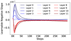
(a) Layerwise learnable slope

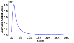
(b) Global learnable slope

Figure 3: Learnable negative slope for leaky ReLU in the FFN of LN-free GPT-2. (a) Layerwise slopes and (b) global slope, both converge toward zero during training, indicating a preference for zero negative slope in LN-free architectures.

To further strengthen our findings, we conducted experiments with a learnable negative slope in the leaky ReLU activation function with two configurations: 1) layer-wise, where each layer has its independent learnable slope, and 2) global, where a single learnable slope is shared across all layers. Results are shown in Figure 3. Interestingly, in the layerwise setting, the early layers initially learn a positive slope while the deeper layers learn a negative slope. However, as training progresses, all layers converge to a near-zero slope. In the global setting, the slope first shifts to positive before converging to near zero. Refer to Figure 12 for their layerwise entropy dynamics.

This highlights the distinct learning dynamics of nonlinearity choices, and a natural preference for zero negative slope, similar to ReLU, in the FFN activation function of the LN-free model.

Observation 2: Early layers in the LayerNorm-Free model with GELU in FFN experience entropic overload. To understand the zero negative slope preference for the FFN activation function in LN-free architecture, we analyzed the headwise entropy values of LN-free models with GELU and ReLU, when trained from scratch, and compared them to their baseline counterparts. Our analysis revealed a significant divergence in the headwise entropy distributions of the LN-free GELU model (see Figure 4). While baseline models with GELU and ReLU exhibit a balanced entropy distribution, by avoiding the extreme values, the LN-free GELU model shows entropic overload in early layers.

Specifically, 58% of heads in the LN-free GELU model have entropy values between $\frac{\text{3max}}{4}$ and ${\tt max}$, compared to only 23% in the LN-free ReLU model (Figure 2ba). More importantly, very few heads in the latter approach maximum entropy compared to the former (see yellow regions in Figure 4c), indicating more severe entropic overload in the LN-free model with GELU.

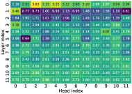
(a) SM + LN + G

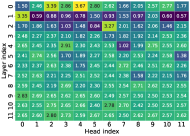
(b) SM + LN + R

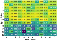
(c) SM + G

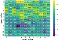
(d) SM + R

Figure 4: Entropy heatmaps of attention for baseline GPT-2 models with GELU and ReLU in the FFN (a and b), compared to their LayerNorm-free counterparts (c and d). In the absence of LayerNorm, using GELU in the FFN results in significantly higher entropic overload than using ReLU.

These observations align with the geometrical properties of ReLUs: they preserve more information about the structure of the raw input, encouraging neurons to specialize in different regions of the input space, leading to a higher intra-class selectivity and specialization (Alleman et al., 2024). Thus, the lack of LayerNorm makes the geometry and specialization effects of ReLU more beneficial.

3.2 Approaches to Prevent Training Collapse in Softmax-Only LLMs

Now, we eliminate the ReLU layer in FFN of LN-free design, resulting in a Softmax-only architecture where FFN is fully linear, and the softmax operation becomes the only source of nonlinearity in the model. We outline the key challenges in training this model and explore their potential solutions.

Observation 3: The softmax-only model exhibits severe entropic overload in the early layers and entropy collapse in the deeper layers. When we train the softmax-only model from scratch, the loss values quickly reach NaN and training collapses. Analyzing the layer-by-layer activation values reveals that activations of the last few layers reach NaN very early in the training phase (Figure 5a). Further investigation into headwise entropy distribution shows that the early layers experience severe entropic overload (Figure 5b), as most of the heads in these layers are stuck at maximum entropy levels (the yellow regions). Conversely, the deeper layers suffer from entropy collapse, characterized by very low entropy values (the blue regions).

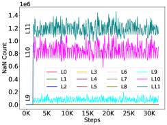
(a) Layerwise NaNs

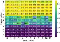
(b) Entropy heatmap

Figure 5: Training collapses in softmax-only GPT-2 model.

Quantitatively, 45% of total heads have entropy values in the range of $\frac{3\text{max}}{4}$ to ${\tt max}$, with most close to the maximum value (Figure 2ba), indicating severe entropic overload. Whereas, 33% of heads exhibit values in the entropy range of 0 to $\frac{\text{max}}{4}$, with most close to zero, indicating entropy collapse, a known indicator of training instability in transformer-based models (Zhai et al., 2023; He et al., 2024).

Observation 4: Normalizing the weights in FFN linear layers or appropriately scaling FFN outputs effectively prevents training collapse in softmax-only models. To prevent training collapse while maintaining PI efficiency, we shift from activation normalization to weight normalization techniques that avoid nonlinear computations at inference. While LayerNorm requires expensive inverse-square-root operations during inference, weight normalization (Salimans & Kingma, 2016) and spectral normalization (Miyato et al., 2018) offer static alternatives. These normalization methods, normalize the weights rather than the activations, incurring no additional cost at inference.

Weight normalization reparameterizes the weight vectors as $\mathbf{W}_{\text{normalized}}=\frac{\mathbf{V}}{\|\mathbf{V}\|_{2}}g$, where $\mathbf{V}$ is reparameterized weight vector, $\|\mathbf{V}\|_{2}$ is Euclidean norm and $g$ is a learnable scaling factor. Whereas, spectral normalization normalizes the weight matrix $\mathbf{W}$ by its largest singular value $\sigma(\mathbf{W})$, yielding $\mathbf{W}_{\text{normalized}}=\frac{\mathbf{W}}{\sigma(\mathbf{W})}$. The former uses the Euclidean norm to control the magnitude of the weights during the training while the latter uses the largest singular value to constrain the Lipschitz constant of the linear layers. We employed these normalizations in the FFN of the softmax-only model which transform $\text{FFN}^{\text{SM}}(\mathbf{X})=(\mathbf{X}\mathbf{W}_{\text{in}}^{\text{ffn}})\mathbf{W}_{\text{out}}^{\text{ffn}}$ as follows:

$$\text{FFN}_{\text{WNorm}}^{\text{SM}}(\mathbf{X})=\left(\mathbf{X}\frac{\mathbf{V}_{\text{in}}^{\text{ffn}}}{\|\mathbf{V}_{\text{in}}\|_{2}}g_{\text{in}}\right)\frac{\mathbf{V}_{\text{out}}^{\text{ffn}}}{\|\mathbf{V}_{\text{out}}\|_{2}}g_{\text{out}}\;\text{and}\;\text{FFN}_{\text{SNorm}}^{\text{SM}}(\mathbf{X})=\left(\mathbf{X}\frac{\mathbf{W}_{\text{in}}^{\text{ffn}}}{\sigma(\mathbf{W}_{\text{in}}^{\text{ffn}})}\right)\frac{\mathbf{W}_{\text{out}}^{\text{ffn}}}{\sigma(\mathbf{W}_{\text{out}}^{\text{ffn}})}$$ (5)

Furthermore, we employ a simpler technique to scale the outputs of the FFN sub-block by having learnable scaling factors for the FFN output and their residual output as follows (see Eq. 1):

$$\mathbf{X}_{\text{out}}=\beta\hat{\mathbf{X}}_{\text{SA}}+\frac{1}{\alpha}(\text{FFN}^{\text{SM}}(\mathbf{X}_{\text{SA}}))\quad\text{where}\quad\alpha,\beta\in\mathbb{R}^{L}$$ (6)

	WNorm	SNorm	Scaled
Eval PPL	3.640	3.624	3.478

Table 2: Perplexity comparison of weight normalization, spectral normalization, and learnable scaling employed in FFN of softmax-only GPT-2 model.

Figure 6 demonstrates the effectiveness of these normalization techniques in stabilizing the training of softmax-only GPT-2 models by preventing entropy collapse in deeper layers. When comparing performance, we find that weight and spectral normalization led to similar performance while the learnable scaling method outperformed them with a lower perplexity (Table 2).

Note that the efficacy of weight or spectral normalization hinges on selecting the appropriate linear layers, as applying them to the linear layers in attention sub-block diminishes overall performance (see Table 8). Refer to Appendix D.1 to understand the effectiveness of the learnable scaling method.

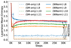
(a) Weight normalization in FFN

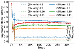
(b) Spectral normalization in FFN

(c) Learnable scaling of FFN outputs

Figure 6: Mitigating entropy collapse in the deeper layers of a softmax-only GPT-2 model by employing weight or spectral normalization in FFN, or by appropriately scaling FFN block outputs.

4 AERO

We propose an AERO framework that tailors the existing LLM architecture by removing nonlinearity and reducing FLOPs count through targeted architectural refinements. Further, we introduce our entropy regularization technique to improve the performance of the Softmax-only model.

4.1 Designing Softmax-only Architecture

To eliminate nonlinearities in existing LLM architectures, we first remove normalization layers, creating an LN-free design. Our approach extends previous work on LN-free design (He et al., 2023; Noci et al., 2023; He & Hofmann, 2024) by also carefully selecting FFN activation functions, opting for ReLU due to its superior PI efficiency and ability to mitigate entropic overload in LN-free models.

We then remove ReLU, leading to a full normalization and activation-free, or Softmax-only, architecture. Training this architecture, however, poses challenges, such as entropy collapse in deeper layers. To address this, we introduce learnable scaling factors, $\alpha$ and $\beta$, in the FFN sub-block, which stabilize training more effectively than weight or spectral normalization.

4.2 FLOPs Reduction in Softmax-only Architecture

To develop an effective FLOPs reduction strategy, we begin by analyzing the distribution of FLOPs between the attention and FFN sub-blocks across varying context lengths.

FFN FLOPs dominates in shorter context length regimes ($T<\frac{8}{3}d$). While prior work on LN-free architectures (He & Hofmann, 2024) has emphasized reducing attention FLOPs, we find that the network’s FLOPs are dominated by FFN FLOPs during inference with shorter context lengths (when $T<\frac{8}{3}d$, Eq. E). For instance, when $T\leq$1K, FFN FLOPs constitute 60%-65% of the total FLOPs in models like GPT-2 (Figure 19) and Pythia (Figure 20) variants.

Given that current research on 2PC PI primarily focuses on smaller context lengths (Zhang et al., 2025; Lu et al., 2025; Zimerman et al., 2024; Pang et al., 2024; Gupta et al., 2024; Hou et al., 2023), we strategically target reducing FFN FLOPs. First, we merge the two linear layers in FFN of Softmax-only architecture—$\mathbf{W}^{\text{ffn}}_{\text{in}}\in\mathbb{R}^{d\times 4d}$ and $\mathbf{W}^{\text{ffn}}_{\text{out}}\in\mathbb{R}^{4d\times d}$—into a single linear layer, $\mathbf{W}^{\text{ffn}}\in\mathbb{R}^{d\times d}$, as they effectively perform linear transformation in the absence of intervening nonlinearity. This reduces FFN FLOPs by a 8$\times$ without any performance degradation, which is not achievable in polynomial transformers, where GELU is approximated by polynomials (Zimerman et al., 2024; Li et al., 2023a).

To reduce FFN FLOPs even further, we ask the following questions: What functional role do FFNs serve when they are purely linear? Do all FFNs contribute equally, or can some of them be pruned?

Figure 7: Overview of the proposed AERO method for reducing nonlinearities and FLOPs in transformer-based LLMs for efficient PI. The bottom of the figure shows the evolution of entropy in the attention mechanism and its distribution across attention heads.

Early FFNs in Softmax-only architecture are critical, while deeper ones can be pruned. We observe that early FFNs, despite being purely linear, are crucial for training stability, as their removal leads to entropy collapses (Fig. 15 and Fig. 16). Deeper FFNs, however, exhibit redundancy, allowing additional FLOPs reduction without degrading performance. This observation resonates with findings on the significance of early-to-mid (conventional non-linear) FFNs (Nanda et al., 2023; Sharma et al., 2024; Jin et al., 2024; Hu et al., 2024; Stolfo et al., 2023; Wang et al., 2023; Haviv et al., 2023; Meng et al., 2022) and the redundant FFN computations (Kobayashi et al., 2024; Pires et al., 2023).

This enables an additional opportunity to reduce FFN FLOPs by selectively removing deeper FFNs. In Softmax-only GPT-2-small architecture, we successfully remove up to six deeper FFNs, achieving an additional 6$\times$ FLOPs reduction in FFN. We refer to this simplified model as ${\tt SM+ScFuFFNi_{x}}$, where $x$ represents the number of deeper FFNs that are replaced with identity functions, while the remaining FFNs have one (fused) linear layer. When $x$=0, we represent the model as ${\tt SM+ScFuFFN}$.

4.3 Entropy Regularization

Challenges in designing entropy regularization schemes to prevent entropic overload. Previous entropy regularization approaches have primarily aimed at penalizing low-entropy predictions (Setlur et al., 2022; Pereyra et al., 2017), based on the principle of maximum entropy (Jaynes, 1982). Recently, (He et al., 2024) introduced entropy regularization to prevent entropy collapses, by addressing extremely low entropy values, in LLMs.

However, our goal is to regularize higher entropy values, which presents two-fold challenges: (1) Head specialization: Since each attention head captures different aspects of the input, the regularization strength needs to be adjusted for each head individually. (2) Preventing over-regularization: Some heads naturally exhibit higher entropy even in well-behaved entropy distributions, thus, penalizing all high-entropy values without distinction could be harmful, requiring a more flexible approach.

Key design principles for entropy regularization. Followings are the key design principles for our entropy regularization scheme (see Algorithm 1), addressing the aforementioned challenges:

• Balanced entropy distribution with parameterized attention matrix: Inspired by Miller et al. (1996), which used temperature parameter as a Lagrangian multiplier to control the entropy of a stochastic system, we parameterized the attention matrix by a learnable temperature $t\in\mathbb{R}^{H\times T}$ for each softmax operation, allowing the model to adjust the sharpness of the attention scores (see Appendix A.3). A higher temperature value ($t>1$) diffuses the attention scores and increases the entropy, while a lower temperature value ($t<1$) sharpens the attention scores and reduces the entropy.

• Dynamic thresholds with head-specific adaptation: To adapt the regularization strength based on the characteristics of each attention head (Voita et al., 2019), we use headwise learnable threshold parameter $\mathtt{reg\_threshold\_weights}\in\mathbb{R}^{H}$. Consequently, the threshold for each head is computed as a learnable fraction of the maximum value of entropy ($\mathtt{reg\_threshold\_weights}\times\text{E}_{\text{max}}$), providing the fine-grained control (see Algorithm 1, line #11).

• Tolerance margin to prevent over-regularization: To prevent over-regularization, we allow small deviations from the respective thresholds. Thus, a penalty is imposed only if the deviation from the threshold exceeds the tolerance margin, which is set as a fraction of $\text{E}_{\text{max}}$ using the hyper-parameter $\gamma$ (see Algorithm1, line #3).

  $$\text{penalty}^{(l,h)}=\begin{cases}\Big{(}\text{deviation}^{(l,h)}\Big{)}^{2}&\text{if }\big{|}\text{deviation}^{(l,h)}\big{|}>\gamma E_{\text{max}}\\ 0&\text{otherwise}\end{cases}$$

  The deviation from threshold is computed as $\text{deviation}^{(l,h)}=\text{E}^{(l,h)}(t)-\theta^{(l,h)}\text{E}_{\text{max}}$, where $\theta^{(l,h)}$ is $\mathtt{reg\_threshold\_weights}$. The hyper-parameter $\gamma$ ensures that the model is not excessively penalized for minor deviations from the desired entropy threshold, which could impede its capacity to learn effectively. This careful calibration between stringent regularization and desired flexibility improves the model’s robustness while maintaining its adaptability to various input distributions.

• Maximum entropy reference: We set $E_{\text{max}}=\log(T)$ as a reference point for computing thresholds and tolerance margins to ensure consistency across different layers and heads for regularization. Additionally, it enhances interpretability by providing a quantifiable reference for measuring deviations in entropy, making the regularization process more understandable.

4.4 Putting it All Together

We developed the AERO framework (Figure 7) to systematically eliminate non-linearities and reduce FFN FLOPs from the existing transformer-based LLMs. Given an input baseline LLM, the first two steps, Step1 and Step2, attempt to address the overheads associated with non-linear operations in PI, resulting in a softmax-only architecture. The next step, Step3, aims at reducing FFN FLOPs by fusing the adjacent linear layers, and then selectively pruning deeper FFNs by replacing them with identity functions, resulting in a substantial reduction in FLOPs without destabilizing the model.

Further, to mitigate the entropic overload, and improve the utilization of attention heads, Step4 introduces entropy regularization, keeping the balanced attention distributions by penalizing extreme entropy values. This step plays a crucial role in boosting the performance of the softmax-only model.

5 Results

We conducted experiments with GPT-2 (12 and 18 layers) and Pythia-70M models on the CodeParrot and Languini book datasets, which are standard benchmarks for LLMs (He & Hofmann, 2024; He et al., 2024). Detailed experimental setup can be found in Appendix C.

Entropy regularization prevents entropic overload in Softmax-only models

Figure 8: While normalizing weights or scaling outputs in the FFN of Softmax-only (GPT-2) model prevents entropy collapse, our proposed entropy regularization effectively mitigates entropic overload.

While both weight and spectral normalization, and scaling methods effectively prevent entropy collapse in the deeper layers and stabilize the training of Softmax-only models, they fail to address the issue of entropic overload, (see Figure 8). In contrast, the entropy regularization scheme penalizes the model to avoid extreme entropy values during training, resulting in a more balanced distribution. As a result, it complements the training stabilizing methods by further mitigating entropic overload in the early layers (see Figure 13), improving the utilization of attention heads and leading to improved performance, as demonstrated by lower perplexity.

Comparison of AERO vs SOTA. We apply AERO to GPT-2, with results for each step shown in Figure 1 and a detailed analysis in Table 3. Our approach achieves up to a 4$\times$ reduction in communication overhead and a 1.94$\times$ speedup in end-to-end PI latency.

We also applied AERO optimizations to the LayerNorm-free design proposed in (He & Hofmann, 2024), referred to as SOTA, as they preserve model performance in their normalization-free architecture. While SOTA saves additional attention FLOPs, by introducing one extra LayerNorm layer, compared to AERO, it offers a slight speedup at the cost of significantly worse model performance, as indicated by higher perplexity. Similar observations hold for the Pythia-70M model (see Figure 14).

In terms of scalability, AERO efficiently scales to deeper models (see Table 5) and larger context lengths (see Table 4 and Table 6), whereas SOTA often suffers from training instability under these conditions. Since the contribution of MHA to the model’s pre-training performance becomes more critical in the absence of FFN operations (Lu et al., 2024), we suspect that the aggressive optimization of attention FLOPs in SOTA, unlike AERO, results in inferior performance and training instability.

Significance of learnable thresholds in entropy regularization Figure 9 depicts the learnable threshold parameters ($\mathtt{reg\_threshold\_weights}$) applied in the entropy regularization scheme after the model has been fully trained from scratch. They exhibit significant variability, both across layers and within individual heads of each layers, which reflects the model’s ability to dynamically adjust the regularization strength in response to the specific roles of different attention heads. Such flexibility is essential for tailoring the regularization process to the distinct requirements of each head.

Table 3: Results, and comparison against SOTA (He & Hofmann, 2024), when GPT-2 ($L$=12, $H$=12, $d$=768) model is trained from scratch on CodeParrot (Face, ) dataset with context length 128.

	Network Arch.	PPL	#Nonlinear Ops	#FLOPs		Comm. (GB)	Lat. (min.)	Savings
				FFN	Attn.			Comm.	Lat.
Baseline	${\tt SM+LN+G}$	2.69	SM:$144\times\mathbb{R}^{128\times 128}$	14.5B	7.7B	25.32	8.21	1$\times$	1$\times$
			LN:$24\times\mathbb{R}^{128\times 768}$
			G:$12\times\mathbb{R}^{128\times 3072}$
	${\tt SM+LN+R}$	2.76	SM:$144\times\mathbb{R}^{128\times 128}$	14.5B	7.7B	9.44	6.06	2.68$\times$	1.35$\times$
			LN:$24\times\mathbb{R}^{128\times 768}$
			R:$12\times\mathbb{R}^{128\times 3072}$
SOTA	${\tt SM+ScFFN}$	4.00	SM:$144\times\mathbb{R}^{128\times 128}$	14.5B	3.9B	6.83	5.31	3.71$\times$	1.55$\times$
			LN: $1\times\mathbb{R}^{128\times 768}$
	${\tt SM+ScFuFFN}$	3.97	SM:$144\times\mathbb{R}^{128\times 128}$	1.8B	3.9B	6.31	4.50	4.00$\times$	1.82$\times$
			LN: $1\times\mathbb{R}^{128\times 768}$
	${\tt SM+ScFuFFNi_{1}}$	4.00	SM:$144\times\mathbb{R}^{128\times 128}$	1.2B	3.9B	6.30	4.44	4.00$\times$	1.85$\times$
			LN: $1\times\mathbb{R}^{128\times 768}$
AERO	${\tt SM+ScFFN}$	3.50	SM:$144\times\mathbb{R}^{128\times 128}$	14.5B	7.7B	6.95	5.68	3.64$\times$	1.45$\times$
	${\tt SM+ScFuFFN}$	3.48	SM:$144\times\mathbb{R}^{128\times 128}$	1.8B	7.7B	6.43	4.76	3.94$\times$	1.72$\times$
	${\tt SM+ScFuFFNi_{6}}$	3.54	SM:$144\times\mathbb{R}^{128\times 128}$	0.9B	7.7B	6.29	4.23	4.00$\times$	1.94$\times$
	$\text{EReg}({\tt SM(t)+ScFuFFN})$	3.21	SM:$144\times\mathbb{R}^{128\times 128}$	1.8B	7.7B	6.43	4.76	3.94$\times$	1.72$\times$
	$\text{EReg}({\tt SM(t)+ScFuFFNi_{6}})$	3.25	SM:$144\times\mathbb{R}^{128\times 128}$	0.9B	7.7B	6.29	4.23	4.00$\times$	1.94$\times$

(a) Values of learned threshold weights

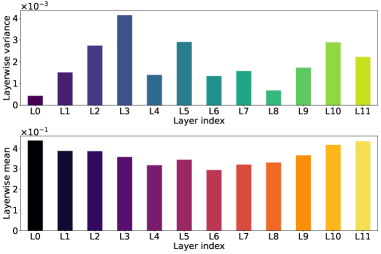
(b) Layerwise mean and variance of threshold weights

Figure 9: Analysis of learned threshold weights ($\mathtt{reg\_threshold\_weights}$, see Eq. • ‣ 4.3) in entropy regularization for softmax-only GPT-2 model: (a) Attention heads adaptively learn non-uniform threshold weights across different heads, setting individualized thresholds for entropy regularization; (b) The non-uniform means and non-zero variances across layers highlight the necessity and effectiveness of headwise learnable thresholds in adapting regularization strength.

6 Conclusion

In this work, we introduce AERO, a four-stage design framework to streamline the existing LLM architecture for efficient private inference. We design Softmax-only architecture with significantly lower FLOPs and propose entropy regularization to boost their performance.

Limitations. This study mainly focuses on pre-training performance, with perplexity as the primary metric, and does not include experiments to evaluate other capabilities such as transfer learning or few-shot learning. Additionally, the efficacy of the proposed Softmax-only models has been validated on models with fewer than 1B parameters. Future work will explore broader experimental evaluations, including the adaption of AERO for large-scale models (see Appendix H).

Appendix

Appendix A Shannon Entropy and Its Application in Transformer LLMs

A.1 Why Use Entropy to Evaluate the Impact of Nonlinearities?

We use entropy as a metric to study the impact of nonlinearities on the transformer-based LLMs for the following reasons:

• Quantifying attention distribution: The attention mechanism lies at the core of transformer architectures, and by computing the entropy of attention score distributions, we can observe how nonlinearities influence the spread (or the concentration) of attention scores. Higher entropy implies a more exploratory behavior, while lower entropy suggests a more focused attention distribution.

• Feature selection: Nonlinearities, such as ReLU, enhance feature selectivity by amplifying important features and suppressing less relevant ones (Alleman et al., 2024; Maas et al., 2013). Entropy can measure this selectivity across layers and heads, providing insights into the model’s prioritization of information. Previous studies have used entropy to capture layer-wise information flow in neural networks (Peer et al., 2022).

• Exploration vs. exploitation: Nonlinear operators like the self-attention mechanism, LayerNorm, and GELU balance exploration and exploitation by selecting relevant features while considering a broader context. For instance, heads in the first layer focus on exploration, while those in the second layer focus on exploitation. (see Figures 4a, 4b, 11a and 11b).

• Systematic assessment: Prior work Zhang et al. (2024); Nahshan et al. (2024); Zhai et al. (2023); Vig & Belinkov (2019); Ghader & Monz (2017) also used entropy to analyze the behavior of transformer-based models; thus, enhancing validity and comparability of our findings.

A.2 Evaluating the Sharpness of Attention Score Distributions Using Entropy

Shannon’s entropy quantifies the uncertainty in a probability distribution, measuring the amount of information needed to describe the state of a stochastic system (Shannon, 1948; Jaynes, 1957). For a probability distribution $P(x)$, the entropy is defined as $\mathbf{E}(P)=-\sum_{i}P(x_{i})\log P(x_{i})$. Refer to (Baez, 2024) for details on entropy.

In a softmax-based attention mechanism, each softmax operation yields an entropy value representing the sharpness or spread of the attention scores for each query position (Ghader & Monz, 2017; Vig & Belinkov, 2019). Higher entropy indicates a more uniform distribution of softmax scores, while lower entropy signifies a more focused distribution on certain features (Nahshan et al., 2024).

Let $\mathbf{A}^{(h,l)}\in\mathbb{R}^{T\times T}$ be the attention matrix of $h$-th head in $l$-th layer, and each element in the attention matrix, $a_{ij}^{(l,h)}$, are attention weights for the $i$-th query and $j$-th key, which are non-negative and sum to one for a query:

$$\mathbf{A}^{(l,h)}=\left[a_{ij}^{(l,h)}\right]_{T\times T},\quad\text{where}\quad a_{ij}^{(l,h)}\geq 0\quad\text{and}\quad\sum_{j=1}^{T}a_{ij}^{(l,h)}=1$$ (7)

This square matrix is generated by applying the softmax operation over the key length for each query position as follows (i.e., $\mathbf{X}\in\mathbb{R}^{T\times T}$ $\mathbf{X}_{i}\in\mathbb{R}^{1\times T}$ ):

$$\mathbf{A}^{(h,l)}(\mathbf{X})=\text{Softmax}\Big{(}\frac{1}{\sqrt{d_{k}}}(\mathbf{X}\mathbf{W}^{Q})(\mathbf{X}{\mathbf{W}^{K}})^{\top}\Big{)},\;\text{where}\quad\text{Softmax}(\mathbf{X}_{i})=\frac{\exp\left(x_{i}\right)}{\sum_{j=1}^{T}\exp\left(x_{j}\right)}$$ (8)

Thus, each element $a_{ij}^{(l,h)}$ of the attention matrix can be represented as follows:

$$a_{ij}^{(l,h)}=\frac{\exp\left(\frac{1}{\sqrt{d_{k}}}(\mathbf{X}_{i}\mathbf{W}^{Q})(\mathbf{X}_{j}\mathbf{W}^{K})^{\top}\right)}{\sum_{k=1}^{T}\exp\left(\frac{1}{\sqrt{d_{k}}}(\mathbf{X}_{i}\mathbf{W}^{Q})(\mathbf{X}_{k}\mathbf{W}^{K})^{\top}\right).}$$ (9)

Following (Zhai et al., 2023), we compute the mean of entropy values across all query positions to obtain a single entropy value for each head. The entropy $\mathbf{E}^{(l,h)}$ for the $h$-th head in the $l$-th layer of an attention matrix is given by:

$$\mathbf{E}^{(l,h)}=-\frac{1}{T}\sum_{i=1}^{T}\sum_{j=1}^{T}a_{ij}^{(l,h)}\log\left(a_{ij}^{(l,h)}+\epsilon\right)$$ (10)

where $\epsilon$ is a small constant added for numerical stability to prevent taking the log of zero.

A.3 Relationship Between Temperature and Shannon Entropy

With the learnable temperature parameters ($t$), the attention matrix can be expressed as follows:

$$\mathbf{A}^{(l,h)}(t)=\left[a_{ij}^{(l,h)}(t)\right]_{T\times T},\;\text{where}\;a_{ij}^{(l,h)}(t)=\frac{\exp\left(\frac{1}{t_{i}\sqrt{d_{k}}}(\mathbf{X}_{i}\mathbf{W}^{Q})(\mathbf{X}_{j}\mathbf{W}^{K})^{\top}\right)}{\sum_{k=1}^{T}\exp\left(\frac{1}{t_{i}\sqrt{d_{k}}}(\mathbf{X}_{i}\mathbf{W}^{Q})(\mathbf{X}_{k}\mathbf{W}^{K})^{\top}\right).}$$ (11)

Let $z_{ij}=\left(\mathbf{X}_{i}\mathbf{W}^{Q}\right)\left(\mathbf{X}_{j}\mathbf{W}^{K}\right)^{\top}$ represents the logits (attention scores before applying softmax).

Now, substituting $a_{ij}^{(l,h)}(t)$ into the entropy formula:

$$\mathbf{E}^{(l,h)}(t)=-\frac{1}{T}\sum_{i=1}^{T}\sum_{j=1}^{T}\frac{\exp\left(\frac{1}{t\sqrt{d_{k}}}z_{ij}\right)}{\sum_{k=1}^{T}\exp\left(\frac{1}{t\sqrt{d_{k}}}z_{ik}\right)}\log\left(\frac{\exp\left(\frac{1}{t\sqrt{d_{k}}}z_{ij}\right)}{\sum_{k=1}^{T}\exp\left(\frac{1}{t\sqrt{d_{k}}}z_{ik}\right)}\right).$$

Simplifying the logarithmic term:

$$\log\left(\frac{\exp\left(\frac{1}{t\sqrt{d_{k}}}z_{ij}\right)}{\sum_{k=1}^{T}\exp\left(\frac{1}{t\sqrt{d_{k}}}z_{ik}\right)}\right)=\frac{1}{t\sqrt{d_{k}}}z_{ij}-\log\left(\sum_{k=1}^{T}\exp\left(\frac{1}{t\sqrt{d_{k}}}z_{ik}\right)\right).$$

Thus, the entropy simplifies to:

$$\mathbf{E}^{(l,h)}(t)=\frac{1}{T}\sum_{i=1}^{T}\left(\log\left(\sum_{k=1}^{T}\exp\left(\frac{1}{t\sqrt{d_{k}}}z_{ik}\right)\right)-\frac{1}{t\sqrt{d_{k}}}\sum_{j=1}^{T}a_{ij}^{(l,h)}(t)z_{ij}\right).$$

Further, it can be simplified as a function of expected value of $z_{ij}$ under the attention distribution:

$$\mathbf{E}^{(l,h)}(t)=\frac{1}{T}\sum_{i=1}^{T}\left(\log\left(\sum_{k=1}^{T}\exp\left(\frac{z_{ik}}{t\sqrt{d_{k}}}\right)\right)-\frac{1}{t\sqrt{d_{k}}}\,\mathbb{E}_{j\sim a_{ij}^{(l,h)}(t)}[\,z_{ij}\,]\right)$$ (12)

In the above expression (Eq. 12), the first term $\left(\log\sum\right)$ represents the overall spread of the logits when scaled by $t$, and the second term $\left(\frac{1}{t}\mathbb{E}[z_{ij}]\right)$ represents the expected value of the scaled logits under the attention distribution.

Temperature cases when:

1. $t>1$: The scaling factor $\frac{1}{t}$ reduces the influence of the logits $z_{ij}$, making the softmax distribution more uniform. Consequently, the entropy increases.

2. $t<1$: The scaling factor $\frac{1}{t}$ increases the influence of the logits $z_{ij}$, making the softmax distribution more peaked. Consequently, the entropy decreases.

3. $t\to\infty$: The logits are scaled down to zero, and the softmax becomes a uniform distribution. The entropy reaches its maximum value of $\log T$.

4. $t\to 0$: The logits dominate the softmax, and it becomes a one-hot distribution. The entropy approaches zero.

Appendix B Integrations of Entropy Regularization in Loss Function

B.1 Entropy Regularization Algorithm

Algorithm 1 Entropy Regularization Loss Computation

Inputs: attentions: List of attention matrices, $\Theta(L,H)$= reg_threshold_weights, $T$: Sequence length, $\lambda$: Regularization loss weightage, $\gamma$: Hyper-parameter for Tolerance margin
Output: $\mathcal{L}_{\text{total}}$: Total loss including entropy regularization

1:$\mathcal{L}_{\text{entropy}}\leftarrow 0$

2:$\text{E}_{\text{max}}\leftarrow\log(T)$ $\triangleright$ Theoretical maximum value of entropy

3:$\text{Tol}_{\text{margin}}\leftarrow\gamma\text{E}_{\text{max}}$ $\triangleright$ Tolerance margin is set as a small fraction of $\text{E}_{\text{max}}$

4:for each layer $l$ in layers do

5:     $\mathcal{L}_{\text{layer}}\leftarrow 0$

6:     $\text{A}(t)\leftarrow\text{attentions}[l]$ $\triangleright$ Attention matrix with learnable temperature for each query position

7:     $\text{E}(t)\leftarrow-\frac{1}{T}\sum_{i=1}^{T}\sum_{j=1}^{T}\text{A}_{ij}(t)\log(\text{A}_{ij}(t))$ $\triangleright$ Compute entropy, averaged over query length

8:     for each head $h$ in heads do

9:         $E^{(l,h)}\leftarrow\text{Slice}(\text{E}(t),h)$ $\triangleright$ Entropy for head $h$

10:         $\theta^{(l,h)}\leftarrow\text{Slice}(\Theta{(L,H),h})$ $\triangleright$ Learnable threshold weight head $h$

11:         $\delta^{(l,h)}\leftarrow\text{E}^{(l,h)}(t)-\theta^{(l,h)}\text{E}_{\text{max}}$ $\triangleright$ Deviation from head-specific threshold

12:         $\text{penalty}^{(l,h)}\leftarrow(\delta^{(l,h)})^{2}\mathds{1}(|\delta^{(l,h)}|>\text{Tol}_{\text{margin}})$ $\triangleright$ Penalize iff deviation exceeds Tolerance

13:         $\mathcal{L}_{\text{layer}}\leftarrow\mathcal{L}_{\text{layer}}+\text{penalty}^{(l,h)}$

14:     end for

15:     $\mathcal{L}_{\text{layer}}\leftarrow\frac{\mathcal{L}_{\text{layer}}}{\text{num\_heads}}$ $\triangleright$ Average over heads

16:     $\mathcal{L}_{\text{entropy}}\leftarrow\mathcal{L}_{\text{entropy}}+\mathcal{L}_{\text{layer}}$

17:end for

18:$\mathcal{L}_{\text{entropy}}\leftarrow\frac{\mathcal{L}_{\text{entropy}}}{\text{len(attentions)}}$ $\triangleright$ Average over layers

19:$\mathcal{L}_{\text{total}}\leftarrow\mathcal{L}_{\text{CE}}+\lambda\mathcal{L}_{\text{entropy}}$

20:return $\mathcal{L}_{\text{total}}$

B.2 PyTorch Implementation of Entropy Regularization

The PyTorch implementation below computes the entropy regularization loss for attention weights in a transformer model. This regularization ensures a balanced attention distribution, preventing it from becoming overly concentrated or too diffuse.

PyTorch Implementation 1: Entropy Regularization Loss Calculation

⬇

1import torch

2

3def calculate_entropy_reg_loss(attentions, blocks, seq_len):

4 """

5 Calculate the entropy regularization loss.

6

7 Parameters:

8 attentions (list): A list of attention matrices from different layers.

9 blocks (list): A list of transformer blocks.

10 seq_len (int): The length of the sequence (context length).

11

12 Returns:

13 float: The entropy regularization loss.

14 """

15 entropy_reg_loss = 0

16 max_entropy = torch.log(torch.tensor(seq_len)) # Theoretical maximum entropy

17 fraction = 0.10 # Design hyper-parameter for tolerance margin

18 tolerance_margin = fraction * max_entropy # Set tolerance margin as fraction of the maximum entropy

19

20 for layer_idx, (block, attn_mat) in enumerate(zip(blocks, attentions)):

21 reg_threshold_weights = block.attn.reg_threshold_weights # Head-wise learnable parameters to set head-specific threshold

22 ent_val = -torch.sum(attn_mat * torch.log(attn_mat + 1e-9), dim=-1) # Compute entropy averaged over sequence length

23 layer_entropy_reg_loss = 0

24

25 for head_idx in range(block.attn.num_heads):

26 head_entropy = ent_val[:, head_idx, :] # Get head-specific entropy

27 threshold = reg_threshold_weights[head_idx] * max_entropy

28 deviation = torch.abs(head_entropy - threshold)

29 penalty = torch.square(torch.where(deviation > tolerance_margin, deviation, torch.zeros_like(deviation)))

30 layer_entropy_reg_loss += penalty.sum()

31

32 layer_entropy_reg_loss /= block.attn.num_heads

33 entropy_reg_loss += layer_entropy_reg_loss

34

35 entropy_reg_loss /= len(attentions)

36 return entropy_reg_loss

37

38# Calculate the total loss including entropy regularization

39lambda_reg = 1e-5 # Hyperparameter for entropy regularization weight

40entropy_regularization = calculate_entropy_reg_loss(attentions, blocks, seq_len)

41total_loss = ce_loss + lambda_reg * entropy_regularization

Appendix C Design of Experiments

System setup We use a SecretFlow setup (Lu et al., 2025) with the client and server simulated on two physically separate machines, each equipped with an AMD EPYC 7502 server with specifications of 2.5 GHz, 32 cores, and 256 GB RAM. We measure the end-to-end PI latency, including input embeddings and final output (vocabulary projection) layers, in WAN setting (bandwidth:100Mbps, latency:80ms), simulated using Linux Traffic Control (tc) commands. The number of threads is set to 32. Following He & Hofmann (2024); Stanić et al. (2023); Geiping & Goldstein (2023), all the models are trained on a single RTX 3090 GPU.

Datasets We train models from scratch using the CodeParrot Face and Languini book Stanić et al. (2023) datasets. The CodeParrot dataset, sourced from 20 million Python files on GitHub, contains 8 GB of files with 16.7 million examples, each with 128 tokens, totaling 2.1 billion training tokens. We use a tokenizer with a vocabulary of 50K and train with context lengths of 128 and 256. The Languini book dataset includes 84.5 GB of text from 158,577 books, totaling 23.9 billion tokens with a WikiText-trained vocabulary of 16,384, and train with context length of 512. Each book averages 559 KB of text or about 150K tokens, with a median size of 476 KB or 128K tokens.

Training Hyperparameters For pre-training on the CodeParrot dataset, we adopt the training settings from (He & Hofmann, 2024). Similarly, for training on the Languini dataset, we follow the settings from (Stanić et al., 2023). These settings remain consistent across all architectural variations to accurately reflect the impact of the architectural changes. When applying entropy regularization on the CodeParrot dataset, we initialize the learnable temperature to 1e-2 and set $\lambda$ to 1e-5. For the Languini dataset, the temperature is initialized to 1e-1, and $\lambda$ is set to 5e-5.

C.1 Perplexity as a Reliable Metric to Evaluate the LLMs’ Performance

Perplexity (Jelinek et al., 1977) is a widely adopted metric to evaluate the predictive performance of auto-regressive language models, reflecting the model’s ability to predict the next token in a sequence. However, for perplexity to serve as a meaningful comparative metric across different architectures, it is critical to ensure consistency in the tokenizer, and vocabulary size and quality (Hutchins et al., 2022). Any variation in these components can potentially skew the results by inflating or deflating perplexity scores; thus, obfuscating the true effects of architectural changes.

In our work, we maintain tokenization schemes and vocabulary attributes as invariant factors across all experiments within a dataset. This isolation of architectural modifications ensures that any observed variations in perplexity are directly attributable to changes in the model design. Thus, by enforcing a consistent tokenization scheme and vocabulary within a dataset, we ensure that perplexity remains a reliable metric for comparing model architectures. Consequently, lower perplexity in our evaluations reliably reflects improved token-level predictions.

C.2 Why Training from Scratch to Study Nonlinearities?

Understanding the intricate roles of architectural components and nonlinearities—such as activation functions (e.g., GELU, ReLU) in FFN, normalization layers (e.g., LayerNorm), etc.—in transformer-based language models necessitates a methodical and detailed investigative approach. Training models from scratch is essential for this purpose, as it allows us to delve into the internal mechanisms of the model using quantitative measures like entropy. Below, we present a justification for our methodology:

• Nonlinearities’ impact on the fundamental learning dynamics: Nonlinearities significantly influence the optimization landscape by affecting gradient flow and the model’s ability to navigate non-convex loss surfaces. Training models from scratch allow us to observe the fundamental learning dynamics that emerge during the initial stages of training. Thus, constructing models with controlled variations, such as substituting or excluding specific nonlinearities, enables us to isolate their direct effects impact on convergence behavior and training stability.

• Understanding internal mechanisms through entropy analysis: Training from scratch enables us to navigate the evolution of entropy values across the layers and assess how architectural components influence information flow within the model. This analysis provides deep insights into the internal workings of models that may not be accessible when starting from pre-trained checkpoints.

• Limitations of fine-tuning approaches: The aforementioned granular level of analysis is unattainable when starting from pre-trained models, where the optimization trajectory has already been largely determined. In contrast, training models from scratch eliminates confounding variables that could arise from pre-existing weights and learned representations, ensuring that any observed effects are solely due to the architectural modifications introduced.

Appendix D Additional Results

D.1 Learnable Scaling Factors in Scaled-FFN of Softmax-only Architecture

We plot the values of FFN scaling factors $\alpha$ and $\beta$ (see Eq. 6) learned across the layers in the full-trained softmax-only GPT-2 model, and made the following observations from the Figure 10:

• Significant increase in $\alpha$ with layer depth: The scaling factor $\alpha$ increases substantially in the deeper layers of the model, with particularly high values observed in L10. This indicates that as the network goes deeper, the FFN outputs are heavily scaled down by $\alpha$. This downscaling is essential to prevent the FFN outputs from dominating the activations, which could otherwise lead to numerical instability, as evidenced by the NaNs observed early in training in Figure 5a. The large $\alpha$ values in deeper layers suggest that this downscaling becomes increasingly critical as the model progresses through its layers, effectively stabilizing the training process by keeping the FFN outputs in check.

• Balancing $\beta$ values across layers: The $\beta$ scaling factors, which modulate the residual connections within the FFN sub-block by up-scaling their output, start higher in the earlier layers and gradually decrease, with some fluctuation, as the layers deepen. The moderate up-scaling provided by $\beta$ helps to ensure that the residual connections are not overshadowed by the scaled-down FFN outputs. This balance between the strong downscaling by $\alpha$ and the corresponding upscaling by $\beta$ is crucial for maintaining stable activations across layers, particularly in deeper layers where instability is most likely to occur.

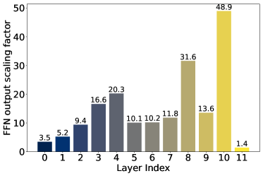
(a) FFN output scaling factor $\alpha$

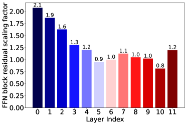
(b) FFN-block’s residual scaling factor $\beta$

Figure 10: Learned scaling factors $\alpha$ and $\beta$ in Eq. 6 across different layers in the Softmax-only GPT-2 model ($L$=12, $H$=12, $d$=768). The values were plotted after full model training to observe the modulation of FFN outputs and residual connections in each layer.

These observations underscore the critical role that the learnable scaling factors $\alpha$ and $\beta$ play in stabilizing the training of softmax-only GPT-2 models. By dynamically adjusting the contributions of the FFN sub-block outputs, $\alpha$ and $\beta$ prevent the numerical issues that arise in deeper layers, ensuring stable and effective training. This fine-tuned balance is key to avoiding entropy collapse and other forms of instability that would otherwise derail the training process.

D.2 Entropy Dynamics in LLM Architecture with Fewer Nonlinearity

Figure 11 presents the entropy dynamics of the GPT-2 model as nonlinearities are progressively removed, with the models trained from scratch. In Figure 12, the entropy dynamics are shown for a normalization-free GPT-2 model with a learnable negative slope in leaky ReLU of FFN. Figure 13 represents the entropy dynamics when various methods of mitigating the training instability (weight and spectral normalization in FFN, and learnable scaling factors for FFN outputs) in Softmax-only GPT-2 modes are applied, and also for entropy-regularization which is applied to overcome the entropic overload.

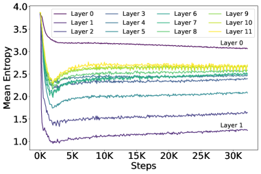
(a) SM + LN + G

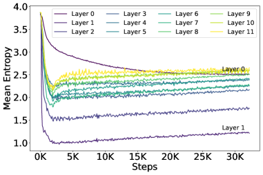
(b) SM + LN + R

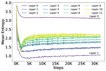
(c) SM + LN

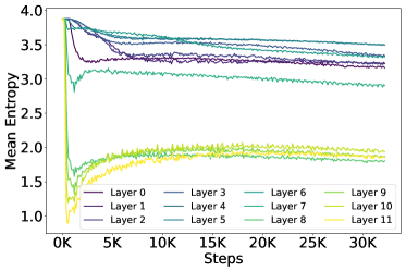
(d) SM + G

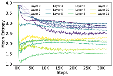
(e) SM + R

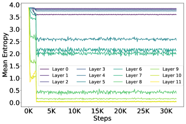
(f) SM

Figure 11: Evolution of Layerwise entropy when GPT-2 ($L$=12, $H$=12, $d$=768) models with various nonlinearity configurations are trained from scratch on CodeParrot dataset.

(a) Layerwise learnable slope

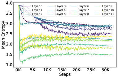
(b) Global slope

Figure 12: Evolution of layerwise entropy in LayerNorm-free GPT-2 models ($L$ = 12, $H$ = 12, $d$ = 768) with a learnable negative slope in the leaky ReLU activation function, trained from scratch on the CodeParrot dataset

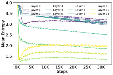
(a) Weight normalization in FFN

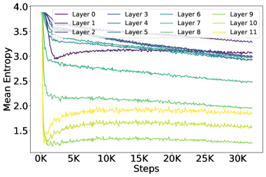
(b) Spectral normalization in FFN

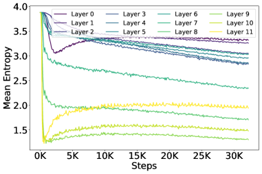
(c) Scaled-FFN

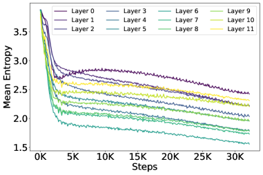
(d) Entropy regularization

Figure 13: "Layerwise entropy evolution in Softmax-only GPT-2 models ($L$ = 12, $H$ = 12, $d$ = 768), trained from scratch on the CodeParrot dataset. Weight and spectral normalization techniques, along with learnable scaling factors (scaled-FFN), are applied in the FFN. In the final configuration (d), entropy regularization is used within the scaled-FFN to address the entropic overload observed in early layers. Notably, the entropy in early layers of (d) is lower compared to (a), (b), and (c).

D.3 Additional Results for Latency and Communication Savings using AERO

GPT-2 Model with 256 tokens as input context Table 4 provides an analysis of the latency and communication savings achieved by applying AERO to the GPT-2 model with 256 context length, along with a detailed breakdown of the nonlinear operations and FLOPs. The performance of AERO is also compared against SOTA.

Table 4: Results, and comparison against SOTA (He & Hofmann, 2024), when GPT-2 ($L$=12, $H$=12, $d$=768) model is trained from scratch on CodeParrot (Face, ) dataset with context length 256. NaNs indicate training instability in SOTA.

	Network Arch.	PPL	#Nonlinear Ops	#FLOPs		Comm. (GB)	Lat. (min.)	Savings
				FFN	Attn.			Comm.	Lat.
Baseline	${\tt SM+LN+G}$	2.35	SM:$144\times\mathbb{R}^{256\times 256}$	29.0B	16.3B	58.51	16.57	1$\times$	1$\times$
			LN:$24\times\mathbb{R}^{256\times 768}$
			G:$12\times\mathbb{R}^{256\times 3072}$
	${\tt SM+LN+R}$	2.41	SM:$144\times\mathbb{R}^{256\times 256}$	29.0B	16.3B	26.73	12.59	2.19$\times$	1.32$\times$
			LN:$24\times\mathbb{R}^{256\times 768}$
			R:$12\times\mathbb{R}^{256\times 3072}$
SOTA	${\tt SM+ScFFN}$	3.47	SM:$144\times\mathbb{R}^{256\times 256}$	29.0B	8.5B	21.52	11.42	2.72$\times$	1.45$\times$
			LN: $1\times\mathbb{R}^{256\times 768}$
	${\tt SM+ScFuFFN}$	NaNs	SM:$144\times\mathbb{R}^{256\times 256}$	3.6B	8.5B	20.48	10.14	2.86$\times$	1.63$\times$
			LN: $1\times\mathbb{R}^{256\times 768}$
AERO	${\tt SM+ScFFN}$	3.04	SM:$144\times\mathbb{R}^{256\times 256}$	29.0B	16.3B	21.77	11.91	2.69$\times$	1.39$\times$
	${\tt SM+ScFuFFN}$	3.03	SM:$144\times\mathbb{R}^{256\times 256}$	3.6B	16.3B	20.72	10.45	2.82$\times$	1.59$\times$
	${\tt SM+ScFuFFNi_{6}}$	3.08	SM:$144\times\mathbb{R}^{256\times 256}$	1.8B	16.3B	20.59	10.32	2.84$\times$	1.61$\times$
	$\text{EReg}({\tt SM(t)+ScFuFFN})$	2.92	SM:$144\times\mathbb{R}^{256\times 256}$	3.6B	16.3B	20.72	10.45	2.82$\times$	1.59$\times$
	$\text{EReg}({\tt SM(t)+ScFuFFNi_{6}})$	2.97	SM:$144\times\mathbb{R}^{256\times 256}$	1.8B	16.3B	20.59	10.32	2.84$\times$	1.61$\times$

GPT-2 Model with 18 Layers Table 5 provides an analysis of the latency and communication savings achieved by applying AERO to the 18-layer GPT-2 model, along with a detailed breakdown of the nonlinear operations and FLOPs. The performance of AERO is also compared against SOTA.

Table 5: Results, and comparison against SOTA (He & Hofmann, 2024), when GPT-2 ($L$=18, $H$=12, $d$=768) model is trained from scratch on CodeParrot (Face, ) dataset with context length 128. NaNs indicate training instability in SOTA.

	Network Arch.	PPL	#Nonlinear Ops	#FLOPs		Comm. (GB)	Lat. (min.)	Savings
				FFN	Attn.			Comm.	Lat.
Baseline	${\tt SM+LN+G}$	2.56	SM:$216\times\mathbb{R}^{128\times 128}$	21.7B	11.6B	37.17	10.77	1$\times$	1$\times$
			LN:$36\times\mathbb{R}^{128\times 768}$
			G:$18\times\mathbb{R}^{128\times 3072}$
	${\tt SM+LN+R}$	2.63	SM:$216\times\mathbb{R}^{128\times 128}$	21.7B	11.6B	13.34	8.04	2.79$\times$	1.34$\times$
			LN:$36\times\mathbb{R}^{128\times 768}$
			R:$18\times\mathbb{R}^{128\times 3072}$
SOTA	${\tt SM+ScFFN}$	NaNs	SM:$216\times\mathbb{R}^{128\times 128}$	21.7B	5.9B	9.39	6.75	3.96$\times$	1.60$\times$
			LN: $1\times\mathbb{R}^{128\times 768}$
AERO	${\tt SM+ScFFN}$	3.26	SM:$216\times\mathbb{R}^{128\times 128}$	21.7B	11.6B	9.62	7.23	3.86$\times$	1.49$\times$
	${\tt SM+ScFuFFN}$	3.24	SM:$216\times\mathbb{R}^{128\times 128}$	2.7B	11.6B	8.83	6.07	4.21$\times$	1.77$\times$
	${\tt SM+ScFuFFNi_{4}}$	3.27	SM:$216\times\mathbb{R}^{128\times 128}$	2.1B	11.6B	8.79	5.85	4.23$\times$	1.84$\times$
	$\text{EReg}({\tt SM(t)+ScFuFFN})$	3.13	SM:$216\times\mathbb{R}^{128\times 128}$	2.7B	11.6B	8.83	6.07	4.21$\times$	1.77$\times$
	$\text{EReg}({\tt SM(t)+ScFuFFNi_{4}})$	3.17	SM:$216\times\mathbb{R}^{128\times 128}$	2.1B	11.6B	8.79	5.85	4.23$\times$	1.84$\times$

D.4 Results on Languini Dataset

Table 6 provides an analysis of the latency and communication savings achieved by applying AERO to the GPT-2 model on Languini dataset, trained on 1.2B, 2.4B, and 4.8B tokens. We also provides a detailed breakdown of the nonlinear operations and FLOPs.

Table 6: Results, and comparison against SOTA (He & Hofmann, 2024), when GPT-2 ($L$=12, $H$=12, $d$=768) model is trained from scratch on Languini (Stanić et al., 2023) dataset with context length 512. NaNs indicate training instability in SOTA.

	Network Arch.	Eval PPL			#Nonlinear Ops	#FLOPs		Comm. (GB)	Lat. (min.)
		1.2B	2.4B	4.8B		FFN	Attn.
Baseline	${\tt SM+LN+G}$	25.71	23.32	21.29	SM:$144\times\mathbb{R}^{512\times 512}$	58.0B	36.2B	145.24	30.74
					LN:$24\times\mathbb{R}^{512\times 768}$
					G:$12\times\mathbb{R}^{512\times 3072}$
	${\tt SM+LN+R}$	26.06	23.55	21.58	SM:$144\times\mathbb{R}^{512\times 512}$	58.0B	36.2B	81.71	23.54
					LN:$24\times\mathbb{R}^{512\times 768}$
					R:$12\times\mathbb{R}^{512\times 3072}$
SOTA	${\tt SM+ScFFN}$	NaNs	NaNs	NaNs	SM:$144\times\mathbb{R}^{512\times 512}$	58.0B	19.3B	72.10	21.56
					LN: $1\times\mathbb{R}^{512\times 768}$
AERO	${\tt SM+ScFFN}$	33.91	31.12	28.89	SM:$144\times\mathbb{R}^{512\times 512}$	58.0B	36.2B	71.76	21.51
	${\tt SM+ScFuFFN}$	33.77	30.82	28.59	SM:$144\times\mathbb{R}^{512\times 512}$	7.3B	36.2B	69.68	19.44
	${\tt SM+ScFuFFNi_{1}}$	34.16	31.23	29.69	SM:$144\times\mathbb{R}^{512\times 512}$	6.6B	36.2B	69.64	19.11
	$\text{EReg}({\tt SM(t)+ScFuFFN})$	31.54	28.70	26.55	SM:$144\times\mathbb{R}^{512\times 512}$	7.3B	36.2B	69.68	19.44
	$\text{EReg}({\tt SM(t)+ScFuFFNi_{1}})$	31.75	28.93	26.74	SM:$144\times\mathbb{R}^{512\times 512}$	6.6B	36.2B	69.64	19.11

D.5 Results on Pythia-70M

Table 7 presents the pre-training performance, measured in terms of perplexity, for input context lengths of 128 and 256. The results show the impact of progressively removing nonlinearities from the Pythia-70M model.

Table 7: Results for nonlinearity reduction in Pythia-70M ($L$=6, $H$=8, $d$=512) on CodeParrot dataset. LN-free architecture with ReLU activations in FFN (i.e., ${\tt SM+R}$) significantly outperform their GELU counterpart (i.e., ${\tt SM+G}$) across various content length ($T$).

	$T$=128		$T$=256
	Eval PPL	+$\Delta$(%)	Eval PPL	+$\Delta$(%)
SM+LN+G	3.512	0.00	3.054	0.00
SM+LN+R	3.590	2.22	3.107	1.73
SM+LN	4.445	26.56	3.836	25.60
SM+G	4.086	16.35	3.570	16.87
SM+R	3.736	6.36	3.273	7.17

Figure 14 illustrates the step-wise latency and communication savings achieved by applying AERO, as well as its impact on perplexity, on Pythia-70M models, also, compares with the SOTA at iso-latencies.

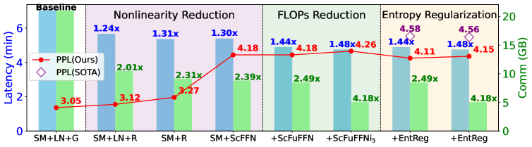
Figure 14: Latency and communication savings through nonlinearity and FLOPs reduction steps when AERO is applied on Pythia-70M, and model is trained from scratch on CodeParrot dataset with context length 256. Further, we benchmark AERO against the SOTA He & Hofmann (2024) at iso-latency points.

D.6 Performance Comparison of Weight and Spectral Normalization

Table 8 compares the performance of weight and spectral normalization applied in various linear layers within the attention and FFN sub-blocks. The results show that applying these techniques to the attention blocks yields diminishing returns compared to their application in the FFN.

Table 8: Comparison of weight normalization Salimans & Kingma (2016) and spectral normalization Miyato et al. (2018) when employed in Softmax-only GPT-2 ($L$=12, $H$=12, $d$=768) models, and trained from scratch on CodeParrot dataset with 128 input context length. FFN weight normalization yield the similar results; whereas, weight normalization works better in other linear layers.

Linear layers	Eval PPL(WNorm)	Eval PPL(SNorm)
QK	3.89	4.25
FFN	3.64	3.63
QK+FFN	3.88	4.23
QKV+FFN	3.93	4.26
QKVO+FFN	3.98	4.34

D.7 Training Dynamics in Softmax-only Models with Fewer FFNs

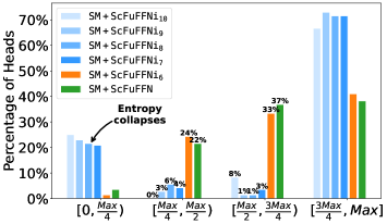
Figure 15: Head-wise entropy distribution in the Softmax-only GPT-2 model ($L$=12, $H$=12, $d$=768) with earlier FFNs intact and deeper FFNs pruned, trained from scratch on the CodeParrot dataset.

To further reduce the FLOPs in the ${\tt SM+ScFuFFN}$ model, where each FFN is simplified to a single fused linear layer, we experimented with gradually pruning the deeper FFNs by replacing them with identity connections and monitoring training stability. Figure 15 presents a comparison of headwise entropy distributions between the pruned and unpruned models, both trained from scratch. Instability emerged when more than 6 deeper FFNs were pruned, as indicated by a significant shift in the headwise entropy distribution. Specifically, we observed entropy collapse, where a disproportionate number of attention heads exhibited extremely low entropy values, ranging from 0 to $\frac{\tt Max}{4}$, with most values near zero. Less than 10% of the attention heads maintained entropy values in the balanced range of $\frac{\tt Max}{4}$ to $\frac{3\tt Max}{4}$. This highlights the critical role of earlier FFNs in stabilizing the training of the model, even when reduced to linear transformations.

To investigate this instability further, Figure 16 provides a detailed analysis. Training stability is maintained when up to 6 FFNs are pruned, as shown by the layer-wise entropy dynamics and heatmaps, which resembles the behavior of the unpruned ${\tt SM+ScFuFFN}$ model. In particular, both models have approximately 55% to 60% of attention heads exhibiting entropy values in the balanced range, with negligible attention heads falling within the 0 to $\frac{\tt Max}{4}$ range. However, pruning the 7th FFN (${\tt SM+ScFuFFNi_{7}}$) leads to a sudden shift, resulting in NaNs and entropy collapse, particularly in the deeper layers. The similarity in entropy dynamics and heatmaps between the stable configurations suggests that the model remains robust as long as no more than 6 FFNs are pruned.

Nonetheless, all the pruned and unpruned models exhibit entropic overload, where a significant fraction of attention heads possess high entropy values in the range $\frac{3\tt Max}{4}$ to ${\tt Max}$, stable models exhibiting this overload to a lesser extent.

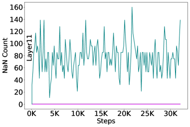
(a) Training instability (NaNs) in ${\tt SM+ScFuFFNi_{7}}$

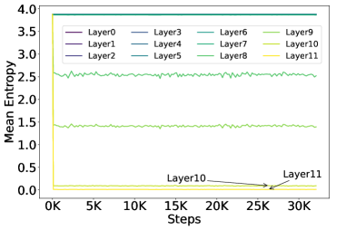
(b) Entropy collapses in ${\tt SM+ScFuFFNi_{7}}$

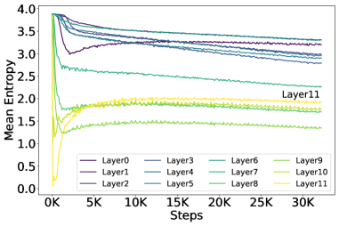
(c) Entropy dynamics in ${\tt SM+ScFuFFNi_{6}}$

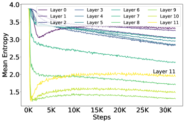
(d) Entropy dynamics in ${\tt SM+ScFuFFN}$

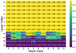
(e) ${\tt SM+ScFuFFNi_{7}}$

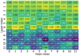
(f) ${\tt SM+ScFuFFNi_{6}}$

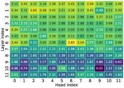
(g) ${\tt SM+ScFuFFN}$

Figure 16: Training instability is evident with NaNs in the final layers (a) and entropy collapse in the last two layers (b) of the ${\tt SM+ScFuFFNi_{7}}$ configuration, where 7 deeper FFNs are pruned in the Softmax-only GPT-2 model ($L$ = 12, $H$ = 12, $d$ = 768), trained from scratch on the CodeParrot dataset. In contrast, stable training is observed in (c) with no entropy collapse when only 6 deeper FFNs are pruned (${\tt SM+ScFuFFNi_{6}}$), and further validated against the unpruned configuration (${\tt SM+ScFuFFN}$) in (d). The last row (e, f, g) shows entropy heatmaps for each configuration.

D.8 Mitigating Over-Regularization with an Appropriate Threshold Margin

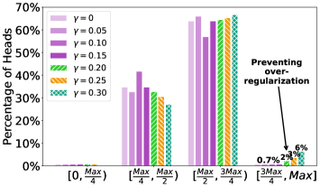
Figure 17: Headwise entropy distribution in the ${\tt SM(t)+ScFuFFN}$ GPT-2 model ($L$=12, $H$=12, $d$=768) when entropy regularization is applied with varying threshold margin, controlled by hyperparameter $\gamma$.

Figure 17 illustrates the effect of $\gamma$ on the headwise entropy distribution. The hyperparameter $\gamma$ employed to adjust the threshold margin in entropy regularization, defined as $\text{Tol}_{\text{margin}}=\gamma\text{E}_{\text{max}}$ (Algorithm1, line #3), effectively preventing over-regularization by ensuring that a sufficient fraction of heads maintains entropy values in the upper range $\frac{\tt 3Max}{4}$ to ${\tt Max}$. As $\gamma$ increases from 0 to 0.15, only a small proportion of attention heads (0.7%) are situated in the highest entropy range. However, as $\gamma$ is increased beyond 0.15, the fraction of heads in this upper range starts increasing, reaching 2.08%, 3.47%, and 6.25% at $\gamma$=0.20, 0.25, and 0.30, respectively. This fine-grained control on the population of attention heads in the higher entropy range highlights the ability of entropy regularization to prevent over-regularization and maintain the attention heads’ diversity. We find that $\gamma$=0.2 yields slightly better performance in terms of lower perplexity compared to higher $\gamma$ values, and thus, we adopt this value in the final entropy regularization scheme.

To better understand the increase in the fraction of attention heads with higher $\gamma$, Figure 18 illustrates the layerwise entropy dynamics during training. Notably, at higher $\gamma$, the fraction of attention heads with higher entropy values increases, as indicated by the increases in the mean entropy of the early layers, which helps to prevent over-regularization and maintain heads’ diversity.

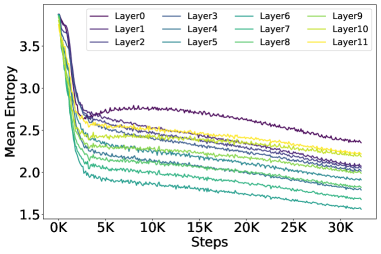
(a) $\text{Tol}_{\text{margin}}=0.15\text{E}_{\text{max}}$

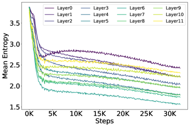
(b) $\text{Tol}_{\text{margin}}=0.20\text{E}_{\text{max}}$

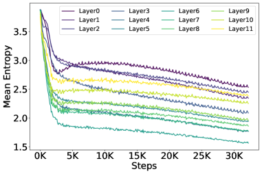
(c) $\text{Tol}_{\text{margin}}=0.25\text{E}_{\text{max}}$

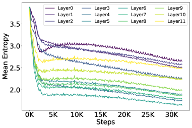
(d) $\text{Tol}_{\text{margin}}=0.30\text{E}_{\text{max}}$

Figure 18: Layerwise entropy dynamics when entropy regularization is employed with increasing threshold margin, defined as $\text{Tol}_{\text{margin}}=\gamma\text{E}_{\text{max}}$ (see Algorithm1, line #3). At higher $\gamma$, the mean entropy of the early layers increases.

Appendix E FLOPs Computation for Inference

To generate one output token during inference, the model performs a forward pass over a sequence of length $L$ (the context size). Below, we detail the FLOPs required for both the feed-forward (FFN) and self-attention sub-blocks. We compute the FLOPs per token per layer as follows:

• FFN FLOPs: The FFN sub-block consists of two linear transformations, parameterized by $\mathbf{W}^{\text{ffn}}_{\text{in}}\in\mathbb{R}^{d\times 4d}$ and $\mathbf{W}^{\text{ffn}}_{\text{out}}\in\mathbb{R}^{4d\times d}$. Each layer contributes equally to the FLOPs count. The total FLOPs for the FFN can be expressed as:

  $$\text{FFN FLOPs}=2\times 2\times(d\times 4d)=16d^{2}$$

  
  

  - The first factor of 2 accounts for the two linear layers, while the second factor of 2 arises because each dot product in a matrix-matrix multiplication involves two floating point operations—one multiplication and one addition (Performance, 2023).
  

• Self-Attention FLOPs: The breakdown for attention FLOPs is presented as follows:

  1. Linear projections (W^Q, W^K, W^V, and W^O) FLOPs: The input sequence of shape $\mathbb{R}^{T\times d}$ is linearly transformed using weights of shape $\mathbb{R}^{d\times d}$ across four linear layers (for queries, keys, values, and output projection). Thus, the total FLOPs for these operations are:

     $$4\times 2\times T\times(d\times d)=8Td^{2}$$

     Since we are interested in FLOPs per token, this simplifies to $8d^{2}$

  2. Attention Matrix (QK^T) Computation: The attention mechanism involves computing the dot product between the query matrix $\mathbf{Q}\in\mathbb{R}^{T\times d_{k}}$ and the transposed key matrix $\mathbf{K}^{T}\in\mathbb{R}^{d_{k}\times T}$. For each attention head, this operation results in:

     $$2\times T\times d_{k}\times T$$

     With $H$ heads, the total FLOPs for this step are:

     $$2\times H\times(T\times d_{k}\times T)=2dT^{2}$$

     Hence, FLOPs per token simplifies to $2dT$.

  3. Dot Product with V: After calculating the attention weights, the values matrix $\mathbf{V}\in\mathbb{R}^{T\times d_{k}}$ is multiplied by the attention scores. Due to the masking in the upper triangular attention matrix (to enforce causality), only the lower triangular part of the matrix is involved in the computation. The number of FLOPs per head is:

     $$2\times d_{k}\times\frac{T(T+1)}{2}$$

     For $H$ heads, this totals to:

     $$2\times d\times\frac{T(T+1)}{2}$$

     Thus, the FLOPs per token for this step are:

     $$d\times(T+1)$$

  Combining all components, the total FLOPs for self-attention per token is:

  $$\text{Self-attention FLOPs}=8d^{2}+2Td+d(T+1)$$

In summary, the FLOPs computation for one layer includes both the FFN and self-attention sub-blocks, yielding the following total per token:

$$\text{Total FLOPs per token per layer}=\underbrace{16d^{2}}_{\text{FFN}}+\underbrace{(8d^{2}+3Td+d)}_{\text{Self-attention}}$$

$$\text{Total FLOPs with $L$ layers and $T$ tokens (context length) }=L\times T\times(24d^{2}+3Td+d)$$

Note that the FFN FLOPs depend on the hidden dimension, a design hyperparameter typically set as a multiple of the model dimension $d$, which varies across LLM architectures, for example, $4d$ in GPT-2 (Radford et al., 2019; Brown et al., 2020) and Pythia(Biderman et al., 2023), $\frac{8d}{3}$ in LLaMA(Touvron et al., 2023), $3.5d$ in Mistral Jiang et al. (2023), and $8d$ in Gemma Team et al. (2024).

Now, we want to analyze which component, FFN or self-attention, dominates the total FLOPs count of a given architecture. For this, we solve the following inequality:

$$16d^{2} >8d^{2}+3dT+d\implies 8d^{2}>d(3T+1)\implies 8d-1>3T\implies T<\frac{8d-1}{3}$$

$$\implies T <\frac{8d}{3}\quad\quad\text{(To simplify, we approximate $8d-1\approx 8d$)}$$ (13)

It is evident that in the shorter context length regime, where $T<\frac{8d}{3}$, the FFN FLOPs dominate the total FLOPs. Thus, for tasks with smaller context lengths, optimizing the FFN sub-block can lead to efficiency gains, while for larger contexts, self-attention FLOPs become more significant. Therefore, understanding this FLOPs distribution can guide efficient architectural design for private inference, depending on the expected context size.

E.1 Distribution of FLOPs in GPT-2 Models

Figure 19 illustrates the distribution of FLOPs between the attention and FFN sub-blocks across different context sizes for GPT-2 models, ranging from 128 to 8K tokens.

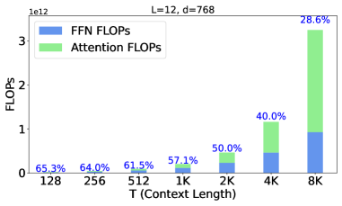
(a) GPT-2 small

(b) GPT-2 medium

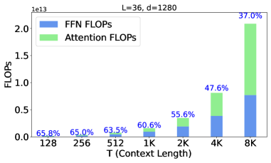
(c) GPT-2 large

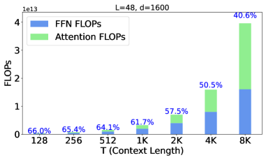
(d) GPT-2 XL

Figure 19: FLOPs breakdown in GPT-2 models for a single forward pass: Up to a context length of 2K, FFN operations are the primary contributors to FLOPs. Beyond 8K, attention operations start to dominate (Percentage on top of each bar represents the proportion of FFN FLOPs)

E.2 Distribution of FLOPs in Pythia Models

Figure 20 illustrates the distribution of FLOPs between the attention and FFN sub-blocks across different context sizes for Pythia models, ranging from 128 to 8K tokens.

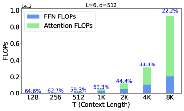
(a) Pythia-70M

(b) Pythia-160M

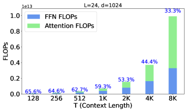
(c) Pythia-410M

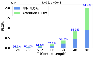
(d) Pythia-1B

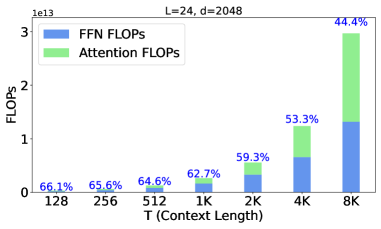
(e) Pythia-1.4B

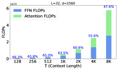
(f) Pythia-2.8B

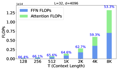
(g) Pythia-6.9B

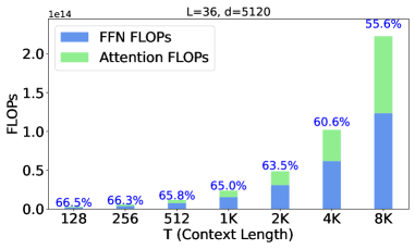
(h) Pythia-12B

Figure 20: FLOPs breakdown in Pythia models for a single forward pass: Similar to GPT-2 models (see Figure 19), FLOPs are dominated by FFN operations up to a context length of 4K, except for smaller models where FFN operations dominate up to 2K (Percentage on top of each bar represents the proportion of FFN FLOPs).

Appendix F Additional Related Work

The Pitfalls of LayerNorm in LLM While LayerNorm is a critical source of non-linearity in both CNNs (Ni et al., 2024) and transformer-based models (Wu et al., 2024; Zhao et al., 2024; Joudaki et al., 2023), it causes several challenges in the transformer-based LLMs that extend well-beyond PI.

First, in PI with hybrid protocols, the inverse-square root computation poses significant challenges for its precise computation. Also, in HE-only PI, the polynomial approximation of LayerNorm is quite challenging because of the unusually wide range of its variance values Zimerman et al. (2024).

Furthermore, the trainable parameters in LayerNorm are shown to be associated with the outlier features in LLMs He et al. (2024); Bondarenko et al. (2023); Wei et al. (2022); Kovaleva et al. (2021), posing significant issues in LLM quantization. Specifically, the scaling parameters in LayerNorm amplify outlier features, which in turn makes low-precision training challenging Wei et al. (2022).

Moreover, LayerNorm introduces difficulties in mechanistic interpretability, as it tends to make the residual stream more complex and harder to analyze Nanda (2023).

Also, from the perspective of signal propagation theories, LayerNorm negatively impacts the trainability of LLMs He & Hofmann (2024); He et al. (2023).

Entropy Regularization Entropy regularization has been widely applied in various areas of machine learning. It has been used to penalize low entropy predictions (Pereyra et al., 2017) and to maximize predictions’ entropy (Setlur et al., 2022). It has also been used to improve adversarial robustness (Jagatap et al., 2022), to avoid bad initializations and local minima (Miller et al., 1996), to optimize the layer-wise flow of information in deeper networks (Peer et al., 2022), to balance exploration-exploitation and promote action diversity in reinforcement learning (Wang et al., 2024; Ahmed et al., 2019; Lu & Van Roy, 2019; Neu et al., 2017; Mnih, 2016), and for domain generalization (Zhao et al., 2020).

The Role of Nonlinearity in LLM Understanding the role of nonlinearity in the transformer-based models is an emerging research area. Li et al. (2024) offer a theoretical analysis on the role of attention and FFN nonlinearity for in-context learning tasks. However, their work is limited to a simplified, one-layer model consisting of a single softmax-based self-attention head and a ReLU-based FFN. Nonetheless, Cheng et al. (2024) explore a broader range of nonlinear architectures and in-context learning tasks, demonstrating that the optimal activation function can vary depending on the specific function class the model is attempting to learn.

Appendix G Discussion

G.1 Linear vs. Non-linear FFNs: Privileged Basis and Rotational Invariance

In transformer-based architectures, there is a crucial distinction between linear and non-linear transformations, particularly when analyzing the privileged basis phenomenon (Elhage et al., 2023).

A privileged basis occurs when certain directions in the network’s activation space are favored due to the network’s architecture. Specifically, non-linear activations (e.g., ReLU, GELU) encourage features to align with specific directions in the hidden space, breaking the rotational invariance of the network. This alignment forces neurons to prioritize specific directions or features, leading to a basis that is more interpretable but inherently dependent on the chosen non-linear function.

Non-linear FFN In a conventional FFN, the architecture includes two linear transformations with a non-linear activation between them. This non-linearity breaks the rotational invariance of the hidden space, as the activation function behaves differently depending on the input direction. Mathematically, this can be described as:

$$\text{FFN}_{\text{non-linear}}(x)=\sigma(x\mathbf{W}_{\text{in}}^{\text{ffn}}+\mathbf{b}_{1})\mathbf{W}_{\text{out}}^{\text{ffn}}+\mathbf{b}_{2}$$

Where $\sigma(\cdot)$ represents the elementwise non-linearity, which restricts the model from treating all directions in the hidden space equally, thereby establishing a privileged basis.

Linear FFN Removing the non-linearity from the FFN results in a purely linear transformation, which preserves rotational invariance in the hidden space. The linear FFN operates as:

$$\text{FFN}_{\text{linear}}(x)=(x\mathbf{W}_{\text{in}}^{\text{ffn}})\mathbf{W}_{\text{out}}^{\text{ffn}}+\mathbf{b}$$

Without the activation function, the representations remain invariant under rotations, meaning that no specific direction is favored over others. In a linear FFN, the model retains its flexibility in how it represents features, without forcing any particular alignment of neurons. In effect, the model operates in a non-privileged basis, allowing the representation to rotate freely in the vector space.

G.2 Early vs. Deeper FFNs

Early FFNs in transformer models are particularly critical due to the presence of polysemantic neurons(Ferrando et al., 2024), which can respond to multiple, unrelated features simultaneously. These neurons enable early layers to detect broad and diverse patterns, such as linguistic structures, n-grams, and other foundational features of the input. This general-purpose functionality allows the early FFNs to play a vital role in the initial stages of context formation, capturing a wide range of information necessary for effective processing in later stages.

Additionally, research highlights that early layers play a pivotal role in the memorization and recall of factual information (Haviv et al., 2023; Meng et al., 2022). These layers not only capture general patterns but also store and retrieve memorized knowledge, promoting the predicted token to the top of the output distribution. This suggests that early FFNs are integral for accessing learned information, making them crucial for both context formation and recalling facts essential to the model’s predictions.

In contrast, deeper FFNs become more specialized, focusing on refining the information extracted by the earlier layers. They process the data with a narrower scope, tailoring it for task-specific outputs. While these deeper layers are essential for fine-tuning the model’s predictions, the early FFNs are key to generalizing over complex and varied input patterns, establishing the groundwork for the model’s overall performance.

Appendix H Future Work

To further reduce non-linear operations in our Softmax-only architecture, off-the-shelf head pruning techniques Voita et al. (2019); Michel et al. (2019); Jo & Myaeng (2020); Ma et al. (2021); Li et al. (2022) can be applied on top of AERO. Another approach is to explore linear softmax operations. However, these linear softmax operations sometimes introduce additional normalization layers or complex activation functions in the FFN Zhang et al. (2024), which could increase the PI overheads, counteracting the intended efficiency improvements.

Additionally, incorporating weight and activation quantization Wu et al. (2023); Xiao et al. (2023); Dettmers & Zettlemoyer (2023) could further enhance the efficiency of private inference in our architecture.

Orthogonally, performance improvement techniques such as knowledge distillation (KD) can be employed to complement these optimizations Ko et al. (2024); Liang et al. (2023); Gu et al. (2023); Hsieh et al. (2023); Li et al. (2023b).

Looking ahead, scaling AERO to more complex and deeper LLMs can be achieved by strategically combining techniques such as weight normalization, spectral normalization, and FFN output scaling. These methods can be applied selectively, with different layers using different techniques—for instance, employing spectral normalization in early layers and FFN output scaling in deeper layers. This tailored approach could lead to better stability and efficiency in larger models.

References

- Achiam et al. (2023) Josh Achiam, Steven Adler, Sandhini Agarwal, Lama Ahmad, Ilge Akkaya, Florencia Leoni Aleman, Diogo Almeida, Janko Altenschmidt, Sam Altman, Shyamal Anadkat, et al. Gpt-4 technical report. arXiv preprint arXiv:2303.08774, 2023.
- Ahmed et al. (2019) Zafarali Ahmed, Nicolas Le Roux, Mohammad Norouzi, and Dale Schuurmans. Understanding the impact of entropy on policy optimization. In International conference on machine learning (ICML), 2019.
- Alleman et al. (2024) Matteo Alleman, Jack Lindsey, and Stefano Fusi. Task structure and nonlinearity jointly determine learned representational geometry. In The Twelfth International Conference on Learning Representations (ICLR), 2024.
- Baez (2024) John C. Baez. What is entropy? arXiv preprint arXiv:2409.09232, 2024. https://arxiv.org/abs/2409.09232.
- Biderman et al. (2023) Stella Biderman, Hailey Schoelkopf, Quentin Gregory Anthony, Herbie Bradley, Kyle O’Brien, Eric Hallahan, Mohammad Aflah Khan, Shivanshu Purohit, USVSN Sai Prashanth, Edward Raff, et al. Pythia: A suite for analyzing large language models across training and scaling. In International Conference on Machine Learning (ICML), 2023.
- Bondarenko et al. (2023) Yelysei Bondarenko, Markus Nagel, and Tijmen Blankevoort. Quantizable transformers: Removing outliers by helping attention heads do nothing. In Advances in Neural Information Processing Systems, 2023.
- Brown et al. (2020) Tom Brown, Benjamin Mann, Nick Ryder, Melanie Subbiah, Jared D Kaplan, Prafulla Dhariwal, Arvind Neelakantan, Pranav Shyam, Girish Sastry, Amanda Askell, et al. Language models are few-shot learners. Advances in neural information processing systems, 2020.
- Carlini et al. (2024) Nicholas Carlini, Daniel Paleka, Krishnamurthy Dj Dvijotham, Thomas Steinke, Jonathan Hayase, A Feder Cooper, Katherine Lee, Matthew Jagielski, Milad Nasr, Arthur Conmy, et al. Stealing part of a production language model. In International Conference on Machine Learning (ICML), 2024.
- Chen et al. (2023) Dake Chen, Yuke Zhang, Souvik Kundu, Chenghao Li, and Peter A Beerel. Rna-vit: Reduced-dimension approximate normalized attention vision transformers for latency efficient private inference. In IEEE/ACM International Conference on Computer Aided Design (ICCAD), 2023.
- Cheng et al. (2024) Xiang Cheng, Yuxin Chen, and Suvrit Sra. Transformers implement functional gradient descent to learn non-linear functions in context. In Forty-first International Conference on Machine Learning (ICML), 2024.
- Dettmers & Zettlemoyer (2023) Tim Dettmers and Luke Zettlemoyer. The case for 4-bit precision: k-bit inference scaling laws. In International Conference on Machine Learning (ICML), 2023.
- Dhyani et al. (2024) Naren Dhyani, Jianqiao Mo, Patrick Yubeaton, Minsu Cho, Ameya Joshi, Siddharth Garg, Brandon Reagen, and Chinmay Hegde. Privit: Vision transformers for fast private inference. In Transactions on Machine Learning Research (TMLR), 2024.
- Elhage et al. (2023) Nelson Elhage, Robert Lasenby, and Christopher Olah. Privileged bases in the transformer residual stream. Transformer Circuits Thread, 2023.
- (14) Hugging Face. Codeparrot. https://huggingface.co/learn/nlp-course/chapter7/6.
- Ferrando et al. (2024) Javier Ferrando, Gabriele Sarti, Arianna Bisazza, and Marta R Costa-jussà. A primer on the inner workings of transformer-based language models. arXiv preprint arXiv:2405.00208, 2024.
- Geiping & Goldstein (2023) Jonas Geiping and Tom Goldstein. Cramming: Training a language model on a single gpu in one day. In International Conference on Machine Learning (ICML), 2023.
- Ghader & Monz (2017) Hamidreza Ghader and Christof Monz. What does attention in neural machine translation pay attention to? In Proceedings of the The 8th International Joint Conference on Natural Language Processing, 2017.
- Gu et al. (2023) Yuxian Gu, Li Dong, Furu Wei, and Minlie Huang. Minillm: Knowledge distillation of large language models. In The Twelfth International Conference on Learning Representations (ICLR), 2023.
- Gupta et al. (2024) Kanav Gupta, Neha Jawalkar, Ananta Mukherjee, Nishanth Chandran, Divya Gupta, Ashish Panwar, and Rahul Sharma. SIGMA: secure GPT inference with function secret sharing. In Proceedings on Privacy Enhancing Technologies (PETs), 2024.
- Haviv et al. (2023) Adi Haviv, Ido Cohen, Jacob Gidron, Roei Schuster, Yoav Goldberg, and Mor Geva. Understanding transformer memorization recall through idioms. In Proceedings of the 17th Conference of the European Chapter of the Association for Computational Linguistics (EACL), 2023.
- He & Hofmann (2024) Bobby He and Thomas Hofmann. Simplifying transformer blocks. In The Twelfth International Conference on Learning Representations (ICLR), 2024.
- He et al. (2023) Bobby He, James Martens, Guodong Zhang, Aleksandar Botev, Andrew Brock, Samuel L Smith, and Yee Whye Teh. Deep transformers without shortcuts: Modifying self-attention for faithful signal propagation. In The Eleventh International Conference on Learning Representations (ICLR), 2023.
- He et al. (2024) Bobby He, Lorenzo Noci, Daniele Paliotta, Imanol Schlag, and Thomas Hofmann. Understanding and minimising outlier features in neural network training. In Advances in Neural Information Processing Systems (NeurIPS), 2024.
- Hou et al. (2023) Xiaoyang Hou, Jian Liu, Jingyu Li, Yuhan Li, Wen-jie Lu, Cheng Hong, and Kui Ren. Ciphergpt: Secure two-party gpt inference. Cryptology ePrint Archive, 2023.
- Hsieh et al. (2023) Cheng-Yu Hsieh, Chun-Liang Li, Chih-Kuan Yeh, Hootan Nakhost, Yasuhisa Fujii, Alexander Ratner, Ranjay Krishna, Chen-Yu Lee, and Tomas Pfister. Distilling step-by-step! outperforming larger language models with less training data and smaller model sizes. In Annual Meeting of the Association for Computational Linguistics (ACL), 2023.
- Hu et al. (2024) Chenhui Hu, Pengfei Cao, Yubo Chen, Kang Liu, and Jun Zhao. Wilke: Wise-layer knowledge editor for lifelong knowledge editing. In Findings of the Association for Computational Linguistics (ACL), 2024.
- Hutchins et al. (2022) DeLesley Hutchins, Imanol Schlag, Yuhuai Wu, Ethan Dyer, and Behnam Neyshabur. Block-recurrent transformers. In Advances in neural information processing systems (NeurIPS), 2022.
- Jagatap et al. (2022) Gauri Jagatap, Ameya Joshi, Animesh Basak Chowdhury, Siddharth Garg, and Chinmay Hegde. Adversarially robust learning via entropic regularization. In Frontiers in artificial intelligence, 2022.
- Jaynes (1957) Edwin T Jaynes. Information theory and statistical mechanics. Physical review, 1957.
- Jaynes (1982) Edwin T Jaynes. On the rationale of maximum-entropy methods. In Proceedings of the IEEE, 1982.
- Jelinek et al. (1977) Fred Jelinek, Robert L Mercer, Lalit R Bahl, and James K Baker. Perplexity—a measure of the difficulty of speech recognition tasks. The Journal of the Acoustical Society of America, 1977.
- Jiang et al. (2023) Albert Q Jiang, Alexandre Sablayrolles, Arthur Mensch, Chris Bamford, Devendra Singh Chaplot, Diego de las Casas, Florian Bressand, Gianna Lengyel, Guillaume Lample, Lucile Saulnier, et al. Mistral 7b. arXiv preprint arXiv:2310.06825, 2023.
- Jin et al. (2024) Zhuoran Jin, Pengfei Cao, Hongbang Yuan, Yubo Chen, Jiexin Xu, Huaijun Li, Xiaojian Jiang, Kang Liu, and Jun Zhao. Cutting off the head ends the conflict: A mechanism for interpreting and mitigating knowledge conflicts in language models. In Findings of the Association for Computational Linguistics (ACL), 2024.
- Jo & Myaeng (2020) Jae-young Jo and Sung-Hyon Myaeng. Roles and utilization of attention heads in transformer-based neural language models. In Proceedings of the 58th Annual Meeting of the Association for Computational Linguistics, 2020.
- Joudaki et al. (2023) Amir Joudaki, Hadi Daneshmand, and Francis Bach. On the impact of activation and normalization in obtaining isometric embeddings at initialization. In Advances in Neural Information Processing Systems (NeurIPS), 2023.
- Jovanović et al. (2024) Nikola Jovanović, Robin Staab, and Martin Vechev. Watermark stealing in large language models. In International Conference on Machine Learning (ICML), 2024.
- Knott et al. (2021) Brian Knott, Shobha Venkataraman, Awni Hannun, Shubho Sengupta, Mark Ibrahim, and Laurens van der Maaten. Crypten: Secure multi-party computation meets machine learning. Advances in Neural Information Processing Systems, 2021.
- Ko et al. (2024) Jongwoo Ko, Sungnyun Kim, Tianyi Chen, and Se-Young Yun. Distillm: Towards streamlined distillation for large language models. In International Conference on Machine Learning (ICML), 2024.
- Kobayashi et al. (2024) Goro Kobayashi, Tatsuki Kuribayashi, Sho Yokoi, and Kentaro Inui. Analyzing feed-forward blocks in transformers through the lens of attention map. In The Twelfth International Conference on Learning Representations (ICLR), 2024.
- Kovaleva et al. (2021) Olga Kovaleva, Saurabh Kulshreshtha, Anna Rogers, and Anna Rumshisky. Bert busters: Outlier dimensions that disrupt transformers. In Findings of the Association for Computational Linguistics (ACL-IJCNLP), 2021.
- Lauren & Knight (2023) Goode Lauren and Will Knight. Chatgpt can now talk to you—and look into your life. https://www.wired.com/story/chatgpt-can-now-talk-to-you-and-look-into-your-life/, 2023.
- Li et al. (2023a) Dacheng Li, Hongyi Wang, Rulin Shao, Han Guo, Eric Xing, and Hao Zhang. MPCFORMER: FAST, PERFORMANT AND PRIVATE TRANSFORMER INFERENCE WITH MPC. In The Eleventh International Conference on Learning Representations (ICLR), 2023a.
- Li et al. (2024) Hongkang Li, Meng Wang, Songtao Lu, Xiaodong Cui, and Pin-Yu Chen. How do nonlinear transformers learn and generalize in in-context learning? In Forty-first International Conference on Machine Learning (ICML), 2024.
- Li et al. (2023b) Liunian Harold Li, Jack Hessel, Youngjae Yu, Xiang Ren, Kai-Wei Chang, and Yejin Choi. Symbolic chain-of-thought distillation: Small models can also" think" step-by-step. In Annual Meeting of the Association for Computational Linguistics (ACL), 2023b.
- Li et al. (2022) Zheng Li, Soroush Ghodrati, Amir Yazdanbakhsh, Hadi Esmaeilzadeh, and Mingu Kang. Accelerating attention through gradient-based learned runtime pruning. In Proceedings of the 49th Annual International Symposium on Computer Architecture (ISCA), 2022.
- Liang et al. (2023) Chen Liang, Simiao Zuo, Qingru Zhang, Pengcheng He, Weizhu Chen, and Tuo Zhao. Less is more: Task-aware layer-wise distillation for language model compression. In International Conference on Machine Learning (ICML), 2023.
- Lu et al. (2025) Wen-jie Lu, Zhicong Huang, Zhen Gu, Jingyu Li, Jian Liu, Kui Ren, Cheng Hong, Tao Wei, and WenGuang Chen. Bumblebee: Secure two-party inference framework for large transformers. In Annual Network and Distributed System Security Symposium (NDSS), 2025.
- Lu et al. (2024) Xin Lu, Yanyan Zhao, and Bing Qin. How does architecture influence the base capabilities of pre-trained language models? a case study based on ffn-wider transformer models. In Advances in Neural Information Processing Systems (NeurIPS), 2024.
- Lu & Van Roy (2019) Xiuyuan Lu and Benjamin Van Roy. Information-theoretic confidence bounds for reinforcement learning. In Advances in Neural Information Processing Systems, 2019.
- Ma et al. (2021) Weicheng Ma, Kai Zhang, Renze Lou, Lili Wang, and Soroush Vosoughi. Contributions of transformer attention heads in multi- and cross-lingual tasks. In Annual Meeting of the Association for Computational Linguistics (ACL), 2021.
- Maas et al. (2013) Andrew L Maas, Awni Y Hannun, Andrew Y Ng, et al. Rectifier nonlinearities improve neural network acoustic models. In International Conference on Machine Learning (ICML), 2013.
- Meng et al. (2022) Kevin Meng, David Bau, Alex Andonian, and Yonatan Belinkov. Locating and editing factual associations in gpt. In Advances in Neural Information Processing Systems (NeurIPS), 2022.
- Michel et al. (2019) Paul Michel, Omer Levy, and Graham Neubig. Are sixteen heads really better than one? In Advances in neural information processing systems, 2019.
- Miller et al. (1996) David Miller, Ajit V Rao, Kenneth Rose, and Allen Gersho. A global optimization technique for statistical classifier design. IEEE transactions on signal processing, 1996.
- Mireshghallah et al. (2024) Niloofar Mireshghallah, Hyunwoo Kim, Xuhui Zhou, Yulia Tsvetkov, Maarten Sap, Reza Shokri, and Yejin Choi. Can LLMs keep a secret? testing privacy implications of language models via contextual integrity theory. In The Twelfth International Conference on Learning Representations, 2024.
- Miyato et al. (2018) Takeru Miyato, Toshiki Kataoka, Masanori Koyama, and Yuichi Yoshida. Spectral normalization for generative adversarial networks. In International Conference on Learning Representations (ICLR), 2018.
- Mnih (2016) Volodymyr Mnih. Asynchronous methods for deep reinforcement learning. In Proceedings of The 33rd International Conference on Machine Learning (ICML), 2016.
- Nahshan et al. (2024) Yury Nahshan, Joseph Kampeas, and Emir Haleva. Linear log-normal attention with unbiased concentration. In The Twelfth International Conference on Learning Representations (ICLR), 2024.
- Nanda (2023) Neel Nanda. Attribution patching: Activation patching at industrial scale. URL: https://www. neelnanda. io/mechanistic-interpretability/attribution-patching, 2023.
- Nanda et al. (2023) Neel Nanda, Senthooran Rajamanoharan, Janos Kramar, and Rohin Shah. Fact finding: Trying to mechanistically understanding early MLPs. https://www.alignmentforum.org/s/hpWHhjvjn67LJ4xXX/p/CW5onXm6uZxpbpsRk, December 2023.
- Neu et al. (2017) Gergely Neu, Anders Jonsson, and Vicenç Gómez. A unified view of entropy-regularized markov decision processes. arXiv preprint arXiv:1705.07798, 2017.
- Ni et al. (2024) Yunhao Ni, Yuxin Guo, Junlong Jia, and Lei Huang. On the nonlinearity of layer normalization. In Forty-first International Conference on Machine Learning (ICML), 2024.
- Noci et al. (2023) Lorenzo Noci, Chuning Li, Mufan Li, Bobby He, Thomas Hofmann, Chris J Maddison, and Dan Roy. The shaped transformer: Attention models in the infinite depth-and-width limit. Advances in Neural Information Processing Systems (NeurIPS), 2023.
- Pang et al. (2024) Qi Pang, Jinhao Zhu, Helen Möllering, Wenting Zheng, and Thomas Schneider. Bolt: Privacy-preserving, accurate and efficient inference for transformers. In IEEE Symposium on Security and Privacy (SP), 2024.
- Peer et al. (2022) David Peer, Bart Keulen, Sebastian Stabinger, Justus Piater, and Antonio Rodriguez-sanchez. Improving the trainability of deep neural networks through layerwise batch-entropy regularization. In Transactions on Machine Learning Research (TMLR), 2022.
- Pereyra et al. (2017) Gabriel Pereyra, George Tucker, Jan Chorowski, Łukasz Kaiser, and Geoffrey Hinton. Regularizing neural networks by penalizing confident output distributions. arXiv preprint arXiv:1701.06548, 2017.
- Performance (2023) NVIDIA Deep Learning Performance. Matrix multiplication background user’s guide. https://docs.nvidia.com/deeplearning/performance/dl-performance-matrix-multiplication/index.html, 2023.
- Pires et al. (2023) Telmo Pessoa Pires, António V Lopes, Yannick Assogba, and Hendra Setiawan. One wide feedforward is all you need. In Proceedings of the Eighth Conference on Machine Translation, 2023.
- Priyanshu et al. (2023) Aman Priyanshu, Supriti Vijay, Ayush Kumar, Rakshit Naidu, and Fatemehsadat Mireshghallah. Are chatbots ready for privacy-sensitive applications? an investigation into input regurgitation and prompt-induced sanitization. arXiv preprint arXiv:2305.15008, 2023.
- Radford et al. (2019) Alec Radford, Jeffrey Wu, Rewon Child, David Luan, Dario Amodei, Ilya Sutskever, et al. Language models are unsupervised multitask learners. OpenAI blog, 2019.
- Salimans & Kingma (2016) Tim Salimans and Durk P Kingma. Weight normalization: A simple reparameterization to accelerate training of deep neural networks. In Advances in neural information processing systems, 2016.
- Setlur et al. (2022) Amrith Setlur, Benjamin Eysenbach, Virginia Smith, and Sergey Levine. Maximizing entropy on adversarial examples can improve generalization. In ICLR 2022 Workshop on PAIR^2Struct: Privacy, Accountability, Interpretability, Robustness, Reasoning on Structured Data, 2022.
- Shannon (1948) Claude Elwood Shannon. A mathematical theory of communication. The Bell system technical journal, 1948.
- Sharma et al. (2024) Pratyusha Sharma, Jordan T. Ash, and Dipendra Misra. The truth is in there: Improving reasoning with layer-selective rank reduction. In The Twelfth International Conference on Learning Representations (ICLR), 2024.
- Staab et al. (2024) Robin Staab, Mark Vero, Mislav Balunovic, and Martin Vechev. Beyond memorization: Violating privacy via inference with large language models. In The Twelfth International Conference on Learning Representations (ICLR), 2024.
- Stanić et al. (2023) Aleksandar Stanić, Dylan Ashley, Oleg Serikov, Louis Kirsch, Francesco Faccio, Jürgen Schmidhuber, Thomas Hofmann, and Imanol Schlag. The languini kitchen: Enabling language modelling research at different scales of compute. arXiv preprint arXiv:2309.11197, 2023.
- Stolfo et al. (2023) Alessandro Stolfo, Yonatan Belinkov, and Mrinmaya Sachan. A mechanistic interpretation of arithmetic reasoning in language models using causal mediation analysis. In Empirical Methods in Natural Language Processing (EMNLP), 2023.
- Team et al. (2024) Gemma Team, Thomas Mesnard, Cassidy Hardin, Robert Dadashi, Surya Bhupatiraju, Shreya Pathak, Laurent Sifre, Morgane Rivière, Mihir Sanjay Kale, Juliette Love, et al. Gemma: Open models based on gemini research and technology. arXiv preprint arXiv:2403.08295, 2024.
- Touvron et al. (2023) Hugo Touvron, Thibaut Lavril, Gautier Izacard, Xavier Martinet, Marie-Anne Lachaux, Timothée Lacroix, Baptiste Rozière, Naman Goyal, Eric Hambro, Faisal Azhar, et al. Llama: Open and efficient foundation language models. arXiv preprint arXiv:2302.13971, 2023.
- Vig & Belinkov (2019) Jesse Vig and Yonatan Belinkov. Analyzing the structure of attention in a transformer language model. In Proceedings of the 2019 ACL Workshop BlackboxNLP: Analyzing and Interpreting Neural Networks for NLP, 2019.
- Voita et al. (2019) Elena Voita, David Talbot, Fedor Moiseev, Rico Sennrich, and Ivan Titov. Analyzing multi-head self-attention: Specialized heads do the heavy lifting, the rest can be pruned. In Proceedings of the 57th Annual Meeting of the Association for Computational Linguistics (ACL), 2019.
- Wang et al. (2023) Kevin Ro Wang, Alexandre Variengien, Arthur Conmy, Buck Shlegeris, and Jacob Steinhardt. Interpretability in the wild: a circuit for indirect object identification in GPT-2 small. In The Eleventh International Conference on Learning Representations (ICLR), 2023.
- Wang et al. (2024) Yinuo Wang, Likun Wang, Yuxuan Jiang, Wenjun Zou, Tong Liu, Xujie Song, Wenxuan Wang, Liming Xiao, Jiang Wu, Jingliang Duan, et al. Diffusion actor-critic with entropy regulator. In Advances in Neural Information Processing Systems (NeurIPS), 2024.
- Wei et al. (2022) Xiuying Wei, Yunchen Zhang, Xiangguo Zhang, Ruihao Gong, Shanghang Zhang, Qi Zhang, Fengwei Yu, and Xianglong Liu. Outlier suppression: Pushing the limit of low-bit transformer language models. In Advances in Neural Information Processing Systems, 2022.
- Wu et al. (2023) Xiaoxia Wu, Cheng Li, Reza Yazdani Aminabadi, Zhewei Yao, and Yuxiong He. Understanding int4 quantization for language models: latency speedup, composability, and failure cases. In International Conference on Machine Learning (ICML), 2023.
- Wu et al. (2024) Xinyi Wu, Amir Ajorlou, Yifei Wang, Stefanie Jegelka, and Ali Jadbabaie. On the role of attention masks and layernorm in transformers. In Advances in Neural Information Processing Systems (NeurIPS), 2024.
- Xiao et al. (2023) Guangxuan Xiao, Ji Lin, Mickael Seznec, Hao Wu, Julien Demouth, and Song Han. Smoothquant: Accurate and efficient post-training quantization for large language models. In International Conference on Machine Learning (ICML), 2023.
- Xiong et al. (2020) Ruibin Xiong, Yunchang Yang, Di He, Kai Zheng, Shuxin Zheng, Chen Xing, Huishuai Zhang, Yanyan Lan, Liwei Wang, and Tieyan Liu. On layer normalization in the transformer architecture. In International Conference on Machine Learning (ICML), 2020.
- Zeng et al. (2023) Wenxuan Zeng, Meng Li, Wenjie Xiong, Wenjie Lu, Jin Tan, Runsheng Wang, and Ru Huang. Mpcvit: Searching for mpc-friendly vision transformer with heterogeneous attention. In Proceedings of the IEEE/CVF International Conference on Computer Vision (ICCV), 2023.
- Zhai et al. (2023) Shuangfei Zhai, Tatiana Likhomanenko, Etai Littwin, Dan Busbridge, Jason Ramapuram, Yizhe Zhang, Jiatao Gu, and Joshua M Susskind. Stabilizing transformer training by preventing attention entropy collapse. In International Conference on Machine Learning (ICML), 2023.
- Zhang et al. (2025) Jiawen Zhang, Jian Liu, Xinpeng Yang, Yinghao Wang, Kejia Chen, Xiaoyang Hou, Kui Ren, and Xiaohu Yang. Secure transformer inference made non-interactive. In Annual Network and Distributed System Security Symposium (NDSS), 2025.
- Zhang et al. (2024) Michael Zhang, Kush Bhatia, Hermann Kumbong, and Christopher Re. The hedgehog & the porcupine: Expressive linear attentions with softmax mimicry. In The Twelfth International Conference on Learning Representations (ICLR), 2024.
- Zhang et al. (2023) Yuke Zhang, Dake Chen, Souvik Kundu, Chenghao Li, and Peter A. Beerel. Sal-vit: Towards latency efficient private inference on vit using selective attention search with a learnable softmax approximation. In Proceedings of the IEEE/CVF International Conference on Computer Vision (ICCV), 2023.
- Zhao et al. (2024) Bingchen Zhao, Haoqin Tu, Chen Wei, Jieru Mei, and Cihang Xie. Tuning LayerNorm in attention: Towards efficient multi-modal llm finetuning. In International Conference on Learning Representations (ICLR), 2024.
- Zhao et al. (2020) Shanshan Zhao, Mingming Gong, Tongliang Liu, Huan Fu, and Dacheng Tao. Domain generalization via entropy regularization. In Advances in neural information processing systems (NeurIPS), 2020.
- Zimerman et al. (2024) Itamar Zimerman, Moran Baruch, Nir Drucker, Gilad Ezov, Omri Soceanu, and Lior Wolf. Converting transformers to polynomial form for secure inference over homomorphic encryption. In International Conference on Machine Learning (ICML), 2024.