Explainable Binary Classification of Separable Shape Ensembles

Abstract

Materials scientists utilize image segmentation of micrographs to create large curve ensembles representing grain boundaries of material microstructures. Observations of these collections of shapes can facilitate inferences about material properties and manufacturing processes. We seek to bolster this application, and related engineering/scientific tasks, using novel pattern recognition formalisms and inference over large ensembles of segmented curves—i.e., facilitate principled assessments for quantifying differences in distributions of shapes. To this end, we apply a composite integral operator to motivate accurate and efficient numerical representations of discrete planar curves over matrix manifolds. The main result is a rigid-invariant orthonormal decomposition of curve component functions into separable forms of scale variations and complementary features of undulation. We demonstrate how these separable shape tensors—given thousands of curves in an ensemble—can inform explainable binary classification of segmented images by utilizing a product maximum mean discrepancy to distinguish the shape distributions; absent labelled data, building interpretable feature spaces in seconds without high performance computation, and detecting discrepancies below cursory visual inspections.

1 Problem Statement & Introduction

A variety of applications require the precise measurement and quantification of shape. Often these applications involve engineering design [29, 13], materials science [3, 4, 17, 18], medical imaging [43, 15], sensing and functional analysis [60, 59], biology [32, 53, 31], and ecology [42, 26], for example. Many of these applications benefit from separate parametrizations of shape planar translations (where is it?), scale variations (how big is it?), rotations/reflections (how is it oriented?), and everything else that remains (how nonlinear is it?). In several applications, a choice of invariance against one or multiple of the former similarity transforms [40]—among other transformations [7]—is beneficial for defining shape. And in a variety of applications, scientists and engineers simply want to ask a binary question: is this the same as that? But often necessitate some explanation: if they’re different, why? We refer to solutions of this general class of problems as explainable binary classifications.

In our materials application, electron backscatter diffraction (EBSD) [52] of material samples can offer high resolution image segmentation of the material’s microstructure [50, 54]. In particular, denoised images [3] and subsequent segmentation [5, 18] lead to a large ensemble of planar curves as data. An example of a segmented EBSD scan with deformed ice, utilizing an open-source software called MTEX [33, 17, 18], is shown in Figure 1. The segmented image in Figure 1 is juxtaposed to an example ‘grain boundary’ or, simply, ‘grain’ representing a single extracted planar curve from the tiled ensemble. An important question posed by materials scientists:

Are the grains in one EBSD scan, up to rigid transformations, the same or different from that of another and, if they are different, are differences due to scales (linear deformations) or undulations (nonlinear deformations)?

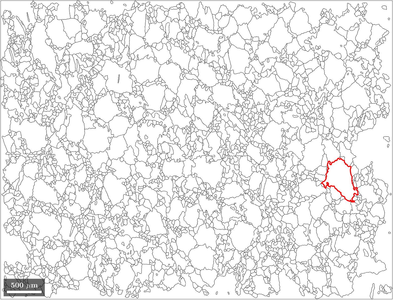
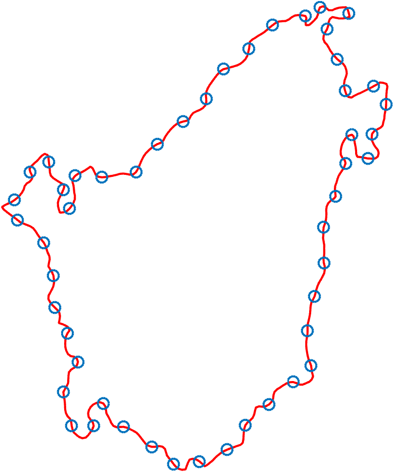
Figure 1: An ensemble of thousands of grain boundaries from an EBSD scan [18, 17] (left) and an example segmented grain boundary (right) with arc-length reparametrization landmarks (blue circles) generated by an interpolating curve (red). Data is available online [17].

Measuring these rigid-invariant differences is anticipated to have dramatic implications on the resulting macroscopic properties of the manufactured material—e.g., strength, ductility, and/or fracture behavior. We present a first attempt to guide binary classification of EBSD measurements with explainable methods and formal interpretations. This is in contrast to a more general class of artificial intelligence models that may accomplish a similar task if provided with labeled data but often lack quantifiable explanations due to the opaque nature of the ‘learned features’ defined over some ‘latent space.’

The notion of ‘difference’ in this context is statistical given the stochastic nature by which material grains form and evolve, as depicted in Figure 1. In other words, a naïve deterministic perspective that assesses if ensembles of shapes in different micrographs are identical with respect to some metric/distance is uninformative since no two sampled micrographs are ever the same—leading to limited conclusions in this presumed stochastic materials application.

Moreover, materials scientists often utilize expertise and visual inspection to suggest simple characteristics, e.g., principal lengths, area, perimeter, size, curvature, sphericity, and other shape factors, vary from one micrograph to the next [54, 36, 35, 37]. While such quantities can provide a cursory description of the ensemble characteristics, these handpicked features of shape do not constitute full representations of shape. Despite this, certain standards [39, 36, 35, 37] have been authored to detect hand-picked features. We expect our shape representations will offer dramatic improvements and insights for future standards in conjunction with existing hand-picked features.

The stochastic notion of difference in this application is based on (maximum mean) discrepancy: are the approximated distributions of representative shape features over the ensemble in one image statistically significant from the ensemble in another? To answer this question, we first i) represent shapes augmented by separating important distinguishing features, ii) discretize to approximate feature distributions of the shapes from both images, and finally iii) test for statistically significant discrepancies in distributions between two EBSD ensembles. This final step is referred to as a two-sample test [27]. For the application under consideration, this corresponds to statistically comparing thousands of shapes in two ensembles given two EBSD images.

It is important to note that shape is only one significant piece of the quite literal puzzle in Figure 1. However, for this work, we ignore the role of textures intrinsic to the tiling—i.e., the spatial arrangement of the shapes—and instead treat the ensemble of shapes as independent realizations from some generating distribution.

1.1 Technical Outline

Broadly, in Section 2, we formalize a continuous treatment of shapes as boundary curves to separately encode principled features of ‘generalized scale’ and ‘undulation.’ Then, in Section 3, we utilize accurate approximations of the formally developed shape features to test four logical combinations of statistical hypotheses with data. We supplement these tests with a novel analysis of maximum mean discrepancy (MMD) [27] offering interpretations for an explainable binary classification between two ensembles of separable shape features.

Specifically, we first motivate the concept of ‘preshape’ as the image of a curve in Subsection 1.3 and review a discrete treatment of shapes over matrix manifolds in Subsection 1.4—motivating that discretizations are simple quadratures given measurable curves. In Section 2, we offer a novel interpretation that discrete objects are approximations of dual representations over a vector-valued reproducing kernel Hilbert space (RKHS). Numerically, the discretizations are re-weighted to offer higher-order quadratures and discretizations become approximations of curve (dual) representations. Subsection 2.3 offers geometric interpretations of these infinite dimensional dual objects with simple examples.

With these formal interpretations, in Section 3 we explore numerical implications including: i) data alignment against an application-motivated archetypal shape, ii) numerical approximation of the eigen-problem as a square root quadrature decomposition, iii) an empirical regularizing effect via shape dimension reduction, and iv) logical implications of the two-sample statistical hypothesis test over separable parameters. Notably, in Subsection 3.4 we utilize discrete approximations of curve dual representations to learn parameter distributions (features) and discuss the implications of an explainable binary classification informed by MMD with separable, independent parameters. Finally, in Section 5, we conclude with a summary of results depicted in Figures 4-7 using measured materials and allude to future work.

1.2 Contributions

We emphasize the following contributions of this work: our explainable classification method i) does not require labeled data, ii) offers theoretical interpretations of learned features using dual representations of curves, and iii) results in a logical statistical classification over separable, independent parameters of shape. In contrast with AI methods, i) we don’t require challenging minimization over vast amounts of labeled training data (i.e., efficient implementation), ii) our feature/latent space is provably an approximation of dual representations of shape (i.e., mathematically interpretable), and iii) our classification is provably logical (i.e., some notion of trustworthy).

Our numerical experiments emphasize four scenarios where these tools deliver benefits: i) Figure 4 demonstrates that the method is not suspected to be overly sensitive to statistical rejection, ii) Figure 5 demonstrates that the method emulates conclusions consistent with human observations, iii) Figure 6 demonstrates that the method detects differences below human-scale visual observations and, iv) Figure 7 demonstrates that the method detects a presumed faulty measurement.

1.3 Preshapes as Boundary Curves

Preshapes are defined as open or closed curves $\bm{c}:\mathcal{I}\rightarrow\mathbb{R}^{d}$ assumed to be immersions and/or embeddings [44, 7, 53, 46, 63, 32]—e.g., for $d=2$, $\bm{c}$ in our application is a planar embedding with $\mathcal{I}$ as the unit circle or equivalent compact $(d-1)$-manifold. Applications are benefited by representations of curves over regularized Hilbert spaces which control noisy measurement oscillations, e.g., those with increasing Lipschitz constant of curves $\mathcal{C}(\lambda_{r})\subseteq\mathcal{C}(\lambda_{r+1})$ such that $\lambda_{r}\leq\lambda_{r+1}$ and

$$\mathcal{C}(\lambda_{r})\coloneqq\{\bm{c}\,:\,\|\bm{c}(u)-\bm{c}(s)\|\leq\lambda_{r}|u-s|\},$$ (1)

for all $u,s\in\mathcal{I}$, to explicitly control nonlinear undulations. Notice, it is sufficient to simply assume the individual components of curve $\bm{c}=(c_{1},c_{2},\dots,c_{d})$ are Lipschitz, such that $|c_{i}(u)-c_{i}(s)|\leq\lambda_{i,r}|u-s|$ with $\lambda_{r}=\|(\lambda_{1,r},\lambda_{2,r},\dots,\lambda_{d,r})^{\top}\|$. By the triangle inequality, this becomes a sufficient condition for bounding curves over a native Hilbert space with arbitrary choice of norm. We will generally refer to these curves as measurable curves for some $d\mu$, such that $\int_{\mathcal{I}}\|\bm{c}\|d\mu<\infty$, $\int_{\mathcal{I}}\|\dot{\bm{c}}\|d\mu<\infty$, and/or $\dot{\bm{c}}\neq 0$ as necessary, where $\dot{\bm{c}}$ represents the $d$ component-wise derivatives with respect to the curve parameter.

Note the assumption of differentiable curves in literature is a convenience for talking broadly about simple arc-length measures and arc-length reparametrizations. The core developments in this work only require measurable curves over a compact domain, which is sufficient to assume they are at least Lipschitz continuous per (1) but does not necessitate that curves be regular—similar to arguments in [53, 9].

We also remark that (1) is more restrictive than alternative assumptions on a space of grains which may be weakened to be at most continuous, of bounded variation, differentiable almost everywhere, or, quite possibly, fractal. However, the fundamental nature of grains is presently ambiguous as they are formed by complicated sub-atomic interactions driving rapid changes in phase [64]. Assumptions alluding to an appropriate space of curves are not clear from first principles. Consequently, any weakened treatment of assumptions on the space of curves, beyond (1), is desirable albeit difficult to assert from first principles.

Additionally, pre-processing in MTEX to extract curves from imaging implies a smoothing of grain boundaries with a suite of methods [34, 3] but inevitably results in a partition of the rectangular material area [6]. It is conceivable that segmented grains may admit a finite set of singularities as ‘corners’ or ‘junctions’—i.e., sets of measure zero where three boundaries meet or two boundaries depart, respectively, in the partition of the plane. However, if segmented grains are strictly piecewise smooth or polygonal due to a finite number of singularities on sets of measure zero, they are still appropriately measurable and applicable to our analysis [9]. In this case, convergence rates of subsequent approximations may be limited but this expense is minimal in comparison to the image processing.

Conversely, although singularities may be present in segmented grains by virtue of an algorithm which partitions the plane, physical grains may still be smooth to some extent—i.e., the singularities may be artificial and thus smoothing may constitute a correction. In this context, the physical nature of the problem may be one of packing smooth grain structures, not partitioning material areas. Regardless of the assumed regularity of curves, either perspective is flexibly managed in this presentation and we do not assert one perspective is more or less correct.

Our motivation is to relate novel interpretations of data objects over finite dimensional matrix manifolds to a functional analysis over an infinite dimensional RKHS. This interpretation facilitates a flexible choice of kernel which can be used to control the regularity of a Hilbert space of curves [44] hypothesized in any application.

When smooth representations are hypothesized, convenient, and beneficial—e.g., the reconstruction of reduced dimensional shapes depicted in Figure 3—we lean on Weierstrass approximation theorem to argue that the polynomial representations are still dense in the set of strictly continuous segmented grains over compact domains [58]. And given finite measurement precision in the imaging, we can get arbitrarily close (under measurement precision) with quasi-matrices [57, 55]. We also contend that strengthened regularity of curve interpolations can benefit the analysis by restricting numerics from walking into odd pathological issues, like curves with Cantor components [9] which are presumably not found in physical grains.

We can be flexible in the construction of a native/ambient space of curves utilizing any choice of norm or Sobolev-type metrics, which are crucial for controlling other pathological issues such as vanishing distances, over the (manifold) topologies of preshapes and shapes [45, 7, 44]. However, for now, $\mathcal{C}(\lambda_{r})$ defined with Euclidean $2$-norm is a simple choice that is consistent with the subsequent finite matrix manifolds of interest in related work involving Separable Shape Tensors (SST) [30], which we adopt for shape analysis in this paper.

Note, we are not attempting to build up a topology as a Riemannian manifold with $L^{2}(\mathcal{I})$ as a choice of metric. Instead, we expound on a class of integral operators defined by preshapes so that we may test statistical hypotheses, informed by an ensembles with thousands of curves, using discrete transformations of landmarks as data—and distances do not vanish over these finite dimensional manifolds [7]. One of our primary contributions is a formal interpretation of discrete transformations as dual representations of shape in M. Micheli and J. Glaunès [44]. We motivate novel explanations and extensions between our landmark configuration spaces defined as finite dimensional matrix product submanifolds of SST and the $\mathbb{R}^{d}$-valued RKHSs in [44] representing infinite dimensional features of curves.

1.4 Separable Shape Tensors

Next, we detail an approach for handling finite representations of curve data. Following the development of SST [30], first explored in an aerodynamic sensitivity analysis [28], we let $X=(\bm{x}_{1},\dots,\bm{x}_{n})^{\top}$ be the collection of $n$ unique landmarks informed by some $\bm{c}\in\mathcal{C}$ such that

$$\bm{x}_{i}=\bm{c}(s_{i}),\quad i=1,\dots,n.$$ (2)

Note that $X$ is assumed to be an element of the non-compact Stiefel manifold $\mathbb{R}^{n\times d}_{*}$ [1]. That is, in addition to assuming measurable (rectifiable) curves, we also assume $X\in\mathbb{R}^{n\times d}_{*}$ to exclude the degenerate cases of points or lines in $\mathbb{R}^{d}$ as objects representing curves [30]—necessitating that $X$ is full-rank. In other words, we assume the component functions $(c_{1},\dots,c_{d})$ of the curve are linearly independent.

In practice, we are often only given sequences of $n$ landmarks $(\bm{x}_{i})$ and have no knowledge of the ‘true’ (or universal) underlying $\bm{c}$ nor $s\in\mathcal{I}$ beyond the identification above. However, this characterization of the data implies landmarks are ordered according to some orientation of the unknown curve thus constituting a sequence, $(\bm{x}_{i})$, encoded over the row index of $X$. Thus, it is reasonable to build a variety of interpolations and approximations which can be shown to converge to the unknown $\bm{c}$ with an increasing number of given landmarks [30].

The method of SST proceeds by introducing a separable form of the curve into features of undulation and scale/rotation/shear/reflection as linear deformations for an aerodynamic design. Theoretical treatments of ‘discrete shapes’ as full-rank matrices [10] or complex vectors [40] offer geometric interpretations of the thin singular value decomposition (SVD),

$$(X-B(X))^{\top}\,\overset{SVD}{=}\,U\Sigma V^{\top},$$ (3)

with $B(X)=(1/n)\bm{1}_{n,n}X$, an unbiased centering operation, such that $\bm{1}_{n,n}\in\mathbb{R}^{n\times n}$ is a matrix of ones.

Given the SVD of $X$ representing a discrete shape, we can elaborate on related decompositions into complementary factors of (discrete) undulation and invertible $d$-by-$d$ linear deformations—i.e., in a complementary sense, an ‘undulation’ is the set of all shape representations which cannot be achieved by linear transforms as right group actions on $X-B(X)$. That is, ignoring non-deforming translations without loss of generality, for $\bm{c}(s)=M^{\top}\widetilde{\bm{c}}(s)$,

$$X^{\top} =(\bm{c}(s_{1}),\dots,\bm{c}(s_{n}))$$ (4)

$$=M^{\top}(\widetilde{\bm{c}}(s_{1}),\dots,\widetilde{\bm{c}}(s_{n}))$$

$$=(\widetilde{X}M)^{\top}$$

where the right action of $M\in\mathbb{GL}(d,\mathbb{R})$ on $\widetilde{X}=(\widetilde{\bm{c}}(s_{1}),\dots,\widetilde{\bm{c}}(s_{n}))^{\top}\in\mathbb{R}^{n\times d}_{*}$ is akin to linear deformations of the preshape. Given (centered) $X$, we seek a decomposition $X=\widetilde{X}M$ to describe how $X$ undulates as $[\widetilde{X}]$, an equivalence class modulo right group action over $\mathbb{GL}(d,\mathbb{R})$, versus how it linearly deforms over subsets of $M\in\mathbb{GL}(d,\mathbb{R})$. Therefore, we consider $[\widetilde{X}]\in Gr(d,n)$ such that $Gr(d,n)\cong\mathbb{R}^{n\times d}_{*}/\mathbb{GL}(d,\mathbb{R})$ as presented in [1].

We review two geometric interpretations of the SVD (3) called landmark standardizations [10, 30] to compute representative undulations $\widetilde{X}$ (up to rotations and reflections):

• The affine standardization [10] $X=\widetilde{X}M$ such that $\widetilde{X}\coloneqq V$ and $M\coloneqq\Sigma U^{\top}\in\mathbb{GL}^{+}(d,\mathbb{R})$.

• The polar standardization [30] $X=\widetilde{X}P$ such that $\widetilde{X}\coloneqq VU^{\top}$ and $P\coloneqq U\Sigma U^{\top}\in S^{d}_{++}$.

The latter polar standardization offers an interesting rigid-invariant decomposition for a variety of problems—specifically our materials application—which benefit from describing undulation and scale variations independent of rotations and reflections. In other words, following the development of [21], $S^{d}_{++}$ is identified with the set of equivalence classes given by the coset space $\mathbb{GL}^{+}(d,\mathbb{R})/\mathbb{SO}(d)$. Thus $[\widetilde{X}]$ encodes nonlinear features of shape over the quotient topology $\mathbb{R}^{n\times d}_{*}/\mathbb{GL}(d,\mathbb{R})$ as undulations while $P$ encodes generalized (unequal) scales independent of rotations and reflections over the quotient topology $\mathbb{GL}^{+}(d,\mathbb{R})/\mathbb{SO}(d)$.

Landmark standardization is thought to have a strong connection to the work of David G. Kendall et al. [40] albeit with distinct notions of scale. In our case, the definition of scale is generalized to all of $S^{d}_{++}$ as opposed to simple dilation of curves as a scalar multiplication to modulate overall size.

Given the SVD (3) and sought equivalence classes, the pairs $\{([\widetilde{X}],P)\}\in Gr(d,n)\times S^{d}_{++}$ inform a data-driven submanifold of the proposed product matrix-manifold to parametrize separable representations of shape tensors,

$$X(\bm{t},\bm{\ell})=\widetilde{X}(\bm{t})P(\bm{\ell}).$$ (5)

The parameters $\bm{t}\in\mathbb{R}^{r}$ are learned from the full ensemble of thousands of curves, from both images, and chosen with reduced dimension $r\leq d(n-d)$ according to a tangent space principal components analysis (tangent PCA) [20]. Additionally, full dimensional representation $\bm{\ell}\in\mathbb{R}^{3}$, learned with tangent PCA, govern generalized scale variations independent of rotations and reflections. The resulting representation (5) separates differences is scale variations, $P(\bm{\ell})$, from those of undulations, $[\widetilde{X}](\bm{t})$, utilizing a corresponding representative matrix, $\widetilde{X}(\bm{t})$, for computations [16, 30].

An important caveat of this finite representation is that shapes are not precluded from generating self-intersections—i.e., discrete shapes are generally identified with immersions. Moreover, the existing analysis is predicated on hand-picked discretizations of interpolating curves, called fixed reparametrizations [30], and lacks a formal interpretation of the entries of $\widetilde{X}$—other than achieving desirable aerodynamic parametrizations and subsequent meshing. This begs the question of how to relate the finite representation of (5) to an (infinite dimensional) analysis of continuous curves to offer improved discretizations and continuous extensions as embeddings.

2 Fredholm Integral Equation (FIE) of Curve

To formalize landmark standardization, we rearrange the SVD (3) into the symmetric counterpart as the (thin) scaled eigendecomposition, $(1/n)(X-B(X))(X-B(X))^{\top}\overset{s.v.d.}{=}(1/n)V\Sigma^{2}_{d}V^{\top}$—i.e., note the thin SVD implies $\Sigma_{d}$ is $d$-by-$d$, $\Sigma^{2}_{d}=\text{diag}(\sigma^{2}_{1},\dots,\sigma^{2}_{d})$ with $\sigma_{1}^{2}\geq\sigma_{2}^{2}\geq\dots\geq\sigma_{d}^{2}>0$. Next, we take a column partition $V=(\mathbb{v}_{1},\mathbb{v}_{2},\dots,\mathbb{v}_{d})$ where $V$ is an element of the Stiefel manifold and $V_{ij}=(v_{i})_{j}$ is the $i$-th (row), $i=1,\dots,n$, entry of the $j$-th (column) sequence, $j=1,\dots,d$. Equivalently, recalling in (2) that rows of the matrix are curve evaluations, the weighted eigendecomposition is expressed

$$\sum_{i=1}^{n}w_{i}(\bm{o}(s_{p})\cdot\bm{o}(s_{i}))(v_{i})_{j}\propto\sigma^{2}_{j}(v_{p})_{j},$$ (6)

where $w_{i}=1/n$ are constant (over $i$) weights in the sum, and $\bm{o}$ represents a fixed reparametrization of a ‘centered’ parametric curve generating data in the rows of $X-B(X)$, i.e., $X-B(X)=(\bm{o}(s_{1}),\dots,\bm{o}(s_{n}))^{\top}$.

Lemma 1.

Given a (centered) open or closed regular curve $\bm{o}:\mathcal{I}\rightarrow\mathbb{R}^{d}$ with unit-speed reparametrization, the symmetric counterpart of SVD (3) is proportional to an $O(n^{-1})$ quadrature such that $s_{i}\propto(i-1)/n$ or $O(n^{-2})$ quadrature such that $s_{i}\propto(2i-1)/2n$.

Proof.

A uniform sequence of quadrature nodes with weights $1/n$ over length-normalized unit-speed reparametrization, $s\in[0,1]$, admits a (left) Riemann sum with nodes $s_{i}=(i-1)/n$ converging generally at $O(n^{-1})$ or mid-point Riemann sum with nodes $s_{i}=(2i-1)/2n$ converging generally at $O(n^{-2})$. Note our convention for closed curves assumes $\bm{x}_{1}=\bm{x}_{n+1}$ is the duplicate point for the closure of the discrete polygonal form and is omitted from the sum over $n$ sub-intervals. And, for closed curves, both methods admit improved convergence reconciled by the periodicity of component functions [62]. More generally, convergence rates are limited to the case of open curves and the last (first) landmark is omitted from the left (right) Riemann sum. ∎

Lemma 1 offers a seemingly novel interpretation that specific landmark standardizations [10, 30] act as simple quadratures—albeit restricted to regular curves which our segmented grains may not satisfy prior to smoothing. However, generally any constant-weight quadrature rule over a fixed reparametrization according to arbitrary integral measure $d\mu(s)$ can be described as a scaling of (3) with an appropriate selection nodes $(s_{i})$ mapping to $(\bm{x}_{i})$—i.e., for strictly piecewise smooth curves consider a composite integral rule over knots of a spline coincident with the singularities. The motivation is not restricted by an assumption that curves must be regular but, instead, that (6) can be interpreted as a constant-weight quadrature for any measurable curve. However, with regular curve interpolations of data, we revisit this interpretation and generalize Lemma 1 by a spectral method for alternative approximations of closed, periodic curve representations in Section 2.1 offering a weighted landmark standardization. Otherwise, alternative quadratures can be sought.

Generalizing, for any measurable curve utilizing arbitrary integral measure $d\mu$, the interpretation of the weighted eigendecomposition motivates an approximation of the form,

$$\int_{\mathcal{I}}k_{\mathcal{T}}[\bm{c}](s,u)v_{j}(u)d\mu(u)=\sigma_{j}^{2}v_{j}(s),$$ (7)

denoted $\langle k_{\mathcal{T}}[\bm{c}](s_{i},\cdot),v_{j}(\cdot)\rangle_{\mathcal{C}}=\sigma_{j}^{2}v_{j}(s_{i})$. Facilitating a direct correspondence with the eigendecomposition of SST [30], we define $\mathcal{T}[\bm{c}](s)\coloneqq\bm{c}(s)-\int_{\mathcal{I}}\bm{c}(u)d\mu(u)$, for all $s\in\mathcal{I}$, and notice $\mathcal{T}[\bm{c}+\bm{b}](\cdot)=\mathcal{T}[\bm{c}](\cdot)$ for arbitrary $\bm{b}\in\mathbb{R}^{d}$ such that $\bm{o}\coloneqq\mathcal{T}[\bm{c}]$ is the curve-centering operation. Next, we define

$$k_{\mathcal{T}}[\bm{c}](s,u)\coloneqq\left(\mathcal{T}[\bm{c}]\cdot\mathcal{T}[\bm{c}]\right)(s,u)$$ (8)

and, consequently, for $i,i^{\prime}=1,\dots,n$,

$$k_{\mathcal{T}}[\bm{c}](s_{i},s_{i^{\prime}}) =\|\bm{o}(s_{i})\|_{2}\|\bm{o}(s_{i^{\prime}})\|_{2}\cos{(\theta_{i{i^{\prime}}})}$$ (9)

$$=\|\mathcal{T}[\bm{c}](s_{i})\|_{2}\|\mathcal{T}[\bm{c}](s_{i^{\prime}})\|_{2}\cos{(\theta_{ii^{\prime}})}$$

as a composite linear operator (CLO) where $\theta_{ii^{\prime}}$ is the angle between pairs of landmarks $\bm{o}(s_{i})$ and $\bm{o}(s_{i^{\prime}})$.

Lemma 2.

$k_{\mathcal{T}}[\bm{c}]$ is symmetric

Proof.

By definition of the scalar dot product, $k_{\mathcal{T}}[\bm{c}](s,u)=\bm{o}(s)\cdot\bm{o}(u)=\bm{o}(u)\cdot\bm{o}(s)=k_{\mathcal{T}}[\bm{c}](u,s)$. ∎

Lemma 3.

Given $v\in L^{2}(\mathcal{I},\mu)$ and $\bm{c}\in\mathcal{C}_{d}$, a Hilbert space of measurable curves, the operator of the FIE (25), $\mathcal{K}_{\mathcal{T}}[\bm{c}]$ such that

$$(\mathcal{K}_{\mathcal{T}}v)[\bm{c}](\cdot)=\int_{\mathcal{I}}\left(\mathcal{T}[\bm{c}]\cdot\mathcal{T}[\bm{c}]\right)(\cdot,u)v(u)d\mu(u),$$ (10)

is a Hilbert-Schmidt (HS) integral operator.

Proof.

Assuming a measurable curve, by (9) we have

$$\int_{\mathcal{I}\times\mathcal{I}}|k_{\mathcal{T}}[\bm{c}](s,u)|^{2}d\mu(s)d\mu(u)<\infty,$$ (11)

and the remainder follows from Theorem 2.1 of [19]. In short, Theorem 2.1 in [19] states $\mathcal{K}_{\mathcal{T}}[\bm{c}]$ is a Hilbert-Schmidt operator and every Hilbert-Schmidt operator on $L^{2}(\mathcal{I},\mu)$ is of the form (10) for some unique kernel $k_{\mathcal{T}}[\bm{c}]:(s,u)\mapsto k_{\mathcal{T}}[\bm{c}](s,u)$ in $L^{2}(\mathcal{I}\times\mathcal{I},\mu\times\mu)$. ∎

Thus, in this strictly Lipschitz continuous interpretation, $v_{j}$ is the $j$-th eigenfunction satisfying the homogeneous Fredholm integral equation (FIE) of the second kind [19] for this specific choice of curve-dependent operator. Notice that, without composition in $\mathcal{T}$, we do not obtain translation invariance in the kernel. In fact, the CLO is invariant to a larger class of transformations to the curve:

Lemma 4.

The CLO is invariant to permutations, rotations, and reflections, $R\in\mathbb{O}(d)$, and translations, $\bm{b}\in\mathbb{R}^{d}$ which are assumed independent of the curve parameter.

Proof.

Given $\mathcal{T}[\bm{c}+\bm{b}]=\mathcal{T}[\bm{c}]$ for arbitrary $\bm{b}\in\mathbb{R}^{d}$ independent of the curve parameter. Additionally, for arbitrary $R\in\mathbb{O}(d)$ independent of the curve parameter,

$$k_{\mathcal{T}}[R\bm{c}+\bm{b}] =\left(R\mathcal{T}[\bm{c}+\bm{b}]\right)\cdot\left(R\mathcal{T}[\bm{c}+\bm{b}]\right)$$ (12)

$$=\left(R\mathcal{T}[\bm{c}]\right)\cdot\left(R\mathcal{T}[\bm{c}]\right)$$

$$=\mathcal{T}[\bm{c}]\cdot\left(R^{\top}R\mathcal{T}[\bm{c}]\right)$$

$$=\mathcal{T}[\bm{c}]\cdot\mathcal{T}[\bm{c}]$$

$$=k_{\mathcal{T}}[\bm{c}]$$

∎

Thus, the CLO and the associated integral operator, fall into the class of permutation, rotation, reflection, and translation invariant (PRRTI) operators also referred to as TRI kernels [44]. Lemma 4 implies the angle between pairs of landmarks, $\theta_{ii^{\prime}}$, is preserved under the subset of rigid transforms according to (9). Thus, we can interpret the FIE for the HS integral operator (10) as a separation of general linear (scale) deformations and angles between discrete pairs of landmarks (undulations).

2.1 Nyström’s Method for Curves

With explicit knowledge of the curve’s construction, we may be able to compute eigenfunctions exactly. However, absent explicit definitions of curves, which may be strictly continuous, and for convenience in exploring a variety of sufficiently smooth (regular) interpolations and approximations, we briefly elaborate on a spectral method as a re-weighting of the SVD (3) for approximating eigenfunctions.

The development draws heavily from [12] and Section 12.1.5 of [19]. Essentially, we want the SVD of a symmetric positive definite kernel matrix $K\in\mathbb{R}^{n\times n}$, e.g., $K_{ii^{\prime}}=k_{\mathcal{T}}[\bm{c}](s_{i},s_{i^{\prime}})$, akin to the eigendecomposition (6) as the symmetric counterpart of (3),

$$K\,\overset{SVD}{=}\,V\Sigma_{d}^{2}V^{T}.$$ (13)

In [12, 19], it is noted that the columns of $V\Sigma_{d}^{-1}$ form a more stable basis for computation than those of the matrix $K$. This is especially important when the matrix $K$ is fixed by some given data. The main contribution of [12] was to note that a weighted SVD could be computed by viewing the above SVD as a discretization of the HS integral eigenvalue problem. We can reinterpret this work to our ends. That is, rather than a more computationally stable basis for the native space of the kernel, we seek a more accurate approximation of the eigenfunctions than those in Lemma 1 for arbitrary representations of curves. This offers simultaneous approximation and discretization (at quadrature nodes) for computing eigenfunctions.

As a matrix factorization of $K$, utilizing the weighted SVD,

$$K\,\overset{SVD}{=}\,W^{-1/2}V\Sigma_{d}^{2}V^{T}W^{-1/2}.$$ (14)

Thus, $V\Sigma_{d}^{2}V^{T}$ is the SVD of $W^{1/2}KW^{1/2}$ instead of $K$. Here, $W$ is the diagonal matrix of positive weights that arise from the discretization of

$$\oint_{\Omega}k(\bm{x},\bm{y})v(\bm{y})d\mu(\bm{y})=\sigma^{2}v(\bm{y}),$$ (15)

for a kernel $k:\Omega\times\Omega\rightarrow\mathbb{R}$ and $\Omega\subseteq\mathbb{R}^{d}$—e.g., in the case of CLO, $k$ is the linear kernel—using the quadrature rule,

$$\oint_{\Omega}f(\bm{x})d\mu(\bm{x})\approx\sum_{i=1}^{n}w_{i}f(\bm{x}_{i}),$$ (16)

such that weights are computed according to the pushforward $d\mu(\bm{x})$. To work out the appropriate weights, we make a few key observations. First, if we rescale and parameterize the closed, bounded regular curve $\bm{o}:[-\pi,\pi]\mapsto\bm{o}(s)$ identifying the boundary integral with the integral over the curve, then

$$\int_{\bm{o}}k(\cdot,\bm{x})v(\bm{x})d\mu(\bm{x})=\int_{-\pi}^{\pi}k(\cdot,\bm{o}(s))v(\bm{o}(s))\|\dot{\bm{o}}(s)\|_{2}ds$$ (17)

via the arc-length measure. Consequently, for convenience, we also assume the speed of the curve, $\|\dot{\bm{c}}\|_{2}$, is measurable. Since the curve $\bm{o}(s)$ is closed, the components of its parametrization are periodic. Thus, sampling a uniform partition of $[-\pi,\pi]$, the derivatives in the integrand can be approximated to spectral accuracy using Fourier differentiation [56].

Given periodic integrand, integration over its period, and sampling on a uniform partition, the trapezoid rule will exhibit spectral accuracy. Thus, taking $W\coloneqq W_{\Delta}W_{\mu}$ where the positive diagonal matrices $W_{\Delta}$ and $W_{\mu}$ contain the weights of the trapezoid rule and the contribution of the (pushforward) measure $\mu$, respectively. In particular, $W_{\Delta}=\Delta u\mathbb{I}_{n}$ where $\Delta u$ represents the arc-length gauge of the resulting discretization of the curve. For example, if we utilize a uniform partition with $n$-subintervals of $[-\pi,\pi]$ to discretize the right-hand side of (17), then $\Delta u=2\pi/n$. As a convention, we assume $n$ sub-intervals for numerical integration and omit the duplicate $n+1$ point which closes the polygonal representation—i.e., as in Lemma 1, $\bm{x}_{1}=\bm{x}_{n+1}$ is the closure condition for our planar curves.

Computing weights of the pushforward measure is accomplished using periodic spectral differentiation over a uniform grid,

$$W_{\mu}=\text{diag}\left(\left((D_{n}O_{n})\odot(D_{n}O_{n})\right)\mathbf{1}_{d,1}\right)^{1/2},$$ (18)

where $\odot$ is the Hadamard product and $O_{n}=(\bm{o}(s_{1}),\dots,\bm{o}(s_{n}))^{\top}\in\mathbb{R}^{n\times d}_{*}$—not to be confused with big-$O$ notation. Additionally, $D_{n}$ is the $n\times n$ Fourier differentiation matrix with entries, for all $i,i^{\prime}=1,\dots,n$,

$$(D_{n})_{ii^{\prime}}=\begin{cases}0,\quad i=i^{\prime}\\ \frac{1}{2}(-1)^{i+i^{\prime}}\cot{\left(\frac{s_{i}-s_{i^{\prime}}}{2}\right)},\quad i\neq i^{\prime},\end{cases}$$ (19)

where $n$ is even, $s_{i}=i\Delta u$, and $\mathbf{1}_{d,1}$ is the column vector of all ones with length $d$ [56]. Making this choice results in the standard eigenvalue problem,

$$\sum_{i=1}^{n}w_{i}k(\bm{o}(s_{i^{\prime}}),\bm{o}(s_{i}))v(s_{i})=\widetilde{\sigma}^{2}v(s_{i^{\prime}}),$$ (20)

generalizing the weighted extension posed in (6) and written in matrix-vector format as $KW\mathbb{v}=\widetilde{\sigma}^{2}\mathbb{v}$ where $\widetilde{\sigma}^{2}$ denotes the eigenvalues of the discrete problem. Moreover, this problem is not symmetric. Thus, we write

$$W^{1/2}KW^{1/2}\widetilde{\mathbb{v}}=\widetilde{\sigma}^{2}\widetilde{\mathbb{v}}$$ (21)

where the symmetric matrix $W^{1/2}KW^{1/2}$ has the eigenvector $\widetilde{\mathbb{v}}=W^{1/2}\mathbb{v}$, a weighted version of $\mathbb{v}$.

2.2 Eigensolutions

Returning to the more general assumption that $\bm{c}\in\mathcal{C}_{d}$, we elaborate on a dual formulation of (25) and the geometric nature of the sought separability described in [30] to establish a framework for continuous extensions in applications. Utilizing the RKHS definition of [44], the following result establishes a novel interpretation of the eigensolutions to (25) and has a profound implication on both the selection of landmarks that may otherwise be hand-picked as well as the overall complexity of computing the separable form:

Definition 1 (Evaluation functionals of RKHS, [44]).

For $(\mathcal{C}_{d},\langle\cdot,\cdot\rangle_{\mathcal{C}})$ a Hilbert space of $\mathbb{R}^{d}$-valued functions defined over $\mathcal{I}$, $\mathcal{C}_{d}$ is a Reproducing Kernel Hilbert Space (RKHS) if evaluation functionals,

$$\delta_{s}^{\alpha}:\mathcal{C}_{d}\rightarrow\mathbb{R}\,:\,\bm{c}\mapsto\bm{\alpha}\cdot\bm{c}(s),$$

are linear and continuous over $\mathcal{C}_{d}$ and in $\bm{\alpha}\in\mathbb{R}^{d}$ for all $s\in\mathcal{I}$, i.e., $\delta^{\alpha}_{s}\in\mathcal{C}^{*}_{d}$ is a dual representation of the curve.

Theorem 1.

Eigenfunctions of the CLO are PRRTI orthonormal evaluation functionals of the RKHS.

Proof.

Substituting CLO into the FIE above, we have

$$\sigma_{j}^{2}v_{j}(s) =\int_{\mathcal{I}}k_{\mathcal{T}}[\bm{c}](s,u)v_{j}(u)d\mu(u)$$ (22)

$$=\int_{\mathcal{I}}\bm{o}(s)\cdot\bm{o}(u)v_{j}(u)d\mu(u)$$

$$=\int_{\mathcal{I}}\sum_{j^{\prime}=1,\dots,d}o_{j^{\prime}}(s)o_{j^{\prime}}(u)v_{j}(u)d\mu(u)$$

$$=\sum_{j^{\prime}=1,\dots,d}o_{j^{\prime}}(s)\int_{\mathcal{I}}o_{j^{\prime}}(u)v_{j}(u)d\mu(u)$$

$$=\sum_{j^{\prime}=1,\dots,d}o_{j^{\prime}}(s)\langle o_{j^{\prime}},v_{j}\rangle_{\mathcal{C}}.$$

Thus, the $j$-th eigenfunction becomes (scaled) evaluation functionals of [44],

$$v_{j}(s)=\frac{1}{\sigma^{2}_{j}}\bm{\alpha}_{j}\cdot\bm{o}(s),$$ (23)

where $\bm{\alpha}^{\top}_{j}\coloneqq(\langle o_{1},v_{j}\rangle_{\mathcal{C}},\dots,\langle o_{d},v_{j}\rangle_{\mathcal{C}})$ revealing that the $j$-th eigenfunctions are a linear combination of the component functions of the curve for non-trivial $\bm{\alpha}_{j}\neq 0$. Substituting the solution (23) for $v_{j}(s)$ back into the definition of $\bm{\alpha}^{\top}_{j}=(\alpha_{j1},\alpha_{j2},\dots,\alpha_{jd})$ reveals an algebraic dual of eigensolutions as paired eigenvalues and eigenfunctions:

$$\bm{\alpha}_{j} =\frac{1}{\sigma_{j}^{2}}\left(\begin{matrix}\langle o_{1},\bm{\alpha}_{j}\cdot\bm{o}\rangle_{\mathcal{C}}\\ \vdots\\ \langle o_{d},\bm{\alpha}_{j}\cdot\bm{o}\rangle_{\mathcal{C}}\end{matrix}\right)$$ (24)

$$=\frac{1}{\sigma_{j}^{2}}\left(\begin{matrix}\langle o_{1},\sum_{j^{\prime}=1,\dots,d}\alpha_{jj^{\prime}}o_{j^{\prime}}\rangle_{\mathcal{C}}\\ \vdots\\ \langle o_{d},\sum_{j^{\prime}=1,\dots,d}\alpha_{jj^{\prime}}o_{j^{\prime}}\rangle_{\mathcal{C}}\end{matrix}\right)$$

$$=\frac{1}{\sigma_{j}^{2}}\left(\begin{matrix}\sum_{j^{\prime}=1,\dots,d}\langle o_{1},o_{j^{\prime}}\rangle_{\mathcal{C}}\alpha_{jj^{\prime}}\\ \vdots\\ \sum_{j^{\prime}=1,\dots,d}\langle o_{d},o_{j^{\prime}}\rangle_{\mathcal{C}}\alpha_{jj^{\prime}}\\ \end{matrix}\right)$$

$$=\frac{1}{\sigma_{j}^{2}}\left(\begin{matrix}\langle o_{1},o_{1}\rangle_{\mathcal{C}}&\dots&\langle o_{1},o_{d}\rangle_{\mathcal{C}}\\ \vdots&\ddots&\vdots\\ \langle o_{d},o_{1}\rangle_{\mathcal{C}}&\dots&\langle o_{d},o_{d}\rangle_{\mathcal{C}}\end{matrix}\right)\bm{\alpha}_{j}$$

$$\coloneqq\frac{1}{\sigma_{j}^{2}}\langle\bm{o}\otimes\bm{o}\rangle_{\mathcal{C}}\bm{\alpha}_{j}.$$

We have defined $\langle\bm{o}\otimes\bm{o}\rangle_{\mathcal{C}}$ as the component-wise integration of the outer product of centered component functions which implies the eigen-problem,

$$\left(\langle\bm{o}\otimes\bm{o}\rangle_{\mathcal{C}}-\sigma_{j}^{2}\mathbb{I}_{d}\right)\bm{\alpha}_{j}=\bm{0},\quad j=1,\dots,d.$$ (25)

Here, $\langle\bm{o}\otimes\bm{o}\rangle_{\mathcal{C}}\coloneqq\langle\mathcal{T}[\bm{c}]\otimes\mathcal{T}[\bm{c}]\rangle_{\mathcal{C}}\in S^{d}_{++}$ is symmetric positive definite (full rank) by symmetry of the inner product $\langle\cdot,\cdot\rangle_{\mathcal{C}}$ and the assumption of linearly independent component functions, $o_{j}$ for $j=1,\dots,d$.

Next, note that $\langle\bm{o}\otimes\bm{o}\rangle_{\mathcal{C}}$ admits strictly positive real eigendecomposition $\langle\bm{o}\otimes\bm{o}\rangle_{\mathcal{C}}=\mathcal{A}\Sigma^{2}_{d}\mathcal{A}^{\top}=(\mathcal{A}\Sigma_{d})(\Sigma_{d}\mathcal{A}^{\top})$ where $\mathcal{A}\in\mathcal{O}(d)$. That is, columns of $\mathcal{A}=(\bm{\alpha}_{1},\bm{\alpha}_{2},\dots,\bm{\alpha}_{d})$ satisfy $\bm{\alpha}_{j}\cdot\bm{\alpha}_{j^{\prime}}=\delta_{jj^{\prime}}$ where $\delta_{jj^{\prime}}$ is Kronecker’s delta function. Thus, $\Sigma_{d}\mathcal{A}^{\top}\bm{\alpha}_{j}=\sigma_{j}\bm{e}_{j}$, with $\bm{e}_{j}$ the $j$-th column of the identity, implies

$$\langle v_{j},v_{j^{\prime}}\rangle_{\mathcal{C}} =\frac{1}{\sigma_{j}^{2}\sigma_{j^{\prime}}^{2}}\bm{\alpha}_{j}^{\top}\langle\bm{o}\otimes\bm{o}\rangle_{\mathcal{C}}\bm{\alpha}_{j^{\prime}}$$ (26)

$$=\frac{1}{\sigma_{j}^{2}\sigma_{j^{\prime}}^{2}}(\Sigma_{d}\mathcal{A}^{\top}\bm{\alpha}_{j})\cdot(\Sigma_{d}\mathcal{A}^{\top}\bm{\alpha}_{j^{\prime}})$$

$$=\frac{1}{\sigma_{j}^{2}\sigma_{j^{\prime}}^{2}}(\sigma_{j}\bm{e}_{j})\cdot(\sigma_{j^{\prime}}\bm{e}_{j^{\prime}})$$

$$=\frac{1}{\sigma_{j}\sigma_{j^{\prime}}}\delta_{jj^{\prime}}.$$

Normalizing the eigenfunctions to be orthonormal such that $\|\widetilde{v}_{j}\|_{\mathcal{C}}=1$ results in

$$\widetilde{v}_{j}(s)\coloneqq v_{j}(s)\biggl{/}\sqrt{\langle v_{j},v_{j}\rangle_{\mathcal{C}}}=\frac{1}{\sigma_{j}}\bm{\alpha}_{j}\cdot\bm{o}(s).$$ (27)

∎

An important interpretation is established by virtue of Thm. 1: solutions of (25) define dual (orthonormal) evaluation functionals (27) of (centered) $\mathbb{R}^{d}$-valued curves. Thus, following the presentation of [44], we can naturally construct a (unique) $\mathbb{R}^{d}$-valued RKHS as an infinite dimensional extension constituting a space of undulations. This establishes a direct correspondence for exploring improved shape-metrics and alternative deformations, such as curl-free and divergence-free deformations, to further improve finite—yet computationally efficient—SST manifold learning detailed in [30]. Thus, we may equivalently refer to undulations as PRRTI-features of an RKHS.

Moreover, if we are given $\bm{c}$—presumably as some smooth approximation, interpolation, or otherwise—we can compute eigensolutions of the expectation of the outer product of the centered curve to define the corresponding continuous eigenfunctions (23) to those of SST. However, the advantage in the continuous interpretation is that we can compute discrete approximations with a higher order quadrature rule for $\langle\bm{o}\otimes\bm{o}\rangle_{\mathcal{C}}$ compared to that of a Riemann sum in the original presentation of SST [30]—for example, by Lemma 1. This also provides an improved criteria for the selection of various pre-shape discretizations such that the row-wise evaluations stored in $\widetilde{X}$ are collocations at quadrature nodes associated with a choice of $d\mu$ for all curves.

In other cases, it may be possible to motivate closed form solutions to (25)—e.g., $\bm{o}$ given as a specific spline/polynomial. However, we assume a high-order numerical quadrature rule will be required to compute eigenfunctions out of convenience and flexibility when experimenting with a variety of representations. Therefore, we require methods to compute quadrature weights and nodes typically with respect to parametric forms of $d\mu=\rho(u)du$ with $\rho$ some non-negative scalar-valued function integrating to one. One possibility is employing a recursive implementation by Lanczos-Stieltjes [23, 25, 11] to determine nodes and weights for arbitrary $d\mu$.

Alternatively, provided smoothness is a reasonable hypothesis, given the $d$-tuple of orthonormal components $\widetilde{v}_{j}$, we can approximate dual representations arbitrarily well utilizing interpolation with orthogonal polynomials [57, 55, 58],

$$\mathcal{O}(\cdot\,;\bm{\tau},\bm{\ell})=\widetilde{\mathcal{V}}(\cdot\,;\bm{\tau})P(\bm{\ell}).$$ (28)

In this case, the infinite dimensional analog of (5) is a dual representation over coefficients $\bm{\tau}$ defining the $\infty$-by-$d$ quasi-matrix $\widetilde{\mathcal{V}}=(\widetilde{v}_{1},\dots,\widetilde{v}_{d})$ with ‘columns’ represented by expansions over orthogonal polynomials.

In short, the interpretation of Thm. 1 motivates discretizations by $n$ curve evaluations at quadrature nodes, instead of an arbitrary sequence according to $(s_{i})_{i=1}^{n}\sim\rho$, and discretizations are finite representations of: i) dual evaluation functionals, i.e., PRRTI-features, in a unique matrix-valued RKHS [44], and/or ii) arbitrarily good quasi-matrix approximations built from orthogonal polynomials [57, 55].

2.3 Geometric Interpretation

Let’s explore some simple examples computing (25) by hand and demonstrate the nature of undulations—i.e., PRRTI-features. Consider a circle with $d=2$, $\bm{c}(s)\coloneqq(\cos(2\pi s),\sin(2\pi s))^{\top}$ for $\mathcal{I}=[0,1]$. In this case, the standardization achieved by computing $\widetilde{v}_{j}$ should simply scale the original component functions to have norm one. We obtain eigenvalues $\sigma^{2}_{1}=\sigma^{2}_{2}=1/2$ indicating that component functions co-vary equally and normalized eigenfunctions $\widetilde{v}_{1}(s)=\pm\sqrt{2}\cos(2\pi s)$ and $\widetilde{v}_{2}(s)=\pm\sqrt{2}\sin(2\pi s)$ according to $\bm{\alpha}_{j}=\pm\bm{e}_{j}$. Clearly, $\|\widetilde{v}_{j}\|_{\mathcal{C}}=1$ for $j=1,2$ and $\langle v_{i},v_{j}\rangle_{\mathcal{C}}=\delta_{ij}$.

Next, consider a simple linear scaling of the circle into an ellipse such that

$$\bm{c}(s)\coloneqq\left[\begin{matrix}a&0\\ 0&b\end{matrix}\right]\left(\begin{matrix}\cos(2\pi s)\\ \sin(2\pi s)\end{matrix}\right).$$ (29)

Transforming to orthonormal eigenfunctions gives the same result as the circle, $\widetilde{v}_{1}(s)=\pm\sqrt{2}\cos(2\pi s)$ and $\widetilde{v}_{2}(s)=\pm\sqrt{2}\sin(2\pi s)$. However, the component functions co-vary differently and the eigenvalues are subsequently scaled as $\sigma_{1}^{2}=a^{2}/2$ and $\sigma_{2}^{2}=b^{2}/2$. With identical eigenfunctions, we conclude that a circle equally undulates as an ellipse and their distinction is due, entirely, to linear scale variations.

Lastly, if we now arbitrarily rotate the ellipse,

$$\bm{c}(s)\coloneqq\left[\begin{matrix}\cos(\theta)&-\sin(\theta)\\ \sin(\theta)&\cos(\theta)\end{matrix}\right]\left(\begin{matrix}a\cos(2\pi s)\\ b\sin(2\pi s)\end{matrix}\right),$$ (30)

we obtain phase shifted eigenfunctions, $\widetilde{v}_{1}(s)=\pm\sqrt{2}\cos(2\pi s+\theta)$ and $\widetilde{v}_{2}(s)=\pm\sqrt{2}\sin(2\pi s+\theta)$, but (up to shifted reparametrization) our conclusion persists—all three of these curves are equally undulating with the only distinction being linear scale variations according to $\sigma_{1}^{2}=a^{2}/2$ and $\sigma_{2}^{2}=b^{2}/2$.

Notice that area, perimeter, and unsigned scalar curvature of the ellipse are distinct from the circle. Hence, functionals of hand-picked features alone may indicate distinctions between each of these equally undulating curves but their distinction up to parameter shifting is due entirely to scale parameters $a$ and $b$—which may or may not be well-defined by a subset of hand-picked features. In our case, a Hilbert space of shift invariant kernels (convolutions) will eliminate the possibility of distinguishing between phase shifted eigenfunctions provided the kernel exactly reproduces the transcendental component functions.

These examples are intended to motivate that the eigen-problem (25) is a principal components analysis (PCA) or eigendecompsition of the second central moments (variation) of the continuous curve, $\langle\mathcal{T}[\bm{c}]\otimes\mathcal{T}[\bm{c}]\rangle_{\mathcal{C}}=\mathcal{A}\Sigma^{2}\mathcal{A}^{\top}.$ However, the eigenfunctions of the corresponding integral kernel offer a definition of undulation as dual evaluation functionals of the curve which are ‘factored’ by linear scale variations.

Based on these conclusions, standardized orthogonal parametric forms satisfying $\|\cdot\|_{\mathcal{C}}=1$ represented by dual evaluation functionals with periodic shift invariant kernel equivalently constitute expansions of undulation. We may refer to such an expansion as a Mercer series of undulation over the construction of a dual space of PRRTI-functionals, or simply PRRTI-features, representing eigenfunctions of shapes.

3 PRRTI Numerics

Note that our results are predicated on access to a reliable and robust segmentation. Without this preprocessing, we cannot compute an ensemble of segmented curves but modern AI technologies can supplement these computations. Moreover, additional supplementary methods are required to align and register data, e.g. [14, 2, 48], which are vital in these contexts. Our method assumes ample image processing to produce a set of ordered landmarks for interpolation or ensembles of measurable curves as input.

We briefly introduce a result for registering segmented landmarks to align data against a fixed archetype in section 3.1. This is followed by section 3.2 introducing a spectral method for approximating PRRTI functionals inspired by Nyström’s method for curves. Finally, in section 3.3, we utilize approximated functionals informed by the full ensemble of segmented curves from images by applying a product submanifold learning detailed in [30].

3.1 Cyclic Procrustes

In other applications, like aerodynamic design [30], ensembles may be supplied with some fixed reparametrization establishing a convention for the initial starting landmark and orientation of curves. However, when an ensemble is the result of an image segmentation, the data lack a consistent starting landmark for registration and/or alignment. In other words, the first row of the discretization, $X$, is entirely ambiguous and often undefined given closed segmented curves from an image. When we lack extrinsic alignment conventions, we propose solutions to the following (discrete) alignment problem for registering shapes:

Lemma 5 (Separable Cyclic Procrustes).

Given discrete shapes $X,Y\in\mathbb{R}^{n\times d}_{*}$ (full rank), $\mathcal{N}=\{1,\dots,n\}\subset\mathbb{N}$, $p$-cycles as powers of the permutation matrix

$$C(p)=\begin{bmatrix}\mathbb{0}&\mathbb{I}_{n-1}\\ 1&\mathbb{0}^{\top}\end{bmatrix}^{p}\in\mathbb{P}(n)$$

for all $p\in\mathcal{N}$, and $\mathcal{L}(p)\coloneqq Y^{\top}C(p)X$ full rank, $(p_{*},R_{*})$ is an optima of

$$\underset{p\in\mathcal{N},\,R\in\mathbb{O}(d)}{\text{minimize}}\,\|C(p)X-YR\|_{F}$$

if, and only if,

$$p_{*}=\underset{p\in\mathcal{N}}{\text{argmax}}\,\|\mathcal{L}(p)\|_{1}$$

where $\mathcal{L}({p_{*}})\overset{SVD}{=}U_{*}\Omega_{*}V_{*}^{\top}$ such that $R_{*}=U_{*}V^{\top}_{*}$.

Proof.

Maximization of our derived parametric problem statement is equivalent to maximization of the form of Umeyama’s Lagrangian—defined in the proof of Lemma in [61] and denoted here as $\mathcal{U}$. Rewritten absent the sign convention for general $R\in\mathbb{O}(d)$ and composition over $p$, Umeyama’s Lagrangian is

$$\mathcal{U}(p) =\|C(p)X\|^{2}_{F}+\|YR\|^{2}_{F}-2\|\mathcal{L}(p)\|_{1}$$ (31)

$$=\|X\|^{2}_{F}+\|Y\|^{2}_{F}-2\|\mathcal{L}(p)\|_{1}.$$

Thus, stated with an extraneous constraint identifying the parameter separability of the problem,

$$\begin{matrix}\underset{p\in\mathcal{N}}{\text{maximize}}&\,\|\mathcal{L}(p)\|_{1}\\ \text{such that}&R=\pi_{\mathcal{U}}(\mathcal{L}(p)),\end{matrix}$$

where the bijection, $\pi_{\mathcal{U}}(\cdot)\coloneqq(\cdot)(V_{p}\Omega_{p}^{-1}V_{p}^{\top})$, is defined by the SVD, $\mathcal{L}(p)\,\overset{SVD}{=}U_{p}\Omega_{p}V_{p}^{\top}$, such that $\Omega_{p}=\text{diag}(\omega_{1}(p),\omega_{2}(p),\dots,\omega_{d}(p))$ with $\omega_{1}(p)\geq\omega_{2}(p)\geq\dots\geq\omega_{d}(p)>0$.

Lastly, consistent with [61], we argue that the separate parametric solution $\pi_{\mathcal{U}}(\mathcal{L}(p))$ for any $p$ is best. By definition, $\pi_{\mathcal{U}}(\mathcal{L}(p))$ is best if and only if $\langle\pi_{\mathcal{U}}(\mathcal{L}(p)),\mathcal{L}(p)\rangle_{F}>\langle R,\mathcal{L}(p)\rangle_{F}$ for all $R\neq\pi_{\mathcal{U}}(\mathcal{L}(p))\in\mathbb{O}(d)$ and $p\in\mathcal{N}$. Equivalently, it is sufficient to show $\langle R-\pi_{\mathcal{U}}(\mathcal{L}(p)),\mathcal{L}(p)\rangle_{F}<0$ with bilinearity of the inner product. Utilizing the definition of $\pi_{\mathcal{U}}$,

$$\langle\pi_{\mathcal{U}}(\mathcal{L}(p)),\mathcal{L}(p)\rangle_{F} =\langle\mathcal{L}(p)(V_{p}\Omega_{p}^{-1}V_{p}^{\top}),\mathcal{L}(p)\rangle_{F}$$

$$=\langle U_{p}\Omega_{p}V_{p}^{\top}(V_{p}\Omega_{p}^{-1}V_{p}^{\top}),\mathcal{L}(p)\rangle_{F}$$

$$=\langle U_{p}V_{p}^{\top},U_{p}\Omega_{p}V_{p}^{\top}\rangle_{F}$$

$$=\text{tr}(V_{p}\Omega_{p}V_{p}^{\top})$$

$$=\|\mathcal{L}(p)\|_{1}$$

and, thus,

$$\langle R-\pi_{\mathcal{U}}(\mathcal{L}(p)),\mathcal{L}(p)\rangle_{F} =\langle R,\mathcal{L}(p)\rangle_{F}-\langle\pi_{\mathcal{U}}(\mathcal{L}(p)),\mathcal{L}(p)\rangle_{F}$$

$$=\langle R,\mathcal{L}(p)\rangle_{F}-\|\mathcal{L}(p)\|_{1}.$$

By the original argument of orthogonal Procrustes solution [24, 51, 41],

$$\langle R,\mathcal{L}(p)\rangle_{F} =\text{tr}(R^{\top}U_{p}\Omega_{p}V_{p}^{\top})$$

$$=\text{tr}(V_{p}^{\top}R^{\top}U_{p}\Omega_{p})$$

$$=\langle Q_{p},\Omega_{p}\rangle_{F}$$

for some $Q_{p}=U_{p}^{\top}RV_{p}\in\mathbb{O}(d)$ which satisfies $\langle Q_{p},\Omega_{p}\rangle_{F}\leq\langle\mathbb{I}_{d},\Omega_{p}\rangle_{F}=\|\mathcal{L}(p)\|_{1}$ with equality when $Q_{p}=\mathbb{I}_{d}$. However, $Q_{p}=\mathbb{I}_{d}$ if and only if $R=U_{p}V_{p}^{\top}=\pi_{\mathcal{U}}(\mathcal{L}(p))$, thus $\langle R,\mathcal{L}(p)\rangle_{F}-\|\mathcal{L}(p)\|_{1}<0$ for all $R\neq\pi_{\mathcal{U}}(\mathcal{L}(p))\in\mathbb{O}(d)$. ∎

With brute force solutions to Lemma 5, we can match segmented curves with a novel type of Procrustean metric and, more importantly, align data against a ‘featureless archetype’ defined by a discrete circle—a common choice of initial grain shape in materials modelling [49]. That is, alignments against a circle are particularly relevant to grain shapes while other applications may necessitate alignments against different archetypes. These solutions offer a convention for aligning an ensemble of discrete curves and implicitly defining initial landmark(s) for an ordering over the rows of $X$. Note that a lack of symmetries in shapes dictate the uniqueness of these solutions. Related work [14] elaborate on a continuous treatment of the alignment problem; offering an interpretation with significant speed up utilizing Fast Fourier Transforms. An example registering a shape to within machine precision subject to arbitrary rotation and cyclic permutation of itself is illustrated in Fig. 2.

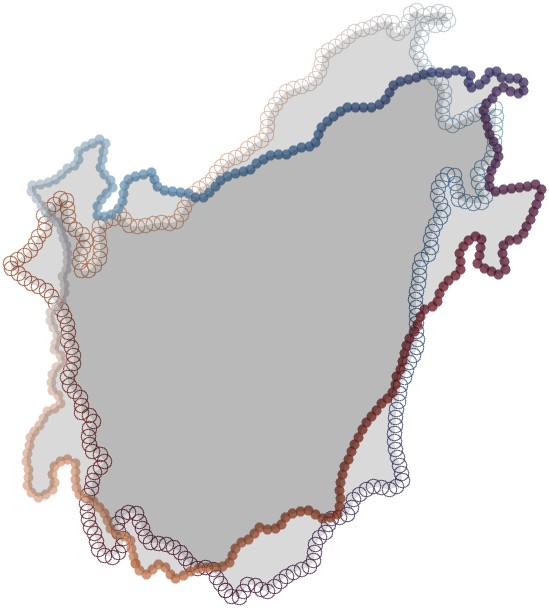
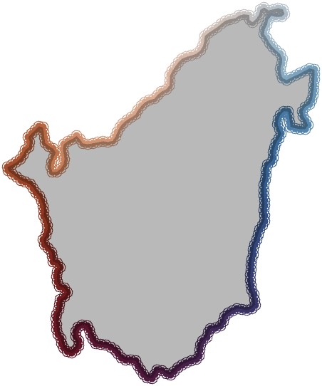
Figure 2: (left) An arbitrary cyclic permutation and rotation of a uniformly discrete grain shape with colors indicating row index with $n=250$. (center) An orthogonal Procrustes match. (right) A cyclic Procrustes match.

3.2 Functional Approximation

In this subsection, we revisit the assumption of sufficiently regular grain boundary interpolations to extend the discussion of Nyström method for curves in section 2.1 to obtain numerical approximations of (23)-(25) with spectral accuracy. We simplify to a $d\times d$ eigen-problem as opposed to the larger $n\times n$ problem in (21).

To begin, from (12.15) in [19], we have the SVD basis from the Nyström method written as

$$\bm{v}^{\top}(s)=\mathbb{k}^{\top}(s)WV\Sigma^{-2}_{d}$$ (32)

with

$$\mathbb{k}^{\top}(s) =(K(s,s_{1}),\cdots,K(s,s_{n}))$$

$$=\bm{o}^{\top}(s)\left(\begin{matrix}o_{1}(s_{1})&o_{1}(s_{2})&\cdots&o_{1}(s_{n})\\ \vdots&&&\\ o_{d}(s_{1})&o_{d}(s_{2})&\cdots&o_{d}(s_{n})\end{matrix}\right).$$

The expression $\bm{v}^{\top}(s)\coloneqq(v_{1},\dots,v_{d})(s)$ represents the $d$-tuple of evaluation functionals (23), as a row vector, approximated with a quadrature rule and collocated at $s$. Now, as in section 2.2, we will rewrite this expression without explicit dependence on the eigenvectors, $V$, on the right-hand side. Note that $K$ of (13) satisfies rank$(K)=d$ and, hence,

$$\bm{v}^{\top}(s)=\mathbb{k}^{\top}(s)W(\mathbb{v}_{1}/\sigma_{1}^{2},\mathbb{v}_{2}/\sigma_{2}^{2},\cdots,\mathbb{v}_{d}/\sigma_{d}^{2})$$

where $\mathbb{v}_{j}$, $j=1,\dots,d$, are the column vectors of $V$. Moreover, with a quadrature of $\bm{\alpha}_{j}$ as defined in the proof of Thm. 1,

$$\bm{\alpha}^{\top}_{j}\coloneqq(o_{1}^{\top}(\mathbb{s})W\mathbb{v}_{j},\cdots,o_{d}^{\top}(\mathbb{s})W\mathbb{v}_{j}),$$

utilizing the shorthand $o_{j}^{\top}(\mathbb{s})=(o_{j}(s_{1}),\dots,o_{j}(s_{n}))$ as a row vector of component function evaluations at quadrature nodes, we have

$$\bm{v}^{\top}(s)=\bm{o}^{\top}(s)(\bm{\alpha}_{1}/\sigma_{1}^{2},\bm{\alpha}_{2}/\sigma_{2}^{2},\cdots,\bm{\alpha}_{d}/\sigma_{d}^{2}).$$ (33)

Numerically, (33) is (23) in the context of the Nyström method. We now follow the approach of section 2.2 to obtain numerical approximations of (24) and (25). Let $\mathbb{s}\in\mathbb{R}^{n}$ be the vector of quadrature nodes and $\mathcal{A}=(\bm{\alpha}_{1},\bm{\alpha}_{2},\cdots,\bm{\alpha}_{d})\in\mathbb{O}(d)$ following the proof of Thm. 1, then

$$\bm{v}^{\top}(\mathbb{s})=(o_{1}(\mathbb{s}),\cdots,o_{d}(\mathbb{s}))\mathcal{A}\Sigma_{d}^{-2}$$

with $\Sigma_{d}^{-2}=\text{diag}(1/\sigma_{1}^{2},1/\sigma_{2}^{2},\dots,1/\sigma^{2}_{d})$ and

$$(o_{1}(\mathbb{s}),\cdots,o_{d}(\mathbb{s}))^{\top}W\bm{v}^{\top}(\mathbb{s})=\mathcal{A},$$

by definition of $\bm{\alpha}_{j}$. Thus, in place of (24) and taking $O_{n}=(o_{1}(\mathbb{s}),\cdots,o_{d}(\mathbb{s}))\in\mathbb{R}^{n\times d}_{*}$ as the matrix of (centered) curve evaluations at the $n$ quadrature nodes, we have $O_{n}^{\top}WO_{n}\mathcal{A}\Sigma_{d}^{-2}=\mathcal{A}$ which reveals the form of a weighted eigendecompostion,

$$O^{\top}_{n}WO_{n}=\mathcal{A}\Sigma^{2}_{d}\mathcal{A}^{\top}.$$ (34)

In short, $\bm{\alpha}_{j}$, $1\leq j\leq d$ as the columns of $\mathcal{A}$, are obtained simultaneously using an appropriate scheme to compute the weighted decomposition (34), instead of separately via (25), and (33) may be used to evaluate the eigenfunctions at any point $s$, if needed. However, notice we can simply utilize $V\coloneqq O_{n}\mathcal{A}\Sigma_{d}^{-1}\in\mathbb{R}^{n\times d}_{*}$ as the matrix of approximate eigenfunctions collocated at quadrature nodes representing discretizations of dual evaluation functionals.

However we must compute $\widetilde{V}$ and/or $\widetilde{X}$ with orthonormal columns for numerical implementations [30]. With each (centered) curve we can equivalently compute the thin weighted-SVD, or square-root quadrature decomposition, (SRQD)

$$O_{n}^{\top}W^{1/2}\,\overset{SVD}{=}\mathcal{A}\Sigma_{d}\widetilde{V}^{\top}$$ (35)

such that $\widetilde{X}\coloneqq\widetilde{V}\mathcal{A}^{\top}$, for all curves utilizing rapid decomposition schemes. The resulting right singular vectors $\widetilde{V}$ are the weighted eigenvectors, $\widetilde{V}=W^{1/2}V$, of (21) in the Nyström method. Thus, fast rank-$d$ SRQDs can efficiently map thousands of pre-shapes to discrete PRRTI-features. Equivalently, this fixed-order (spectral) numerical integration constitutes $\{O_{n}\}\mapsto\{(\widetilde{X},P)\}$ where $P\coloneqq\mathcal{A}\Sigma_{d}\mathcal{A}^{\top}$ are the separated scale variations in a weighted polar decomposition, $W^{1/2}O_{n}=\widetilde{X}P$.

Thus, the SRQD equivalently maps into separated pieces of generalized (anisotropic) scale variations $P\in S^{d}_{++}$, and representative orthonormal (pre-shape) undulations $\widetilde{X}$ of the Stiefel manifold, i.e., $\widetilde{X}^{\top}\widetilde{X}=\mathbb{I}_{d}$. Consequently, Thm. 1 motivates rapid and accurate weighted decompositions collocated at $n$ quadrature nodes instead of increasing sequences $(s_{i})_{i=1}^{n}$ from alternative reparametrizations or optimizations. We saturate accuracy in this approximation for all curves in the ensemble by by taking $n$ large, e.g., $n=500$.

3.3 Ensemble Manifold Learning

With a set of accurate discrete PRRTI-features $\{\widetilde{X}\}$ and corresponding scales $\{P\}$ from aggregated pairs of images, we briefly review an approach to learning an underlying (latent) space of features from thousands or tens of thousands of curves. Naturally, to retain the sought properties of Lemma 4 (PRRTI-features) and separation of generalized scale $P\in S^{d}_{++}\subset GL_{d}(\mathbb{R})$ in the representative Stiefel discretizations $\widetilde{V}$ and/or $\widetilde{X}$, we must project approximated eigenfunctions onto the equivalence classes $[\widetilde{V}]\in\mathbb{R}^{n\times d}_{*}/GL_{d}(\mathbb{R})$ constituting the shape of undulations. As described in [1], this quotient space is identified with the Grassmannian, $Gr(d,n)\cong\mathbb{R}^{n\times d}_{*}/GL_{d}(\mathbb{R})$. Note, $[\widetilde{V}]=[\widetilde{X}]$ but $\widetilde{X}$ serves as the representative pre-shape paired with scale variations $P$ in the polar decomposition. With $\{(\widetilde{X},P)\}$ as SRQD transformed data from a full ensemble given pairs of EBSD images, we leverage the tangent PCA submanifold learning procedure [30, 20], separately, over underlying matrix-manifolds $\{[\widetilde{X}]\}\subset Gr(d,n)$ and $\{P\}\subset S^{d}_{++}$. This procedure, with thousands of shapes, executes in seconds on a conventional modern laptop.

For example, tangent PCA proceeds with an ensemble of discrete matrix-valued PRRTI-features $\{[\widetilde{X}]\}$ first approximating the intrinsic/Karcher mean over $Gr(n,d)$, denoted $[\widetilde{V}_{0}]$. Interestingly, the Karcher mean visually appears to be predominantly circular over each pair of images—i.e., the hypothesis that a circle is a kind of ‘average’ archetypal grain shape is perhaps supported by this computation and reinforces our chosen alignment approach utilizing cyclic Procrustes. With the Karcher mean establishing a local origin for a coordinate frame, we apply PCA to the image of the inverse exponential at $[\widetilde{V}_{0}]$ to determine normal coordinates, $\bm{t}\in\mathbb{R}^{r}$, over an $r$-dimensional subspace, $1\leq r\leq d(n-d)$. The span of this subspace parametrizes undulations over the matrix-manifold as a local section $\mathcal{G}_{r}\subseteq Gr(d,n)$, i.e.,

$$\mathcal{G}_{r}\coloneqq\{[X]\in Gr(d,n)\,:\,[X]=\text{Exp}_{[\widetilde{V}_{0}]}(T_{r}\bm{t})\},$$ (36)

where $T_{r}$ is the ‘learned’ matrix with columns constituting an ordered orthonormal basis of $\mathbb{R}^{r}\cong T_{[\widetilde{V}_{0}]}\mathcal{G}_{r}$. This same learning procedure is repeated, separately, with $\{P\}$ to determine the intrinsic mean $P_{0}\in\mathcal{P}\subseteq S^{d}_{++}$ and tangent basis spanning $T_{P_{0}}\mathcal{P}\subseteq T_{P_{0}}S^{d}_{++}$ facilitated by the algorithms in [21]. In our materials application, $\mathcal{P}$ is taken to be all of $S^{d}_{++}$ but other applications may benefit from coordiantes along subspaces of $T_{P_{0}}S^{d}_{++}$. Finally, consistent with [30], we utilize $\mathcal{G}_{r}\times\mathcal{P}$ as a product submanifold of separable (pre-)shape tensors parametrized with smooth right inverse $O_{n}(\bm{t},\bm{\ell})=\widetilde{X}(\bm{t})P(\bm{\ell})$ over normal coordinates $(\bm{t},\bm{\ell})\in T_{[\widetilde{V}_{0}]}\mathcal{G}_{r}\times T_{P_{0}}\mathcal{P}$.

Changing dimensionality $r$ by accumulating terms in the ordered basis expansion over normal coordinates, $\bm{t}\in\mathbb{R}^{r}\cong T_{[\widetilde{V}_{0}]}\mathcal{G}_{r}$, can empirically achieve the sought regularization of (1) in the representation of the shapes. This observed mechanism can promote a biasing of undulating shape features away from potentially noisy variations in the segmented grain boundaries. An example of the empirical effects of this regularization are shown in Figure 3. We anticipate that this choice of undulation dimensionality can be used to make subsequent inferences more robust against noisy measurements and image processing.

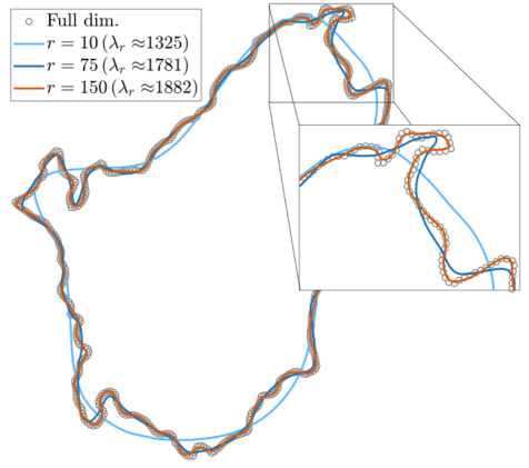
Figure 3: The empirical effect of the sought shape regularization (1) over changing submanifold dimensionality, $r$, with $n=500$ landmarks from a reparametrized spline. Lipschitz constants of the curves are approximated using chebfun, an open source toolbox being utilized to compute quasi-matrix interpolation (28) of the reduced dimension analogs.

3.4 Maximum Mean Discrepancy (MMD)

Having formalized the spectral approximation of curve dual evaluation functionals with (shape) discretizations parametrized over the Grassmannian, we explore an explainable binary classification of the learned undulation and scale coordinates $(\bm{t},\bm{\ell})\in T_{[\widetilde{V}_{0}]}\mathcal{G}_{r}\times T_{P_{0}}\mathcal{P}$ defined at respective intrinsic means $[\widetilde{V}_{0}]\in\mathcal{G}_{r}\subseteq Gr(n,d)$ and $P_{0}\in\mathcal{P}\subseteq S^{d}_{++}$. We require all the furnishings of a Borel $\sigma$-algebra for $(\bm{t},\bm{\ell})\in T_{[\widetilde{V}_{0}]}\mathcal{G}_{r}\times T_{P_{0}}\mathcal{P}$ in a normal coordinate neighborhood assumed to be restricted to some geodesic ball constituting a metric space—i.e., Hopf-Rinow theorem. Thus, we take $(\bm{t},\bm{\ell})\sim\bm{\rho}$ as some joint distribution given by the smallest $\sigma$-finite (product) measure of random shape (normal) coordinates generated by the metric spaces.

Given ensembles of segmented curves as data, if separable parameters are assumed independent, $\bm{\rho}=\rho_{\bm{t}}\rho_{\bm{\ell}}$, we demonstrate that separate hypothesis tests over $\bm{t}$ and $\bm{\ell}$ offer a logical test as explanation by the product maximum mean discrepancy (pMMD). These results are bolstered by numerical examples depicted and described in Figures 4-7 emphasizing each row of the logical conjunction Truth Table 1.

Case	$(\rho_{\bm{t}}=\widehat{\rho}_{\bm{t}})$	$(\rho_{\bm{\ell}}=\widehat{\rho}_{\bm{\ell}})$	$\text{pMMD}[\mathcal{H}\oplus\mathcal{Q},\cdot,\cdot]$
$(1\wedge 1)$	Accept	Accept	$\implies$ Accept
$(1\wedge 0)$	Accept	Reject	$\implies$ Reject
$(0\wedge 1)$	Reject	Accept	$\implies$ Reject
$(0\wedge 0)$	Reject	Reject	$\implies$ Reject

Table 1: A logical conjunction (AND gate) for the two separable hypothesis tests (left of the double vertical lines) using pMMD. In keeping with the definition of ‘truth’ in a hypothesis test, ‘acceptance’ of the null hypothesis is considered as a logical ‘true’ condition. This definition of ’truth’ is color-coded red in the table.

The goal of MMD [22, 27] is to determine if finite observations of independent and identically distributed (i.i.d.) random variables defined on a topological space, with respective probability measures, coincide or not. That is, for joint measures $\bm{\rho}$ and $\widehat{\bm{\rho}}$, given observations $\{\bm{\theta}_{1},\dots,\bm{\theta}_{N}\}$ and $\{\widehat{\bm{\theta}}_{1},\dots,\widehat{\bm{\theta}}_{\widehat{N}}\}$ assumed i.i.d. from $\bm{\rho}$ and $\widehat{\bm{\rho}}$ respectively, can we test whether $\bm{\rho}\neq\widehat{\bm{\rho}}$? With separable parameters, in a complementary fashion, can we test whether $(\rho_{\bm{t}}=\widehat{\rho}_{\bm{t}})$ and $(\rho_{\bm{\ell}}=\widehat{\rho}_{\bm{\ell}})$? This formal problem statement is the quantitative analog of the proposed explainable binary classification: test if the ensemble of random shape coordinates between two images are discrepant, ignoring rigid motions, and whether those discrepancies result from distinct distributions over undulation or scale. This separable formalism is simply De Morgan’s theorem, $(\rho_{\bm{t}}=\widehat{\rho}_{\bm{t}})\wedge(\rho_{\bm{\ell}}=\widehat{\rho}_{\bm{\ell}})\leftrightarrow\neg((\rho_{\bm{t}}\neq\widehat{\rho}_{\bm{t}})\vee(\rho_{\bm{\ell}}\neq\widehat{\rho}_{\bm{\ell}}))$. Truth Table 1 details this formalism where logical truth corresponds to accepting the null hypothesis, $(\rho_{\cdot}=\widehat{\rho}_{\cdot})$, in comparison and thresholds set for the various hypotheses tests are discussed in [27].

To elaborate on the precise logical implications, we follow the development of [27] and utilize MMD defined over a unit ball in a RKHS, $\mathcal{F}$, as

$$\text{MMD}[\mathcal{F},\bm{\rho},\widehat{\bm{\rho}}\,]\coloneqq\sup_{\psi\in\mathcal{F}}|\mathbb{E}_{\bm{\theta}\sim\bm{\rho}}[\psi(\bm{\theta})]-\mathbb{E}_{\widehat{\bm{\theta}}\sim\widehat{\bm{\rho}}}[\psi(\widehat{\bm{\theta}}\,)]|.$$ (37)

We note that this RKHS is, presently, distinct from the $\mathbb{R}^{d}$-valued RKHSs motivated by Thm. 1. Instead, $\mathcal{F}$ is an RKHS representing features of ‘learned’ parameter distributions informed by the tangent PCA of generalized scale and discrete undulations. Here, $\mathbb{E}_{(\cdot)}$ represents expectation (integration) with respect to the identified probability measures over some arbitrary tuple of parameters, $\bm{\theta},\widehat{\bm{\theta}}\in\Theta\subseteq\mathbb{R}^{r+3}$, from distinct measurements distinguished as $\bm{\theta}$ versus $\widehat{\bm{\theta}}$. Solutions to (37) are motivated empirically utilizing a choice of symmetric positive definite kernel, $f:\Theta\times\Theta\rightarrow\mathbb{R}:(\bm{\theta},\widehat{\bm{\theta}}\,)\mapsto f(\bm{\theta},\widehat{\bm{\theta}}\,)$, and Lemma 6 in [27] such that we can express the squared population MMD over $\mathcal{F}$ as

$$\text{MMD}^{2}[\mathcal{F},\bm{\rho},\widehat{\bm{\rho}}\,]=\bm{E}_{\bm{\rho}}[f]+\bm{E}_{\widehat{\bm{\rho}}}[f]-2\bm{E}_{\bm{\rho}\widehat{\bm{\rho}}}[f].$$ (38)

This rewrite utilizes a simplification via the ‘tower property’ such that $\bm{E}_{\bm{\rho}}[f]\coloneqq{\mathbb{E}}_{\bm{\rho}}[\,{\mathbb{E}}_{\bm{\rho}}[f|\bm{\theta}]\,]$ is a double expectation over $\bm{\rho}$, similarly for $\bm{E}_{\widehat{\bm{\rho}}}$, and $\bm{E}_{\bm{\rho}\widehat{\bm{\rho}}}\coloneqq\mathbb{E}_{\bm{\rho}}[\,\mathbb{E}_{\widehat{\bm{\rho}}}[f|\bm{\theta}]\,]$ is a double expectation over both and in that order. Additionally, as a shorthand we denote ${\mathbb{E}}_{\bm{t}}[\cdot]\coloneqq{\mathbb{E}}_{\rho_{\bm{t}}}[\cdot]$ and $\widehat{{\mathbb{E}}}_{\bm{t}}[\cdot]\coloneqq{\mathbb{E}}_{\,\widehat{\rho}_{\bm{t}}}[\cdot]$, similarly over $\bm{\ell}\sim\rho_{\bm{\ell}}$ and $\widehat{\bm{\ell}}\sim\widehat{\rho}_{\bm{\ell}}$, to more clearly indicate parameter dependencies.

Lemma 6 (Commutativity by Tonelli-Fubini, [38]).

With a positive measurable function or integrable function $f$, i.e., both sections $\bm{\theta}\mapsto f(\bm{\theta},\cdot)$ and $\bm{\theta}\mapsto f(\cdot,\bm{\theta})$ measurable, then

$$\bm{E}_{\bm{\rho}\widehat{\bm{\rho}}}[f]=\bm{E}_{\widehat{\bm{\rho}}\bm{\rho}}[f].$$

Proof.

By Tonelli-Fubini theorem of Lebesgue integrable functions, Thm. 10.3 [38]. ∎

Following the presentation of [27], we take a separable kernel $f:\Theta\times\Theta\rightarrow\mathbb{R}$ by the direct product of RKHSs, $\mathcal{F}\coloneqq\mathcal{H}\oplus\mathcal{Q}$, over $T_{[\widetilde{V}_{0}]}\mathcal{G}_{r}$ and $T_{P_{0}}\mathcal{P}$, i.e.

$$f((\bm{t},\bm{\ell}),(\cdot,\cdot))=h(\bm{t},\cdot)q(\bm{\ell},\cdot),$$ (39)

with kernels $h:T_{[\widetilde{V}_{0}]}\mathcal{G}_{r}\times T_{[\widetilde{V}_{0}]}\mathcal{G}_{r}\rightarrow\mathbb{R}$ and $q:T_{P_{0}}\mathcal{P}\times T_{P_{0}}\mathcal{P}\rightarrow\mathbb{R}$.

Lemma 7 (Separable Canonical Feature Maps).

If $\bm{t}\sim\rho_{\bm{t}}$ and $\bm{\ell}\sim\rho_{\bm{\ell}}$ are independent, then the mean embedding $\varphi\in\mathcal{H}\oplus\mathcal{Q}$ of the distribution $\bm{\rho}$ such that

$${\mathbb{E}}_{\bm{\rho}}[g]=\langle g,\varphi\rangle_{\mathcal{F}}$$

for all $g\in\mathcal{F}$, admits a separable canonical feature map,

$$\varphi(\bm{t},\bm{\ell})=\varphi_{h}(\bm{t})\varphi_{q}(\bm{\ell}).$$

Equivalently, $\bm{E}_{\bm{\rho}}[hq]={\mathbb{E}}_{\bm{\rho}}[\varphi_{h}\varphi_{q}]={\mathbb{E}}_{\bm{t}}[\varphi_{h}]{\mathbb{E}}_{\bm{\ell}}[\varphi_{q}].$

Proof.

Following the proof and definitions in Lemma 3 and Theorem 5 of [27], beginning with Riesz’s representer theorem followed by the definition of the mean embedding,

$$\varphi(\bm{t},\bm{\ell}) =\langle\varphi,f((\bm{t},\bm{\ell}),(\cdot,\cdot))\rangle_{\mathcal{F}}$$

$$=\mathbb{E}_{\bm{\rho}}[f\,|\,(\bm{t},\bm{\ell})]$$

(separable) $$=\mathbb{E}_{\bm{\rho}}[hq\,|\,(\bm{t},\bm{\ell})]$$

(independent) $$={\mathbb{E}}_{\bm{t}}[h\,|\,\bm{t}]{\mathbb{E}}_{\bm{\ell}}[q\,|\,\bm{\ell}]$$

(Doob-Dynkin lemma) $$=\varphi_{h}(\bm{t})\varphi_{q}(\bm{\ell}).$$

∎

Next, we demonstrate how the canonical MMD defined over the joint distributions, $\text{MMD}[\mathcal{F},\bm{\rho},\widehat{\bm{\rho}}\,]$, constitutes an almost logical conjunction where ‘truth’ is defined as equality in the assumed independent distributions over $\bm{t}$ and $\bm{\ell}$.

Lemma 8 (An Almost Logical Conjunction).

Given a separable kernel $v:\Theta\times\Theta\rightarrow\mathbb{R}$ and assuming independent parameters $\bm{t}\in T_{[\widetilde{V}_{0}]}\mathcal{G}_{r}$ and $\bm{\ell}\in T_{P_{0}}\mathcal{P}$,

• Case 1, row 1 Table 1: if $\rho_{\bm{t}}=\widehat{\rho}_{\bm{t}}$ and $\rho_{\bm{\ell}}=\widehat{\rho}_{\bm{\ell}}$ then

  $$\text{MMD}[\mathcal{F},\bm{\rho},\widehat{\bm{\rho}}\,]=0.$$

• Case 2, rows 2-3 Table 1: if either $\rho_{\bm{t}}=\widehat{\rho}_{\bm{t}}$ or $\rho_{\bm{\ell}}=\widehat{\rho}_{\bm{\ell}}$ and not the other, i.e., exclusively such that one distribution of parameters is equal while the other distributions are not, then

  $$\text{MMD}^{2}[\mathcal{F},\bm{\rho},\widehat{\bm{\rho}}\,]>0.$$

Proof.

We start by demonstrating Case 2 which subsequently simplifies to Case 1. Factoring the separable and independent form of $\text{MMD}^{2}[\mathcal{F},\bm{\rho},\widehat{\bm{\rho}}\,]$ by Lemmas 6 and 7,

$$\text{MMD}^{2}[\mathcal{F},\bm{\rho},\widehat{\bm{\rho}}\,] =\bm{E}_{\bm{\rho}}[f]+\bm{E}_{\widehat{\bm{\rho}}}[f]-2\bm{E}_{\bm{\rho}\widehat{\bm{\rho}}}[f]$$

$$(\text{separability}) =\bm{E}_{\bm{\rho}}[hq]+\bm{E}_{\widehat{\bm{\rho}}}[hq]-2\bm{E}_{\bm{\rho}\widehat{\bm{\rho}}}[hq]$$

$$(\text{Lemma}~{}\ref{lemma:tonelli}) =(\bm{E}_{\bm{\rho}}[hq]-\bm{E}_{\bm{\rho}\widehat{\bm{\rho}}}[hq])$$

$$\quad+(\bm{E}_{\widehat{\bm{\rho}}}[hq]-\bm{E}_{\widehat{\bm{\rho}}\bm{\rho}}[hq])$$

$$(\text{Lemma}~{}\ref{lemma:sep_features}) =({\mathbb{E}}_{\bm{t}}[\varphi_{h}]{\mathbb{E}}_{\bm{\ell}}[\varphi_{q}]-{\mathbb{E}}_{\bm{t}}[\widehat{\varphi}_{h}]{\mathbb{E}}_{\bm{\ell}}[\widehat{\varphi}_{q}])$$

$$\quad+(\widehat{{\mathbb{E}}}_{\bm{t}}[\widehat{\varphi}_{h}]\widehat{{\mathbb{E}}}_{\bm{\ell}}[\widehat{\varphi}_{q}]-\widehat{{\mathbb{E}}}_{\bm{t}}[\varphi_{h}]\widehat{{\mathbb{E}}}_{\bm{\ell}}[\varphi_{q}]).$$

Consequently, following the proof of Theorem 5 in [27], if $\rho_{\bm{t}}=\widehat{\rho}_{\bm{t}}$ then $\varphi_{h}=\widehat{\varphi}_{h}$, i.e., injective feature embeddings, and

$$E={\mathbb{E}}_{\bm{t}}[\varphi_{h}]={\mathbb{E}}_{\bm{t}}[\widehat{\varphi}_{h}]=\widehat{{\mathbb{E}}}_{\bm{t}}[\widehat{\varphi}_{h}]=\widehat{{\mathbb{E}}}_{\bm{t}}[\varphi_{h}]$$

is some constant by Lemma 1 of [27]. Thus, factoring the constant,

$$\text{MMD}^{2}[\mathcal{F},\bm{\rho},\widehat{\bm{\rho}}\,] \propto({\mathbb{E}}_{\bm{\ell}}[\varphi_{q}]-{\mathbb{E}}_{\bm{\ell}}[\widehat{\varphi}_{q}])+(\widehat{{\mathbb{E}}}_{\bm{\ell}}[\widehat{\varphi}_{q}]-\widehat{{\mathbb{E}}}_{\bm{\ell}}[\varphi_{q}])$$

$$=\bm{E}_{\bm{\rho}}[q]+\bm{E}_{\widehat{\bm{\rho}}}[q]-2\bm{E}_{\bm{\rho}\widehat{\bm{\rho}}}[q]$$

$$=\text{MMD}^{2}[\mathcal{Q},\rho_{\bm{\ell}},\widehat{\rho}_{\bm{\ell}}].$$

Similarly when $\rho_{\bm{\ell}}=\widehat{\rho}_{\bm{\ell}}$,

$$\text{MMD}^{2}[\mathcal{F},\bm{\rho},\widehat{\bm{\rho}}\,]\propto\text{MMD}^{2}[\mathcal{H},\rho_{\bm{t}},\widehat{\rho}_{\bm{t}}].$$

Therefore, the larger problem factors into separate tests of MMD over separable and independent parameters. That is, if either ($\rho_{\bm{t}}=\widehat{\rho}_{\bm{t}}$ and $\rho_{\bm{\ell}}\neq\widehat{\rho}_{\bm{\ell}}$) or ($\rho_{\bm{t}}\neq\widehat{\rho}_{\bm{t}}$ and $\rho_{\bm{\ell}}=\widehat{\rho}_{\bm{\ell}}$), i.e., exclusively, then

$$\text{MMD}^{2}[\mathcal{F},\bm{\rho},\widehat{\bm{\rho}}\,]>0.$$

Of course, if $\rho_{\bm{t}}=\widehat{\rho}_{\bm{t}}$ and $\rho_{\bm{\ell}}=\widehat{\rho}_{\bm{\ell}}$, then

$$\text{MMD}^{2}[\mathcal{F},\bm{\rho},\widehat{\bm{\rho}}\,]=0,$$

i.e., $E\cdot 0=0$. ∎

However, the ‘distance’ $\text{MMD}[\mathcal{F},\rho_{\bm{t}}\rho_{\bm{\ell}},\widehat{\rho}_{\bm{t}}\widehat{\rho}_{\bm{\ell}}]$ comparing joint distributions as products of the pairs independent distributions, $(\rho_{\bm{t}},\rho_{\bm{\ell}})\mapsto\rho_{\bm{t}}\rho_{\bm{\ell}}$, can vanish over the direct product of RKHSs:

Theorem 2 (Vanishing MMD).

Given a separable kernel $f:\Theta\times\Theta\rightarrow\mathbb{R}$ and assuming independent parameters $\bm{t}\in T_{[\widetilde{V}_{0}]}\mathcal{G}_{r}$ and $\bm{\ell}\in T_{P_{0}}\mathcal{P}$, MMD over the direct product of RKHSs admits a vanishing distance over the Cartesian product of densities.

Proof.

Intuitively, given $(\rho_{\bm{t}},\rho_{\bm{\ell}})$ and $(\widehat{\rho}_{\bm{t}},\widehat{\rho}_{\bm{\ell}})$ one might hope $\rho_{\bm{t}}\neq\widehat{\rho}_{\bm{t}}$ and $\rho_{\bm{\ell}}\neq\widehat{\rho}_{\bm{\ell}}$ would necessarily bound the metric, $\text{MMD}[\mathcal{F},\bm{\rho},\widehat{\bm{\rho}}\,]$, away from zero. However, consider the rather simple counterexample such that $\text{MMD}^{2}[\mathcal{F},\bm{\rho},\widehat{\bm{\rho}}\,]=0$ if and only if $\varphi=\widehat{\varphi}$ [27]. Consequently, by Lemma 7, $\varphi_{h}\varphi_{q}=\widehat{\varphi}_{h}\widehat{\varphi}_{q}$ implies

$$\varphi_{h}/\widehat{\varphi}_{q}=\widehat{\varphi}_{h}/\varphi_{q}$$

when both sides of either expression are defined over their support. Setting both sides equal to a constant implies $\varphi_{h}=C\widehat{\varphi}_{q}$ and $\widehat{\varphi}_{h}=C\varphi_{q}$ if and only if $\text{MMD}^{2}[\mathcal{H}\oplus\mathcal{Q},\bm{\rho},\widehat{\bm{\rho}}\,]=0$ with some choice of reproducing kernels. This can be generalized in our notation as

$$\text{MMD}^{2}[\mathcal{F},\bm{\rho},\widehat{\bm{\rho}}\,] =\bm{E}_{\bm{\rho}}[f]+\bm{E}_{\widehat{\bm{\rho}}}[f]-2\bm{E}_{\bm{\rho}\widehat{\bm{\rho}}}[f]$$

$$(\text{Lemma}~{}\ref{lemma:tonelli}) =(\bm{E}_{\bm{\rho}}[hq]-\bm{E}_{\bm{\rho}\widehat{\bm{\rho}}}[hq])$$

$$\quad+(\bm{E}_{\widehat{\bm{\rho}}}[hq]-\bm{E}_{\widehat{\bm{\rho}}\bm{\rho}}[hq])$$

$$(\text{Lemma}~{}\ref{lemma:sep_features}) =({\mathbb{E}}_{\bm{\rho}}[\varphi_{h}\varphi_{q}]-{\mathbb{E}}_{\bm{\rho}}[\widehat{\varphi}_{h}\widehat{\varphi}_{q}])$$

$$\quad+({\mathbb{E}}_{\,\widehat{\bm{\rho}}}[\widehat{\varphi}_{h}\widehat{\varphi}_{q}]-{\mathbb{E}}_{\,\widehat{\bm{\rho}}}[\varphi_{h}\varphi_{q}])$$

$$(\text{linearity}) ={\mathbb{E}}_{\bm{\rho}}[\varphi_{h}\varphi_{q}-\widehat{\varphi}_{h}\widehat{\varphi}_{q}]$$

$$\quad+{\mathbb{E}}_{\,\widehat{\bm{\rho}}}[\widehat{\varphi}_{h}\widehat{\varphi}_{q}-\varphi_{h}\varphi_{q}]$$

which is evidently zero when $\varphi_{1}={\mathbb{E}}_{\bm{t}}[h\,|\,\bm{t}]=C\widehat{{\mathbb{E}}}_{\bm{\ell}}[q\,|\,\bm{\ell}]$ and $\varphi_{2}=\widehat{{\mathbb{E}}}_{\bm{t}}[h\,|\,\bm{t}]=C{\mathbb{E}}_{\bm{\ell}}[q\,|\,\bm{\ell}]$ are common canonical feature maps. For example, setting $C=1$, we may have $\rho_{\bm{t}}$ and $\widehat{\rho}_{\bm{\ell}}$ as zero mean Gaussian distributions, $\widehat{\rho}_{\bm{t}}$ and $\rho_{\bm{\ell}}$ common non-zero mean Gaussian distributions, and $h$ and $q$ common forms of kernels over separable parameters. Thus, $\rho_{\bm{t}}\neq\widehat{\rho}_{\bm{t}}$ and $\rho_{\bm{\ell}}\neq\widehat{\rho}_{\bm{\ell}}$ exhibit common, arbitrarily large, discrepancies in expectation but ${\mathbb{E}}_{\bm{\rho}}[\varphi_{1}\varphi_{2}-\varphi_{2}\varphi_{1}]={\mathbb{E}}_{\,\widehat{\bm{\rho}}}[\varphi_{2}\varphi_{1}-\varphi_{1}\varphi_{2}]=\mathbb{E}_{(\cdot)}[0]=0$. ∎

It is important to note that this distance does not vanish identically and is merely a special case of a relation satisfied by the separable and independent mean embeddings. However, an alternative product metric by any $p$-norm of pairs of separate MMD metrics,

$$\text{pMMD}[\mathcal{H}\oplus\mathcal{Q},(\rho_{\bm{t}},\rho_{\bm{\ell}}),(\widehat{\rho}_{\bm{t}},\widehat{\rho}_{\bm{\ell}})]\coloneqq\\ \biggl{\|}\left(\begin{matrix}\text{MMD}[\mathcal{H},\rho_{\bm{t}},\widehat{\rho}_{\bm{t}}]\\ \text{MMD}[\mathcal{Q},\rho_{\bm{\ell}},\widehat{\rho}_{\bm{\ell}}]\end{matrix}\right)\biggl{\|}_{p},$$ (40)

clearly satisfies the logical implication depicted in the Truth Table 1; specifically the last row such that $\rho_{\bm{t}}\neq\widehat{\rho}_{\bm{t}}$ and $\rho_{\bm{\ell}}\neq\widehat{\rho}_{\bm{\ell}}$ implies $\text{pMMD}[\mathcal{H}\oplus\mathcal{Q},(\rho_{\bm{t}},\rho_{\bm{\ell}}),(\widehat{\rho}_{\bm{t}},\widehat{\rho}_{\bm{\ell}})]>0$. Moreover, the use of the product metric is a somewhat natural choice by virtue of the product submanifold construction for the space of separable shape tensors.

4 Experiments

Descriptions and results of numerical experiments are depicted and explained in Figures 4-7. The combined numerical experiments enable explainable binary classifications of ice data [17, 18] and TRIP780 steel data measured at the National Institute of Standards and Technology (NIST) Material Measurement Laboratory (MML), which span Truth Table 1. The pre-processing of EBSD data to extract sorted vertices of grain boundaries is accomplished with the open-source toolbox MTEX [33]. All of the depicted numerical experiments utilize an undulation dimensionality of $r=150$—see Figure 3 for a representative approximation with this dimensionality—and three (full) dimensions of scale. The filled colors of the grain shapes in Figures 4-7 represent a normalized shape distance over the product submanifold measured from the approximate intrinsic mean shape.

Our numerical experiments emphasize four scenarios where these tools deliver benefits to materials scientists and practitioners investigating micrographs with EBSD:

• Figure 4, the method is not suspected to be overly sensitive to statistical rejection: we identified data which concluded, empirically, that there were no useful statistical discrepancies in the compared images.

• Figure 5, the method emulates conclusions consistent with human observations: when provided with data which has very clear human recognizable distinctions described as ‘scale variations,’ our method detects statistical differences in the measured shapes and results in a theoretical interpretation that scale is the significant factor.

• Figure 6, the method detects differences below human-scale visual observations: given an image processing routine that smooths an EBSD image differently, we demonstrate how the approach detects nonlinear variations in shapes which would otherwise go overlooked by cursory human inspection.

• Figure 7, the method detects a presumed faulty measurement: when provided with data which was suspected to be ‘out-of-focus’ utilizing the state-of-the-art measurement instrumentation, we were able to detect significant differences to indicate the presence of a problem.

5 Conclusion

In summary, we have established a formal interpretation between separable shape tensors (SST) and dual evaluation functionals of [44]. We demonstrate that spectral methods, based on an interpretation with the Nystöm method, can be utilized to offer highly accurate approximations of SSTs provided sufficient smoothness. We then elaborate on the alignment of SSTs and caveats of utilizing a maximum mean discrepancy (MMD) analysis to inform explainable binary classification of data. Finally, we highlight four numerical examples spanning the logical Truth Table 1 found in real EBSD measurements; identified by simple observations (selected for qualitative appearance), differences in pre-processing (smoothing), and detection of a presumed measurement issue (instrument out-of-focus).

Future work will expound on the identified relationships between finite matrix manifold representations of shape and the formal interpretations of infinite dimensional analogs detailed in [44]. In short, our efforts will be focused towards: i) formalizing bounds on the approximation error of reduced dimension SSTs, and ii) infinite dimensional extensions of pMMD explainable binary classifications over the $\mathbb{R}^{d}$-valued RKHSs of [44]. We also hope to improve explanations in the classification problem to understand which patterns of shape, in more detail, contribute to approximated discrepancies.

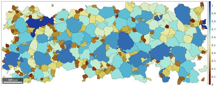
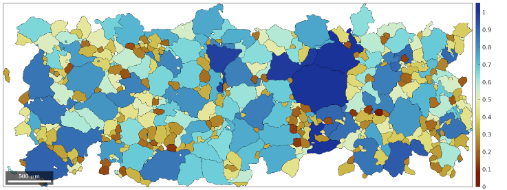
Figure 4: (Example $1\wedge 1$) Comparison of locally partitioned subsets of a larger EBSD images from a common ice sample [17] (PIL184) with $N=933$ total curves and $n=500$ landmarks per curve. No shapes or boundaries are duplicated between the partition. The approximate inferences suggest the same undulations and same scales. This constitutes an example of the first row of Truth Table 1, i.e., $1\wedge 1$.

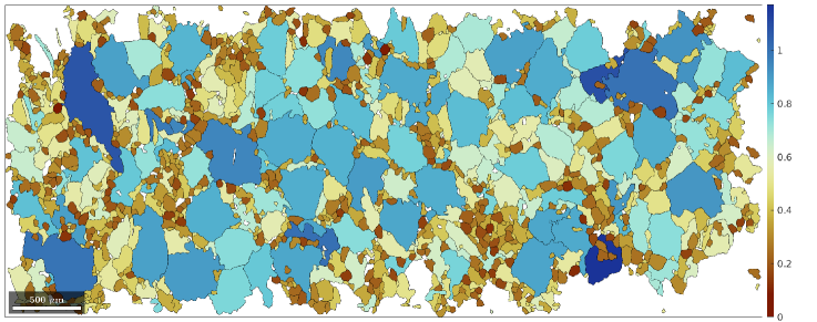
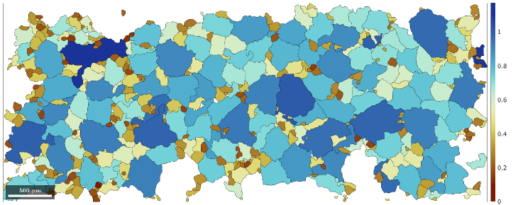
Figure 5: (Example $1\wedge 0$) Comparison of two different EBSD images of ice samples [17] (PIL185 and PIL184) with $N=2566$ curves in total and $n=500$ landmarks per curve. Both images depict cropped shape selections. (there are additional shapes beyond the selection depicted in the images) The approximate inferences suggest the same undulations but different scales between the two images. This constitutes an example of the second row of Truth Table 1, i.e., $1\wedge 0$.

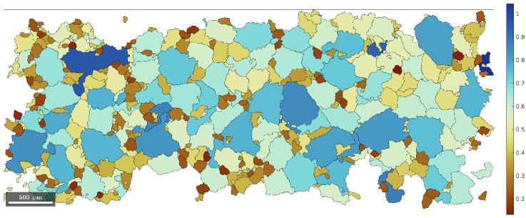
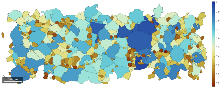
Figure 6: (Example $0\wedge 1$) Comparison of locally partitioned subsets of a larger EBSD images from a common ice sample [17] (PIL184) with $N=933$ total curves and $n=500$ landmarks per curve. No shapes or boundaries are duplicated between the partition and this partition is consistent with that of Figure 4. However, using a simple moving average in the MTEX ‘smooth’ routine [5], the upper partition (top image) is not smoothed while the bottom is smoothed to some extent ($31$ points in the ‘span’ of the smoothing). Magnifying and contrasting the top image with the bottom image of Figure 5 it is possible to see small differences in the nonlinearities of shapes. The difference is nearly visually indistinguishable. Yet, the approximate inferences suggest differences in undulations and common scales. This constitutes an example of the third row of Truth Table 1, i.e., $0\wedge 1$.

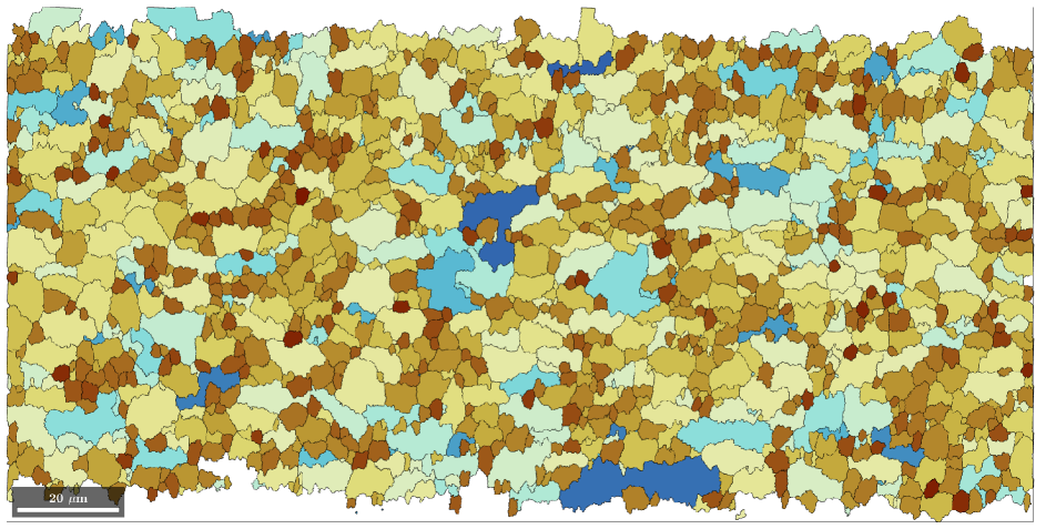
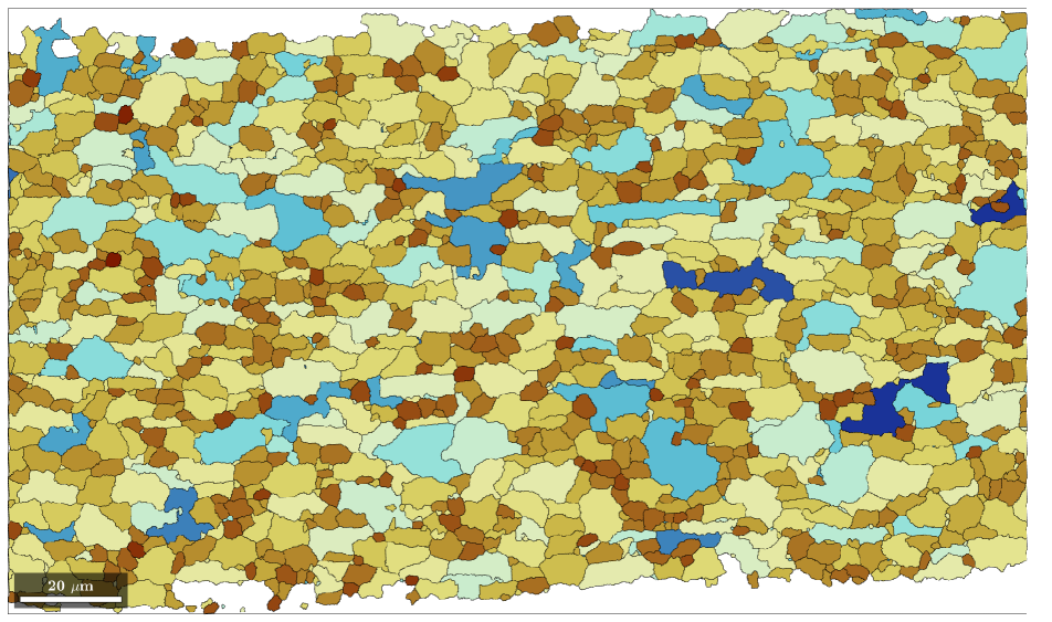
Figure 7: (Example $0\wedge 0$) Comparison of two different EBSD images of TRIP780 steel samples with $N=5605$ curves in total and $n=500$ interpolated landmarks per curve. Both images depict cropped shape selections to place emphasis on small scale features of undulation. (there are additional shapes beyond the depiction) The approximate inferences suggest differences in both undulations and scales between the two images. This constitutes an example of the last (fourth) row of Truth Table 1, i.e., $0\wedge 0$. Note, the hypothesis from a NIST materials scientist, Adam Creuziger, is that the upper sample was collected from a measurement which was ‘out-of-focus.’

References

- Absil et al. [2008] P.-A. Absil, R. Mahony, and R. Sepulchre. Optimization Algorithms on Matrix Manifolds. Princeton University Press, 2008.
- Al-Aifari et al. [2013] Reema Al-Aifari, Ingrid Daubechies, and Yaron Lipman. Continuous procrustes distance between two surfaces. Communications on Pure and Applied Mathematics, 66(6):934–964, 2013.
- Atindama et al. [2023] Emmanuel Atindama, Peter Lef, Günay Doğan, and Prashant Athavale. Restoration of noisy orientation maps from electron backscatter diffraction imaging. Integrating Materials and Manufacturing Innovation, 12(3):251–266, 2023.
- Bachmann et al. [2010a] Florian Bachmann, Ralf Hielscher, Peter E Jupp, Wolfgang Pantleon, Helmut Schaeben, and Elias Wegert. Inferential statistics of electron backscatter diffraction data from within individual crystalline grains. Journal of Applied Crystallography, 43(6):1338–1355, 2010a.
- Bachmann et al. [2010b] F Bachmann, Ralf Hielscher, and Helmut Schaeben. Texture analysis with MTEX–free and open source software toolbox. Solid state phenomena, 160:63–68, 2010b.
- Bachmann et al. [2011] Florian Bachmann, Ralf Hielscher, and Helmut Schaeben. Grain detection from 2d and 3d ebsd data—specification of the mtex algorithm. Ultramicroscopy, 111(12):1720–1733, 2011.
- Bauer et al. [2014] Martin Bauer, Martins Bruveris, and Peter W Michor. Overview of the geometries of shape spaces and diffeomorphism groups. Journal of Mathematical Imaging and Vision, 50:60–97, 2014.
- Bendokat et al. [2020] Thomas Bendokat, Ralf Zimmermann, and P-A Absil. A Grassmann manifold handbook: Basic geometry and computational aspects. arXiv preprint arXiv:2011.13699, 2020.
- Bruveris [2016] Martins Bruveris. Optimal reparametrizations in the square root velocity framework. SIAM Journal on Mathematical Analysis, 48(6):4335–4354, 2016.
- Bryner et al. [2014] D. Bryner, E. Klassen, H. Le, and A. Srivastava. 2D affine and projective shape analysis. IEEE Transactions on Pattern Analysis and Machine Intelligence, 36(5):998–1011, 2014.
- Constantine and Phipps [2012] Paul G Constantine and Eric T Phipps. A lanczos method for approximating composite functions. Applied Mathematics and Computation, 218(24):11751–11762, 2012.
- De Marchi and Santin [2013] S. De Marchi and S. Santin. A new stable basis for radial basis function interpolation. 253:1–13, 2013.
- Doronina et al. [2023] Olga A. Doronina, Zachary J. Grey, and Andrew Glaws. G2aero: A python package for separable shape tensors. Journal of Open Source Software, 8(89):5408, 2023.
- Doğan et al. [2015] Günay Doğan, Javier Bernal, and C Hagwood. FFT-based alignment of 2d closed curves with application to elastic shape analysis. In DIFF-CV, British Machine Vision Conference (BMVC), 2015.
- Durrleman et al. [2014] Stanley Durrleman, Marcel Prastawa, Nicolas Charon, Julie R Korenberg, Sarang Joshi, Guido Gerig, and Alain Trouvé. Morphometry of anatomical shape complexes with dense deformations and sparse parameters. NeuroImage, 101:35–49, 2014.
- Edelman et al. [1998] A. Edelman, T. A. Arias, and S. T. Smith. The geometry of algorithms with orthogonality constraints. SIAM Journal on Matrix Analysis and Applications, 20(2):303–353, 1998.
- Fan et al. [2020] Sheng Fan, David J. Prior, Andrew J. Cross, David L. Goldsby, Travis Hager, Marianne Negrini, and Chao Qi. EBSD data for synthetic polycrystalline pure water ice samples deformed at high homologous temperatures. FigShare, 2020.
- Fan et al. [2021] Sheng Fan, David J. Prior, Andrew J. Cross, David L. Goldsby, Travis F. Hager, Marianne Negrini, and Chao Qi. Using grain boundary irregularity to quantify dynamic recrystallization in ice. Acta Materialia, 209:116810, 2021.
- Fasshauer and McCourt [2015] G. Fasshauer and M. McCourt. Kernel-based approximation methods using Matlab. World Scientific Publishing Company, 2015.
- Fletcher and Joshi [2004] P Thomas Fletcher and Sarang Joshi. Principal geodesic analysis on symmetric spaces: Statistics of diffusion tensors. In Computer Vision and Mathematical Methods in Medical and Biomedical Image Analysis, pages 87–98. Springer, 2004.
- Fletcher et al. [2003] P Thomas Fletcher, Conglin Lu, and Sarang Joshi. Statistics of shape via principal geodesic analysis on Lie groups. In 2003 IEEE Computer Society Conference on Computer Vision and Pattern Recognition, 2003. Proceedings., pages I–I. IEEE, 2003.
- Fortet and Mourier [1953] Robert Fortet and Edith Mourier. Convergence de la répartition empirique vers la répartition théorique. In Annales scientifiques de l’École Normale Supérieure, pages 267–285, 1953.
- Gautschi [1982] Walter Gautschi. On generating orthogonal polynomials. SIAM Journal on Scientific and Statistical Computing, 3(3):289–317, 1982.
- Gibson [1962] WA Gibson. On the least-squares orthogonalization of an oblique transformation. Psychometrika, 27(2):193–195, 1962.
- Glaws and Constantine [2019] Andrew Glaws and Paul G Constantine. Gauss–christoffel quadrature for inverse regression: applications to computer experiments. Statistics and Computing, 29:429–447, 2019.
- Gonçalves and Lynch [2021] Bento C Gonçalves and Heather J Lynch. Fine-scale sea ice segmentation for high-resolution satellite imagery with weakly-supervised cnns. Remote Sensing, 13(18):3562, 2021.
- Gretton et al. [2012] Arthur Gretton, Karsten M Borgwardt, Malte J Rasch, Bernhard Schölkopf, and Alexander Smola. A kernel two-sample test. The Journal of Machine Learning Research, 13(1):723–773, 2012.
- Grey [2019] Zachary J Grey. Active Manifold-Geodesics: A Riemannian View on Active Subspaces with Shape Sensitivity Applications. PhD thesis, University of Colorado at Boulder, 2019.
- Grey and Constantine [2018] Zachary J. Grey and Paul G. Constantine. Active subspaces of airfoil shape parameterizations. AIAA Journal, 56(5):2003–2017, 2018.
- Grey et al. [2023] Zachary J Grey, Olga A Doronina, and Andrew Glaws. Separable shape tensors for aerodynamic design. Journal of Computational Design and Engineering, 10(1):468–487, 2023.
- Hagwood et al. [2013] Charles Hagwood, Javier Bernal, Michael Halter, John Elliott, and Tegan Brennan. Testing equality of cell populations based on shape and geodesic distance. IEEE Transactions on Medical Imaging, 32(12):2230–2237, 2013.
- Hartman et al. [2023] Emmanuel Hartman, Yashil Sukurdeep, Eric Klassen, Nicolas Charon, and Martin Bauer. Elastic shape analysis of surfaces with second-order sobolev metrics: a comprehensive numerical framework. International Journal of Computer Vision, 131(5):1183–1209, 2023.
- Hielscher and Schaeben [2008] R. Hielscher and H. Schaeben. A novel pole figure inversion method: specification of the MTEX algorithm. Journal of Applied Crystallography, 41(6):1024–1037, 2008.
- Hielscher et al. [2019] Ralf Hielscher, Christian B Silbermann, Eric Schmidl, and Joern Ihlemann. Denoising of crystal orientation maps. Journal of Applied Crystallography, 52(5):984–996, 2019.
- International [2018] ASTM International. ASTM E930-18: Test Methods for Estimating the Largest Grain Observed in a Metallographic Section (ALA Grain Size), 2018.
- International [2019] ASTM International. ASTM E562-19: Test Method for Determining Volume Fraction by Systematic Manual Point Count, 2019.
- International [2024] ASTM International. ASTM E112-24: Test Methods for Determining Average Grain Size, 2024.
- Jacod and Protter [2012] Jean Jacod and Philip Protter. Probability essentials. Springer Science & Business Media, 2012.
- Kazakov et al. [2019] Alexander Kazakov, Daniil Kiselev, Elena Kazakova, and George Vander Voort. ASTM E1268: from improvement to the new standard practice for assessing the degree of banding or orientation of microstructures by automatic image analysis. In Symposium Commemorating 100 Years of E04 Development of Metallography Standards, pages 1–11. ASTM International, 2019.
- Kendall et al. [2009] David George Kendall, Dennis Barden, Thomas K Carne, and Huiling Le. Shape and shape theory. John Wiley & Sons, 2009.
- Lawrence et al. [2019] Jim Lawrence, Javier Bernal, and Christoph Witzgall. A purely algebraic justification of the kabsch-umeyama algorithm. Journal of research of the National Institute of Standards and Technology, 124:1, 2019.
- Lynch [2023] Heather J Lynch. Satellite remote sensing for wildlife research in the polar regions. Marine Technology Society Journal, 57(3):43–50, 2023.
- Mang et al. [2019] Andreas Mang, Amir Gholami, Christos Davatzikos, and George Biros. Claire: A distributed-memory solver for constrained large deformation diffeomorphic image registration. SIAM Journal on Scientific Computing, 41(5):C548–C584, 2019.
- Micheli and Glaunès [2014] Mario Micheli and Joan A Glaunès. Matrix-valued kernels for shape deformation analysis. Geometry, Imaging and Computing, 1(1):57–139, 2014.
- Michor and Mumford [2005] Peter W Michor and David Mumford. Vanishing geodesic distance on spaces of submanifolds and diffeomorphisms. Documenta Mathematica, 10:217–245, 2005.
- Mumford and Michor [2006] David B Mumford and Peter W Michor. Riemannian geometries on spaces of plane curves. Journal of the European Mathematical Society, 8(1):1–48, 2006.
- Pennec [2020] Xavier Pennec. Manifold-valued image processing with spd matrices. In Riemannian geometric statistics in medical image analysis, pages 75–134. Elsevier, 2020.
- Rangarajan et al. [1997] Anand Rangarajan, Haili Chui, and Fred L Bookstein. The softassign procrustes matching algorithm. In Information Processing in Medical Imaging: 15th International Conference, IPMI’97 Poultney, Vermont, USA, June 9–13, 1997 Proceedings 15, pages 29–42. Springer, 1997.
- Rolchigo et al. [2024] Matt Rolchigo, John Coleman, Gerry L Knapp, and Alex Plotkowski. Grain structure and texture selection regimes in metal powder bed fusion. Additive Manufacturing, 81:104024, 2024.
- Saville et al. [2021] Alec I. Saville, Sven C. Vogel, Adam Creuziger, Jake T. Benzing, Adam L. Pilchak, Peeyush Nandwana, Jonah Klemm-Toole, Kester D. Clarke, S. Lee Semiatin, and Amy J. Clarke. Texture evolution as a function of scan strategy and build height in electron beam melted ti-6al-4v. Additive Manufacturing, 46:102118, 2021.
- Schönemann [1966] Peter H Schönemann. A generalized solution of the orthogonal procrustes problem. Psychometrika, 31(1):1–10, 1966.
- Schwartz et al. [2009] Adam J Schwartz, Mukul Kumar, Brent L Adams, and David P Field. Electron backscatter diffraction in materials science. Springer, 2009.
- Srivastava et al. [2010] Anuj Srivastava, Eric Klassen, Shantanu H Joshi, and Ian H Jermyn. Shape analysis of elastic curves in euclidean spaces. IEEE transactions on pattern analysis and machine intelligence, 33(7):1415–1428, 2010.
- Stoudt et al. [2020] Mark R Stoudt, Maureen E Williams, Lyle E Levine, Adam Creuziger, Sandra A Young, Jarred C Heigel, Brandon M Lane, and Thien Q Phan. Location-specific microstructure characterization within in625 additive manufacturing benchmark test artifacts. Integrating Materials and Manufacturing Innovation, 9:54–69, 2020.
- Townsend and Trefethen [2015] Alex Townsend and Lloyd N Trefethen. Continuous analogues of matrix factorizations. Proceedings of the Royal Society A: Mathematical, Physical and Engineering Sciences, 471(2173):20140585, 2015.
- Trefethen [2000] Lloyd N Trefethen. Spectral Methods in Matlab. SIAM, 2000.
- Trefethen [2010] Lloyd N Trefethen. Householder triangularization of a quasimatrix. IMA Journal of Numerical Analysis, 30(4):887–897, 2010.
- Trefethen [2019] Lloyd N Trefethen. Approximation theory and approximation practice, extended edition. SIAM, 2019.
- Tucker and Azimi-Sadjadi [2011] J Derek Tucker and Mahmood R Azimi-Sadjadi. Coherence-based underwater target detection from multiple disparate sonar platforms. IEEE Journal of Oceanic Engineering, 36(1):37–51, 2011.
- Tucker et al. [2013] J Derek Tucker, Wei Wu, and Anuj Srivastava. Generative models for functional data using phase and amplitude separation. Computational Statistics & Data Analysis, 61:50–66, 2013.
- Umeyama [1991] S. Umeyama. Least-squares estimation of transformation parameters between two point patterns. IEEE Transactions on Pattern Analysis and Machine Intelligence, 13(4):376–380, 1991.
- Weideman [2002] J. A. C. Weideman. Numerical integration of periodic functions: A few examples. The American Mathematical Monthly, 109(1):21–36, 2002.
- Younes et al. [2008] Laurent Younes, Peter W Michor, Jayant M Shah, and David B Mumford. A metric on shape space with explicit geodesics. Rendiconti Lincei, 19(1):25–57, 2008.
- Zhou et al. [2023] Xuyang Zhou, Ali Ahmadian, Baptiste Gault, Colin Ophus, Christian H Liebscher, Gerhard Dehm, and Dierk Raabe. Atomic motifs govern the decoration of grain boundaries by interstitial solutes. Nature communications, 14(1):3535, 2023.