Opinion-driven risk perception and reaction in SIS epidemics

Abstract

We present and analyze a mathematical model to study the feedback between behavior and epidemic spread in a population that is actively assessing and reacting to risk of infection. In our model, a population dynamically forms an opinion that reflects its willingness to engage in risky behavior (e.g., not wearing a mask in a crowded area) or reduce it (e.g., social distancing). We consider SIS epidemic dynamics in which the contact rate within a population adapts as a function of its opinion. For the new coupled model, we prove the existence of two distinct parameter regimes. One regime corresponds to a low baseline infectiousness, and the equilibria of the epidemic spread are identical to those of the standard SIS model. The other regime corresponds to a high baseline infectiousness, and there is a bistability between two new endemic equilibria that reflect an initial preference towards either risk seeking behavior or risk aversion. We prove that risk seeking behavior increases the steady-state infection level in the population compared to the baseline SIS model, whereas risk aversion decreases it. When a population is highly reactive to extreme opinions, we show how risk aversion enables the complete eradication of infection in the population. Extensions of the model to a network of populations or individuals are explored numerically.

I Introduction

Pandemics pose serious challenges to health systems. Analyzing how viruses spread through a population can help with the design and evaluation of control measures that reduce the impact of epidemics on human lives. Infection spread is influenced by many factors, including the infectiousness of a disease and how quickly individuals recover from infection. These factors are taken into account in standard compartmental epidemiological models, such as the SIS (Susceptible-Infected-Susceptible), SI, and SIR models. These models have proved helpful in the study of disease spread, but they do not account for human behavior in response to infection nor the effects of behavior on infection spread.

There have been studies [1, 2, 3] on how non-pharmaceutical strategies, such as the use of masks or reducing physical interactions during an epidemic, determine the spread of infection. Extensive research also exists on the interaction of a population’s opinions during an epidemic and infection spread. In [4], the authors present a feedback-controlled epidemic model where a population controls its contact rate as a function of infection levels in a well-mixed setting, and [5] extends on this work by analyzing the network setting. In [6], the authors use multiplex networks to model the spread of both infection levels and information about infection spread. The work of [7] employs multi-layer networks to explore how infection and opinions to engage in safe or risky behavior evolve, and [8, 9, 10] couple opinion about the severity of an epidemic and the network SIS model in continuous and discrete time. The works of [11, 12] use evolutionary game theory to develop a behavioral epidemiological model to explore how human decisions and epidemics evolve in two networks in discrete and continuous time, and [13] couples a compartmental model considering quarantine and hospitalized compartments with game-theoretical dynamic human behavior driven by payoff and social learning. The papers [14, 15] present reviews of studies that analyze the impact of behavior on epidemics.

In this paper, we investigate the feedback between human behavior and infection spread in a population that actively assesses the risk of infection and develops an opinion about increasing or reducing its contacts. To do so, we introduce and analyze the nonlinear opinion dynamics SIS (NOD-SIS) model in which a population with SIS epidemic dynamics adjusts its contact rate based on its dynamic opinion about infection risk, potentially embracing one of two behavioral strategies. One strategy is risk seeking, in which a population increases its contact rates as infection levels rise. Attending mass social gatherings in the middle of a pandemic surge is an example. The other strategy is risk aversion, in which a population decreases its contact rates as infection levels rise. Social distancing is an example. When opinions about infection risk are equal to zero (i.e., neutral), the population is risk neutral.

This study is distinguished from previous works due to its consideration of a nonlinear opinion update rule recently proposed in [16]. In contrast, past works including [8, 9, 10] assume that opinions evolve through a linear averaging process. Nonlinear opinion dynamics models can make dramatically different predictions from their linear counterparts [17]. These differences may lead to different conclusions about the effect of public opinion on the outcomes of epidemics. Our study is a rigorous examination of nonlinear effects of opinion dynamics in epidemic-behavioral models.

Our main contributions are the following. First, we introduce the NOD-SIS model for a single population. Second, we examine the fixed points of the model in different parameter regimes. We find that for low infectiousness and basal urgency, and in a population with low peer pressure, the system behaves like the standard SIS model. For high infectiousness, two stable fixed points exist, and convergence to each one is determined by the population’s initial preference towards either risk seeking or risk aversion. Third, we show that when peer pressure is high, the risk-averter strategy achieves a stable opinionated infection-free equilibrium. This result suggests that exercising social distancing in a population that is sensitive to peer pressure can completely eradicate infection. Fourth, we extend and numerically explore the NOD-SIS model in a structured population with two networks, the first representing the physical contacts between subpopulations and the second representing a social influence network with cooperative and antagonistic interactions.

In Section II we review mathematical preliminaries and the SIS model. We define the NOD-SIS model in Section III and show it is well-posed. In Section IV we analyze the model in different parameter regimes. We extend to a network in Section V and conclude in Section VI.

II Background

II-A Mathematical Preliminaries

$\mathbb{R}$ denotes the real numbers. For a set $X$, $|X|$ denotes its cardinality. Let $(X,\tau)$ be a topological space. For a set $\Omega\subseteq X$, the boundary of $\Omega$ is $\partial(\Omega)=\{\omega\in\Omega\mid U\cap\Omega\neq\emptyset\text{ and }X-\Omega\neq\emptyset\text{, for all }U\in\tau\}$. We denote by $\{x\}$ the set whose only element is $x$. An undirected graph $\mathcal{G}$ consists of a pair $(V,E)$ such that $V$ is a non-empty vertex set and $E\subseteq V\times V$ is an edge set of non-ordered pairs of elements in $V$. We will write $V(\mathcal{G})=V$ and $E(\mathcal{G})=E$. Nodes $i,j\in V(\mathcal{G})$ are neighbors if $(i,j)\in E(\mathcal{G})$. The adjacency matrix $A_{\mathcal{G}}$ associated to $\mathcal{G}$ is a matrix of size $|V(\mathcal{G})|\times|V(\mathcal{G})|$ such that $A_{\mathcal{G}}(i,j)=1$ if $(i,j)\in E(\mathcal{G})$ and $0$ otherwise. When $\mathcal{G}$ is undirected, $A_{\mathcal{G}}$ is symmetric.

The Lyapunov-Schmidt (L-S) reduction procedure, presented in [18], is a projection-based dimensionality reduction technique often used in the analysis of local bifurcations in nonlinear dynamical systems. L-S reduction maps a nonlinear system to a low-dimensional representation with equilibria that are in one-to-one correspondence with those of the original system. Bifurcations of the original system are then classified by analyzing the simpler low-dimensional reduced order model. Given an $n$-dimensional dynamical system $F(x,\lambda)$, where $x$ is a vector of variables and $\lambda$ is a bifurcation parameter, the fixed points of the system are given by $F(x,\lambda)=0$. Suppose that a singular point $(x,\lambda)$, the Jacobian $J(x,0)$ has a simple zero eigenvalue. The L-S reduction $g:\mathbb{R}\times\mathbb{R}\to\mathbb{R}$ is such that the solutions of $g(x,\lambda)=0$ are in one-to-one correspondence with the fixed points of the system $F(x,\lambda)$ near the singular point.

II-B SIS Model

The SIS model is a compartmental epidemiological model that describes the spread of a disease in a population when reinfection is possible. In the SIS model, a population is partitioned into two compartments (susceptible and infected), and agents transition between these compartments at rates that depend on the infectiousness of a disease, the contact rate between agents, and the rate at which agents recover. The proportion of infected agents in a population, denoted by $p(t)\in[0,1]$, evolves over time $t$ as

$$\dot{p} =\bar{\beta}\alpha(1-p)p-\delta p,$$ (1)

where $\bar{\beta}>0$ is the disease-dependent transmissibility constant, $\alpha>0$ is the per-capita contact rate within the population, and $\delta>0$ is the recovery rate.

III NOD-SIS Model

The SIS model (1) assumes that contact rate $\alpha$ is constant within the population for the duration of the epidemic spread. In reality, individuals often engage in attitudes to increase or reduce their contacts, e.g., by exercising social distancing. We present the NOD-SIS model, which accounts for risk-of-infection perception and reaction by coupling the SIS model and the nonlinear opinion dynamics (NOD) of [16, 17].

We let $x(t)\in[-1,1]$ be the population’s opinion at time $t$ of two mutually exclusive options: to decrease or increase contact rate. The more negative (positive) the opinion, the more the population decreases (increases) contact relative to the baseline. When $x=0$ the population maintains the baseline. If the perception of risk is high, $x<0$ represents risk aversion, $x>0$ represents risk seeking, $x=0$ represents indifference to risk. The NOD-SIS model couples the evolution of $p$ from (1) and $x$ from [16, 17]:

$$\dot{p} =\bar{\beta}(x+1)(1-p)p-\delta p,$$ (2)

$$\tau_{x}\dot{x} =-x+\tanh\left((k_{p}p+k_{x}x^{2}+u_{0})x\right).$$ (3)

The parameter $\tau_{x}>0$ represents the timescale of the opinion dynamics relative to the infection spread, and $u_{0}\geq 0$ is the basal level of attention or urgency in the population. The constants $k_{p}\geq 0$ and $k_{x}\geq 0$ are infection and opinion feedback gains, respectively. $k_{x}$ can be interpreted as the magnitude of peer pressure to modify contact as infection levels change. $k_{p}$ is the strength of the reaction to information about infection level. The term $u(p,x):=k_{p}p+k_{x}x^{2}+u_{0}$ models the net urgency within the population towards forming an opinion about infection risk. In (3), $u(p,x)=1$ is a critical threshold: when $u(p,x)<1$ the linear negative feedback dominates and stabilizes the neutral opinion, and when $u(p,x)>1$ the nonlinear positive feedback dominates and destabilizes the neutral opinion. In the following theorem we prove that the NOD-SIS model is well-posed.

Theorem III.1 (Positive Invariance).

Let $\Omega=[0,1]\times[-1,1]$. Then $\Omega$ is positively invariant under the flow determined by equations (2) and (3).

Proof.

The boundary of $\Omega$ is $\partial(\Omega)=\left(\{0\}\times[-1,1]\right)\cup\left(\{1\}\times[-1,1]\right)\cup\left([0,1]\times\{-1\}\right)\cup\left([0,1]\times\{1\}\right)$. If $(p,x)\in\{0\}\times[-1,1],\dot{p}=0$. If $(p,x)\in\{1\}\times[-1,1],\dot{p}\leq 0$. If $(p,x)\in[0,1]\times\{-1\},\dot{x}\geq 0$, and if $(p,x)\in[0,1]\times\{1\},\dot{x}\leq 0$. Therefore, by Nagumo’s theorem [19, Theorem 4.7], $\Omega$ is positively invariant. ∎

IV Theoretical Results

In this section, we analyze the dynamical behavior of the NOD-SIS model (2),(3). We study the fixed points and bifurcations in the model and examine how risk perception and reaction affect the steady-state solutions of epidemic dynamics. First, we make a useful assumption.

Assumption 1.

i) $u_{0}<1$; ii) $k_{p}+u_{0}>1$.

Assumption 1.i implies that the basal urgency towards forming an opinion is low, i.e. in the absence of peer pressure and reactivity to infection ($k_{x}=k_{p}=0$), $u(p,x)<1$ and resistance to forming an opinion dominates in (3). Assumption 1.ii then implies that in the absence of peer pressure ($k_{x}=0$) and when the infection levels are maximal, $u(1,x)>1$ and nonlinear effects dominate in (3). That is, the effects of peer pressure and/or reactivity to infection are necessary to modify contact rates in the population from the baseline. If the population is sufficiently reactive then it will eventually modify its behavior in response to rising infection levels even in the complete absence of peer pressure effects.

In the following Theorem we establish a transcritical bifurcation in the NOD-SIS model (2),(3) in which an Indifferent Infection Free Equilibrium (IIFE) loses stability and gives rise to an Indifferent Endemic Equilibrium (IEE).

Theorem IV.1.

Consider (2), (3). i) The IIFE $(p_{IIFE},x_{IIFE})=(0,0)$ and the IEE $(p_{IEE},x_{IEE})=(1-\frac{\delta}{\bar{\beta}},0)$ are equilibria for all values of $\bar{\beta}\in(0,1)$, $\delta\in(0,1)$, $k_{p}\in(0,1)$ and $u_{0},k_{x},k_{p}\in(0,1)$. When $\bar{\beta}<\delta$, the IEE is outside of the trapping region $\Omega=[0,1]\times[-1,1]$ established in Theorem III.1.

ii) Under Assumption 1, the IIFE is locally exponentially stable for $\bar{\beta}<\delta$ and unstable for $\bar{\beta}>\delta$. The IEE is locally exponentially stable $\delta<\bar{\beta}<\frac{\delta k_{p}}{k_{p}-1+u_{0}}$ and unstable for $\bar{\beta}>\frac{\delta k_{p}}{k_{p}-1+u_{0}}$.

iii) Under Assumption 1, when $\bar{\beta}=\delta$, the NOD-SIS model undergoes a transcritical bifurcation where the IIFE exchanges stability with the IEE.

Proof.

To prove i), we confirm that the points $(0,0)$ and $(1-\frac{\delta}{\bar{\beta}})$ are equilibria for all values of the parameters by plugging in the values into (2),(3) when $\dot{p}=0=\dot{x}$. When $\delta>\bar{\beta}$, $p_{IEE}<0$ and the equilibrium is outside of the feasible trapping region $\Omega$. To prove ii), we study stability using linearization. First we compute the Jacobian of the system at $(0,0)$ to obtain

$$J(0,0)=\left[\begin{array}[]{cc}\bar{\beta}-\delta&0\\ 0&\frac{1}{\tau_{x}}(u_{0}-1)\end{array}\right].$$ (4)

Thus, the IIFE is stable when $\bar{\beta}<\delta$ and $u_{0}<1$, i.e. when the eigenvalues of (4) are negative, and unstable otherwise. Next, we compute the Jacobian at the IEE,

$$J\left(1-\frac{\delta}{\bar{\beta}},0\right)=\left[\begin{array}[]{cc}-\bar{\beta}+\delta&\delta-\frac{\delta^{2}}{\bar{\beta}}\\ 0&\frac{1}{\tau_{x}}((u_{0}-1)+k_{p}(1-\frac{\delta}{\bar{\beta}}))\end{array}\right].$$ (5)

It follows from i) that $\bar{\beta}>\delta$ for the IEE to be within the feasible region; then the first eigenvalue of (5) $\lambda_{1}:=-\bar{\beta}+\delta<0$. Since $u_{0}<1$ by Assumption 1.i, the first term inside the parenthesis of the eigenvalue $\lambda_{2}:=\frac{1}{\tau_{x}}\left((u_{0}-1)+k_{p}(1-\frac{\delta}{\bar{\beta}})\right)$ is always negative. Thus, $\lambda_{2}<0$ if and only if $\bar{\beta}<\frac{\delta k_{p}}{k_{p}-1+u_{0}}$. From Assumption 1.ii $k_{p}+u_{0}>1$ and the region $\left[\delta,\frac{\delta k_{p}}{k_{p}+u_{0}-1}\right]$ is non-empty. Finally, to prove iii) we use Lyapunov-Schmidt reduction. Observe $J:=J(0,0)$ has a zero eigenvalue when $\bar{\beta}=\delta$, and that $\text{kernel}(J)=\text{span}\{(1,0)\}$, $\text{range}(J)=\text{span}\{(0,1)\}$, and thus $\text{range}(J)^{\perp}=\text{span}\{(1,0)\}$. We compute the coefficients of the Lyapunov-Schmidt reduction $g(y,\lambda)$, where $y$ is a coordinate along the linear space generated by $v=(1,0)$, the right null eigenvector of $J(0,0)$ when $\bar{\beta}=\delta$, and $\lambda=\bar{\beta}-\delta$. By performing the appropriate computations, following [18, §3, p. 33] we obtain that $g_{yy}=-2\delta$, and thus $\text{sign}(g_{yy})=-1$. Also, $g_{\beta\beta}=0$, where $\beta=\bar{\beta}-\delta$. We compute $\text{det}\left(\begin{matrix}g_{yy}&g_{y\beta}\\ g_{y\beta}&g_{\beta\beta}\end{matrix}\right)=\text{det}\left(\begin{matrix}-2\delta&g_{y\beta}\\ g_{y\beta}&0\end{matrix}\right)=-g_{y\beta}^{2}$. It only remains to prove that $g_{y\beta}\neq 0$. Straightforward computations show that $g_{y\beta}=1\neq 0$. Therefore $\text{sign(det}(d^{2}g))=-1$. Thus, from [18, Proposition 9.3], we conclude that the system undergoes a transcritical bifurcation. ∎

Recall that in the SIS model (1), a transcritical bifurcation occurs at $\bar{\beta}=\delta$, where the Infection Free Equilibrium (IFE), $p=0$, and the Endemic Equilibrium (EE), $p=1-\frac{\delta}{\bar{\beta}}$, exchange stability [20, Lemma 3]. According to Theorem IV.1, the NOD-SIS model recovers this behavior of the SIS model. In the remainder of this section, we show that the NOD-SIS model presents richer dynamics where non-indifferent fixed points exist. We will consider two cases: weak peer pressure $k_{x}<\frac{1}{3}$ and strong peer pressure $k_{x}\geq\frac{1}{3}$.

IV-A Weak Peer Pressure

We study the NOD-SIS model (2),(3) in the weak peer pressure limit $k_{x}<\frac{1}{3}$. We start by showing that for small basal urgency $u_{0}$, the only fixed points of the coupled system are the IEE and the IIFE, i.e. it predicts identical steady-state infection levels to those of the standard SIS model.

Theorem IV.2 (SIS Equivalence).

Consider (2),(3). Let $k_{p},k_{x},u_{0}\in[0,1]$ and let Assumption 1 hold. For sufficiently small values of $u_{0}$, the IEE and the IIFE are the only fixed points of the model.

Proof.

We analyze the equilibria of the system by examining its nullclines. We observe that a point $(p^{*},x^{*})$ is a fixed point of the system different to the IIFE and IEE if and only if it is the intersection of the curve $p=\frac{1}{k_{p}}\left(\frac{\text{arctanh}(x)}{x}-k_{x}x^{2}-u_{0}\right)$ and the curves $p=0$ or $p=1-\frac{\delta}{\bar{\beta}(1+x)}$. We dismiss the first of these intersections by noticing that for $k_{x}<\frac{1}{3}$, the function

$$f_{1}(x):=\frac{1}{k_{p}}\left(\frac{\operatorname{arctanh}(x)}{x}-k_{x}x^{2}-u_{0}\right)$$ (6)

is convex and positive for all $x\in[-1,1]$. Thus, for $k_{x}<\frac{1}{3}$, any fixed point $(p^{*},x^{*})$ of the NOD-SIS system, different from the IIFE and IEE, is determined by the intersections of $p=\frac{1}{k_{p}}\left(\frac{\text{arctanh}(x)}{x}-k_{x}x^{2}-u_{0}\right)$ and $p=1-\frac{\delta}{\bar{\beta}(1+x)}$. Let

$$f_{2}(x):=\frac{1}{k_{p}}\left(\frac{\operatorname{arctanh}(x)}{x}-k_{x}x^{2}-u_{0}\right)+\frac{\delta}{\bar{\beta}(1+x)}-1,$$ (7)

The fixed points of the system correspond to the roots of $f_{2}$. Note that $\frac{\partial f_{2}}{\partial u_{0}}<0$ and as $u_{0}$ decreases, the graph of $f_{2}$ is translated up. We see that $f_{2}(x)$ is convex by computing its second derivative. We see that $\frac{\partial^{2}f_{2}}{dx^{2}}\geq 0$ when $\frac{\text{arctanh}(x)}{x^{3}}+\frac{2x^{2}-1}{x^{2}(x^{2}-1)^{2}}\geq k_{x}$. This follows for all $x\in[-1,1]$ when $k_{x}<\frac{1}{3}$. Thus, if $u_{0}$ is small, the only fixed points of the system are the IEE and the IIFE. ∎

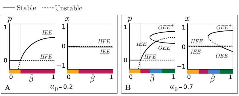
Figure 1: Bifurcation diagrams for (A) $u_{0}=0.2$ and (B) $u_{0}=0.7$. For $u_{0}=0.7$, in the region where $\bar{\beta}<\delta$ (yellow), the only stable fixed point in the interpretable range is the IIFE. A transcritical bifurcation occurs when $\bar{\beta}=\delta$. For $\delta<\bar{\beta}<\bar{\beta}^{*}$ (red), the IIFE is unstable and the IEE is stable. In these two regions, the system behaves exactly like the standard scalar SIS model. For $\bar{\beta}\in(\bar{\beta}^{*},\frac{\delta k_{p}}{k_{p}+u_{0}-1})$ (blue), two new fixed points given implicitly by the roots of (7) exist, the OEE⁺ and the OEE^-, the first is stable, and the latter unstable. In this region, the IIFE is unstable, and the IEE is stable. Finally, at $\bar{\beta}=\frac{\delta k_{p}}{k_{p}+u_{0}-1}$ the IEE exchanges stability with OEE^- in a transcritical bifurcation. For $\bar{\beta}>\frac{\delta k_{p}}{k_{p}+u_{0}-1}$ (green), the only stable equilibria are the OEE⁺ and the OEE^-. Parameters: $k_{x}=0.3,k_{p}=0.7,\delta=0.3$.

In Theorem IV.2 we proved that small urgency results in behavior equivalent to the SIS model. This result is illustrated in the bifurcation diagrams of Fig. 1A.

Next, we focus on the case where $f_{2}(x)$ has two real roots $x^{*}_{+}$ and $x^{*}_{-}$, where $x^{*}_{+}\geq x^{*}_{-}$. Let $\bar{\beta}^{*}$ be the value for which, given a set of parameters $\delta,k_{p},k_{x},u_{0}$, $f_{2}(x)$ has exactly one solution. We show that the NOD-SIS model has richer dynamics than the standard SIS model by proving the existence of a bifurcation of the IEE for $\bar{\beta}>\delta$. We will refer to any equilibrium of (2),(3) for which $x\neq 0$ and $p\neq 0$ as an Opinionated Endemic Equilibrium (OEE).

Theorem IV.3.

Let $x^{*}_{+}$ and $x^{*}_{-}$ be the two roots of the function in (7) with $x^{*}_{+}\geq x^{*}_{-}$ and let OEE${}^{+}=(p^{*}_{+},x^{*}_{+})$ and OEE${}^{-}=(p^{*}_{-},x^{*}{-})$, where $p^{*}_{\pm}=1-\frac{\delta}{\bar{\beta}(1+x^{*}_{\pm})}$. Let $\bar{\beta}>\delta$. Under Assumption 1, the system from (2) and (3) undergoes a transcritical bifurcation at $\bar{\beta}^{*}=\frac{\delta k_{p}}{k_{p}-1+u_{0}}$. In a small neighborhood of $(p,x,\bar{\beta})=\left(1-\frac{\delta}{\bar{\beta}^{*}},0,\bar{\beta}^{*}\right)$, OEE⁺ exists for $\bar{\beta}<\bar{\beta}^{*}$ and is unstable, and OEE⁺ exists for $\bar{\beta}>\bar{\beta}^{*}$ and is locally asymptotically stable.

Proof.

We perform a Lyapunov-Schmidt reduction. Following the steps outlined in [18, §3 p.33] we compute the leading coefficients of the normal form of the projection of (2),(3) onto the span of the right null eigenvector of

$$J\left(1-\frac{\delta}{\bar{\beta}},0\right)=\begin{bmatrix}\frac{\delta(u_{0}-1)}{k_{p}+u_{0}-1}&\frac{\delta(1-u_{0})}{k_{p}}\\ 0&0\end{bmatrix}$$ (8)

evaluated at $\beta=0$, where $\beta=\bar{\beta}-\frac{\delta k_{p}}{k_{p}+u_{0}-1}$, $g_{y}=g_{\beta}=g_{\beta\beta}=0$, $g_{yy}=2(k_{p}+u_{0}-1)\neq 0$, and $g_{\beta y}=\frac{(k_{p}+u_{0}-1)^{2}}{\delta k_{p}}>0$. Thus, from [18, Proposition 9.3], we establish the existence of a transcritical bifurcation and the stability of the solution branches. ∎

Fig. 1B illustrates the secondary bifurcation whose existence was established in Theorem IV.3. Observe that when $u_{0}<k_{p}(\delta-1)+1$, the second bifurcation point $\bar{\beta}^{*}\notin[0,1]$. Fig. 1 shows that the solution branch corresponding to OEE⁺ folds back on itself and regains stability. For all values $\bar{\beta}>\bar{\beta}^{*}$ there is in fact a bistability between OEE⁺ and OEE^-. The bifurcation diagram in Fig. 1 can be understood as a non-persistent unfolding of a pitchfork bifurcation [18, §Ic]. Note that the fixed points OEE⁺ and OEE^- correspond to risk seeking and risk aversion strategies, respectively. In the following corollary, we establish that risk seeking increases infection levels and risk aversion decreases infection levels from the baseline SIS predictions. We also prove that whether convergence is to OEE⁺ or to OEE^- is determined by the initial opinion. Let $p_{EE}^{*}=1-\frac{\delta}{\bar{\beta}}$ be the endemic infection levels of the standard SIS model (1).

Corollary IV.1 (Risk Seeking and Risk Aversion).

Consider (2),(3). Let Assumption 1 hold and let $u_{0}$ be such that $f_{2}(x)=0$ has exactly two real roots and such that $\frac{k_{p}\delta}{k_{p}+u_{0}-1}<1$. Take $\bar{\beta}>\frac{k_{p}\delta}{k_{p}+u_{0}-1}$. Define $\Omega_{S}=[0,1]\times[0,1]$ and $\Omega_{A}=[0,1]\times[-1,0]$. Then the following statements hold.

i) There are exactly four equilibria: the IIFE, IEE, OEE⁺, OEE^-;

ii) If $x(0)>0(<0)$, then $x(t)>0(<0)$ for all $t>0$. Furthermore, $\lim_{t\to\infty}(p(t),x(t))=(p^{*}_{+},x^{*}_{+})$ for all initial conditions in the interior of $\Omega_{S}$;

iii) $p^{*}_{-}\leq p_{EE}^{*}\leq p^{*}_{+}.$

Proof.

i) Since $f_{2}(x)=0$, this claim follows by analogous nullcline arguments as the proof of Theorem IV.2; ii) Observe that the set $[0,1]\times\{0\}$ is invariant under the flow of (2), (3). Recall from Theorem III.1 that $\Omega=[0,1]\times[-1,1]$ is forward invariant. Since $[0,1]\times\{0\}$ partitions $\Omega$ into $\Omega_{S}$ and $\Omega_{A}$ and no flow crosses the boundary, the two sets are themselves forward invariant. Next, observe that OEE${}^{+}\in\Omega_{S}$ and OEE${}^{-}\in\Omega_{A}$ are interior points; recall that the IIFE and IEE are unstable under the parameter assumptions of the Theorem following Theorems IV.1 and IV.3. Observe that the off-diagonal entries of the Jacobian matrix of (2),(3) are $J_{12}(p,x)=\bar{\beta}(1-p)p$ and $J_{21}(p,x)=\frac{k_{p}}{\tau_{x}}x\operatorname{sech}^{2}((k_{p}p+k_{x}x^{2}+u_{0})x)$. Observe that in $\Omega_{S}$, $J_{12}(p,x)\geq 0$ and $J_{21}(p,x)\geq 0$ which means the system is cooperative and therefore monotone in $\Omega_{S}$, and by [21, Theorem 3.22], the $\omega$-limit set for any trajectory starting in the interior of $\Omega_{S}$ is a single equilibrium. Since OEE⁺ is the only equilibrium in the set interior, we conclude that all trajectories inside $\Omega_{S}$ approach OEE⁺ as $t\to\infty$. iii) The steady-state infection values $p_{-}^{*}$ and $p_{+}^{*}$ satisfy $p^{*}_{\pm}=1-\frac{\delta}{\bar{\beta}(1+x^{*}_{\pm})}$; then $p^{*}_{\pm}-p^{*}_{EE}=\frac{\delta}{\bar{\beta}}\left(\frac{x^{*}_{\pm}}{1+x^{*}_{\pm}}\right)$ and $\operatorname{sign}(p^{*}_{\pm}-p^{*}_{EE})=\operatorname{sign}(x^{*}_{\pm})$ as long as $|x^{*}_{\pm}|<1$, where $x^{*}_{+}$ and $x^{*}_{-}$ are the positive and negative roots of $f_{2}$ in (7). ∎

In Fig. 1 we see bifurcation diagrams for the system when $u_{0}=0.2,0.7$. We see that the IIFE and IEE exchange stability when $\bar{\beta}=\delta$, and at $\bar{\beta}=\frac{\delta k_{p}}{k_{p}+u_{0}-1}$, the system undergoes a second bifurcation where the IEE and the OEE^- exchange stability. In this regime and for large $\bar{\beta}$, the system settles in a bistable endemic state where opinion and infection levels are determined completely by the sign of $x(0)$, and risk aversion results in lower infection than risk seeking. Fig. 2 shows trajectories for random initial conditions when $u_{0}=0.7$ and $\bar{\beta}$ varies in $[0,1]$. These trajectories show that small $\bar{\beta}<\frac{k_{p}\delta}{k_{p}+u_{0}-1}$ leads to behavior of the SIS model, while for $\bar{\beta}>\frac{k_{p}\delta}{k_{p}+u_{0}-1}$, the richer dynamics of the NOD-SIS model distinguish the risk seeking and aversion strategies.

Figure 2: Trajectories for $12$ random initial conditions for $\bar{\beta}=0.25$, $\bar{\beta}=0.36$, $\bar{\beta}=0.44$, and $\bar{\beta}=0.75$, that correspond to each of the regions (yellow, red, blue and green) of Fig. 1B when $u_{0}=0.7$. The black line in the infection plots is the endemic equilibrium of the standard SIS model. In the yellow and red regions, the system converges to the IIFE and IEE, respectively. In the blue region, agents who begin with an averter strategy converge to the endemic equilibrium of the SIS model, while agents who start with a risk seeking strategy converge to a higher infection level. In the green region, the system’s trajectories converge to one of the two opinionated equilibria determined by the initial opinions. Parameters: $\delta=0.3,k_{p}=0.7,k_{x}=0.3,\tau_{x}=1$.

In the following section, we explore numerically the case when the opinion feedback gain $k_{x}$ is high, and the function defined in (6) is not convex. We see that for certain parameter regimes, risk aversion allows the complete eradication of infection, while risk seeking increases infection levels.

IV-B Strong Peer Pressure

In this section we explore numerically the behavior of the system when peer pressure is large. We see that a stable Opinionated Infection Free Equilibrium (OIFE) exists with the risk averter strategy, and a symmetric stable OIFE point does not exist with the risk seeking or risk-neutral strategy. We begin by stating the following remark:

Remark IV.1.

For $k_{x}>\frac{1}{3}$, the function defined in (6) is not convex, and we can find $u_{0}$, $k_{p}$ and $k_{x}$ such that $f_{1}(x)=0$. The solutions to this equation correspond to null infection and non-zero opinion levels, and do not depend on the values of $\delta$ and $\bar{\beta}$. Thus, even for a large value of $\bar{\beta}$, associated with very infectious diseases, an OIFE exists.

In numerical simulations we see that only one of the OIFE associated to the roots of $f_{1}(x)$ is stable, and it corresponds to negative opinion levels. We see that the steady-state behavior is determined by $\text{sign}(x(0))$. When $x(0)<0$, i.e., when the initial opinion is towards risk aversion, then the population is able to reach the stable OIFE and thus eliminate the disease. If $x(0)>0$, the population reaches an OEE, and the infection levels are higher than the EE in the SIS. This demonstrates an absence of symmetry in infection levels associated with the different strategies. It suggests that in a population with high sensitivity to opinion levels and urgency levels, choosing an aversion strategy is beneficial as it leads to an infection-free state. We leave the analysis of the equilibria and bifurcations of the model in this parameter regime for future work.

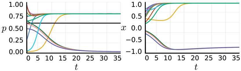
Figure 3: Initial opinion towards the risk seeking or aversion strategy is reinforced in a population with high peer pressure, and the sign of initial opinions are determinant of the infection levels at steady state. Initial averters reach an infection-free state, while initial risk seekers reach an endemic state with higher infection levels than the endemic equilibrium of the standard SIS infection level, represented by a thick black line. Parameters: $\delta=0.3,\bar{\beta}=0.75,u_{0}=0.9,k_{p}=0.7,k_{x}=0.7.$

V Numerical Simulations for Structured Populations

We explore the behavior of the NOD-SIS model in structured populations. We consider two networks with corresponding graph adjacency matrices $A$ and $\hat{A}$. $A$ represents the physical contacts between subpopulations: edge $(i,j)\in E(A)$ if and only if subpopulation $i$ has physical contact with subpopulation $j$. $\hat{A}$ encodes communication in, for example, a social online network: edge $(i,j)\in E(\hat{A})$ if and only if subpopulation $i$ shares information about infection levels with subpopulation $j$. We assume $A$ and $\hat{A}$ are symmetric. The NOD-SIS model dynamics are

$$\dot{p}_{j} =\bar{\beta}(1+x_{j})(1-p_{j})\sum_{k=1}^{N}a_{jk}p_{k}-\delta_{j}p_{j},$$ (9)

$$\tau_{x}\dot{x}_{j} =-x_{j}+\tanh\left(u_{j}\cdot\left(\alpha_{j}x_{j}+\sum_{\begin{subarray}{c}k=1\\ k\neq j\end{subarray}}^{N}\hat{a}_{jk}x_{k}\right)\right),$$ (10)

$$u_{j} =k_{p}\frac{1}{\hat{d}_{j}}\sum_{k=1}^{N}\left|\hat{a}_{jk}\right|p_{k}+k_{x}\sum_{k=1}^{N}\hat{a}_{jk}x_{j}^{2}+u_{0}.$$ (11)

We assume $\delta_{j}=\delta$, and that $\alpha_{j}=0$ for all $j\in\{1,\ldots,N\}$, that is, all individuals recover at the same rate $\delta$. The interpretation for $\alpha_{j}=0$ is no opinion self-reinforcement.

We first compare this system with the standard network SIS model [20]. In Fig. 4, we see two examples of $A$ and $\hat{A}$. $A$ is a wheel graph with $5$ nodes, and $\hat{A}$ is a complete graph of the same size. We first explore the case where all the edges of $\hat{A}$ are positive, as it describes a cooperation between subpopulations. For these two networks, we explore how the trajectories behave in comparison to the standard network SIS model for different sets of initial conditions. We observe that cooperation makes all subpopulations reach either a risk seeking or risk aversion strategy, and this common choice determines the infection levels at steady state. As in the well-mixed case, common risk aversion results in lower infection levels for all subpopulations as compared to the standard networks SIS case, while risk seeking behavior increases infection levels. In Fig. 5 we explore how antagonism affects trajectories in the network setting. We see that if $\hat{A}$ has negative-weight edges, then different populations will settle at different strategies. Risk-aversion populations reach lower infection levels than risk seeking populations. Future work will explore how the topology of the contact and communication networks determines infection levels.

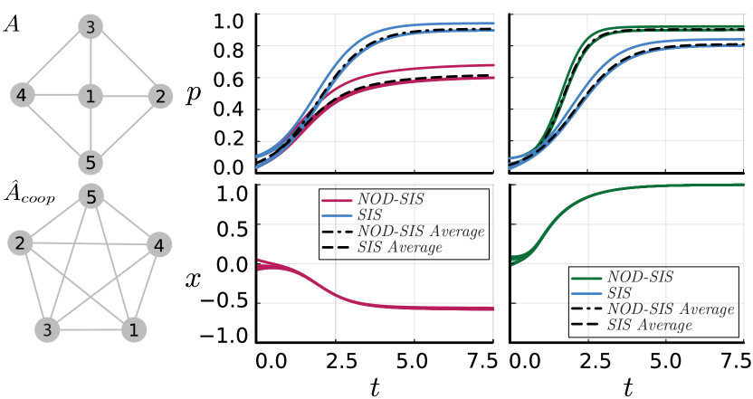
Figure 4: Contact and communication graphs $A$ and $\hat{A}_{coop}$ (left) for $5$ subpopulations where cooperation between populations is present. We see that populations reach a state of agreement for either risk aversion (middle) or risk seeking (right). The strategy chosen determines infection levels, and aversion reduces infection levels with respect to the standard network SIS model for the same initial conditions, while risk seeking increases infection levels. Parameters: $\bar{\beta}=0.5,\delta=0.3,k_{p}=0.5,k_{x}=0.3,u_{0}=0.7$.

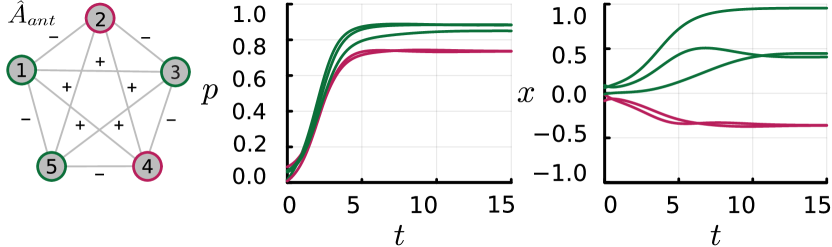
Figure 5: Antagonism between populations as in the communication network $\hat{A}_{ant}$ (left) and $A$ as in Fig. 4 results in disagreement and some populations choose risk aversion (red) and others choose a risk seeking strategy (green). As in the well-mixed setting, risk aversion reduces infection while risk seeking increases infection levels. Parameters: $\bar{\beta}=0.5,\delta=0.3,k_{p}=0.5,k_{x}=0.3,u_{0}=0.7$.

VI Conclusion and Future Directions

We have presented the NOD-SIS model to couple the epidemiological SIS model with opinion dynamics in a well-mixed population. For low peer pressure and low infectiousness, the system behaves locally like the standard SIS model. For higher infectiousness, the system presents a state of bistability where a population’s initial opinion for risk seeking or risk aversion increases or decreases the steady-state infection levels when compared to the basal SIS model. For high peer pressure and high basal urgency, the system presents an infection-free opinionated equilibrium that can be reached with initial risk aversion.

We explored the NOD-SIS model in a structured population using two networks among subpopulations: a contact network to model infection spread and a communication network to model information spread. When the communication network is cooperative, all subpopulations choose risk aversion or all choose risk seeking. As in the well-mixed setting, risk aversion (seeking) decreases (increases) infection levels relative to the infection levels of the network SIS. When the communication network has antagonistic interactions, the system reaches a state of disagreement where some populations choose risk aversion and some choose risk seeking. Averters reach lower infection levels than risk seekers. In future work we will analyze the dynamical properties in the network setting and explore how topologies of the two different network influence the system’s outcomes.

References

- [1] L. Yang, S. M. Constantino, B. T. Grenfell, E. U. Weber, S. A. Levin, and V. V. Vasconcelos, “Sociocultural determinants of global mask-wearing behavior,” Proceedings of the National Academy of Sciences, vol. 119, no. 41, p. e2213525119, 2022.
- [2] Z. Qiu, B. Espinoza, V. V. Vasconcelos, C. Chen, S. M. Constantino, S. A. Crabtree, L. Yang, A. Vullikanti, J. Chen, J. Weibull, et al., “Understanding the coevolution of mask wearing and epidemics: A network perspective,” Proceedings of the National Academy of Sciences, vol. 119, no. 26, p. e2123355119, 2022.
- [3] O. N. Bjørnstad, K. Shea, M. Krzywinski, and N. Altman, “Modeling infectious epidemics.,” Nature methods, vol. 17, no. 5, pp. 455–457, 2020.
- [4] Y. Zhou, S. A. Levin, and N. E. Leonard, “Active control and sustained oscillations in actsis epidemic dynamics,” IFAC-PapersOnLine, vol. 53, no. 5, pp. 807–812, 2020.
- [5] A. Bizyaeva, M. O. Arango, Y. Zhou, S. Levin, and N. E. Leonard, “Active risk aversion in sis epidemics on networks,” in 2024 American Control Conference (ACC), pp. 4428–4433, IEEE, 2024.
- [6] Q. Wu and S. Chen, “Coupled simultaneous evolution of disease and information on multiplex networks,” Chaos, Solitons & Fractals, vol. 159, p. 112119, 2022.
- [7] K. Peng, Z. Lu, V. Lin, M. R. Lindstrom, C. Parkinson, C. Wang, A. L. Bertozzi, and M. A. Porter, “A multilayer network model of the coevolution of the spread of a disease and competing opinions,” Mathematical Models and Methods in Applied Sciences, vol. 31, no. 12, pp. 2455–2494, 2021.
- [8] B. She, J. Liu, S. Sundaram, and P. E. Paré, “On a networked sis epidemic model with cooperative and antagonistic opinion dynamics,” IEEE Transactions on Control of Network Systems, vol. 9, no. 3, pp. 1154–1165, 2022.
- [9] W. Xuan, R. Ren, P. E. Paré, M. Ye, S. Ruf, and J. Liu, “On a network sis model with opinion dynamics,” IFAC-PapersOnLine, vol. 53, no. 2, pp. 2582–2587, 2020.
- [10] Y. Lin, W. Xuan, R. Ren, and J. Liu, “On a discrete-time network sis model with opinion dynamics,” in 2021 60th IEEE Conference on Decision and Control (CDC), pp. 2098–2103, IEEE, 2021.
- [11] M. Ye, L. Zino, A. Rizzo, and M. Cao, “Game-theoretic modeling of collective decision making during epidemics,” Physical Review E, vol. 104, no. 2, p. 024314, 2021.
- [12] K. Frieswijk, L. Zino, M. Ye, A. Rizzo, and M. Cao, “A mean-field analysis of a network behavioral–epidemic model,” IEEE Control Systems Letters, vol. 6, pp. 2533–2538, 2022.
- [13] F. B. Agusto, I. V. Erovenko, A. Fulk, Q. Abu-Saymeh, D. Romero-Alvarez, J. Ponce, S. Sindi, O. Ortega, J. M. Saint Onge, and A. T. Peterson, “To isolate or not to isolate: the impact of changing behavior on covid-19 transmission,” BMC Public Health, vol. 22, no. 1, p. 138, 2022.
- [14] S. Funk, M. Salathé, and V. A. Jansen, “Modelling the influence of human behaviour on the spread of infectious diseases: a review,” Journal of the Royal Society Interface, vol. 7, no. 50, pp. 1247–1256, 2010.
- [15] J. Bedson, L. A. Skrip, D. Pedi, S. Abramowitz, S. Carter, M. F. Jalloh, S. Funk, N. Gobat, T. Giles-Vernick, G. Chowell, et al., “A review and agenda for integrated disease models including social and behavioural factors,” Nature human behaviour, vol. 5, no. 7, pp. 834–846, 2021.
- [16] A. Bizyaeva, A. Franci, and N. E. Leonard, “Nonlinear opinion dynamics with tunable sensitivity,” IEEE Transactions on Automatic Control, vol. 68, no. 3, pp. 1415–1430, 2023.
- [17] N. E. Leonard, A. Bizyaeva, and A. Franci, “Fast and flexible multiagent decision-making,” Annual Review of Control, Robotics, and Autonomous Systems, vol. 7, 2024.
- [18] M. Golubitsky and D. G. Schaeffer, Singularities and Groups in Bifurcation Theory, vol. 51 of Applied Mathematical Sciences. New York, NY: Springer-Verlag, 1985.
- [19] F. Blanchini, S. Miani, et al., Set-theoretic methods in control, vol. 78. Springer, 2008.
- [20] W. Mei, S. Mohagheghi, S. Zampieri, and F. Bullo, “On the dynamics of deterministic epidemic propagation over networks,” Annual Reviews in Control, vol. 44, pp. 116–128, 2017.
- [21] M. W. Hirsch and H. Smith, “Monotone dynamical systems,” Handbook of differential equations: ordinary differential equations, vol. 2, pp. 239–357, 2006.