Forcing Planets to Evolve: The Relationship Between Uranus and Neptune at Late Stages of Dynamical Evolution

Abstract

The dynamical properties of the bodies in the outer Solar System hold information regarding the planets’ orbital histories. In early Solar System numerical simulations, where chaos is a primary driver, it is difficult to explore parameter space in a systematic way. In such simulations, stable configurations are hard to come by, and often require special fine-tuning. In addition, it is infeasible to run suites of well-resolved, realistic simulations with massive particles to drive planetary evolution where enough particles remain to represent the transneptunian populations to robustly statistically compare with observations. To complement state of the art full N-body simulations, we develop a method to artificially control each planet’s orbital elements independently from each other, which when carefully applied, can be used to test a wider suite of models. We modify two widely used publicly available N-body integrators: (1) the C code, REBOUND and (2) the FORTRAN code, Mercury. We show how the application of specific fictitious forces within numerical integrators can be used to tightly control planetary evolution to more easily explore migration and orbital excitation and damping. This tool allows us to replicate the impact a massive planetesimal disk would have on the planets, without actually including the massive planetesimals, thus decreasing the chaos and simulation runtime. We highlight an appropriate application that shows the impact of Neptune’s eccentricity damping and radial outward migration on Uranus’ eccentricity.

1 Introduction

Planets’ orbits evolve through long and short term interactions with gas, planetesimals, and nearby planets (e.g., Chambers, 2009; Dawson & Johnson, 2018; Armitage, 2011; Andrews, 2020; Wyatt, 2008; Hughes et al., 2018; Pearce, 2024; Morbidelli & Levison, 2014; Levison & Dones, 2014; Morbidelli & Nesvorný, 2020; Horner et al., 2020; Fernandez & Ip, 1984; Goldreich et al., 2004). When modeling planetary evolution caused by gravitational interactions with millions of small bodies, simplifications are necessary to address an otherwise computationally infeasible problem. A common approach in simplifying and decreasing the computational cost of an N-body simulation is to artificially evolve a planet’s semimajor axis, eccentricity, and/or inclination. This is particularly important for science cases in which it is necessary to track the evolution of a statistically significant sample of planetesimals distinct from those driving the planetary evolution. For example, when studying the evolution of the outer solar system, artificially controlling the giant planets evolution is helpful so that the particles representing the Trans Neptunian Objects (TNOs) can be massless, increasing the number that can be modeled and tracked, and their final dynamical configuration can be compared to currently observed distributions and used to constrain evolution models.

Artificial evolution has been widely done with "user-defined forces" where the code user defines an expression for the acceleration that will be added on top of the direct gravitational acceleration of the object due to other bodies in the simulation at each timestep (e.g., Malhotra, 1995; Hahn & Malhotra, 2005; Wolff et al., 2012; Lee & Peale, 2002; Ali-Dib et al., 2021). In celestial mechanics, force and acceleration are used interchangeably due to their proportional relationship for a given mass; for clarity, we will only refer to these as accelerations. In this paper we show how applying a "user-defined velocity" as well as a user-defined acceleration provides a complementary approach to what has been done before by granting stronger control over the bodies’ evolution, allowing each orbital element to be evolved independently from each other. Including user-defined velocities and accelerations in an N-body simulation mimics the presence of a physical process by updating the position and velocity of the particle at every time step. For example, one can emulate planets exchanging angular momentum with a disk of planetesimals by knowing how the orbital elements are expected to evolve with time for such a process. We extend the philosophy of user defined accelerations further by introducing user defined velocities into two widely used N-body integrators: (1) the publicly available C code, REBOUND (Rein & Liu, 2012; Rein & Tamayo, 2015; Rein et al., 2019) and (2) the FORTRAN code, Mercury6.2 (Chambers, 1999).

The use of artificial velocities and accelerations within numerical integrators is powerful when tight control of planets’ orbital evolution is desired. An example application is a chaotic evolution where minuscule changes to the initial parameters can produce a vastly different final configuration. Such chaos hinders the exploration of a large parameter space because the final outcomes are unpredictable. For example, in the well-studied planetary instability model of the outer solar system, a chaotic, planet-planet scattering phase is followed by a damping phase where the planetesimal disk is responsible for damping Neptune’s and Uranus’ eccentricities and migrating the planets outward. For this type of simulation, hundreds of runs are necessary just to get one that qualitatively matches the current planet configuration, making this a computationally expensive problem (e.g. Tsiganis et al., 2005; Levison et al., 2008; Clement et al., 2018; de Sousa et al., 2020). Individual control of the planets’ orbital elements is useful here in allowing exploration of a larger parameter space after the chaotic phase. While it is unphysical for the orbital elements to evolve independently (eccentricity and semimajor axis are coupled, for example), the use of this tool is appropriate when the orbits’ time evolution due to a physical process is known through analytical derivations and/or existing full N-body simulations. In this case, the time evolution of the eccentricity and semimajor axis of the planets due to angular momentum and energy exchange with the planetesimals is well-characterized by a function. Gravitational interactions between planetesimals and planets—Neptune in particular—sculpt the outer regions of the planetesimal disk over million and billion-year timescales. To rigorously compare simulations with observations, the final outcome of the planets must match their current observed orbits, where the possibility of such an evolution can be assessed by comparing the particle disk configuration to the dynamical structure of TNOs. Even in simulations where planet-planet scattering is not a major driver, planets often still need an extra push to arrive at the necessary location for detailed comparisons with observations.

To demonstrate an appropriate use of artificial orbital evolution, we focus on one class of frequently studied planet instability model: the simulation shown in Figure 1 of Tsiganis et al. (2005) (see Section 4). The planet-planet scattering phase produces unpredictable intermediate outcomes because of their chaotic nature, whereas Uranus’ and Neptune’s eccentricity damping phases are caused by dynamical friction. In addition, individual control of planet’s evolution is useful when one is interested in isolating the impact of gravitational interactions between specific bodies while avoiding other interactions that are also at play. An interesting outcome of evolving planets individually is noticing that eccentricity damping of one planet can cause another planet’s eccentricity to decline due to their secular coupling, as seen in Levison et al. (2011); Greenberg et al. (2013); Hansen & Murray (2015).

The procedure described in this paper is most useful when

1. the final state of a well-understood evolution process must be tuned to reach the current state of an observed system for detailed comparison with observations

2. a parameter space exploration of chaotic evolution that ends at a desired outcome is infeasible in full n-body simulations due to computational expense, unpredictability, and the size of the parameter space

3. a planet’s orbital evolution due to physical processes the user wants to mimic in the simulation is well-described by time-dependant functions for the orbital parameters

In Section 2, we introduce the analytical framework for adding fictitious forces and velocities to the equations of motion and then describe modifications to the n-body codes Mercury 6.2 and REBOUND. In Section 3, we show examples with one and two planets where each planet’s orbital elements are evolved with arbitrary functions. In Section 4 we demonstrate two appropriate applications for when this code is useful. We show how we successfully reproduce the outward migration and eccentricity damping exhibited by Uranus and Neptune in a well-known Nice model simulation (Tsiganis et al., 2005). We also show that it is important to consider the secular coupling between Neptune and Uranus in the late-stages of orbital damping by planetesimals. As Neptune’s eccentricity damps, Uranus’ eccentricity damps indirectly as well. In Section 5 we summarise our results and discuss further applications for this code.

2 Modification to The Equations of Motion

We aim to adjust a simulated planet’s orbit such that, if no other perturbers were present in the simulation, each orbital element would independently evolve according to a specified function. The prescribed functions encapsulate the effects of processes not included in the simulation. Note that in simulations with multiple planets, since the planet is also accelerated by other system planets, the prescribed functions do not determine the full evolution of the orbit.

Additional forces are an existing functionality of REBOUND and Mercury6.2, where an arbitrary force can be added to a particle of choice every time-step, which operationally updates the particle’s velocity every time-step. However, it is not possible to fully and independently evolve a planet’s orbital elements using only additional forces. For full control, we require an update to the position of the planet at each time step (to account for changes to the velocity) as well as an update to the velocity. To calculate the required updates, we take partial derivatives of the equations of motion with respect to each orbital element to then form a fictitious velocity and acceleration to evolve the object given a functional form. This keeps the evolution of each orbital element independent from the others.

Physical accelerations such as radiation forces, gas dynamical friction, and more, are already incorporated onto REBOUND through the library REBOUNDx. The library contains eccentricity and inclination damping, but the only free parameter the user can choose is a damping timescale. With our modifications to REBOUND, rather than coding in individual physical effects, we can code arbitrary functional forms for how the elements should evolve. While this is nonphysical, these modifications allow us to probe a large amount of parameter space and various dynamical histories to learn how they impact the structure and dynamics of systems.

We follow Lee & Peale (2002) and expand on the work of Dawson & Murray-Clay (2012) and Wolff et al. (2012) to derive modifications to the equations of motion of an orbiting body to allow any form of evolution of the body’s orbital elements. Modifications to REBOUND and Mercury6.2 are outlined in Appendix A.

2.1 Analytical Derivation of Forces and Velocities for Arbitrary Orbital Element Evolution

The position and velocity of an orbiting body in Cartesian coordinates, ($x,y,z,\dot{x},\dot{y},\dot{z}),$ can be fully described by the six osculating orbital elements: semimajor axis ($a$), eccentricity ($e$), inclination ($i$), argument of pericenter ($\omega$), longitude of ascending node ($\Omega$), and true anomaly ($f$). In other words, $x=x(a,e,i,\omega,\Omega,f)$ and so on for the other five Cartesian coordinates. The total time derivative of the $x$-component of the body’s velocity and acceleration can thus be written as

$$\large\frac{dx}{dt}=\frac{\partial x}{\partial a}\dot{a}+\frac{\partial x}{\partial e}\dot{e}+\frac{\partial x}{\partial i}\dot{I}+\frac{\partial x}{\partial\omega}\dot{\omega}+\frac{\partial x}{\partial\Omega}\dot{\Omega}+\frac{\partial x}{\partial f}\dot{f}$$ (1a)

$$\large\frac{d\dot{x}}{dt}=\frac{\partial\dot{x}}{\partial a}\dot{a}+\frac{\partial\dot{x}}{\partial e}\dot{e}+\frac{\partial\dot{x}}{\partial i}\dot{I}+\frac{\partial\dot{x}}{\partial\omega}\dot{\omega}+\frac{\partial\dot{x}}{\partial\Omega}\dot{\Omega}+\frac{\partial\dot{x}}{\partial f}\dot{f}$$ (1b)

and similarly for $y$, $\dot{y}$, $z$ and $\dot{z}$. Note that we have used $\dot{I}$ to indicate $di/dt$ for notational clarity.

In the two body problem, $a$, $e$, $i$, $\omega$, and $\Omega$ remain constant in time, and $\dot{f}$ provides the only non-zero orbital element time derivative in each of the expressions in Equation (1). In other words, the central body in a two-body simulation generates evolution of the form $dx/dt=(\partial x/\partial f)\dot{f}$ and so on for the other Cartesian elements. This evolution occurs, by construction, on the timescale of an orbital period. The term $\dot{f}$ is related to the angular momentum by the equation $r^{2}\dot{f}=h=na^{2}\sqrt{1-e^{2}}$, so that

$$r\dot{f}=na\frac{1+e\cos{f}}{\sqrt{1-e^{2}}}$$ (2)

where $r=\frac{a(1-e^{2})}{1+e\cos{f}}$ is the radial distance from the central body, $n=\sqrt{\frac{GM}{a^{3}}}$ is the mean motion, $G$ is the gravitational constant, and $M$ is the total mass of the system.

We are interested in inducing orbital element evolution on timescales much longer than the orbital period, so we separate Equations (1) into the first five terms, which we will evolve by hand using arbitrary functions for $\dot{a}$, $\dot{e}$, $\dot{i}$, $\dot{\omega}$, and $\dot{\Omega}$, and, separately, the $\dot{f}$ term. For N-body problems, the force of the central body changes $f$ by the form of Equation (2), so we do not need to prescribe an artificial evolution for this element.

Recall that the osculating orbital elements $a$, $e$, $i$, $\omega$, $\Omega$, and $f$ by definition are related to the Cartesian positions $x$, $y$, $z$ by

$$x =r\cos{\Omega}\cos{(\omega+f)}-r\cos{i}\sin{\Omega}\sin{(\omega+f)}$$ (3a)

$$y =r\sin{\Omega}\cos{(\omega+f)}+r\cos{i}\cos{\Omega}\sin{(\omega+f)}$$ (3b)

$$z =r\sin{i}\sin{(\omega+f)}$$ (3c)

where $r$ is not an orbital element, but a function of three orbital elements, $r=r(a,e,f)$. The Cartesian velocity components of the orbiting body are then the time derivative of Equation (3), allowing all elements to vary with time:

$$\dot{x} =\dot{r}\cos{\Omega}\cos{(\omega+f)}-r\sin{\Omega}\dot{\Omega}\cos{(\omega+f)}$$ (4a)

$$-(r\dot{\omega}+r\dot{f})\cos{\Omega}\sin{(\omega+f)}-\dot{r}\cos{i}\sin{\Omega}\sin{(\omega+f)}$$

$$+r\sin{i}\dot{I}\sin{\Omega}\sin{(\omega+f)}-r\cos{i}\cos{\Omega}\dot{\Omega}\sin{(\omega+f)}$$

$$-(r\dot{\omega}+r\dot{f})\cos{i}\sin{\Omega}\cos{(\omega+f)}$$

$$\dot{y} =\dot{r}\sin{\Omega}\cos{(\omega+f)}+r\cos{\Omega}\dot{\Omega}\cos{(\omega+f)}$$ (4b)

$$-(r\dot{\omega}+r\dot{f})\sin{\Omega}\sin{(\omega+f)}+\dot{r}\cos{i}\cos{\Omega}\sin{(\omega+f)}$$

$$-r\sin{i}\dot{I}\cos{\Omega}\sin{(\omega+f)}-r\cos{i}\sin{\Omega}\dot{\Omega}\sin{(\omega+f)}$$

$$+(r\dot{\omega}+r\dot{f})\cos{i}\cos{\Omega}\cos{(\omega+f)}$$

$$\dot{z} =\dot{r}\sin{i}\sin{(\omega+f)}+r\cos{i}\dot{I}\sin{(\omega+f)}$$ (4c)

$$+(r\dot{\omega}+r\dot{f})\sin{i}\cos{(\omega+f)}$$

where we define $\dot{r}=\frac{\partial r}{\partial a}\dot{a}+\frac{\partial r}{\partial e}\dot{e}+\frac{\partial r}{\partial f}\dot{f}$. Recall that in the two body problem, $\dot{r}$ is derived assuming $a$ and $e$ are constant in time, producing $\dot{r}=\frac{\partial r}{\partial f}\dot{f}=\frac{nae\sin{f}}{\sqrt{1-e^{2}}}$ (see Murray & Dermott 1999).

To independently control the evolution of a particle’s orbital elements, the particle’s position and velocity must be updated every timestep with a small additional perturbation to the momentum and force, or in other words, velocity and acceleration. Similar to Equation (1), we define a user-defined velocity and user-defined acceleration, which are given by

$$\large\dot{x}_{\rm user}=\frac{dx}{dt}=\frac{\partial x}{\partial a}\dot{a}+\frac{\partial x}{\partial e}\dot{e}+\frac{\partial x}{\partial i}\dot{i}+\frac{\partial x}{\partial\omega}\dot{\omega}+\frac{\partial x}{\partial\Omega}\dot{\Omega}$$ (5a)

$$\large\ddot{x}_{\rm user}=\frac{d\dot{x}}{dt}=\frac{\partial\dot{x}}{\partial a}\dot{a}+\frac{\partial\dot{x}}{\partial e}\dot{e}+\frac{\partial\dot{x}}{\partial i}\dot{i}+\frac{\partial\dot{x}}{\partial\omega}\dot{\omega}+\frac{\partial\dot{x}}{\partial\Omega}\dot{\Omega}$$ (5b)

and similarly for $\dot{y}_{\rm user}$, $\ddot{y}_{\rm user}$, $\dot{z}_{\rm user}$, and $\ddot{z}_{\rm user}$ where $\dot{a}$, $\dot{e}$, $\dot{i}$, $\dot{\omega}$, and $\dot{\Omega}$ are the arbitrary functions we define (see Section 3). The user-defined velocity and user-defined acceleration are added to the existing motion of the particles. For each time step, $\Delta t$, the $x$-position and $x$-velocity of the object are updated by a term $\dot{x}_{\rm user}\Delta t$ and $\ddot{x}_{\rm user}\Delta t$, respectively and similarly for $y$ and $z$. All of the partial derivatives used in Equation (5) and further discussion of our implementation in REBOUND and Mercury6.2 can be found in Appendix A.

3 One and two planet examples

We demonstrate the potential of our modifications to REBOUND and Mercury6.2 with two example simulations, one with a star and one planet and the other with a star and two planets. For both examples, we ran 50 million year REBOUND (MERCURIUS integrator) and Mercury6.2 (HYBRID integrator) simulations. To compare short term and long term planetary behavior between the two N-body codes, we ran simulations with the same initial conditions, type of integrator, and output cadence. The five orbital elements, $a$, $e$, $i$, $\omega$, $\Omega$ are evolved using user-defined velocities and accelerations (Equation 5) by defining a functional form for $\dot{a}$, $\dot{e}$, $\dot{i}$, $\dot{\omega}$, and $\dot{\Omega}$. For the examples in this section, we choose a combination of arbitrary functional forms for the orbital elements shown in Equation (6), where $g$ is a stand-in variable for any of the evolved orbital elements:

$$\dot{g}(t)=\frac{\Delta g}{(t+\tau_{g})}$$ (6a)

$$\dot{g}(t)=\frac{2\pi\Delta g}{\tau_{g}}\cos{\Big{(}2\pi\frac{t}{\tau_{g}}\Big{)}}$$ (6b)

$$\dot{g}(t)=\frac{\Delta g}{\tau_{g}}\exp{\Big{(}-\frac{t}{\tau_{g}}\Big{)}}$$ (6c)

$$\dot{g}(t)=\frac{\Delta g}{\tau_{g}}$$ (6d)

where $\Delta g$ is the scale of the change, $\tau_{g}$ is the timescale of the change, and $t$ is the time variable. Equation (6) corresponds to a time derivative of

$$g(t)=g_{0}+\Delta g\log{\Big{(}\frac{t}{\tau_{g}}+1\Big{)}}$$ (7a)

$$g(t)=g_{0}-\Delta g\sin{\Big{(}2\pi\frac{t}{\tau_{g}}\Big{)}}$$ (7b)

$$g(t)=g_{0}+\Delta g-\Delta g\exp{\Big{(}-\frac{t}{\tau_{g}}\Big{)}}$$ (7c)

$$g(t)=g_{0}+\Delta g\frac{t}{\tau_{g}}$$ (7d)

where $g_{0}$ is the initial value of the parameter. In future references to Equations (6) and (7), the variable $g$ is replaced by the orbital element we evolve.

In the code, a user has the freedom to write any desired function to evolve an orbital parameter, which can include a nonphysical time-evolution. We expect the user to define functions that are physically motivated by full N-body simulations or analytical models. We discuss this further in Section 4. The user-defined accelerations and velocities must remain small compared to the accelerations and velocities due to the other bodies in the simulation for the integrators to produce reasonable levels of accuracy. This is a constraint due to the symplectic Wisdom and Holman integrator mappings, while implementing a non-symplectic analytical equation of motion (Wisdom & Holman, 1991; Tamayo et al., 2020). If the additional force becomes comparable to the central gravitational force, we find that the one-planet simulations encounter large errors and eventually return nan values. We use the MERCURIUS and HYBRID integrators for REBOUND and Mercury6.2 respectively, because they use the Wisdom-Holman scheme and switch to an adaptive, high-accuracy integrator when particles undergo close encounters. During a close encounter between two bodies, the gravitational force increases significantly and changes the orbit quickly, therefore small time-steps are essential to accurately resolve the physics. The switch to an adaptive integrator is only triggered for close encounters however, so an additional large force and velocity, as we discuss in this paper, will not trigger the switch to an adaptive time-step, and will instead produce an inaccurate evolution.

For the single-planet example, we integrate the orbits of a solar-mass star and Jupiter-mass planet. To confirm that each element is evolved independently from the others, we ran several initial tests (not shown) evolving one element at a time as well as combinations of elements. We find that the signature of one orbital element’s evolution is apparent on other elements to a negligible degree. For example, when exponentially or sinusoidally evolving only the eccentricity ($e$) of the planet, the semi-major axis ($a$) evolution contains a residual signature of the same functional form, though it is only noticeable at a precision of one part in $10^{7}$ for REBOUND and one part in $10^{4}$ for Mercury6.2. The perturbation on the semi-major axis is more pronounced when $\dot{e}$ in Equation (5) is large, confirming that the user-defined velocities and accelerations must remain small compared to the central gravitational acceleration.

Figure 1 shows an example where we artificially evolve all orbital elements with arbitrary functions for $\dot{a}$, $\dot{e}$, $\dot{i}$, $\dot{\omega}$, and $\dot{\Omega}$. The Jupiter-mass planet is initialized at $a_{0}=5.2$ au, $e=0.2$, $i=10^{\circ}$, $\omega=50^{\circ}$, $\Omega=30^{\circ}$, and $f=240^{\circ}$. The parameters describing the artificial evolution of the planet are found in Table 1. Through the modifications described in Section 2 and Appendix A, we were able to successfully evolve all elements arbitrarily and independently from each other.

	$g_{0}$	$\Delta g$	$\tau_{g}$ (Myr)	Equation 7
$a$	5.2 au	1.8 au	10	logarithmic (a)
$e$	0.2	0.1	5	sinusoidal
$i$	10 deg	5 deg	4	exponential (c)
$\omega$	50 deg	35 deg	80	linear (d)
$\Omega$	30 deg	60 deg	20	sinusoidal (b)
$f$	240 deg	–	–	–

Table 1: Function and parameters for the one-planet example. Each orbital element’s time evolution is shown in Figure 1.

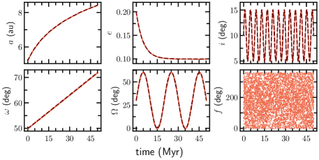
Figure 1: Fifty million year evolution of the semimajor axis ($a$ (au); top left), eccentricity ($e$; top middle), inclination ($i$ (deg); top right), argument of pericenter ($\omega$ (deg); bottom left), longitude of ascending node ($\Omega$ (deg); bottom middle), and true anomaly ($f$ (deg); bottom right) of a Jupiter-mass planet orbiting a solar-mass star. The planet is initialized with the orbital elements in column $g_{0}$ in Table 1. The orbital elements $a$, $e$, $i$, $\omega$, and $\Omega$ are artificially time evolved by the arbitrary functions (dashed line) in Equation (7), denoted by the last column in Table 1. Each orbital element in fact evolves independently from each other and follows the functional form prescribed in the code.

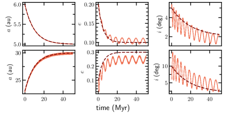
Figure 2: Fifty million year evolution of the semimajor axis ($a$), eccentricity ($e$), inclination ($i$) (orange) of a Jupiter-mass (top row) and Neptune-mass (bottom row) planet orbiting a solar-mass star. The orbital elements are initialized and artificially evolved by an exponential (dark maroon dashed line) with parameters described in Table 2. Similar to the one planet example in Figure 1, the additional user velocity and acceleration prescription evolves the orbital elements analogous to a desired function. However, the evolution of the eccentricity and inclination of each planet have a short timescale oscillation on top due to the secular effects between the planets. In contrast to the one planet example, where we can evolve the element to a final value, in this case the equation typically sets the minimum or maximum of the oscillation.

		$g_{0}$	$\Delta g$	$\tau_{g}$ (Myr)	Equation 7
	$a$	6 au	$-1$ au	10	exponential (c)
	$e$	0.2	$-0.1$	5	exponential (c)
planet 1	$i$	5 deg	$-3$ deg	20	exponential (c)
Jupiter-mass	$\omega$	50 deg	–	–	–
	$\Omega$	30 deg	–	–	–
	$f$	240 deg	–	–	–
	$a$	23 au	7.0 au	10	exponential (c)
	$e$	0.1	0.2	5	exponential (c)
planet 2	$i$	10 deg	$-8$ deg	20	exponential (c)
Neptune-mass	$\omega$	200 deg	–	–	–
	$\Omega$	280 deg	–	–	–
	$f$	250 deg	–	–	–

Table 2: Functions and parameters for the two-planet example orbiting a solar-mass star shown in Figure 2.

For the two-planet example shown in Figure 2, we integrate a Jupiter-mass planet and Neptune-mass planet orbiting a solar mass star for fifty million years. The planets are initialized at $a_{0}=6$ au, $e_{0}=0.2$, $i=5^{\circ}$, $\omega_{0}=50^{\circ}$, $\Omega_{0}=30^{\circ}$, $f_{0}=240^{\circ}$ and $a_{0}=23$ au, $e_{0}=0.1$, $i_{0}=10^{\circ}$, $\omega_{0}=200^{\circ}$, $\Omega_{0}=280^{\circ}$, $f_{0}=250^{\circ}$, respectively. We exponentially evolve their semimajor axis, eccentricity, and inclination with parameters described in Table 2. Including a second planet in the system introduces gravitational forces between the planets which were not present in the one-planet integration shown in Figure 1. In this three-body system, the planets secularly perturb each other, causing oscillations in the eccentricity and inclination with periods shorter than the damping timescale we prescribe. Rather than having full control of the final value of a given element, the scale of change, $\Delta g$ (i.e. final value minus initial value), in Equation (7c) sets an approximate final outcome in simulations with more than one planet. Jupiter’s secular effect on Neptune is greater than Neptune’s effect such that Neptune often over- or under-shoots the prescribed final eccentricity by an amount comparable to the amplitude of the secular oscillation. We find that the artificial exponential growth and decay of the eccentricity and inclination typically sets the final local maximum or minimum value.

The simulation setup in Figure 2 is such that Neptune’s secular inclination amplitude is large since Jupiter started at a high inclination. The secular eccentricity perturbations for both Jupiter and Neptune are small compared to the eccentricity user-defined perturbations (i.e. the total user input change is several times larger than the secular amplitude), whereas, the exponential change for the inclination is on the same order as the amplitude of the secular oscillations. Understanding how user-defined perturbations compare to the gravitational perturbations between planets is essential for running effective models and knowing the limit of control one has on the evolution of planets. We highlight this further in Figure 3 with three examples of Neptune’s inclination evolution with different values of $\Delta i$ and $\tau_{i}$ relative to the secular amplitude, $\mathcal{A}_{\rm sec}$ and secular oscillation timescale (1/frequency), $\tau_{\rm sec}$. When $\tau_{i}>\tau_{\rm sec}$, the long-term evolution is dominated by the user-defined forces. When $\Delta i>\mathcal{A}_{\rm sec}$, the prescribed sinusoidal evolution is noticeable. The three regimes are described in the figure caption.

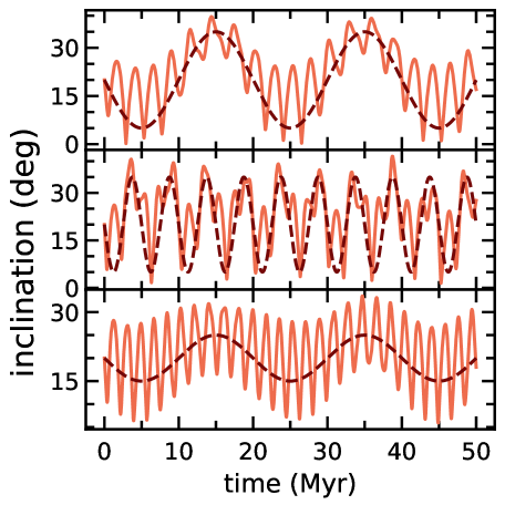
Figure 3: Fifty million year evolution of Neptune’s inclination for three different simulations initialized as described by column one in Table 2 except Neptune’s inclination is $20^{\circ}$. We artificially evolve Neptune’s inclination as a sinusoid, varying $\Delta i$ and $\tau_{i}$ relative to the secular amplitude, $\mathcal{A}_{\rm sec}$ and oscillation timescale, $\tau_{\rm sec}$ with three examples: (1) $\Delta i>\mathcal{A}_{\rm sec}$ and $\tau_{i}>\tau_{\rm sec}$ (top panel), (2) $\Delta i>\mathcal{A}_{\rm sec}$ and $\tau_{i}<\tau_{\rm sec}$ (middle panel), and (3) $\Delta i<\mathcal{A}_{\rm sec}$ and $\tau_{i}>\tau_{\rm sec}$ (bottom panel).

The artificial evolution of $\omega$ and $\Omega$ in a multi-planet case requires a more careful consideration than that of the other elements. One cannot choose completely arbitrary functions for their evolution because the interactions between the planets dominate many attempts to control them. If planets are not strongly coupled, then the phase angles will be easier to force, but this is typically not the case in a multi-planet system. For example, for several test simulations with Jupiter and Neptune, we added and subtracted a small amount of precession to Jupiter by imposing a linear evolution on top of the $\Omega_{J}$. This is helpful if one desires to slow down or speed up the precession of a planet. In these simulations, Neptune’s $\Omega_{N}$ also increased or decreased, respectively, such that $\Omega_{J}-\Omega_{N}$ remained constant. In another test (not shown), we increased $\Omega_{J}$ and decreased $\Omega_{N}$ so that $\Omega_{J}-\Omega_{N}$ changed over time. For this test, the amplitude and frequency of the eccentricity and inclination varied over time in combination with the change of $\Omega_{J}-\Omega_{N}$, thus changing the secular structure. One example of increasing Jupiter’s $\omega_{J}$ is shown in Figure 4. Ficticious evolution of the phase angles is worth considering for scenarios where the user is interested in altering the interactions between the planets, for example in order to track how varying precession affects thousands of particles in the disk. We discuss these implications further in Section 5.

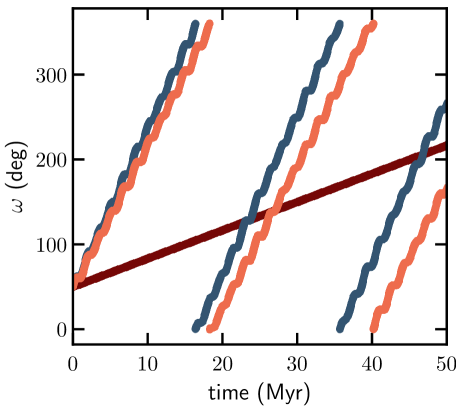
Figure 4: Fifty million year evolution of Jupiter’s $\omega$ (orange) under the gravitational influence of a solar-mass star and Neptune-mass planet. This simulation is initialized with the parameters described in column one of Table 2. In another simulation, we add a linear perturbation over time to Jupiter’s $\omega$ (maroon line), making Jupiter precess faster (blue line).

4 Applications for Artificial Planetary Evolution

Here we show appropriate applications for which to use this code. In planetary instability models (e.g. Tsiganis et al., 2005; Levison et al., 2008, 2011; Nesvorný, 2018; de Sousa et al., 2020), the rearrangement and migration of the outer Solar System planets is typically ignited by Jupiter and Saturn crossing or exiting from a mutual mean motion resonance, which causes their orbital eccentricities to be excited. The resulting planetary instability excites the orbits of the other giant planets, and they undergo a chaotic era of strong planet-planet interactions for several millions to tens of millions of years. In simulations with successful outcomes that qualitatively match the real solar system, Uranus and Neptune, characterized by their eccentric and inclined orbits, are typically damped to more circular and coplanar orbits by dynamical friction (i.e. exchange of angular momentum and energy between the planets and nearby planetesimals). At this time, Jupiter and Saturn were most likely damped to some extent as well but not as much as the outer ice giants. The details of when an instability occurred and how long or how far Neptune migrated remain uncertain. The unprecedented outer solar system de-biased survey made by the Vera C. Rubin Observatory Legacy Survey of Space and Time will help constrain the giant planets evolution even further by allowing comparisons betweeen simulations and observations. In the context of instability models, we can split the possible story of the outer solar evolution into two phases: a chaotic phase and a damping (and migration, though we focus on eccentricity damping) phase.

The behavior of the planets in the chaotic era is unpredictable. Simulations with minuscule changes in the initial conditions of a planetary system produce vastly different planetary behaviors and outcomes. The original planetary instability model (the Nice model—Tsiganis et al. (2005)) included a fifth giant planet that was expelled from the system, and the two farthest planets switched locations in a fraction of simulations. The stochasticity of planet behaviors for various initial conditions makes statistical validation of the initial conditions and outcomes challenging. In addition, massive planetesimals are necessary in the simulation for two important aspects of this model: (1) instigating the initial mean motion resonance crossing between Jupiter and Saturn that leads to an instability and (2) damping Uranus’ and Neptune’s eccentricity which facilitates a stable configuration after tens of millions of years. Including massive planetesimals in such a simulation, makes this a more computationally expensive problem. The interactions between the planets and planetesimals causes the simulations to run for a longer amount of time and adds an extra layer of chaos. To mitigate this complication, artificial forces—as discussed in this paper—can be used to mimic the presence of a massive planetesimal disk and artificially evolve planets’ orbits.

In this section we show two example applications of artificial planet evolution: (1) reproducing phases of migration and eccentricity damping after a planetary instability and (2) investigating the secular coupling between Uranus and Neptune by artificially damping Neptune’s eccentricity and seeing the effect on Uranus’ eccentricity. For both applications, our initial conditions are set by the planet parameters after a chaotic evolution/before a migration from the simulation described in Figure 1 of Tsiganis et al. (2005).

4.1 Reproducing Epochs of Migration and Eccentricity Damping

Reproducing epochs of migration and eccentricity damping after an instability phase is important for studying how the small bodies in the outer solar system—TNOs in mean motion resonance, in particular—are affected by various types of planet evolutions post-instability. In this paper we focus on reproducing the planet evolution and apply this to TNO populations in future work. We aim to reproduce two smooth migration and eccentricity damping phases of Uranus and Neptune in the well-known planet instability model from Tsiganis et al. (2005) to show the usage of this code. We note that it is now well understood that the simulation in Tsiganis et al. (2005) was not able to reproduce all aspects of the planets’ orbits. We use it here as a test-case for validation of our code because it has been well studied.

We extrapolate the eccentricity evolution of the giant planets from Figure 1 in Tsiganis et al. (2005) using the semi-major axis, apocenter, and pericenter curves. We calculate "early" and "late" eccentricity time-evolution profiles for Uranus and Neptune using the values in the three curves since $a_{\rm peri}=a(1-e)$ and $a_{\rm apo}=a(1+e)$. (See Figure 5). We fit an exponential function $\Delta e+e_{0}+\Delta e\exp{t/\tau}$ to the data to find a best-fit damping timescale, $\tau$. The presence of a massive planetesimal disk in Tsiganis et al. (2005) simulations is responsible for damping the eccentricities of Uranus and Neptune. After millions of years, the volume density of the disk can drop by 2-3 orders of magnitude, so the damping rate decreases as well. Our goal here is to calculate damping timescales due to analytical dynamical friction theory and compare with the best fit damping timescales extracted from the simulations to confirm dynamical friction is the dominant force at play. With this example, we will demonstrate how one can artificially evolve planets according to a physically motivated process.

To calculate an eccentricity damping timescale due to dynamical friction we use the parameters of the disk stated in Tsiganis et al. (2005) and in the caption of their Figure 1. The information that is not explicitly stated is assumed to the best of our ability and does not impact the timescale substantially. The initial orbits of Jupiter, Saturn, Uranus, and Neptune are nearly circular and coplanar ($e\sim i\sim 0.001$) with initial semimajor axes 5.45, 8.65, 17, and $\sim$11, respectively. In that simulation, Uranus and Neptune switch orbital positions, a phenomenon that occurred $\sim 50$% of the time. Their simulated planetesimal disk is 35 $M_{\rm E}$, composed of 3500 equal-mass particles up to 30 au, and has a surface density that falls linearly with heliocentric distance. We assume an inner edge of 17 au, since it is not stated in the paper. All particles are initialized with ($e\approx\sin i\approx 0.05$). These values are essential in calculating the timescale at which Neptune would damp due to dynamical friction, since the amount of momentum exchange between the planets and the planetesimals in the disk depends on the volume density of the medium.

Encounters between the planet and sea of planetesimals changes the relative velocity between the two bodies, which is the difference between the orbital velocity of the planet and mean disk flow. The relative velocity can be dominated by the planet’s or planetesimal’s random velocity, which we define as $v^{2}=v_{l}^{2}+v_{P}^{2}$, where $v_{l}$ is the planetesimal’s random velocity and $v_{P}$ is the planet’s random velocity. The order of magnitude momentum exchange of the encounter per time is given by $M_{P}\frac{dv}{dt}=-(mv)n\sigma v_{=}-\rho\sigma v^{2}$, where $M_{P}$ is the mass of the planet, $m$ is the mass of an individual planetesimal, $\rho$ is the volume density of the disk, $\sigma$ is the cross section area for the encounter. Assuming the strong scattering cross section determined by the impact parameter $b\approx GM_{P}/v^{2}$, the equation simplifies to $M_{P}\frac{dv}{dt}=-\rho\Big{(}\frac{GM_{P}}{v^{2}}\Big{)}^{2}v^{2}$. This form matches that found in Goldreich et al. (2004) and Ford & Chiang (2007), which we follow for a portion of this calculation. We adopt constants that were dropped in the order of magnitude expression moving forward. The dynamical friction force is thus given by

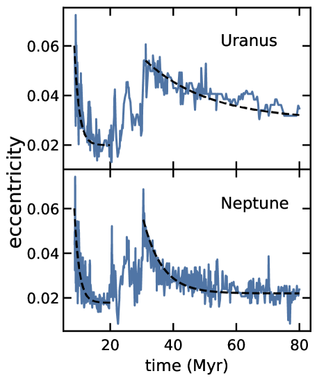
Figure 5: Eccentricity for Uranus (top panel) and Neptune (bottom panel) calculated by using the semimajor axis, pericenter, and apocenter curves from Figure 1 of Tsiganis et al. (2005). The best-fit exponential damping timescale at the early stage (before 20 Myr) is 1.5 Myr for both Uranus and Neptune. At late times (after 30 Myr), the best-fit exponential timescales are 20 Myr and 6 Myr for Uranus and Neptune, respectively (see Section 4.1).

$$\frac{dv}{dt}=-\frac{2\pi G^{2}M_{P}\rho}{v^{2}}\ln(1+\Lambda^{2})$$ (8)

where the Coloumb parameter, $\Lambda$ is

$$\Lambda=b_{\rm max}\big{(}v^{2}+2\langle\sin(i_{l})^{2}\rangle v_{\rm circ}^{2}\big{)}\Big{/}(GM_{P})$$ (9)

and

$$b_{\rm max}=R_{H}+r\big{(}\langle\sin(i_{l})^{2}\rangle+\sin(i_{P})^{2}\big{)}^{1/2}$$ (10)

The subscripts $l$ and $P$ represent the planetesimal and planet, respectively. The calculation in Ford & Chiang (2007) assumes the planet interacts with the disk twice since they assume $i_{P}\gg i_{l}$, whereas we are assuming that the planet and planetesimal disk have similar inclinations (i.e. the planet is embedded in the disk and feels the perturbation on behalf of the disk for the duration of an orbital period). The change in planet’s velocity due to the interactions with the planetsimals is $\Delta v_{P}$ and the interaction time, $\Delta t$, is the orbital period, $2\pi/\Omega$. The kicks thus produce $\Delta v_{P}\approx\frac{dv}{dt}\Delta t$, so that

$$\frac{dv_{P}}{dt}=\frac{\Delta v_{P}}{t_{\rm orb}}=-\frac{2\pi G^{2}M_{P}}{v^{2}}\ln(1+\Lambda^{2})\rho$$ (11)

$$\frac{de_{P}}{dt}a\Omega\hat{\boldsymbol{p}}=-\frac{2\pi G^{2}M_{P}}{(\sqrt{2}e_{P}a\Omega)v^{2}}\ln(1+\Lambda^{2})\rho(e_{P}a\Omega\hat{\boldsymbol{p}}+i_{P}a\Omega\hat{\boldsymbol{z}})$$ (12)

$$\frac{de_{P}}{dt}=-\frac{\pi}{\sqrt{2}}\frac{G}{\Omega}\frac{M_{P}}{M_{*}}\ln(1+\Lambda^{2})\frac{\Sigma}{H}\frac{1}{e_{l}^{2}+e_{P}^{2}}$$ (13)

$$t_{\rm damp}=\frac{e_{P}}{de_{P}/dt}$$ (14)

Plugging in the appropriate disk and Neptune parameters from Tsiganis et al. (2005) simulation and scaling the mass volume density of the disk due to the dispersal after millions of years, we calculate one million years and eight million years for Neptune’s early and late damping phases, respectively. These values match the damping timescales from the simulation (see Figure 5). The physical process of dynamical friction is responsible for damping Neptune’s eccentricity in the simulation, and it turns out to be well-represented by an exponential function with an order of magnitude estimated timescale.

We confirm the appropriate use of an exponential function representing the dynamical friction process due to interactions between the planets and massive planetesimals. We use the best-fit values to initialize simulations of the giant planets with migration and eccentricity damping parameters. In Figure 6 we show a simulation where we successfully reproduce early and late epochs of outward migration (top panel) and eccentricity damping for Uranus (middle panel) and Neptune (bottom panel). With this exercise, we show an appropriate use for aritficially evolving planets’ orbits, motivated by a physical process. While for this case, our goal was to reproduce the scenario is a specific simulation, for the case of outer solar system models, the goal is to evolve the giant planets’ orbit such that they match the current observed state of the Solar System. This involves changing the parameters in the functional form describing the evolution. Specifically, the parameters to change are the scale of the change and the timescale of the change (see Equation 7).

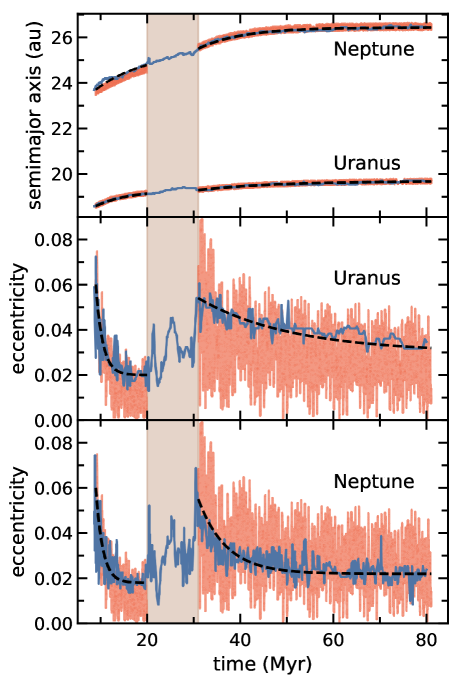
Figure 6: Two example simulations (orange) showing the evolution of the semimajor axes (top panel) and eccentricities of Uranus (middle panel) and Neptune (bottom panel) representing an early and late damping phase (separated by the shaded region). We artificially evolve the two outer planets’ orbits using the best-fit parameters from Figure 5. The evolution from Figure 5 is shown for reference in blue. The dashed curves show the best fit exponential evolution for each early and late migration/damping phase. We note that because this is a chaotic problem, slightly different initial conditions produce vastly different results. Simply randomizing the initial phase angles from 0 to $2\pi$ for an ensemble of 40 simulations produced $\approx$ 20 simulations with completely different final outcomes.

4.2 Effect of Damping Neptune on Uranus

An interesting outcome of our code tests is that of isolating the impact of exclusively damping Neptune’s eccentricity as if it had been damped by dynamical friction. With this method, we study how the secular coupling between Uranus and Neptune at early and late stages affects the evolution of Uranus. This effect is similar to the redistribution of tidal damping by secular coupling between planets (Greenberg et al., 2013). By modeling Neptune’s evolution artificially and without a massive planetesimal disk, we can study the interactions between Uranus and Neptune in isolation.

We find that as Neptune’s eccentricity damps, Neptune exerts a force on Uranus, such that Uranus’ eccentricity damps as well. The magnitude of the effect depends on a few parameters. If Neptune’s damping timescale is short ($\la$ 1 Myr) or the change in eccentricity is small ($\la$ 0.01), then the effect on Uranus is negligible. Figure 7 shows a simulation that is initialized in the same way as that described in Figure 6 for the late phase, but only Neptune’s eccentricity and semimajor axis are evolved (bottom panels; dark maroon lines). Uranus’ eccentricity is indirectly damped in this simulation through interactions with Neptune (top right panel). The dashed line over the simulation data (top right panel) is the same dashed line from Uranus’ late migration in Figure 6 (middle panel). This shows that only damping Neptune’s eccentricity is sufficient to damp Uranus’ eccentricity, without the need of dynamical friction due to interactions with the planetesimal disk. We carried out the same test but for the early phase described in Figure 6 and saw no effect on Uranus (plot not shown). The damping timescale is too short at this early phase (i.e., it is comparable to and shorter than the secular frequency of Uranus and Neptune, respectively), so Neptune’s eccentricity damping does not indirectly damp Uranus.

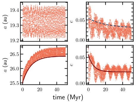
Figure 7: Fifty million year simulation initialized with the same parameters as those in the late stage evolution from Figure 6 and only showing Uranus (top row) and Neptune (bottom row). Neptune’s eccentricity is damped artificially with the functional form shown in dark maroon (bottom middle panel). Uranus’ is not artificially damped in this simulation, rather, it is indirectly damped (top middle panel). The dashed line shows the same damping timescale for Uranus as in Figure 6 to show that the indirect damping of Uranus is comparable to that calculated from Tsiganis et al. (2005).

We run additional simulations similar to those shown in Figure 7, but we vary the initial eccentricity of Neptune and Uranus to investigate how changing the $\Delta e$ will affect the indirect damping on Uranus. Increasing the initial eccentricity of both Uranus and Neptune to a higher value and damping Neptune with the same timescale of 6 million years, results in Uranus’ eccentricity damping to a higher degree (not shown). This effect is interesting to follow up on when studying the late stages of planetary evolution in our solar system. The secular eccentricity timescales of Uranus and Neptune are 0.5 Myr and 2 Myr, therefore the secular coupling between Uranus and Neptune, that would cause Neptune to damp Uranus’ eccentricity indirectly, is stronger at late times when the damping timescale is $\ga 6$ Myr.

While the giant planet instability model has reproduced a vast amount of currently observed structure within the giant planets and Trans-Neptunian Objects, the evolution in between an instability and the current TNO configuration remains unknown. This includes the possibility that Uranus and Neptune were launched onto orbits with eccentricities as high as 0.4 and damped at various magnitudes and rates depending on the volume density of the planetesimal disk. With this in mind, we run a last suite of simulations similar to those described in Figure 7 with Uranus’ eccentricity initialized at values higher than Neptune’s. One such example is shown in Figure 8. In this simulation, Uranus’ and Neptune’s eccentricity are initialized at 0.1 and 0.065, respectively, representing a scenario just before a damping phase. Both planets are artificially damped with the same eccentricity-damping timescale, motivated by instability simulations that show the number density near Uranus and Neptune is comparable after a few million years post-instability (not shown). We find that Neptune’s effect on Uranus is significant enough to damp Uranus’ eccentricity by a larger amount than what we prescribed (top middle panel). The secular coupling between Uranus and Neptune at this late stage of evolution is important to understand in order to constrain how dynamical friction sets the final eccentricities of the ice giants.

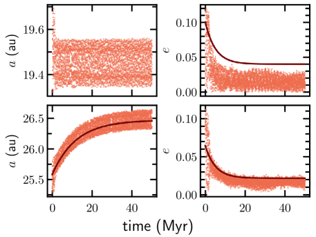
Figure 8: Fifty million year simulation initialized with the same parameters as those in the late stage evolution from Figure 6, except Uranus (top row) and Neptune (bottom row) start at eccentricities 0.1 and 0.065, respectively. Both planets are artificially damped with the same timescale of 5 Myr. Uranus’ eccentricity damps further than the amount we prescribe (top middle panel) due to the secular effects with Neptune.

4.3 Discussion of Future Applications

In this paper we focus on Uranus’ and Neptune’s artificial orbital evolution in the context of reproducing migration/eccentricity damping phases in a well-known planetary instability simulation and isolating the impact of one planet’s eccentricity damping in the absence of a planetesimal disk. Artificial evolution is also useful for outer solar system studies that probe how different giant planet dynamical histories affect the orbital configuration of Trans Neptunian Objects (TNOs). A variety of proposed migration histories within the outer solar system, modeled through numerical simulations, produce different planet and TNO structure (for reveiws see Nesvorný, 2018; Gladman & Volk, 2021). In fact, a similar migration history, with minuscule changes in initial conditions, could also produce vastly distinct planet trajectories as is the case for planetary instability numerical models as discussed in Section 4, where chaos is the underlying driver Volk & Malhotra (2019).

A realistic portrayal of a planetary system in an N-body simulation would require all solar system planets and billions of massive planetesimals. The chaotic nature of this problem is further accentuated by the additional gravitational interactions between each body, making exploration of a large parameter space of initial conditions computationally infeasible. The ability to artificially evolve planets’ orbits is therefore beneficial for investigating how TNOs in mean motion resonance (MMR) with Neptune evolve as a result of various migration histories.

5 Summary

The modifications to REBOUND and Mercury6.2 we present in this paper are essential for running suites of N-body simulations that can probe a large parameter space of orbital configurations for the purpose of constraining the evolution of the outer solar system. We demonstrate how to evolve particles’ orbital evolutions with arbitrary functions using our modifications. We show that with a one-planet simulation, all orbital elements can be evolved independently from each other. Introducing a second planet to the system, adds new gravitational interactions between the planets, which affects the amount of control one has over the artificial evolution of each orbital element. Secular perturbations between the planets produce oscillations in eccentricity and inclination. It is important to consider how the secular frequencies and amplitudes of the planets compare to the desired scale of change and timescale of change to successfully evolve these elements accordingly.

We demonstrate two appropriate uses of this code, emphasizing the need for physically motivated functional forms for a given orbital evolution. In our case, we used the planetary instability simulation in Tsiganis et al. (2005) to validate the use of our code and artificially evolve the semimajor axis and eccentricity of Uranus and Neptune. We choose an exponential function to evolve these parameters and confirm migration/damping timescales with dynamical friction derivations appropriate for the planetesimal disk in their simulation. We are able to reproduce two stages of migration and eccentricity damping, which we call the early and late stages. This result is important for studying various migration scenarios post-instability and how that affects the orbital distribution of trans-neptunian objects. Lastly, we find that artificially damping Neptune’s eccentricity indirectly damps Uranus’ eccentricity due to their secular coupling. At late stages of evolution, coupling between the latter two planets is important to consider since the planetesimal disk will have dissipated significantly.

Data Availability

REBOUND code, and example scripts to create the figures from this paper are available on my github: https://github.com/ahermosillo. Simulation data is available upon request.

Appendix A Modifications to the equations of motion

We modify two N-body integration codes, Mercury 6.2 and REBOUND, and confirm that we reproduce the same planetary evolution when applying the same orbital evolution functional forms to identical planetary initial conditions.

Modifications to Mercury 6.2 in the way we are using them, were done by Dawson & Murray-Clay (2012) and Wolff et al. (2012) and are described in the Appendix of Wolff et al. (2012). We reiterate those modifications in this section with specifics and discuss additional modifications to the equations of motions to allow for artificial evolution of the phase angles argument of pericenter and longitude of ascending node. Modifications to REBOUND are explained below as well. We note that these modifications are non-symplectic, even for a symplectic integrator, thus, the modifications must represent small perturbations on the planet for this to be valid. These modifications were tested for the MVS and HYBRID integrators within Mercury and for the WHFAST and MERCURIUS integrators within REBOUND; the tests were run for systems with a star and 1, 2, or 4 planets.

The modifications in REBOUND are made as follows:

• In rebound.h, we created six new members for the structure reb_particle: vusrx, vusry, vusrz, ausrx, ausry, ausrz. As is default for the other members in the structure, these user velocity and acceleration terms are initialized to nan or zero in particle.c and tools.c.

• As is default in REBOUND, to turn on extra forces in the simulation, sim->additionalforces must be set to the name of a user-defined function that defines the additional forces on the desired particles. In our case, this function is setting both additional forces and velocities, since this is where we add the user velocity and acceleration terms mentioned in bullet one, defined by Equations (5). For example, in sim->additionalforces=migrationforce, inside the function migrationforce, the user velocity for a given particle, referenced by p, is set by: p->vusrx += dxda*adot + dxde*edot + dxdi*idot + dxdom*omdot + dxdOm*Omdot.

• The integration of the motion of particles is typically split up into a few components depending on the type of interactions one is interested in modeling. The update goes in the interaction step (Mercurius goes through interaction step, jump step,kepler step,jump step, and one final interaction step if the coordinates are not synchronized. Each individual step updates the position and velocity of each particle.) By default, the function reb_integrator_mercurius_interaction_step in integrator_mercurius.c, only updates the velocity of the particle with the acceleration. When the additionalforces attribute is turned on, the acceleration includes the additional force. In our case, the user defined force is its own variable: ausrx, ausry, ausrz. We modified the function reb_integrator_mercurius_interaction_step to update the position and velocity of the particle using the additional velocity and acceleration. Specifically, the velocity of the particle is updated with ax as is the default. Then we transform the coordinates from democratic heliocentric coordinates to intertial using reb_integrator_mercurius_dh_to_inertial(r) to update the position and velocities using the user defined variables like:

  particles[i].vx += dt*particles[i].ausrx particles[i].x += dt*particles[i].vusrx.

  Then, we tranform the coordinates back to democratic heliocentric with reb_integrator_mercurius_inertial_to_dh(r);

• Lastly, with the addition of the new attributes to the particles struct, the simulation archive needed significant changes.

The modifications in Mercury6.2 are made as follows:

• As is default in Mercury6.2, the velocity of an object is updated in the interaction step of a given integrator algorithm. In MDT_HY.FOR, we modify the interaction step portions (there are two of them) to update the position of the particle as well with the user-defined velocity like x(1,j) = x(1,j) + hby2 * vusr(1,j) where hby2 is half a time-step. An equivalent line of code is written for the $y$ and $z$ coordinates. In this same routine, we initialize the vusr vector at the beginning.

• The MFO_USER.FOR routine is modified to return a user-defined velocity in addition to the already supported, user-defined acceleration. This routine calculates the user-defined velocity and acceleration terms from Equation 1 and applies them to the planets the user desires. Here, we initialize the $\Delta$ values that are part of the $\dot{a}$, $\dot{e}$, etc and so on.

To derive the additional terms, we allow all orbital elements to vary with time and define them to be independent from each other. The position vector components ($x$,$y$,$z$) are given in equation 3, as a function of the orbital elements. The variable $r$ is the distance of the planet from the central body, $\Omega$ is the longitude of ascending node in the xy plane, $\omega$ is the arguments of periapse, $f$ is the true anamoly, and $i$ is the inclination.

$$x=r\cos{\Omega}\cos{(\omega+f)}-r\cos{i}\sin{\Omega}\sin{(\omega+f)}$$ (15)

$$y=r\sin{\Omega}\cos{(\omega+f)}+r\cos{i}\cos{\Omega}\sin{(\omega+f)}$$ (16)

$$z=r\sin{i}\sin{(\omega+f)}$$ (17)

The velocity vetctor componenets are given by ($\dot{x}$, $\dot{y}$, and $\dot{z}$)

$$\dot{x} =\dot{r}\cos{\Omega}\cos{(\omega+f)}-r\sin{\Omega}\dot{\Omega}\cos{(\omega+f)}$$ (18)

$$-(r\dot{\omega}+r\dot{f})\cos{\Omega}\sin{(\omega+f)}-\dot{r}\cos{i}\sin{\Omega}\sin{(\omega+f)}$$

$$+r\sin{i}\dot{I}\sin{\Omega}\sin{(\omega+f)}-r\cos{i}\cos{\Omega}\dot{\Omega}\sin{(\omega+f)}$$

$$-(r\dot{\omega}+r\dot{f})\cos{i}\sin{\Omega}\cos{(\omega+f)}$$

$$\dot{y} =\dot{r}\sin{\Omega}\cos{(\omega+f)}+r\cos{\Omega}\dot{\Omega}\cos{(\omega+f)}$$ (19)

$$-(r\dot{\omega}+r\dot{f})\sin{\Omega}\sin{(\omega+f)}+\dot{r}\cos{i}\cos{\Omega}\sin{(\omega+f)}$$

$$-r\sin{i}\dot{I}\cos{\Omega}\sin{(\omega+f)}-r\cos{i}\sin{\Omega}\dot{\Omega}\sin{(\omega+f)}$$

$$+(r\dot{\omega}+r\dot{f})\cos{i}\cos{\Omega}\cos{(\omega+f)}$$

$$\dot{z} =\dot{r}\sin{i}\sin{(\omega+f)}+r\cos{i}\dot{I}\sin{(\omega+f)}$$ (20)

$$+(r\dot{w}+r\dot{f})\sin{i}\cos{(\omega+f)}$$

The ficticious x-component "velocity" and "acceleration" used to update the planets’ position and velocity in MERCURY are given by:

$$\large\dot{x}=\frac{dx}{dt}=\frac{\partial x}{\partial a}\dot{a}+\frac{\partial x}{\partial e}\dot{e}+\frac{\partial x}{\partial i}\dot{i}+\frac{\partial x}{\partial\omega}\dot{\omega}+\frac{\partial x}{\partial\Omega}\dot{\Omega}+\frac{\partial x}{\partial f}\dot{f}$$ (21)

$$\large\ddot{x}=\frac{d\dot{x}}{dt}=\frac{\partial\dot{x}}{\partial a}\dot{a}+\frac{\partial\dot{x}}{\partial e}\dot{e}+\frac{\partial\dot{x}}{\partial i}\dot{i}+\frac{\partial\dot{x}}{\partial\omega}\dot{\omega}+\frac{\partial\dot{x}}{\partial\Omega}\dot{\Omega}+\frac{\partial\dot{x}}{\partial f}\dot{f}$$ (22)

where similar expressions are derived for the other coordinates. These equations do not describe the entire evolution of the planets; they are additional terms due to their orbital element evolution. In MERCURY, these are added onto the existing acceleration and velocity terms in the code. Note that we do not include the $\dot{f}$ term since that is inherent to the Keplerian motion of the planet, and we do not update that value. These partial derivatives include $r$, $\dot{r}$, $r\dot{f}$ and their derivatives w.r.t. $a$,$e$, $f$:

$$r=\frac{a(1-e^{2})}{1+e\cos{f}}$$ (23)

$$r\dot{f}=\sqrt{\frac{M}{a}}\frac{1+e\cos{f}}{\sqrt{1-e^{2}}}$$ (24)

$$\dot{r}=\frac{\partial r}{\partial a}\dot{a}+\frac{\partial r}{\partial e}\dot{e}+\frac{\partial r}{\partial f}\dot{f}$$ (25)

$$\dot{f}=\frac{r\dot{f}}{r}=\sqrt{\frac{M}{a^{3}}}\frac{(1+e\cos{f})^{2}}{(1-e^{2})^{3/2}}$$ (26)

$$\frac{\partial r}{\partial a}=\frac{1-e^{2}}{1+e\cos{f}}=\frac{r}{a}$$ (27)

$$\frac{\partial r}{\partial e}=-\frac{2ae}{1+e\cos{f}}-\frac{a(1-e^{2})\cos{f}}{(1+e\cos{f})^{2}}$$ (28)

$$\frac{\partial r}{\partial f}=\frac{a(1-e^{2})e\sin{f}}{(1+e\cos{f})^{2}}$$ (29)

$$\frac{\partial r\dot{f}}{\partial a}=\frac{-r\dot{f}}{2a}=-\frac{1}{2}\sqrt{\frac{M}{a^{3}}}\frac{1+e\cos{f}}{\sqrt{1-e^{2}}}$$ (30)

$$\frac{\partial r\dot{f}}{\partial e}=\frac{r\dot{f}(e+\cos{f})}{(1-e^{2})(1+e\cos{f})}=\sqrt{\frac{M}{a}}\frac{e+e\cos{f}}{(1-e^{2})^{3/2}}$$ (31)

$$\frac{\partial r\dot{f}}{\partial f}=\frac{-a\sqrt{M/a^{3}}e\sin{f}}{\sqrt{1-e^{2}}}$$ (32)

$$\frac{\partial\dot{f}}{\partial a}=-3/2\frac{\sqrt{M/a^{5}}(1+e\cos{f})^{2}}{(1-e^{2})^{3/2}}$$ (33)

$$\frac{\partial\dot{f}}{\partial e}=\sqrt{\frac{M}{a^{3}}}\Big{(}\frac{2(1+e\cos{f})\cos{f}}{(1-e^{2})^{3/2}}+\frac{3e(1+e\cos{f})^{2}}{(1-e^{2})^{5/2}}\Big{)}$$ (34)

$$\frac{\partial\dot{f}}{\partial f}=-\frac{2\sqrt{M/a^{3}}(1+e\cos{f})e\sin{f}}{(1-e^{2})^{3/2}}$$ (35)

$$\frac{\partial\dot{r}}{\partial a} =\Big{(}\frac{-2e}{1+e\cos{f}}-\frac{(1-e^{2})\cos{f}}{(1+e\cos{f})^{2}}\Big{)}\dot{e}$$ (36)

$$+\Big{(}\frac{(1-e^{2})e\sin{f}}{(1+e\cos{f})^{2}}\Big{)}\dot{f}+\frac{a(1-e^{2})e\sin{f}}{(1+e\cos{f})^{2}}\frac{\partial\dot{f}}{\partial a}$$

$$\frac{\partial\dot{r}}{\partial e} =\Big{(}\frac{-2e}{1+e\cos{f}}-\frac{(1-e^{2})\cos{f}}{(1+e\cos{f})^{2}}\Big{)}\dot{a}$$ (37)

$$+\Big{(}\frac{-2a}{(1+e\cos{f})}+\frac{4ae\cos{f}}{(1+e\cos{f})^{2}}+\frac{2a(1-e^{2})(\cos{f})^{2}}{(1+e\cos{f})^{3}}\Big{)}\dot{e}$$

$$+\Big{(}\frac{a(1-3e^{2})\sin{f}}{(1+e\cos{f})^{2}}-\frac{2a(e-e^{3})\sin{f}\cos{f}}{(1+e\cos{f})^{3}}\Big{)}\dot{f}$$

$$+\Big{(}\frac{a(1-e^{2})e\sin{f}}{(1+e\cos{f})^{2}}\Big{)}\frac{\partial\dot{f}}{\partial e}$$

$$\frac{\partial\dot{r}}{\partial f} =\frac{(1-e^{2})e\sin{f}}{(1+e\cos{f})^{2}}\dot{a}$$ (38)

$$+\Big{(}\frac{-2ae^{2}\sin{f}}{(1+e\cos{f})^{2}}+\frac{a(1-e^{2})\sin{f}}{(1+e\cos{f})^{2}}-\frac{-2a(1-e^{2})\cos{f}e\sin{f}}{(1+e\cos{f})^{3}}\Big{)}\dot{e}$$

$$+\Big{(}\frac{a(1-e^{2})e\cos{f}}{(1+e\cos{f})^{2}}+\frac{2a(1-e^{2})e^{2}\sin{f}^{2}}{(1+e\cos{f})^{3}}\Big{)}\dot{f}$$

$$+\Big{(}\frac{a(1-e^{2})e\sin{f}}{(1+e\cos{f})^{2}}\Big{)}\frac{\partial\dot{f}}{\partial f}$$ (39)

The terms found in equations 21 and 22 are given by

$$\frac{\partial x}{\partial a}=\frac{\partial r}{\partial a}\cos{\Omega}\cos{(\omega+f)}-\frac{\partial r}{\partial a}\cos{i}\sin{\Omega}\sin{(\omega+f)}$$ (40)

$$\frac{\partial x}{\partial e}=\frac{\partial r}{\partial e}\cos{\Omega}\cos{(\omega+f)}-\frac{\partial r}{\partial e}\cos{i}\sin{\Omega}\sin{(\omega+f)}$$ (41)

$$\frac{\partial x}{\partial i}=r\sin{i}\sin{\Omega}\sin{(\omega+f)}$$ (42)

$$\frac{\partial x}{\partial\Omega}=-r\sin{\Omega}\cos{(\omega+f)}-r\cos{i}\cos{\Omega}\sin{(\omega+f)}$$ (43)

$$\frac{\partial x}{\partial\omega}=-r\cos{\Omega}\sin{(\omega+f)}-r\cos{i}\sin{\Omega}\cos{(\omega+f)}$$ (44)

$$\frac{\partial x}{\partial f} =\frac{\partial r}{\partial f}\cos{\Omega}\cos{(\omega+f)}-r\cos{\Omega}\sin{(\omega+f)}$$ (45)

$$-\frac{\partial r}{\partial f}\cos{i}\sin{\Omega}\sin{(\omega+f)}-r\cos{i}\sin{\Omega}\cos{(\omega+f)}$$

$$\frac{\partial y}{\partial a}=\frac{\partial r}{\partial a}\sin{\Omega}\cos{(\omega+f)}+\frac{\partial r}{\partial a}\cos{i}\cos{\Omega}\sin{(\omega+f)}$$ (46)

$$\frac{\partial y}{\partial e}=\frac{\partial r}{\partial e}\sin{\Omega}\cos{(\omega+f)}+\frac{\partial r}{\partial e}\cos{i}\cos{\Omega}\sin{(\omega+f)}$$ (47)

$$\frac{\partial y}{\partial i}=-r\sin{i}\cos{\Omega}\sin{(\omega+f)}$$ (48)

$$\frac{\partial y}{\partial\Omega}=r\cos{\Omega}\cos{(\omega+f)}-r\cos{i}\sin{\Omega}\sin{(\omega+f)}$$ (49)

$$\frac{\partial y}{\partial\omega}=-r\sin{\Omega}\sin{(\omega+f)}+r\cos{i}\cos{\Omega}\cos{(\omega+f)}$$ (50)

$$\frac{\partial y}{\partial f} =\frac{\partial r}{\partial f}\sin{\Omega}\cos{(\omega+f)}-r\sin{\Omega}\sin{(\omega+f)}$$ (51)

$$+\frac{\partial r}{\partial f}\cos{i}\cos{\Omega}\sin{(\omega+f)}+r\cos{i}\cos{\Omega}\cos{(\omega+f)}$$

$$\frac{\partial z}{\partial a}=\frac{\partial r}{\partial a}\sin{i}\sin{(\omega+f)}$$ (52)

$$\frac{\partial z}{\partial e}=\frac{\partial r}{\partial e}\sin{i}\sin{(\omega+f)}$$ (53)

$$\frac{\partial z}{\partial i}=r\cos{i}\sin{(\omega+f)}$$ (54)

$$\frac{\partial z}{\partial\Omega}=0.0$$ (55)

$$\frac{\partial z}{\partial\omega}=r\sin{i}\cos{(\omega+f)}$$ (56)

$$\frac{\partial z}{\partial f}=\frac{\partial r}{\partial f}\sin{i}\sin{(\omega+f)}+r\sin{i}\cos{(\omega+f)}$$ (57)

$$\frac{\partial\dot{x}}{\partial a} =\frac{\partial\dot{r}}{\partial a}\cos{(\Omega)}\cos{(\omega+f)}-\frac{\partial r}{\partial a}\sin{\Omega}\dot{\Omega}\cos{(\omega+f)}$$ (58)

$$-(\frac{\partial r}{\partial a}\dot{\omega}+\frac{\partial r\dot{f}}{\partial a})\cos{\Omega}\sin{(\omega+f)}-\frac{\partial\dot{r}}{\partial a}\cos{i}\sin{\Omega}\sin{(\omega+f)}$$

$$+\frac{\partial r}{\partial a}\sin{i}\dot{I}\sin{\Omega}\sin{(\omega+f)}-\frac{\partial r}{\partial a}\cos{i}\cos{\Omega}\dot{\Omega}\sin{(\omega+f)}$$

$$-(\frac{\partial r}{\partial a}\dot{\omega}+\frac{\partial r\dot{f}}{\partial a})\cos{i}\sin{\Omega}\cos{(\omega+f)}$$

$$\frac{\partial\dot{x}}{\partial e} =\frac{\partial\dot{r}}{\partial e}\cos{\Omega}\cos{(\omega+f)}-\frac{\partial r}{\partial e}\sin{\Omega}\dot{\Omega}\cos{(\omega+f)}$$ (59)

$$-(\frac{\partial r}{\partial e}\dot{\omega}+\frac{\partial r\dot{f}}{\partial e})\cos{\Omega}\sin{(\omega+f)}-\frac{\partial\dot{r}}{\partial e}\cos{i}\sin{\Omega}\sin{(\omega+f)}$$

$$+\frac{\partial r}{\partial e}\sin{i}\dot{I}\sin{\Omega}\sin{(\omega+f)}-\frac{\partial r}{\partial e}\cos{i}\cos{\Omega}\dot{\Omega}\sin{(\omega+f)}$$

$$-(\frac{\partial r}{\partial e}\dot{\omega}+\frac{\partial r\dot{f}}{\partial e})\cos{i}\sin{\Omega}\cos{(\omega+f)}$$

$$\frac{\partial\dot{x}}{\partial i} =\dot{r}\sin{i}\sin{\Omega}\sin{(\omega+f)}+r\cos{i}\dot{I}\sin{\Omega}\sin{(\omega+f)}$$ (60)

$$+r\sin{i}\cos{\Omega}\dot{\Omega}\sin{(\omega+f)}+(r\dot{\omega}+r\dot{f})\sin{i}\sin{\Omega}\cos{(\omega+f)}$$

$$\frac{\partial\dot{x}}{\partial\Omega} =-\dot{r}\sin{\Omega}\cos{(\omega+f)}-r\cos{\Omega}\dot{\Omega}\cos{(\omega+f)}$$ (61)

$$+(r\dot{\omega}+r\dot{f})\sin{\Omega}\sin{(\omega+f)}-\dot{r}\cos{i}\cos{\Omega}\sin{(\omega+f)}$$

$$+r\sin{i}\dot{I}\cos{\Omega}\sin{(\omega+f)}+r\cos{i}\sin{\Omega}\dot{\Omega}\sin{(\omega+f)}$$

$$-(r\dot{\omega}+r\dot{f})\cos{i}\cos{\Omega}\cos{(\omega+f)}$$

$$\frac{\partial\dot{x}}{\partial\omega} =-\dot{r}\cos{\Omega}\sin{(\omega+f)}+r\sin{\Omega}\dot{\Omega}\sin{(\omega+f)}$$

$$-(r\dot{\omega}+r\dot{f})\cos{\Omega}\cos{(\omega+f)}-\dot{r}\cos{i}\sin{\Omega}\cos{(\omega+f)}$$

$$+r\sin{i}\dot{I}\sin{\Omega}\cos{(\omega+f)}-r\cos{i}\cos{\Omega}\dot{\Omega}\cos{(\omega+f)}$$

$$+(r\dot{\omega}+r\dot{f})\cos{i}\sin{\Omega}\sin{(\omega+f)}$$

$$\frac{\partial\dot{x}}{\partial f} =-\dot{r}\cos{\Omega}\sin{(\omega+f)}+r\sin{\Omega}\dot{\Omega}\sin{(\omega+f)}$$ (62)

$$-(r\dot{\omega}+r\dot{f})\cos{\Omega}\cos{(\omega+f)}-\dot{r}\cos{i}\sin{\Omega}\cos{(\omega+f)}$$

$$+r\sin{i}\dot{I}\sin{\Omega}\cos{(\omega+f)}-r\cos{i}\cos{\Omega}\dot{\Omega}\cos{(\omega+f)}$$

$$+(r\dot{\omega}+r\dot{f})\cos{i}\sin{\Omega}\sin{(\omega+f)}+\frac{\partial\dot{r}}{\partial f}\cos{\Omega}\cos{(\omega+f)}$$

$$-\frac{\partial r}{\partial f}\sin{\Omega}\dot{\Omega}\cos{(\omega+f)}-(\frac{\partial r}{\partial f}\dot{\omega}+\frac{\partial r\dot{f}}{\partial f})\cos{\Omega}\sin{(\omega+f)}$$

$$-\frac{\partial\dot{r}}{\partial f}\cos{i}\sin{\Omega}\sin{(\omega+f)}+\frac{\partial r}{\partial f}\sin{i}\dot{I}\sin{\Omega}\sin{(\omega+f)}$$

$$-\frac{\partial r}{\partial f}\cos{i}\cos{\Omega}\dot{\Omega}\sin{(\omega+f)}-(\frac{\partial r}{\partial f}\dot{\omega}+\frac{\partial r\dot{f}}{\partial f})\cos{i}\sin{\Omega}\cos{(\omega+f)}$$

$$\frac{\partial\dot{y}}{\partial a} =\frac{\partial\dot{r}}{\partial a}\sin{\Omega}\cos{(\omega+f)}+\frac{\partial r}{\partial a}\cos{\Omega}\dot{\Omega}\cos{(\omega+f)}$$ (63)

$$-(\frac{\partial r}{\partial a}\dot{\omega}+\frac{\partial r\dot{f}}{\partial a})\sin{\Omega}\sin{(\omega+f)}+\frac{\partial\dot{r}}{\partial a}\cos{i}\cos{\Omega}\sin{(\omega+f)}$$

$$-\frac{\partial r}{\partial a}\sin{i}\dot{I}\cos{\Omega}\sin{(\omega+f)}-\frac{\partial r}{\partial a}\cos{i}\sin{\Omega}\dot{\Omega}\sin{(\omega+f)}$$

$$+(\frac{\partial r}{\partial a}\dot{\omega}+\frac{\partial r\dot{f}}{\partial a})\cos{i}\cos{\Omega}\cos{(\omega+f)}$$

$$\frac{\partial\dot{y}}{\partial e} =\frac{\partial\dot{r}}{\partial e}\sin{\Omega}\cos{(\omega+f)}+\frac{\partial r}{\partial e}\cos{\Omega}\dot{\Omega}\cos{(\omega+f)}$$ (64)

$$-(\frac{\partial r}{\partial e}\dot{\omega}+\frac{\partial r\dot{f}}{\partial e})\sin{\Omega}\sin{(\omega+f)}+\frac{\partial\dot{r}}{\partial e}\cos{i}\cos{\Omega}\sin{(\omega+f)}$$

$$-\frac{\partial r}{\partial e}\sin{i}\dot{I}\cos{\Omega}\sin{(\omega+f)}-\frac{\partial r}{\partial e}\cos{i}\sin{\Omega}\dot{\Omega}\sin{(\omega+f)}$$

$$+(\frac{\partial r}{\partial e}\dot{\omega}+\frac{\partial r\dot{f}}{\partial e})\cos{i}\cos{\Omega}\cos{(\omega+f)}$$

$$\frac{\partial\dot{y}}{\partial i} =-\dot{r}\sin{i}\cos{\Omega}\sin{(\omega+f)}-r\cos{i}\dot{I}\cos{\Omega}\sin{(\omega+f)}$$ (65)

$$+r\sin{i}\sin{\Omega}\dot{\Omega}\sin{(\omega+f)}-(r\dot{\omega}+r\dot{f})\sin{i}\cos{\Omega}\cos{(\omega+f)}$$

$$\frac{\partial\dot{y}}{\partial\Omega} =\dot{r}\cos{\Omega}\cos{(\omega+f)}-r\sin{\Omega}\dot{\Omega}\cos{(\omega+f)}$$ (66)

$$-(r\dot{\omega}+r\dot{f})\cos{\Omega}\sin{(\omega+f)}-\dot{r}\cos{i}\sin{\Omega}\sin{(\omega+f)}$$

$$+r\sin{i}\dot{I}\sin{\Omega}\sin{(\omega+f)}-r\cos{i}\cos{\Omega}\dot{\Omega}\sin{(\omega+f)}$$

$$-(r\dot{\omega}+r\dot{f})\cos{i}\sin{\Omega}\cos{(\omega+f)}$$

$$\frac{\partial\dot{y}}{\partial\omega} =-\dot{r}\sin{\Omega}\sin{(\omega+f)}-r\cos{\Omega}\dot{\Omega}\sin{(\omega+f)}$$ (67)

$$-(r\dot{\omega}+r\dot{f})\sin{\Omega}\cos{(\omega+f)}+\dot{r}\cos{i}\cos{\Omega}\cos{(\omega+f)}$$

$$-r\sin{i}\dot{I}\cos{\Omega}\cos{(\omega+f)}-r\cos{i}\sin{\Omega}\dot{\Omega}\cos{(\omega+f)}$$

$$-(r\dot{\omega}+r\dot{f})\cos{i}\cos{\Omega}\sin{(\omega+f)}$$

$$\frac{\partial\dot{y}}{\partial f} =-\dot{r}\sin{\Omega}\sin{(\omega+f)}-r\cos{\Omega}\dot{\Omega}\sin{(\omega+f)}$$ (68)

$$-(r\dot{\omega}+r\dot{f})\sin{\Omega}\cos{(\omega+f)}+\dot{r}\cos{i}\cos{\Omega}\cos{(\omega+f)}$$

$$-r\sin{i}\dot{I}\cos{\Omega}\cos{(\omega+f)}$$

$$-r\cos{i}\sin{\Omega}\dot{\Omega}\cos{(\omega+f)}-(r\dot{\omega}+r\dot{f})\cos{i}\cos{\Omega}\sin{(\omega+f)}$$

$$+\frac{\partial\dot{r}}{\partial f}\sin{\Omega}\cos{(\omega+f)}+\frac{\partial r}{\partial f}\cos{\Omega}\dot{\Omega}\cos{(\omega+f)}$$

$$-(\frac{\partial r}{\partial f}\dot{\omega}+\frac{\partial r\dot{f}}{\partial f})\sin{\Omega}\sin{(\omega+f)}+\frac{\partial\dot{r}}{\partial f}\cos{i}\cos{\Omega}\sin{(\omega+f)}$$

$$-\frac{\partial r}{\partial f}\sin{i}\dot{I}\cos{\Omega}\sin{(\omega+f)}-\frac{\partial r}{\partial f}\cos{i}\sin{\Omega}\dot{\Omega}\sin{(\omega+f)}$$

$$+(\frac{\partial r}{\partial f}\dot{\omega}+\frac{\partial r\dot{f}}{\partial f})\cos{i}\cos{\Omega}\cos{(\omega+f)}$$

$$\frac{\partial\dot{z}}{\partial a} =\frac{\partial\dot{r}}{\partial a}\sin{i}\sin{(\omega+f)}+\frac{\partial r}{\partial a}\cos{i}\dot{I}\sin{(\omega+f)}$$ (69)

$$+(\frac{\partial r}{\partial a}\dot{\omega}+\frac{\partial r\dot{f}}{\partial a})\sin{i}\cos{(\omega+f)}$$

$$\frac{\partial\dot{z}}{\partial e} =\frac{\partial\dot{r}}{\partial e}\sin{i}\sin{(\omega+f)}+\frac{\partial r}{\partial e}\cos{i}\dot{I}\sin{(\omega+f)}$$ (70)

$$+(\frac{\partial r}{\partial e}\dot{\omega}+\frac{\partial r\dot{f}}{\partial e})\sin{i}\cos{(\omega+f)}$$

$$\frac{\partial\dot{z}}{\partial i} =\dot{r}\cos{i}\sin{(\omega+f)}-r\sin{i}\dot{I}\sin{(\omega+f)}$$ (71)

$$+(r\dot{\omega}+r\dot{f})\cos{i}\cos{(\omega+f)}$$

$$\frac{\partial\dot{z}}{\partial\Omega}=0.0$$ (72)

$$\frac{\partial\dot{z}}{\partial\omega} =\dot{r}\sin{i}\cos{(\omega+f)}+r\cos{i}\dot{I}\cos{(\omega+f)}$$ (73)

$$-(r\dot{\omega}+r\dot{f})\sin{i}\sin{(\omega+f)}$$

$$\frac{\partial\dot{z}}{\partial f} =\dot{r}\sin{i}\cos{(\omega+f)}+r\cos{i}\dot{I}\cos{(\omega+f)}$$ (74)

$$-(r\dot{\omega}+r\dot{f})\sin{i}\sin{(\omega+f)}+\frac{\partial\dot{r}}{\partial f}\sin{i}\sin{(\omega+f)}$$

$$+\frac{\partial r}{\partial f}\cos{i}\dot{I}\sin{(\omega+f)}+(\frac{\partial r}{\partial f}\dot{\omega}+\frac{\partial r\dot{f}}{\partial f})\sin{i}\cos{(\omega+f)}$$

References

- Ali-Dib et al. (2021) Ali-Dib M., Marsset M., Wong W.-C., Dbouk R., 2021, AJ, 162, 19
- Andrews (2020) Andrews S. M., 2020, Annual Review of Astronomy and Astrophysics, 58, 483
- Armitage (2011) Armitage P. J., 2011, Annual Review of Astronomy and Astrophysics, 49, 195
- Chambers (1999) Chambers J. E., 1999, MNRAS, 304, 793
- Chambers (2009) Chambers J. E., 2009, Annual Review of Earth and Planetary Sciences, 37, 321
- Clement et al. (2018) Clement M. S., Kaib N. A., Raymond S. N., Walsh K. J., 2018, Icarus, 311, 340
- Dawson & Johnson (2018) Dawson R. I., Johnson J. A., 2018, Annual Review of Astronomy and Astrophysics, 56, 175
- Dawson & Murray-Clay (2012) Dawson R. I., Murray-Clay R., 2012, The Astrophysical Journal, 750, 43
- Fernandez & Ip (1984) Fernandez J. A., Ip W. H., 1984, Icarus, 58, 109
- Ford & Chiang (2007) Ford E. B., Chiang E. I., 2007, ApJ, 661, 602
- Gladman & Volk (2021) Gladman B., Volk K., 2021, Annual Review of Astronomy and Astrophysics, 59, 203
- Goldreich et al. (2004) Goldreich P., Lithwick Y., Sari R., 2004, ARA&A, 42, 549
- Greenberg et al. (2013) Greenberg R., Van Laerhoven C., Barnes R., 2013, Celestial Mechanics and Dynamical Astronomy, 117, 331
- Hahn & Malhotra (2005) Hahn J. M., Malhotra R., 2005, AJ, 130, 2392
- Hansen & Murray (2015) Hansen B. M. S., Murray N., 2015, MNRAS, 448, 1044
- Horner et al. (2020) Horner J., et al., 2020, PASP, 132, 102001
- Hughes et al. (2018) Hughes A. M., Duchêne G., Matthews B. C., 2018, Annual Review of Astronomy and Astrophysics, 56, 541
- Lee & Peale (2002) Lee M. H., Peale S. J., 2002, ApJ, 567, 596
- Levison & Dones (2014) Levison H. F., Dones L., 2014, in Spohn T., Breuer D., Johnson T. V., eds, , Encyclopedia of the Solar System (Third Edition), third edition edn, Elsevier, Boston, pp 705–719, doi:https://doi.org/10.1016/B978-0-12-415845-0.00031-1, https://www.sciencedirect.com/science/article/pii/B9780124158450000311
- Levison et al. (2008) Levison H. F., Morbidelli A., Van Laerhoven C., Gomes R., Tsiganis K., 2008, Icarus, 196, 258
- Levison et al. (2011) Levison H. F., Morbidelli A., Tsiganis K., Nesvorný D., Gomes R., 2011, AJ, 142, 152
- Malhotra (1995) Malhotra R., 1995, The Astronomical Journal, 110, 420
- Morbidelli & Levison (2014) Morbidelli A., Levison H. F., 2014, in Spohn T., Breuer D., Johnson T. V., eds, , Encyclopedia of the Solar System (Third Edition), third edition edn, Elsevier, Boston, pp 925–939, doi:https://doi.org/10.1016/B978-0-12-415845-0.00043-8, https://www.sciencedirect.com/science/article/pii/B9780124158450000438
- Morbidelli & Nesvorný (2020) Morbidelli A., Nesvorný D., 2020, The Trans-Neptunian Solar System, pp 25–59
- Murray & Dermott (1999) Murray C. D., Dermott S. F., 1999, Solar system dynamics. Cambridge University Press
- Nesvorný (2018) Nesvorný D., 2018, ARA&A, 56, 137
- Pearce (2024) Pearce T. D., 2024, arXiv e-prints, p. arXiv:2403.11804
- Rein & Liu (2012) Rein H., Liu S. F., 2012, A&A, 537, A128
- Rein & Tamayo (2015) Rein H., Tamayo D., 2015, Monthly Notices of the Royal Astronomical Society, 452, 376
- Rein et al. (2019) Rein H., et al., 2019, MNRAS, 485, 5490
- Tamayo et al. (2020) Tamayo D., Rein H., Shi P., Hernandez D. M., 2020, MNRAS, 491, 2885
- Tsiganis et al. (2005) Tsiganis K., Gomes R., Morbidelli A., Levison H. F., 2005, Natur, 435, 459
- Volk & Malhotra (2019) Volk K., Malhotra R., 2019, AJ, 158, 64
- Wisdom & Holman (1991) Wisdom J., Holman M., 1991, AJ, 102, 1528
- Wolff et al. (2012) Wolff S., Dawson R. I., Murray-Clay R. A., 2012, ApJ, 746, 171
- Wyatt (2008) Wyatt M. C., 2008, Annual Review of Astronomy and Astrophysics, 46, 339
- de Sousa et al. (2020) de Sousa R. R., Morbidelli A., Raymond S. N., Izidoro A., Gomes R., Vieira Neto E., 2020, Icar, 339, 113605