Squeezed vacua and primordial features in effective theories of inflation at N2LO

Abstract

A finite duration of cosmic inflation can result in features $\mathcal{P}_{\mathcal{R}}(k)=|\alpha_{k}-\beta_{k}\,\mathrm{e}^{\mathrm{i}\delta_{k}}|^{2}\mathcal{P}_{\mathcal{R}}^{(0)}(k)$ in the primordial power spectrum that carry information about a quantum gravity phase before inflation. While the almost-scale-invariant power spectrum $\mathcal{P}_{\mathcal{R}}^{(0)}$ for the quasi-Bunch-Davies vacuum is fully determined by the inflationary background dynamics, the Bogoliubov coefficients $\alpha_{k}$ and $\beta_{k}$ for the squeezed vacuum depend on new physics beyond inflation and have been used to produce phenomenological templates for the features. In this paper, we consider a large class of effective theories of inflation and compute the relative phase $\delta_{k}$. While this phase vanishes in de Sitter space, here we show that it is fully determined by the inflationary background dynamics and we compute it up to the next-to-next-leading order (N2LO) in a Hubble-flow expansion. In particular, for the Starobinsky model of inflation we find that this relative phase can be expressed in terms of the scalar tilt $n_{\mathrm{s}}$ as $\delta_{k}=\frac{\pi}{2}(n_{\mathrm{s}}-1)-\frac{\pi}{4}(n_{\mathrm{s}}-1)^{2}\,\ln(k/k_{*})$. The relative phase results in a negative shift and a running frequency that have been considered in the most studied phenomenological templates for primordial features, thus providing precise theoretical predictions for upcoming cosmological observations.

I Introduction

Cosmic inflation [1, 2, 3, 4, 5, 6, 7, 8, 9, 10], a phase of quasi-de Sitter expansion in the early Universe with quantum perturbations in the vacuum state [11, 12], predicts a power spectrum of primordial curvature perturbations $\mathcal{P}^{(0)}_{\mathcal{R}}(k)\approx\mathcal{A}_{\mathrm{s}}\,(k/k_{\ast})^{n_{\mathrm{s}}-1}$ that is nearly scale-invariant and strongly constrained by cosmic microwave background (CMB) observations [13]. As we enter an era of precision cosmology, current and upcoming observations [13, 14, 15, 16, 17, 18, 19] can probe primordial features in the curvature power spectrum that go beyond the standard inflationary paradigm (see [20] for a review). Phenomenological templates of the form

$$\mathcal{P}^{(\mathrm{phen})}_{\mathcal{R}}(k)=\Big{[}1-R_{k}\cos\big(\Xi_{k}+\delta\big{missing})\Big{]}\,\mathcal{A}_{s}\,\left(\frac{k}{k_{\ast}}\right)^{n_{\mathrm{s}}-1}$$ (1)

allow for a power suppression and oscillations, but require additional theoretical input to constrain the functions $R_{k}$ and $\Xi_{k}$ with observation [21, 22, 23, 24, 25, 26, 27, 28, 29, 30, 31, 32, 33, 34, 35]. A choice of squeezed vacuum for cosmological perturbations, motivated by new physics in a pre-inflationary phase [36, 37, 38, 39, 40, 41, 42, 43, 44, 45, 46, 47, 48, 49, 50, 51, 52, 53, 54, 55, 56, 57, 58, 59, 60, 61, 62, 63, 64, 65, 66, 67, 68, 69, 70, 71, 72, 73], results in a squeezed power spectrum of the form

$$\mathcal{P}_{\mathcal{R}}(k)=\big{|}\alpha_{k}-\beta_{k}\,\mathrm{e}^{\mathrm{i}\delta_{k}}\big{|}^{2}\;\,\mathcal{P}_{\mathcal{R}}^{(0)}(k)\,,$$ (2)

that can provide top down constraints on the phenomenological template (1). The Bogoliubov coefficients $\alpha_{k}$ and $\beta_{k}$ are determined by the choice of state [74, 75] and carry information about the quantum gravity phase that preceded inflation (see for instance [76, 77] for a discussion of the effects in loop quantum cosmology).

In this paper, we extend the framework developed in [78] based on the Green’s function method [79, 80, 81] and compute the primordial power spectrum, for a large family of effective theories of inflation, at next-to-next-to leading order (N2LO), considering a squeezed vacuum state. In particular, we show that the phase $\delta_{k}$ is completely determined by the inflationary background dynamics. While in the literature this phase is often assumed to vanish, as it is correct to expect in exact de Sitter space, a quasi-de Sitter inflationary phase results in a non-vanishing phase $\delta_{k}$ which we compute up to the next-to-next leading order in Hubble flow parameters [82]. In this way we provide further constrains on the phenomenological templates (1) and precise theoretical predictions for upcoming cosmological observations.

The paper is structured as follows: Sec. II and III provide a brief overview of the main results involving the effective field theories of inflation and the power spectrum at N2LO, summarizing the findings of [78]. In Sec. IV we derive the formula (2) for the squeezed power spectrum and in Sec. V we present our main results for the fully-expanded phase $\delta_{k}$ and power spectrum around a pivot scale $k_{\ast}$. Finally, in section VI we illustrate our results with the Starobinsky model of inflation and a specific fiducial choice of squeezed vacuum. Finally, in section VII we summarize our results and provide a discussion in our findings. In this paper we adopt the same conventions and notation as in [78], except when indicated.

II Effective theories of inflation

We consider the standard perturbative framework for inflationary cosmological perturbations [11]. We start with a classical background spacetime $\bar{g}_{\mu\nu}$ given by a spatially flat Friedmann–Lemaître–Robertson–Walker metric and characterized by a single time-dependent function—the scale factor $a(t)$. We then consider small perturbations of the geometry and the matter fields. After a scalar-vector-tensor (SVT) decomposition, one can choose a specific gauge and solve the Hamiltonian & diffeomorphism constraints. Because of the homogeneity and isotropy of the background, the general action of perturbations decouples at quadratic order and, for each of the SVT modes, and it can be written in the most general way as

$$S_{2}[\psi]=\int\differential{t}\int\frac{\differential[3]{\mathbf{k}}}{(2\pi)^{3}}\,a(t)^{3}Z_{\psi}(t)\left[\frac{1}{2}\big{|}\dot{\psi}(\mathbf{k},t)\big{|}^{2}-\frac{1}{2}c_{\psi}(t)^{2}\,\frac{k^{2}}{a(t)^{2}}\absolutevalue{\psi(\mathbf{k},t)}^{2}\right],$$ (3)

where $k=\absolutevalue{\mathbf{k}}$ and we used the generic name $\psi(\mathbf{k},t)$ for the Fourier transform of each of the SVT modes $\Psi(\mathbf{x},t)$. The quadratic action encodes the coupling of the SVT modes to the classical background via two additional functions of the cosmic time $t$, besides the scale factor $a(t)$: The kinetic amplitude, $Z_{\psi}(t)$, and the speed of sound, $c_{\psi}(t)$. We treat them as independent functions, but in practice in specific models they can be written entirely in terms of time-derivatives of the Hubble rate $H(t)\equiv\dot{a}(t)/a(t)$. We assume that these functions do not depend on the mode $k$ (which excludes some models of inflation, such as parity-violating theories of gravity), and require both a no-ghost condition, $Z_{\psi}(t)>0$, and a no-Laplacian-instability condition, $c_{\psi}(t)^{2}>0$. With these conditions, the action (3) encompasses a large class of effective theories of inflation both for scalar and for tensor modes [78].

In a quasi-de Sitter phase we can introduce the Hubble-flow expansion [82], defined recursively in terms of the dimensionless parameters $\epsilon_{nH}$, with

$$\!\!\epsilon_{1H}(t)\equiv-\frac{\dot{H}(t)}{H(t)^{2}}\,,\;\;\epsilon_{(n+1)H}(t)\equiv-\frac{\dot{\epsilon}_{nH}(t)}{H(t)\,\epsilon_{nH}(t)}\,.$$ (4)

In terms of the Hubble-flow parameters, a quasi-de Sitter phase is characterized by $\absolutevalue{\epsilon_{nH}}\ll 1$. Similarly, we can introduce Hubble-flow parameters for the functions $Z_{\psi}(t)$ and $c_{\psi}(t)$,

$$\!\!\epsilon_{1Z}(t)\equiv-\frac{\dot{Z}_{\psi}(t)}{H(t)Z_{\psi}(t)},\;\;\epsilon_{(n+1)Z}(t)\equiv-\frac{\dot{\epsilon}_{nZ}(t)}{H(t)\,\epsilon_{nZ}(t)}\,,$$ (5)

and

$$\!\!\epsilon_{1c}(t)\equiv-\frac{\dot{c}_{\psi}(t)}{H(t)c_{\psi}(t)},\;\;\epsilon_{(n+1)c}(t)\equiv-\frac{\dot{\epsilon}_{nc}(t)}{H(t)\,\epsilon_{nc}(t)}\,.$$ (6)

The flow parameters are assumed to be of the same order, i.e., $\order{\epsilon_{nH}}=\order{\epsilon_{n^{\prime}Z}}=\order{\epsilon_{n^{\prime\prime}c}}$. Note that different conventions have been used in the literature, and in particular we adopted a different sign convention in $\epsilon_{nH}$ with respect to the definition used in [80] (see the conversion tables in [78] and [82]).

In the inflationary paradigm, the seeds of the large scale structure of the Universe are provided by the primordial quantum fluctuations of the cosmological perturbations. The primordial scalar and the tensor perturbations are described by quantum fields $\hat{\Psi}(\mathbf{x},t)$ and assumed to be in a Gaussian state $\ket{0}$. These conditions are encoded in the definition of a Fock vacuum, defined by $\hat{a}(\mathbf{k})\ket{0}=0\,$, $\;\forall\,\mathbf{k}$, with bosonic creation and annihilation operators, $[\hat{a}(\mathbf{k}),\hat{a}^{\dagger}(\mathbf{k^{\prime}}))]=(2\pi)^{3}\,\delta^{(3)}(\mathbf{k}-\mathbf{k}^{\prime})$, together with a mode expansion of the form

$$\hat{\Psi}(\mathbf{x},t)=\!\int\!\frac{\differential[3]{\mathbf{k}}}{(2\pi)^{3}}\left(u(k,t)\,\hat{a}(\mathbf{k})+u^{\ast}(k,t)\,\hat{a}^{\dagger}(-\mathbf{k})\right)\mathrm{e}^{\mathrm{i}\mathbf{k}\cdot\mathbf{x}}.$$ (7)

A choice of Fock vacuum $|0\rangle$ corresponds to a choice of mode functions $u(k,t)$. The assumption of homogeneity and isotropy of equal-time correlation functions $\langle 0|\hat{\Psi}(\mathbf{x},t)\,\hat{\Psi}(\mathbf{x}^{\prime},t)|0\rangle=G(|\mathbf{x}-\mathbf{x}^{\prime}|,t)$ is encoded in the dependence on the norm $k=|\mathbf{k}|$ of the Fourier mode $\mathbf{k}$ in the mode functions $u(k,t)$. Following the construction of the Mukhanov-Sasaki variables, before choosing the mode functions $u(k,t)$, it is useful to perform first a time reparametrization together with a change of variables that is adapted to the Hubble-flow expansion. The map is defined by

$$t\;\; \to\;\;y\,,$$ (8)

$$u(k,t)\, \to\,w(y)\,.$$ (9)

Specifically, the new time variable is defined as

$$y\equiv-k\,\tau\,,\qquad\tau=-\frac{\tilde{c}_{\psi}(t)}{a(t)H(t)},$$ (10)

where $\tau$ generalizes the conformal time $\eta$ and $\tilde{c}_{\psi}(t)$ (defined in (A)) represents the contribution from theories with a non-trivial speed of sound $c_{\psi}(t)\neq 1$. The mode functions are rescaled to $w(y)$,

$$u(k,t(y))=\frac{y\,w(y)}{\sqrt{2\,k^{3}\,\mu(y)}},$$ (11)

with the factor $\mu(y)$ is defined in terms of background quantities as

$$\mu(y)\equiv\frac{Z_{\psi}(t)\,c_{\psi}(t)\,\tilde{c}_{\psi}(t)^{2}}{\hbar\,H(t)^{2}}\,.$$ (12)

With these definitions, the canonical commutation relations for the quantum field $\hat{\Psi}(\mathbf{x},t)$ result in canonical Wronskian conditions for the mode functions $w(y)$:

$$w(y)\,w^{\prime}{}^{\ast}(y)-w^{\prime}(y)\,w^{\ast}(y)=-2\,\mathrm{i}\,\,.$$ (13)

Moreover, the equations of motion for the field $\hat{\Psi}(\mathbf{x},t)$ result in the mode equation

$$w^{\prime\prime}(y)+\quantity(1-\frac{2}{y^{2}})w(y)=\frac{g(y)}{y^{2}}\,w(y)\,,$$ (14)

where the function $g(y)$ depends on the background quantities $H(t)$, $Z_{\psi}(t)$ and $c_{\psi}(t)$. This formulation is adapted to the Hubble-flow expansion around de Sitter space. In fact, both the functions $g(y)$ and $\mu(y)$ are slowly changing and can be expanded in a Taylor series in powers of $\ln(y)$, understood as an expansion around the peculiar time $\tau_{k}=-1/k$, i.e., $y_{k}=1$. The N2LO expansion in Hubble-flow parameters up to $\epsilon^{2}$ results in the following expansion for $g(y)$ and for $\mu(y)$:

$$g(y)\;=\;g_{1k}+g_{2k}\,\ln(y)\,+\,\order{\epsilon^{3}}\,,$$ (15)

$$\quad g_{1k}=-\frac{3}{2}\left(-2\epsilon_{1Hk}+\epsilon_{1Zk}+3\epsilon_{1ck}\right)+\frac{1}{4}\Big{(}27\epsilon_{1ck}^{2}-42\epsilon_{1ck}\epsilon_{1Hk}+16\epsilon_{1Hk}^{2}+12\epsilon_{1ck}\epsilon_{1Zk}-10\epsilon_{1Hk}\epsilon_{1Zk}+\epsilon_{1Zk}^{2}$$

$$\qquad\quad+18\epsilon_{1ck}\epsilon_{2ck}-16\epsilon_{1Hk}\epsilon_{2Hk}+2\epsilon_{1Zk}\epsilon_{2Zk}\Big{)}\,,$$

$$\quad g_{2k}=-\frac{3}{2}\left(-2\epsilon_{1Hk}\epsilon_{2Hk}+\epsilon_{1Zk}\epsilon_{2Zk}+3\epsilon_{1ck}\epsilon_{2ck}\right)\,,$$

$$\mu(y)\;=\;\frac{Z_{k}\,c_{k}^{3}}{\hbar\,H_{k}^{2}}\,\Big{(}1+\mu_{1k}+\mu_{2k}\ln(y)\,+\mu_{3k}\ln(y)^{2}\,+\order{\epsilon^{3}}\Big{)}\,,$$ (16)

$$\quad\mu_{1k}=2\epsilon_{1Hk}-2\epsilon_{1ck}+3\epsilon_{1Hk}^{2}-2\epsilon_{1Hk}\epsilon_{2Hk}+3\epsilon_{1ck}^{2}-6\epsilon_{1ck}\epsilon_{1Hk}+2\epsilon_{1ck}\epsilon_{2ck}\,,$$

$$\quad\mu_{2k}=-2\epsilon_{1Hk}+\epsilon_{1Zk}+3\epsilon_{1ck}-6\epsilon_{1Hk}^{2}+3\epsilon_{1Hk}\epsilon_{1Zk}+2\epsilon_{1Hk}\epsilon_{2Hk}-9\epsilon_{1ck}^{2}-2\epsilon_{1ck}\epsilon_{2ck}-3\epsilon_{1ck}\epsilon_{1Zk}+15\epsilon_{1ck}\epsilon_{1Hk}\,,$$

$$\quad\mu_{3k}=+2\epsilon_{1Hk}^{2}-2\epsilon_{1Hk}\epsilon_{1Zk}+\frac{\epsilon_{1Zk}^{2}}{2}-\epsilon_{1Hk}\epsilon_{2Hk}+\frac{\epsilon_{1Zk}\epsilon_{2Zk}}{2}-6\epsilon_{1ck}\epsilon_{1Hk}+3\epsilon_{1ck}\epsilon_{1Zk}+\frac{3\epsilon_{1ck}\epsilon_{2ck}}{2}+\frac{9\epsilon_{1ck}^{2}}{2}\,.$$

More details on the derivation can be found in App. A and in [78].

III Quasi Bunch-Davies vacuum

In exact de Sitter space there is a distinguished vacuum state, the Bunch-Davies vacuum [75, 74]. It is defined by the mode function

$$w_{\mathrm{BD}}(y)=\left(1+\frac{\mathrm{i}}{y}\right)\,\mathrm{e}^{\,\mathrm{i}y}\,,$$ (17)

which, together with its complex conjugate $w_{\mathrm{BD}}^{*}(y)$, provides a basis of solutions of the equations (13) and (14) with $g(y)=0$. The defining property of this basis of solutions is that the state $|\mathrm{BD}\rangle$ has correlation functions $\langle\mathrm{BD}|\hat{\Psi}(\mathbf{x},t)\,\hat{\Psi}(\mathbf{x}^{\prime},t^{\prime})|\mathrm{BD}\rangle$ which are ultraviolet adiabatic and respect all the symmetries of de Sitter space, not just the homogeneity and isotropy of the cosmic time slices. In the Hubble-flow expansion, the function $g(y)$ takes the form (15) and we can introduce a quasi-Bunch-Davies vacuum state $|\mathrm{qBD}\rangle$ with mode functions

$$w_{\mathrm{qBD}}(y)=w_{\mathrm{BD}}(y)+w_{1}(y)+w_{2}(y)+\cdots$$ (18)

defined as an expansion around the Bunch-Davies vacuum. The mode function $w_{\mathrm{qBD}}(y)$ is the unique solution of (13) and (14) determined iteratively via the Green function method [79, 80, 78, 81]. Note that the constants $g_{nk}$ contain terms starting at order $\epsilon^{n}$ in the Hubble-flow parameters. In the N2LO expansion in Hubble-flow parameters and in the late time limit $y\to 0^{+}$ we find

$$y\,w_{\mathrm{BD}}(y)=\;+\mathrm{i}\,+\,\order{y}$$ (19)

$$y\,w_{1}(y)=-\frac{\pi}{6}\,g_{1k}\,-\,\mathrm{i}\;\frac{1}{3}\,g_{1k}\,\big{(}C+\ln(y)\big{)}\,+\,\order{y}$$ (20)

$$y\,w_{2}(y)=\frac{\pi}{54}\Big{(}(1+3C)g_{1k}^{2}-3(1-3C)g_{2k}+3g_{1k}^{2}\ln(y)\Big{)}\quad$$

$$\qquad\qquad+\mathrm{i}\;\frac{1}{216}\Big{(}(3\pi^{2}-48+8C+12C^{2})g_{1k}^{2}$$

$$\qquad\qquad\qquad\quad-3(\pi^{2}+8C-12C^{2})g_{2k}+$$

$$\qquad\qquad\qquad\quad+\;\big{(}8(1+3C)g_{1k}^{2}-24\,g_{2k}\big{)}\ln(y)\;$$

$$\qquad\qquad\qquad\quad+12(g_{1k}^{2}-3g_{2k})\ln(y)^{2}\Big{)}+\order{y}$$ (21)

where $C=\gamma_{E}+\ln(2)-2\simeq-0.730$. Note that, while the Bunch-Davies mode functions $w_{\mathrm{BD}}$ is purely imaginary in the late time limit, the higher-order corrections in $w_{\mathrm{qBD}}$ have a non-vanishing real part. As shown in [78], the late-time power spectrum associated to the quasi-Bunch-Davies vacuum state at N2LO is given by the following expression

$$\!\!\!\mathcal{P}_{\mathrm{qBD}}(k)\equiv\lim_{t\to\infty}\frac{k^{3}}{2\pi^{2}}|u_{\mathrm{qBD}}(k,t)|^{2}=\lim_{y\to 0^{+}}\frac{\absolutevalue{y\,w_{\mathrm{qBD}}(y)}^{2}}{4\pi^{2}\,\mu(y)}$$

$$=\frac{\hbar\,H_{\ast}^{2}}{4\pi^{2}Z_{\ast}c_{\ast}^{3}}\Bigg{[}p_{0\ast}+p_{1\ast}\ln(\frac{k}{k_{\ast}})+p_{2\ast}\ln(\frac{k}{k_{\ast}})^{2}\Bigg{]}$$ (22)

where each of the quantities is evaluated at $y_{\ast}=k/k_{\ast}$, with an associated pivot scale $k_{\ast}=(a_{\ast}H_{\ast})/\tilde{c}_{\ast}$. Details on the derivation of this expression are briefly discussed in App. A, and in particular, the coefficients $p_{0\ast}$, $p_{1\ast}$ and $p_{2\ast}$ are given in (54), (55) and (56), respectively.

IV Squeezed vacua and power

The quasi-Bunch-Davies vacuum $|\mathrm{qBD}\rangle$ is a natural choice of state with a huge predictive power. It can be understood as the in-vacuum for an inflationary phase that is infinitely long in the asymptotic past. Its construction, starting from causal Green functions for the mode equation (14) expanded around the exact de Sitter background, guaranties that the state $|\mathrm{qBD}\rangle$ approaches the Bunch-Davies vacuum in the far past, together with its corrections in Hubble-flow parameters at N2LO. On the other hand, if the slow-roll inflationary phase is only transitory and is preceeded by a pre-inflationary phase, the state $|\mathrm{qBD}\rangle$ cannot be considered as the in-vacuum anymore, but it can still be used as a reference state that is completely determined by the background geometry $a(t)$, the kinetic amplitude $Z_{\psi}(t)$ and the speed of sound $c_{\psi}(t)$ for the perturbative quantum field $\hat{\Psi}(\mathbf{x},t)$. In particular, any pure Gaussian state with homogeneous and isotropic correlation functions can be written in terms of a two-mode squeezing of the reference state $|\mathrm{qBD}\rangle$. The mode functions $w_{\mathrm{sqz}}(y)$ that define the squeezed vacuum are related to the mode functions $w_{\mathrm{qBD}}(y)$ of the reference quasi-Bunch-Davies vacuum by the Bogoliubov transformation

$$w_{\mathrm{sqz}}(y)=\alpha_{k}\,w_{\mathrm{qBD}}(y)+\beta_{k}\,w_{\mathrm{qBD}}^{*}(y)\,,$$ (23)

with the Bogoliubov coefficients $\alpha_{k}$ and $\beta_{k}$ satisfying the canonical Wronskian condition (13),

$$|\alpha_{k}|^{2}-|\beta_{k}|^{2}=1\,.$$ (24)

Equivalently, the bosonic operator defined by the Bogoliubov transformation

$$\hat{b}(\mathbf{k})=\alpha_{k}^{*}\,\hat{a}(\mathbf{k})-\beta^{*}_{k}\,\hat{a}^{\dagger}(-\mathbf{k})$$ (25)

annihilates the squeezed state $|\mathrm{sqz}\rangle$,

$$\!\!\!|\mathrm{sqz}\rangle=\!\frac{1}{\sqrt{\mathcal{N}}}\exp\!\Big{(}{\!-\!\!\int\!\!\frac{d^{3}\mathbf{k}}{(2\pi)^{3}}\frac{1}{2}\frac{\beta_{k}^{*}}{\alpha_{k}^{*}}\,\hat{a}^{\dagger}(\mathbf{k})\hat{a}^{\dagger}(-\mathbf{k})}\Big{)}|\mathrm{qBD}\rangle,$$ (26)

defined as a two-mode squeezed state with respect to the reference $|\mathrm{qBD}\rangle$ state. The condition of ultraviolet adiabaticity imposes that the Bogoliubov coefficient $\beta_{k}$ approaches zero, $\beta_{k}\to 0$, sufficiently fast as $k\to\infty$, and the requirement that the state belongs to the Fock space built over the Fock vacuum $|\mathrm{qBD}\rangle$ imposes that the total number of excitations is finite, $\int\frac{d^{3}\mathbf{k}}{(2\pi)^{3}}|\beta_{k}|^{2}<\infty$. The squeezed vacuum $|\mathrm{sqz}\rangle$ can be understood as an excited state with a finite homogeneous-and-isotropic expectation value of the energy density and pressure of perturbations [74]. In particular, the equal-time correlation function is

$$\langle\mathrm{sqz}|\hat{\Psi}(\mathbf{x},t)\hat{\Psi}(\mathbf{x}^{\prime},t)|\mathrm{sqz}\rangle=\int_{0}^{\infty}\frac{dk}{k}\,\frac{\sin(k\,|\mathbf{x}-\mathbf{x^{\prime}}|)}{k\,|\mathbf{x}-\mathbf{x^{\prime}}|}\,\mathcal{P}_{\mathrm{sqz}}(k),$$ (27)

with the power spectrum $\mathcal{P}_{\mathrm{sqz}}(k)$ for the squeezed vacuum given by

$$\mathcal{P}_{\mathrm{sqz}}(k) =\lim_{y\to 0^{+}}\frac{\absolutevalue{y\,w_{\mathrm{sqz}}(y)}^{2}}{4\pi^{2}\,\mu(y)}$$

$$=\lim_{y\to 0^{+}}\Big{|}\alpha_{k}+\beta_{k}\,\frac{w_{\mathrm{qBD}}^{*}(y)}{w_{\mathrm{qBD}}(y)}\Big{|}^{2}\,\frac{\absolutevalue{y\,w_{\mathrm{qBD}}(y)}^{2}}{4\pi^{2}\,\mu(y)}\qquad$$

$$=\,\big{|}\alpha_{k}-\beta_{k}\,\mathrm{e}^{\mathrm{i}\delta_{k}}\big{|}{}^{2}\,\,\mathcal{P}_{\mathrm{qBD}}(k)$$ (28)

where we used the relation (23) and defined the phase $\delta_{k}$,

$$\mathrm{e}^{\mathrm{i}\delta_{k}}=-\lim_{y\to 0^{+}}\frac{w_{\mathrm{qBD}}^{*}(y)}{w_{\mathrm{qBD}}(y)}\,,$$ (29)

which is completely determined by the qBD mode functions. This expression can be computed order-by-order in a Hubble-flow expansion using the asymptotic relations (19), (20), (21). There is a highly non-trivial check now: for the limit $y\to 0^{+}$ to be finite, all the $\ln(y)$ terms have to cancel exactly, which corresponds to the freezing limit of the power spectrum. In particular, in the limit of exact de Sitter background, i.e., at the leading order LO, the BD mode functions are purely imaginary and therefore the phase $\delta_{k}$ vanishes. However, at NLO and at N2LO it gives a non-trivial contribution. At the order N2LO we find the expansion

$$\delta_{k}=-\frac{\pi}{3}g_{1k}\,+\,\frac{\pi}{27}\big{(}g_{1k}^{2}+(9\,C-3)\,g_{2k}\big{)}\;+\;\order{\epsilon^{3}}\,.$$ (30)

It is useful to parametrize the Bogoliubov coefficients as

$$\alpha_{k}= \;\cosh(r_{k})\,\mathrm{e}^{\mathrm{i}\theta_{k}}\,,$$ (31)

$$\beta_{k}= \;\sinh(r_{k})\,\mathrm{e}^{\mathrm{i}(\theta_{k}+\phi_{k})}\,,$$ (32)

with the parameter $r_{k}\geq 0$ controlling the amount of squeezing, an overall unobservable phase $\theta_{k}$, and a physical relative phase $\phi_{k}\in[0,2\pi)$. In terms of these parameters we can define a squeezing factor $\Upsilon_{\mathrm{sqz}}(k)$ as

$$\Upsilon_{\mathrm{sqz}}(k) \equiv\frac{\mathcal{P}_{\mathrm{sqz}}(k)}{\mathcal{P}_{\mathrm{qBD}}(k)}=\big{|}\alpha_{k}-\beta_{k}\,\mathrm{e}^{\mathrm{i}\delta_{k}}\big{|}{}^{2}$$ (33)

$$=\cosh(2r_{k})-\sinh(2r_{k})\,\cos(\phi_{k}+\delta_{k})\,.$$ (34)

Note that, while the relative phase $\phi_{k}$ depends on the relation between the two states $|\mathrm{qBD}\rangle$ and $|\mathrm{sqz}\rangle$, the phase $\delta_{k}$ is purely determined by the Hubble flow parameters of the background geometry.

V Squeezed power spectrum at N2LO

Cosmological observations probe the power spectrum in a finite window in $k$. For instance the CMB scales observed by the Planck mission are in the range between $10^{-4}\,\mathrm{Mpc}^{-1}$ and $10^{-1}\,\mathrm{Mpc}^{-1}$[13]. In order to compare to observations, it is useful to determine the power spectrum fully expanded around a pivot scale $k_{\ast}$. Up to this point we have used the variable $y=-k\tau$, where $\tau$ is a generalized conformal time, and the expressions in the previous sections are evaluated around a peculiar time $\tau_{k}=-1/k$, as in [79, 80, 78]. The running of the power spectrum along a range of values of $k$ around a pivot scale $k_{\ast}$ can be obtained by evaluating the quantities at a generalized conformal time $\tau_{\ast}=-1/k_{\ast}$, so that it corresponds to a slightly modified horizon crossing condition around $y_{\ast}=k/k_{\ast}$, i.e, $k_{\ast}=(a_{\ast}H_{\ast})/\tilde{c}_{\ast}$. Since $\ln(y_{k}/y_{\ast})=-\ln(k/k_{\ast})$, generically we can write

$$\rho_{k} \equiv\rho\quantity(\frac{y_{k}}{y_{\ast}})=\rho_{\ast}-\rho_{1\ast}\ln(\frac{k}{k_{\ast}})+\rho_{2\ast}\ln(\frac{k}{k_{\ast}})^{2}$$

$$\epsilon_{n\rho k} \equiv\epsilon_{n\rho}\quantity(\frac{y_{k}}{y_{\ast}})=\epsilon_{n\rho\ast}-\epsilon_{n\rho\ast}\epsilon_{n+1\rho\ast}\ln\left(\frac{k}{k_{\ast}}\right),$$ (35)

where $\rho$ refers to the functions $H$, $c$ and $Z$. The coefficients $\rho_{1\ast}$ and $\rho_{2\ast}$ can be found in (52). In particular, we find that the phase $\delta_{k}$ appearing in the squeezed power spectrum (28) has the form

$$\delta_{k}=\pi\,\Big{(}1-\tfrac{1}{2}p_{0\ast}\Big{)}p_{1\ast}+\pi\,\Big{(}p_{2\ast}-\tfrac{1}{2}p_{1\ast}^{2}\Big{)}\ln\left(\frac{k}{k_{\ast}}\right)$$ (36)

and the fully-expanded squeezed power spectrum has the form

$$\mathcal{P}_{\mathrm{sqz}}(k)=\frac{\hbar\,H_{\ast}^{2}\cosh(2r_{k})}{4\pi^{2}c_{\ast}^{3}Z_{\ast}}\Bigg{\{}p_{0\ast}+\Big{[}-\Big{(}p_{0\ast}-\frac{\pi^{2}}{8}p_{1\ast}^{2}\Big{)}\cos(\phi_{k})+\frac{\pi}{2}\,p_{1\ast}\,\sin(\phi_{k})\Big{]}\tanh(2r_{k})$$

$$\quad+\Big{[}p_{1\ast}-\big{(}p_{1\ast}\cos(\phi_{k})-\pi\,p_{2\ast}\,\sin(\phi_{k})\big{)}\tanh(2r_{k})\Big{]}\ln(\frac{k}{k_{\ast}})+\Big{[}p_{2\ast}-p_{2\ast}\cos(\phi_{k})\tanh(2r_{k})\Big{]}\ln(\frac{k}{k_{\ast}})^{2}\Bigg{\}}\,,$$ (37)

where the coefficients $p_{n\ast}$ are the same as in (III), and their exact expression in terms of Hubble-flow parameters can be found in (54), (55), and (56). The expressions (36) and (V) are the main result of this paper. They capture the effect of the squeezed vacuum for either scalar or tensor modes in a general effective theory of inflation, accurately up to the order N2LO in the Hubble-flow expansion.

VI Primordial Features and the effect of the phase $\delta_{k}$

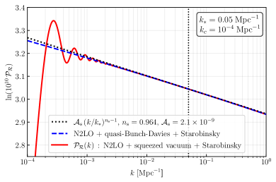
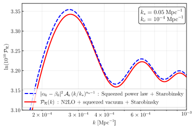
Figure 1: (Left): As an illustrative example, we compare the squeezed power spectrum $\mathcal{P}_{\mathrm{sqz}}(k)$ (solid red line) corresponding to the Bogoliubov coefficients (38) and (39), with the an exact power law (dotted black) and the N2LO expression for the qBD state (dashed blue). The values of the Hubble-flow parameters are the ones predicted by Starobinsky inflation with fiducial $N_{\ast}=55$, as discussed in [78] given in Tab. 1. The vertical black dotted line corresponds to the pivot scale $k_{\ast}$ typically used in CMB observations. (Right): We compare the squeezed power $\mathcal{P}_{\mathrm{sqz}}(k)$ with the standard expression associated to the same power law as in the left panel, i.e., setting artificially $\delta_{k}=0$ to show its effect of the power spectrum.

Figure 2: To further illustrate the effect of the phase $\delta_{k}$ we compare the N2LO result (V) (solid red) with the expression with $\delta_{k}=0$ artificially set to zero (dashed blue), adopting exaggerated values of the Hubble-flow parameters $\epsilon_{2H\ast}=-0.2$, $\epsilon_{2Z\ast}=-0.2$, to show a noticeable running. We compare them to the power spectrum produced by an exact power law (dotted black), with the same Bogoliubov coefficients (38)–(39). The other Hubble-flow parameters and pivot scales are taken from Tab. 1.

To illustrate the effect of the non-trivial phase $\delta_{k}$ on the squeezed power spectrum (28), we consider a simple choice of squeezed vacuum $|\mathrm{sqz}\rangle$ given by the Bogoliubov coefficients

$$\alpha_{k} =1-\frac{k_{c}^{2}}{2k^{2}}-\mathrm{i}\,\frac{k_{c}}{k}\,,$$ (38)

$$\beta_{k} =-\frac{k_{c}^{2}}{2k^{2}}\,\,\mathrm{e}^{\,2\,\mathrm{i}k/k_{c}}.$$ (39)

This specific choice has been considered and studied before (see for instance [43, 49, 53] and the review [20]) and can be understood as a simplified model of the effect of a pre-inflationary phase. In this model, one considers an instantaneous transition from Minkowski space to de Sitter space, i.e., a scale factor $a(t)$ given by

$$a(t)=\begin{cases}\frac{k_{c}}{H_{0}}\qquad&t<0\,,\\[5.0pt] \frac{k_{c}}{H_{0}}\,\mathrm{e}^{H_{0}t}\qquad\quad&t\geq 0\,,\end{cases}$$ (40)

where $k_{c}$ is a new physical scale defined as the comoving scale at the transition time $t=0$. In this situation there are two natural choices of state, the in-vacuum given by the Minkowski state $|\mathrm{M}\rangle$ for $t<0$ and the out-vacuum given by the Bunch-Davies state $|\mathrm{BD}\rangle$ for $t\geq 0$. They correspond to the mode functions $w_{M}(y)=\mathrm{e}^{\mathrm{i}y}$ for $y<y_{c}$ and $w_{\mathrm{BD}}(y)$ for $y\geq y_{c}$, (17), with $y_{c}\equiv k/k_{c}$. If a quantum field is prepared in the in-vacuum, the mode functions after the transition can be written as $w_{\mathrm{sqz}}(y)=\alpha_{k}\,w_{\mathrm{BD}}(y)+\beta_{k}\,w_{\mathrm{BD}}^{*}(y)$ with the Bogoliubov coefficients (38)–(39) determined by the matching of the mode function and its derivative at the time $y=y_{c}$, i.e., $w_{\mathrm{sqz}}(y_{c})=w_{\mathrm{M}}(y_{c})$ and $w_{\mathrm{sqz}}^{\prime}(y_{c})=w_{\mathrm{M}}^{\prime}(y_{c})$. While the model is not realistic, it provides a well-defined fiducial prescription for the Bogoliubov coefficients in terms of one single new physical scale, the comoving scale $k_{c}$ at the transition, and allows us to illustrate the effect of the phase shift $\delta_{k}$ determined in (36).

Table 1: Numerical values of Hubble-flow parameters and pivot scales to be used in the numerical analysis.

Parameters	Starobinsky values
$\epsilon_{1H\ast}$, $\epsilon_{2H\ast}$	$0.009,\,-0.018$
$\epsilon_{1Z\ast}$, $\epsilon_{2Z\ast}$	$-0.018,\,-0.018$
$\epsilon_{1c\ast}$ , $\epsilon_{2c\ast}$	$0,\,0$
$k_{\ast}=a_{\ast}H_{\ast}$	$5\times 10^{-2}$ Mpc-1
$k_{c}$	$2\times 10^{-4}$ Mpc-1

Assuming the squeezed state $|\mathrm{sqz}\rangle$ is defined exactly by the Bogoliubov coefficients (38)–(39), one finds that the squeezing factor (33), for $k\gg k_{c}$, takes the form

$$\Upsilon_{\mathrm{sqz}}(k)\, =1-2r_{k}\cos(\phi_{k}+\delta_{k})+\order{r_{k}^{2}}$$ (41)

$$=1-\frac{k_{c}^{2}}{k^{2}}\cos\Big(\frac{2k}{k_{c}}+\delta_{k}\Big{missing})+\order{k_{c}^{3}/k^{3}}\,.$$ (42)

This expression reproduces the form of the phenomenological template (1) with the phase shift $\delta_{k}$ now completely fixed by the background geometry, as determined in (36). As a concrete example for illustration, we consider the primordial power spectrum of scalar perturbations $\mathcal{R}(k)$ in the Starobinsky model of inflation [2, 3]. As discussed in [78], we can express all power-law quantities in the qBD vacuum up to N2LO in terms of a single parameter, the scalar tilt $n_{\mathrm{s}}$ which is also one of the most accurately measured cosmological parameters, $n_{\mathrm{s}}-1=-0.0351\pm 0.0042$ at $68\%$ CL [13]. Introducing an N2LO truncation in the parameter $|n_{\mathrm{s}}-1|\ll 1$, we find that the phase shift $\delta_{k}$ can be written as

$$\delta_{k}=\frac{\pi}{2}(n_{\mathrm{s}}-1)\,-\frac{\pi}{4}(n_{\mathrm{s}}-1)^{2}\,\ln\left(\frac{k}{k_{\ast}}\right)\,.$$ (43)

In particular we observe that, besides a constant negative phase shift proportional to $n_{\mathrm{s}}-1$, the phase $\delta_{k}$ introduces a running drift $\ln(k/k_{\ast})$ analogous to the one considered in phenomenological templates [25].

To illustrate concretely the features of the squeezed power spectrum described above, we consider Starobinsky inflation in the geometric framework, as discussed in [78]. We adopt fiducial values for the Hubble-flow parameters, which are the approximate figures at $N_{\ast}=55$ reported in Tab. 1. The new physical scale $k_{c}$ that characterizes the squeezed state $|\mathrm{sqz}\rangle$ via (38)–(39) is assumed here to take the fiducial value $k_{c}=10^{-4}$ Mpc^-1 corresponding to just-enough inflation [58, 59, 60, 61], that is a finite duration of the inflationary phase $N_{\mathrm{infl}}\sim 60$ that is not ruled out yet by observations and leads to features in the observable window of the power spectrum.

Fig. 1 illustrates the effect of phase $\delta_{k}$ at N2LO. The left panel in 1 shows a comparison between the exact power law used in phenomenological templates, the N2LO formula for the qBD vacuum derived in (III), and the squeezed power spectrum derived in this work up to N2LO, $\mathcal{P}_{\mathrm{sqz}}^{(\mathrm{N2LO})}(k)$ in equation (V). The squeezed vacuum corresponding to the specific choice of Bogoliubov coefficients (38) and (39), shows clear primordial features: a power suppression below to the physical scale $k_{c}$ and fast oscillations around $k_{c}$, rapidly converging to the tilted power associated to the quasi-Bunch-Davies vacuum at higher $k\gg k_{c}$. In the right panel of Fig. 1, we compare the effect of setting $\delta_{k}=0$ (as often done implicitly in previous works) with the full N2LO squeezed power $\mathcal{P}_{\mathrm{sqz}}^{(\mathrm{N2LO})}(k)$. Since Starobinsky inflation predicts small values of the Hubble-flow parameters, the difference is small, but still noticeable. To illustrate clearly the effect, in Fig. 2 we adopt an artificially enhanced set of Hubble-flow parameters, $\epsilon_{2H\ast}$ and $\epsilon_{2Z\ast}$. The larger values of these parameters induce a running of the tilt, which clearly deviates from the usual power-law expression. This scenario highlights the importance of extend the Hubble-flow analysis up to N2LO, as it allows to explore a combination of primordial features, i.e., from the squeezing factor and from deviations from de Sitter space.

VII Discussion

In this work we derived the effect of a squeezed vacuum on the primordial power spectrum. In particular we determined the phase $\delta_{k}$ appearing in (2) and computed its fully-expanded expression (36) around a pivot mode $k_{\ast}$, together with the power spectrum (V), for scalar and tensor perturbations in a large class of effective theories of inflation (3) characterized by a kinetic amplitude $Z_{\psi}(t)$ and speed of sound $c_{\psi}(t)$. In the case of Starobinsky inflation we found that the phase $\delta_{k}$ for curvature perturbations can be written purely in terms of the scalar tilt $n_{\mathrm{s}}$, resulting in a small negative shift together with a running drift (43), providing precision theoretical predictions that can be used in phenomenological templates for primordial features (1). It would be interesting to extend the analysis to other observables, including the bispectrum [20], and combine it with top-down proposals of new physics in a pre-inflationary phase [36, 37, 38, 39, 40, 41, 42, 43, 44, 45, 46, 47, 48, 49, 50, 51, 52, 53, 54, 55, 56, 57, 58, 59, 60, 61, 62, 63, 64, 65, 66, 67, 68, 69, 70, 71, 72, 73] to constrain the effect of primordial squeezed vacua with cosmological observations.

Appendix A Derivation of mode equation

Here we summarize some of the steps in the derivation of the mode equation, following [78]. First, note that for the original mode $u(k,t)$ satisfies the following canonical commutation relation (CCR),

$$u(k,t)\dot{u}^{\ast}(k,t)-\dot{u}(k,t)u^{\ast}(k,t)=\frac{\mathrm{i}\,\hbar}{2\,a(t)^{3}\,Z_{\psi}(t)},$$ (44)

where $u^{\ast}$ is the complex conjugate of $u$. On the other hand, the equation of motion (EoM) results in the mode equation

$$\ddot{u}(k,t)+(3-\epsilon_{Z1}(t))H(t)\dot{u}(k,t)+c_{\psi}(t)^{2}\frac{k^{2}}{a(t)^{2}}\,u(k,t)=0\,.$$ (45)

Under the map (11), the EoM becomes

$$w^{\prime\prime}(y)+\left[1+\frac{a(t)^{2}H(t)^{2}}{k\,c_{\psi}^{2}(t)}q(t)\right]w(y)=0,$$ (46)

where

$$q(t) =-2+\epsilon_{H1}(t)+\frac{3}{2}\epsilon_{Z1}(t)+\frac{\epsilon_{1c}(t)}{2}$$

$$\quad-\frac{\epsilon_{1H}(t)\epsilon_{1Z}(t)}{2}-\frac{\epsilon_{1Z}(t)^{2}}{4}-\frac{\epsilon_{1Z}(t)\epsilon_{2Z}(t)}{2}$$

$$\quad-\frac{\epsilon_{1c}(t)\epsilon_{1H}(t)}{2}-\frac{\epsilon_{1c}(t)\epsilon_{2c}(t)}{2}+\frac{\epsilon_{1c}^{2}(t)}{4}.$$ (47)

The above expression is exact in $\epsilon_{1H}(t)$, $\epsilon_{1Z}(t)$, $\epsilon_{1c}(t)$, etc. We then need to write $t$ (or, equivalently, a generalized conformal time $\tau$) as a function of $y$. This can be done self-consistently, as discussed in the Appendix A of [78], where we found that $\tau$ is, at N2LO, the following expression

$$\tau(t) =-\frac{c_{\psi}(t)}{a(t)H(t)}\Big{[}1+\epsilon_{1H}(t)-\epsilon_{1c}(t)+\epsilon_{1H}(t)^{2}-\epsilon_{1H}(t)\epsilon_{2H}(t)-2\epsilon_{1c}(t)\epsilon_{1H}(t)+\epsilon_{1c}(t)\epsilon_{2c}(t)+\epsilon_{1c}(t)^{2}+\mathcal{O}(\epsilon^{3})\Big{]}$$

$$\equiv-\frac{\,\tilde{c}_{\psi}(t)}{a(t)H(t)}\,.$$ (48)

Then, we define the variable $y\equiv-k\tau$, so we can use the above equation anytime we need $a(t)$ in terms of $y$. The next step is to write each flow parameter in terms of $y$, which can be done via the logarithmic expansion around the peculiar time $\tau_{k}\equiv-1/k$, i.e., around $y_{k}=1$.

$$\rho(y) =\rho_{k}\Big{[}1+\Big{(}\epsilon_{1\rho k}+\epsilon_{1\rho k}(\epsilon_{1Hk}-\epsilon_{1ck})\Big{)}\ln\left(y\right)+\frac{1}{2}\,\Big{(}\epsilon_{1\rho k}(\epsilon_{1\rho k}+\epsilon_{2\rho k})\Big{)}\ln\left(y\right)^{2}+\order{\epsilon^{3}}\Big{]}\,.$$ (49)

After replacing this expansion and introducing the variable $y$ into (14), we obtain the mode equation. Finally, by expanding $\mu(y)$ in the same way and replacing the limits (19), (20) and (21) into the expression for the power spectrum, we find the finite expression,

$$\mathcal{P}_{\mathrm{qBD}}^{(\mathrm{N2LO})}\;=\;\frac{\hbar\,H_{k}^{2}}{4\pi^{2}Z_{k}c_{k}^{3}}\Bigg{[}1+\Big{(}(2+3C)\,\epsilon_{1ck}-2(1+C)\,\epsilon_{1Hk}+C\,\epsilon_{1Zk}\Big{)}+\qquad$$

$$\quad+\frac{1}{24}\bigg{(}3(-64+24C+36C^{2}+9\pi^{2})\,\epsilon_{1ck}^{2}+12(-6+4C+4C^{2}+\pi^{2})\,\epsilon_{1Hk}^{2}$$

$$\qquad-3\,\epsilon_{1ck}\,\Big{(}4(-20+10C+12C^{2}+3\pi^{2})\,\epsilon_{1Hk}-2(-24+4C+12C^{2}+3\pi^{2})\,\epsilon_{1Zk}+(16+16C+12C^{2}-\pi^{2})\,\epsilon_{2ck}\Big{)}$$

$$\qquad-2\,\epsilon_{1Hk}\,\Big{(}6(-8+2C+4C^{2}+\pi^{2})\,\epsilon_{1Zk}+(-24-24C-12C^{2}+\pi^{2})\,\epsilon_{2Hk}\Big{)}$$

$$\qquad+\epsilon_{1Zk}\,\Big{(}3(-8+4C^{2}+\pi^{2})\,\epsilon_{1Zk}+(-12C^{2}+\pi^{2})\,\epsilon_{2Zk}\Big{)}\bigg{)}\;+\;\order{\epsilon^{3}}\Bigg{]}\,,$$ (50)

Later in the calculation, we need to expand the variables around a different time, characterized by a time $\tau_{\ast}=-1/k_{\ast}$, characterized by the pivot scale $k_{\ast}=a_{\ast}H_{\ast}/\tilde{c}_{\ast}$ This is an expansion around $y_{\ast}=k/k_{\ast}$,

$$\rho(y) =\rho_{\ast}\Big{[}1+\Big{(}\epsilon_{1\rho\ast}+\epsilon_{1\rho\ast}(\epsilon_{1H\ast}-\epsilon_{1c\ast})\Big{)}\ln\left(\frac{y}{y_{\ast}}\right)+\frac{1}{2}\,\Big{(}\epsilon_{1\rho\ast}(\epsilon_{1\rho\ast}+\epsilon_{2\rho\ast})\Big{)}\ln\left(\frac{y}{y_{\ast}}\right)^{2}+\order{\epsilon^{3}}\Big{]}\,.$$ (51)

Evaluating the above expression at $y_{k}$, gives the translation between quantities evaluated at the peculiar time $\tau_{k}=-1/k$ and the pivot time $\tau_{\ast}=-1/k_{\ast}$. Since $\ln(y/y_{\ast})=-\ln(k/k_{\ast})$, the expansion reads,

$$\rho_{k}=\rho(y_{k})=\rho_{\ast}\Big{[}1-\Big{(}\epsilon_{1\rho\ast}+\epsilon_{1\rho\ast}(\epsilon_{1H\ast}-\epsilon_{1c\ast})\Big{)}\ln\left(\frac{k}{k_{\ast}}\right)+\frac{1}{2}\,\Big{(}\epsilon_{1\rho\ast}(\epsilon_{1\rho\ast}+\epsilon_{2\rho\ast})\Big{)}\ln\left(\frac{k}{k_{\ast}}\right)^{2}+\order{\epsilon^{3}}\Big{]}\,.$$ (52)

The above evaluation introduces the logarithmic dependance of the power spectrum. Direct computation of all the quantities gives the following result,

$$\mathcal{P}_{\mathrm{qBD}}^{(\mathrm{N2LO})}(k) =\frac{\hbar\,H_{\ast}^{2}}{4\pi^{2}Z_{\ast}c_{\ast}^{3}}\Bigg{[}p_{0\ast}+p_{1\ast}\ln(\frac{k}{k_{\ast}})+p_{2\ast}\ln(\frac{k}{k_{\ast}})^{2}\Bigg{]}$$ (53)

with the coefficients,

$$p_{0\ast} =1\,-2(1+C)\epsilon_{1H\ast}+C\epsilon_{1Z\ast}+(2+3C)\epsilon_{1c\ast}$$

$$\quad+\frac{1}{24}\Bigg{(}3(-64+24C+36C^{2}+9\pi^{2})\epsilon_{1c\ast}^{2}+12(-6+4C+4C^{2}+\pi^{2})\epsilon_{1H\ast}^{2}$$

$$\quad-3\epsilon_{1c\ast}\Big{(}4(-20+10C+12C^{2}+3\pi^{2})\epsilon_{1H\ast}-2(-24+4C+12C^{2}+3\pi^{2})\epsilon_{1Z\ast}+(16+16C+12C^{2}-\pi^{2})\epsilon_{2c\ast}\Big{)}$$

$$\quad-2\epsilon_{1H\ast}\Big{(}6(-8+2C+4C^{2}+\pi^{2})\epsilon_{1Z\ast}+(-24-24C-12C^{2}+\pi^{2})\epsilon_{2H\ast}\Big{)}$$

$$\quad+\epsilon_{1Z\ast}\Big{(}3(-8+4C^{2}+\pi^{2})\epsilon_{1Z\ast}+(-12C^{2}+\pi^{2})\epsilon_{2Z\ast}\Big{)}\Bigg{)}$$ (54)

$$p_{1\ast} =3\epsilon_{1c\ast}-2\epsilon_{1H\ast}+\epsilon_{1Z\ast}$$

$$\quad+\Bigg{(}(3+9C)\epsilon_{1c\ast}^{2}+(2+4C)\epsilon_{1H\ast}^{2}+\epsilon_{1c\ast}\left(-(5+12C)\epsilon_{1H\ast}+\epsilon_{1Z\ast}+6C\epsilon_{1Z\ast}-2\epsilon_{2c\ast}-3C\epsilon_{2c\ast}\right)$$

$$\quad-\epsilon_{1H\ast}\left(\epsilon_{1Z\ast}+4C\epsilon_{1Z\ast}-2(1+C)\epsilon_{2H\ast}\right)+C\epsilon_{1Z\ast}\left(\epsilon_{1Z\ast}-\epsilon_{2Z\ast}\right)\Bigg{)}$$ (55)

$$p_{2\ast} =\frac{1}{2}\Bigg{(}9\epsilon_{1c\ast}^{2}+4\epsilon_{1H\ast}^{2}-4\epsilon_{1H\ast}\epsilon_{1Z\ast}+\epsilon_{1Z\ast}^{2}-3\epsilon_{1c\ast}\left(4\epsilon_{1H\ast}-2\epsilon_{1Z\ast}+\epsilon_{2c\ast}\right)+2\epsilon_{1H\ast}\epsilon_{2H\ast}-\epsilon_{1Z\ast}\epsilon_{2Z\ast}\Bigg{)}$$ (56)

References

- Brout et al. [1978] R. Brout, F. Englert, and E. Gunzig, The creation of the universe as a quantum phenomenon., Annals of Physics 115, 78 (1978).
- Starobinsky [1979] A. A. Starobinsky, Spectrum of relict gravitational radiation and the early state of the universe, JETP Lett. 30, 682 (1979).
- Starobinsky [1980] A. A. Starobinsky, A new type of isotropic cosmological models without singularity, Physics Letters B 91, 99 (1980).
- Guth [1981] A. H. Guth, Inflationary universe: A possible solution to the horizon and flatness problems, Phys. Rev. D 23, 347 (1981).
- Mukhanov and Chibisov [1981] V. F. Mukhanov and G. V. Chibisov, Quantum Fluctuations and a Nonsingular Universe, JETP Lett. 33, 532 (1981).
- Linde [1982] A. D. Linde, A new inflationary universe scenario: A possible solution of the horizon, flatness, homogeneity, isotropy and primordial monopole problems, Physics Letters B 108, 389 (1982).
- Albrecht and Steinhardt [1982] A. Albrecht and P. J. Steinhardt, Cosmology for Grand Unified Theories with Radiatively Induced Symmetry Breaking, Phys. Rev. Lett. 48, 1220 (1982).
- Guth and Pi [1982] A. H. Guth and S. Y. Pi, Fluctuations in the new inflationary universe, Phys. Rev. Lett. 49, 1110 (1982).
- Hawking [1982] S. W. Hawking, The development of irregularities in a single bubble inflationary universe, Phys. Lett. B 115, 295 (1982).
- Linde [1983] A. D. Linde, Chaotic inflation, Phys. Lett. B 129, 177 (1983).
- Mukhanov et al. [1992] V. F. Mukhanov, H. A. Feldman, and R. H. Brandenberger, Theory of cosmological perturbations, Phys. Rept. 215, 203 (1992).
- Martin et al. [2024] J. Martin, C. Ringeval, and V. Vennin, Cosmic Inflation at the Crossroads, (2024), arXiv:2404.10647 [astro-ph.CO] .
- Akrami et al. [2020] Y. Akrami et al. (Planck), Planck 2018 results. X. Constraints on inflation, Astron. Astrophys. 641, A10 (2020), arXiv:1807.06211 [astro-ph.CO] .
- CORE Collaboration et al. [2016] CORE Collaboration, F. Finelli, M. Bucher, A. Achúcarro, et al., Exploring cosmic origins with core: Inflation, Journal of Cosmology and Astroparticle Physics 2018 (04), 016, arXiv:1612.08270 [astro-ph.CO] .
- S4 Collaboration et al. [2020] S4 Collaboration, K. Abazajian, G. E. Addison, P. Adshead, et al., Cmb-s4: Forecasting constraints on primordial gravitational waves, The Astrophysical Journal 926, 54 (2020), arXiv:2008.12619 [astro-ph.CO] .
- LiteBIRD Collaboration [2022] LiteBIRD Collaboration, Probing cosmic inflation with the litebird cosmic microwave background polarization survey, Progress of Theoretical and Experimental Physics 2023, 10.1093/ptep/ptac150 (2022), arXiv:2202.02773 [astro-ph.IM] .
- Ballardini et al. [2024a] M. Ballardini et al. (Euclid), Euclid: The search for primordial features, Astron. Astrophys. 683, A220 (2024a), arXiv:2309.17287 [astro-ph.CO] .
- Mergulhão et al. [2023] T. Mergulhão, F. Beutler, and J. A. Peacock, Primordial feature constraints from BOSS + eBOSS, JCAP 08, 012, arXiv:2303.13946 [astro-ph.CO] .
- Antony et al. [2024] A. Antony, F. Finelli, D. K. Hazra, D. Paoletti, and A. Shafieloo, A search for super-imposed oscillations to the primordial power spectrum in Planck and SPT-3G 2018 data, (2024), arXiv:2403.19575 [astro-ph.CO] .
- Chluba et al. [2015] J. Chluba, J. Hamann, and S. P. Patil, Features and New Physical Scales in Primordial Observables: Theory and Observation, Int. J. Mod. Phys. D 24, 1530023 (2015), arXiv:1505.01834 [astro-ph.CO] .
- Achucarro et al. [2011] A. Achucarro, J.-O. Gong, S. Hardeman, G. A. Palma, and S. P. Patil, Features of heavy physics in the CMB power spectrum, JCAP 01, 030, arXiv:1010.3693 [hep-ph] .
- Hazra et al. [2010] D. K. Hazra, M. Aich, R. K. Jain, L. Sriramkumar, and T. Souradeep, Primordial features due to a step in the inflaton potential, JCAP 10, 008, arXiv:1005.2175 [astro-ph.CO] .
- Chen [2012] X. Chen, Primordial Features as Evidence for Inflation, JCAP 01, 038, arXiv:1104.1323 [hep-th] .
- Jackson and Shiu [2013] M. G. Jackson and G. Shiu, Study of the consistency relation for single-field inflation with power spectrum oscillations, Phys. Rev. D 88, 123511 (2013), arXiv:1303.4973 [hep-th] .
- Flauger et al. [2017] R. Flauger, L. McAllister, E. Silverstein, and A. Westphal, Drifting Oscillations in Axion Monodromy, JCAP 10, 055, arXiv:1412.1814 [hep-th] .
- Ballardini et al. [2016] M. Ballardini, F. Finelli, C. Fedeli, and L. Moscardini, Probing primordial features with future galaxy surveys, JCAP 10, 041, [Erratum: JCAP 04, E01 (2018)], arXiv:1606.03747 [astro-ph.CO] .
- Palma et al. [2018] G. A. Palma, D. Sapone, and S. Sypsas, Constraints on inflation with LSS surveys: features in the primordial power spectrum, JCAP 06, 004, arXiv:1710.02570 [astro-ph.CO] .
- L’Huillier et al. [2018] B. L’Huillier, A. Shafieloo, D. K. Hazra, G. F. Smoot, and A. A. Starobinsky, Probing features in the primordial perturbation spectrum with large-scale structure data, Mon. Not. Roy. Astron. Soc. 477, 2503 (2018), arXiv:1710.10987 [astro-ph.CO] .
- Zeng et al. [2019] C. Zeng, E. D. Kovetz, X. Chen, Y. Gong, J. B. Muñoz, and M. Kamionkowski, Searching for Oscillations in the Primordial Power Spectrum with CMB and LSS Data, Phys. Rev. D 99, 043517 (2019), arXiv:1812.05105 [astro-ph.CO] .
- Ballardini [2019] M. Ballardini, Probing primordial features with the primary CMB, Phys. Dark Univ. 23, 100245 (2019), arXiv:1807.05521 [astro-ph.CO] .
- Beutler et al. [2019] F. Beutler, M. Biagetti, D. Green, A. Slosar, and B. Wallisch, Primordial Features from Linear to Nonlinear Scales, Phys. Rev. Res. 1, 033209 (2019), arXiv:1906.08758 [astro-ph.CO] .
- Domènech and Kamionkowski [2019] G. Domènech and M. Kamionkowski, Lensing anomaly and oscillations in the primordial power spectrum, JCAP 11, 040, arXiv:1905.04323 [astro-ph.CO] .
- Slosar et al. [2019] A. Slosar et al., Scratches from the Past: Inflationary Archaeology through Features in the Power Spectrum of Primordial Fluctuations, Bull. Am. Astron. Soc. 51, 98 (2019), arXiv:1903.09883 [astro-ph.CO] .
- Braglia et al. [2021] M. Braglia, X. Chen, and D. K. Hazra, Probing Primordial Features with the Stochastic Gravitational Wave Background, JCAP 03, 005, arXiv:2012.05821 [astro-ph.CO] .
- Hamann and Wons [2022] J. Hamann and J. Wons, Optimising inflationary features the Bayesian way, JCAP 03 (03), 036, arXiv:2112.08571 [astro-ph.CO] .
- Vilenkin and Ford [1982] A. Vilenkin and L. H. Ford, Gravitational Effects upon Cosmological Phase Transitions, Phys. Rev. D 26, 1231 (1982).
- Starobinsky [1992] A. A. Starobinsky, Spectrum of adiabatic perturbations in the universe when there are singularities in the inflation potential, JETP Lett. 55, 489 (1992).
- Niemeyer [2001] J. C. Niemeyer, Inflation with a Planck scale frequency cutoff, Phys. Rev. D 63, 123502 (2001), arXiv:astro-ph/0005533 .
- Tanaka [2000] T. Tanaka, A Comment on transPlanckian physics in inflationary universe, (2000), arXiv:astro-ph/0012431 .
- Starobinsky [2001] A. A. Starobinsky, Robustness of the inflationary perturbation spectrum to transPlanckian physics, Pisma Zh. Eksp. Teor. Fiz. 73, 415 (2001), arXiv:astro-ph/0104043 .
- Hui and Kinney [2002] L. Hui and W. H. Kinney, Short distance physics and the consistency relation for scalar and tensor fluctuations in the inflationary universe, Phys. Rev. D 65, 103507 (2002), arXiv:astro-ph/0109107 .
- Goldstein and Lowe [2003] K. Goldstein and D. A. Lowe, Initial state effects on the cosmic microwave background and transPlanckian physics, Phys. Rev. D 67, 063502 (2003), arXiv:hep-th/0208167 .
- Danielsson [2002] U. H. Danielsson, A Note on inflation and transPlanckian physics, Phys. Rev. D 66, 023511 (2002), arXiv:hep-th/0203198 .
- Niemeyer et al. [2002] J. C. Niemeyer, R. Parentani, and D. Campo, Minimal modifications of the primordial power spectrum from an adiabatic short distance cutoff, Phys. Rev. D 66, 083510 (2002), arXiv:hep-th/0206149 .
- Contaldi et al. [2003] C. R. Contaldi, M. Peloso, L. Kofman, and A. D. Linde, Suppressing the lower multipoles in the CMB anisotropies, JCAP 07, 002, arXiv:astro-ph/0303636 .
- Martin and Brandenberger [2003] J. Martin and R. Brandenberger, On the dependence of the spectra of fluctuations in inflationary cosmology on transPlanckian physics, Phys. Rev. D 68, 063513 (2003), arXiv:hep-th/0305161 .
- Armendariz-Picon and Lim [2003] C. Armendariz-Picon and E. A. Lim, Vacuum choices and the predictions of inflation, JCAP 12, 006, arXiv:hep-th/0303103 .
- Bozza et al. [2003] V. Bozza, M. Giovannini, and G. Veneziano, Cosmological perturbations from a new physics hypersurface, JCAP 05, 001, arXiv:hep-th/0302184 .
- Danielsson [2005] U. H. Danielsson, Transplanckian energy production and slow roll inflation, Phys. Rev. D 71, 023516 (2005), arXiv:hep-th/0411172 .
- Wang and Ng [2008] I.-C. Wang and K.-W. Ng, Effects of a pre-inflation radiation-dominated epoch to CMB anisotropy, Phys. Rev. D 77, 083501 (2008), arXiv:0704.2095 [astro-ph] .
- Destri et al. [2010] C. Destri, H. J. de Vega, and N. G. Sanchez, The pre-inflationary and inflationary fast-roll eras and their signatures in the low CMB multipoles, Phys. Rev. D 81, 063520 (2010), arXiv:0912.2994 [astro-ph.CO] .
- Chen and Lin [2016] P. Chen and Y.-H. Lin, What initial condition of inflation would suppress the large-scale CMB spectrum?, Phys. Rev. D 93, 023503 (2016), arXiv:1505.05980 [gr-qc] .
- Broy [2016] B. J. Broy, Corrections to and from high scale physics, Phys. Rev. D 94, 103508 (2016), [Addendum: Phys.Rev.D 94, 109901 (2016)], arXiv:1609.03570 [hep-th] .
- Handley et al. [2016] W. J. Handley, A. N. Lasenby, and M. P. Hobson, Novel quantum initial conditions for inflation, Phys. Rev. D 94, 024041 (2016), arXiv:1607.04148 [gr-qc] .
- Kaloper and Scargill [2019] N. Kaloper and J. Scargill, Quantum Cosmic No-Hair Theorem and Inflation, Phys. Rev. D 99, 103514 (2019), arXiv:1802.09554 [hep-th] .
- Gessey-Jones and Handley [2021] T. Gessey-Jones and W. J. Handley, Constraining quantum initial conditions before inflation, Phys. Rev. D 104, 063532 (2021), arXiv:2104.03016 [astro-ph.CO] .
- Letey et al. [2024] M. I. Letey, Z. Shumaylov, F. J. Agocs, W. J. Handley, M. P. Hobson, and A. N. Lasenby, Quantum initial conditions for curved inflating universes, Phys. Rev. D 109, 123502 (2024), arXiv:2211.17248 [gr-qc] .
- Schwarz and Ramirez [2009] D. J. Schwarz and E. Ramirez, Just enough inflation, in 12th Marcel Grossmann Meeting on General Relativity (2009) pp. 1241–1243, arXiv:0912.4348 [hep-ph] .
- Ramirez and Schwarz [2012] E. Ramirez and D. J. Schwarz, Predictions of just-enough inflation, Phys. Rev. D 85, 103516 (2012), arXiv:1111.7131 [astro-ph.CO] .
- Ramirez [2012] E. Ramirez, Low power on large scales in just enough inflation models, Phys. Rev. D 85, 103517 (2012), arXiv:1202.0698 [astro-ph.CO] .
- Cicoli et al. [2014] M. Cicoli, S. Downes, B. Dutta, F. G. Pedro, and A. Westphal, Just enough inflation: power spectrum modifications at large scales, JCAP 12, 030, arXiv:1407.1048 [hep-th] .
- Agullo et al. [2012] I. Agullo, A. Ashtekar, and W. Nelson, A Quantum Gravity Extension of the Inflationary Scenario, Phys. Rev. Lett. 109, 251301 (2012), arXiv:1209.1609 [gr-qc] .
- Fernandez-Mendez et al. [2012] M. Fernandez-Mendez, G. A. Mena Marugan, and J. Olmedo, Hybrid quantization of an inflationary universe, Phys. Rev. D 86, 024003 (2012), arXiv:1205.1917 [gr-qc] .
- Fernandez-Mendez et al. [2013] M. Fernandez-Mendez, G. A. Mena Marugan, and J. Olmedo, Hybrid quantization of an inflationary model: The flat case, Phys. Rev. D 88, 044013 (2013), arXiv:1307.5222 [gr-qc] .
- Agullo et al. [2013] I. Agullo, A. Ashtekar, and W. Nelson, The pre-inflationary dynamics of loop quantum cosmology: Confronting quantum gravity with observations, Class. Quant. Grav. 30, 085014 (2013), arXiv:1302.0254 [gr-qc] .
- Agullo and Morris [2015] I. Agullo and N. A. Morris, Detailed analysis of the predictions of loop quantum cosmology for the primordial power spectra, Phys. Rev. D 92, 124040 (2015), arXiv:1509.05693 [gr-qc] .
- de Blas and Olmedo [2016] D. M. de Blas and J. Olmedo, Primordial power spectra for scalar perturbations in loop quantum cosmology, JCAP 06, 029, arXiv:1601.01716 [gr-qc] .
- Castello Gomar et al. [2017] L. Castello Gomar, G. A. Mena Marugan, D. Martin De Blas, and J. Olmedo, Hybrid loop quantum cosmology and predictions for the cosmic microwave background, Phys. Rev. D 96, 103528 (2017), arXiv:1702.06036 [gr-qc] .
- Bhardwaj et al. [2019] A. Bhardwaj, E. J. Copeland, and J. Louko, Inflation in Loop Quantum Cosmology, Phys. Rev. D 99, 063520 (2019), arXiv:1812.06841 [gr-qc] .
- Ashtekar et al. [2020] A. Ashtekar, B. Gupt, D. Jeong, and V. Sreenath, Alleviating the Tension in the Cosmic Microwave Background using Planck-Scale Physics, Phys. Rev. Lett. 125, 051302 (2020), arXiv:2001.11689 [astro-ph.CO] .
- Navascues and Marugan [2021] B. E. Navascues and G. A. M. Marugan, Analytical investigation of pre-inflationary effects in the primordial power spectrum: from General Relativity to hybrid Loop Quantum Cosmology, JCAP 09, 030, arXiv:2104.15002 [gr-qc] .
- Kowalczyk and Mena Marugan [2024] M. Kowalczyk and G. A. Mena Marugan, Choice of vacuum state and the relation between the inflationary and Planck scales, (2024), arXiv:2409.15886 [gr-qc] .
- Mena Marugan et al. [2024] G. A. Mena Marugan, A. Vicente-Becerril, and J. Yebana Carrilero, Analytic and numerical study of scalar perturbations in loop quantum cosmology, Phys. Rev. D 110, 043508 (2024), arXiv:2404.04595 [gr-qc] .
- Birrell and Davies [1982] N. D. Birrell and P. C. W. Davies, Quantum Fields in Curved Space, Cambridge Monographs on Mathematical Physics (Cambridge University Press, Cambridge, UK, 1982).
- Bunch and Davies [1978] T. S. Bunch and P. C. W. Davies, Quantum Field Theory in de Sitter Space: Renormalization by Point Splitting, Proc. Roy. Soc. Lond. A 360, 117 (1978).
- Ashtekar and Bianchi [2021] A. Ashtekar and E. Bianchi, A short review of loop quantum gravity, Rep. Prog. Phys. 84, 042001 (2021) 84, 042001 (2021), arXiv:2104.04394 [gr-qc] .
- Agullo et al. [2023] I. Agullo, A. Wang, and E. Wilson-Ewing, Loop quantum cosmology: relation between theory and observations 10.1007/978-981-19-3079-9_103-1 (2023), arXiv:2301.10215 [gr-qc] .
- Bianchi and Gamonal [2024] E. Bianchi and M. Gamonal, Primordial power spectrum at N3LO in effective theories of inflation, (2024), arXiv:2405.03157 [gr-qc] .
- Stewart and Gong [2001] E. D. Stewart and J.-O. Gong, The density perturbation power spectrum to second-order corrections in the slow-roll expansion, Phys.Lett.B510:1-9,2001 510, 1 (2001), arXiv:astro-ph/0101225 [astro-ph] .
- Auclair and Ringeval [2022] P. Auclair and C. Ringeval, Slow-roll inflation at N3LO, Phys. Rev. D 106, 063512 (2022) 106, 063512 (2022), arXiv:2205.12608 [astro-ph.CO] .
- Ballardini et al. [2024b] M. Ballardini, A. Davoli, and S. S. Sirletti, Third-order corrections to the slow-roll expansion: calculation and constraints with Planck, ACT, SPT, and BICEP/Keck, (2024b), arXiv:2408.05210 [astro-ph.CO] .
- Schwarz et al. [2001] D. J. Schwarz, C. A. Terrero-Escalante, and A. A. Garcia, Higher order corrections to primordial spectra from cosmological inflation, Phys. Lett. B 517, 243 (2001), arXiv:astro-ph/0106020 .